1 Introduction
In many applications it is important to control the dynamics of a fluid interface. A promising way to affect the fluid interface is the application of controlled vibrations. The present paper deals with the phenomenon observed in a two-layer system of immiscible viscous fluids subjected to horizontal vibrations: the Kelvin–Helmholtz instability in oscillatory flows.
In the experiments performed by Wolf (Reference Wolf1969) it was found that under sufficiently intensive horizontal vibrations, the interface between two layers of immiscible fluids becomes unstable, which results in the formation of a quasi-steady relief also called a ‘frozen wave’. This effect was confirmed experimentally by Bezdenezhnykh et al. (Reference Bezdenezhnykh, Briskman, Lapin, Lyubimov, Lyubimova, Tcherepanov and Zakharov1991, Reference Bezdenezhnykh, Briskman, Lyubimov, Lyubimova, Zakharov and Tcherepanov1992). Similar effects were observed in the experimental work of Shyh & Munson (Reference Shyh and Munson1986), where the angular vibrations were used instead of the linear vibrations. In all of the above studies, the frozen wave developed when the vibration intensity exceeded a specific threshold.
A theoretical explanation of the phenomenon was suggested by Lyubimov & Cherepanov (Reference Lyubimov and Cherepanov1987). Considering the case of small-amplitude high-frequency vibrations they showed that the frozen wave arises due to the development of the Kelvin–Helmholtz instability and derived the analytical expression for the critical vibration intensity. The instability was shown to be longwave in the case where the layer thickness is less than the critical value. For thicker layers the finite-wavelength instability is more dangerous, which leads to the formation of the frozen wave. The assumption of high-frequency vibrations was relaxed by Khenner et al. (Reference Khenner, Lyubimov, Belozerova and Roux1999). The calculations carried out for the case when the kinematic viscosities of the fluids are finite and equal showed that the Kelvin–Helmholtz instability is only slightly affected by viscosity. They also extended the Lyubimov & Cherepanov (Reference Lyubimov and Cherepanov1987) criterion of longwave instability dominance to the case of arbitrary vibration amplitude. The results of further studies including the consideration of fluid layers of different thicknesses can be found in the book by Lyubimov, Lyubimova & Cherepanov (Reference Lyubimov, Lyubimova and Cherepanov2003).
In addition to the Kelvin–Helmholtz instability mode, there are parametric instability modes found by Kelly (Reference Kelly1965). The quantitative inviscid theory for these modes was developed in (Lyubimov, Khenner & Shotz Reference Lyubimov, Khenner and Shotz1998), where the authors managed to reduce the problem to the solution of the Mathieu equation. As was shown in (Khenner et al. Reference Khenner, Lyubimov, Belozerova and Roux1999), this parametric instability is strongly damped by viscosity and in the majority of cases the Kelvin–Helmholtz mode is the most dangerous.
Lyubimov & Lyubimova (Reference Lyubimov and Lyubimova1990) developed a new method for numerical simulation of deformable interfaces, in which a volumetric force was introduced to model the effect of capillarity, and obtained governing equations for fluids of non-uniform density under high-frequency small-amplitude vibrations using the averaging method. These equations were used by the authors to investigate numerically the onset and nonlinear dynamics of the frozen wave. The critical parameters and the square root dependence of the frozen wave height on the supercriticality near the threshold agree well with the analytical solution of Lyubimov & Cherepanov (Reference Lyubimov and Cherepanov1987). In addition, it was found that the wavelength of the frozen wave grows with strengthening of vibrations and under vibrations of high intensity the system of two superposed horizontal layers is transformed into the system of nearly vertical bands.
Later on, the frozen wave formation was observed in a number of experimental works. In the experiments of Ivanova, Kozlov & Evesque (Reference Ivanova, Kozlov and Evesque2001a ) it was found that the wavelength of the frozen wave depends non-monotonically on the vibration frequency. The experimental study of supercritical regimes performed in Jalikop & Juel (Reference Jalikop and Juel2009) confirmed this result and showed that the height of the wave near the stability threshold grows as a square root of supercriticality, but then the dependence changes. The frozen wave was also observed in a two-phase system of liquid and vapour near the critical point by Wunenburger et al. (Reference Wunenburger, Evesque, Chabot, Garrabos, Fauve and Beysens1999) and Gandikota et al. (Reference Gandikota, Chatain, Amiroudine, Lyubimova and Beysens2014).
The results of experimental investigations of Bezdenezhnykh et al. (Reference Bezdenezhnykh, Briskman, Lapin, Lyubimov, Lyubimova, Tcherepanov and Zakharov1991, Reference Bezdenezhnykh, Briskman, Lyubimov, Lyubimova, Zakharov and Tcherepanov1992), Wunenburger et al. (Reference Wunenburger, Evesque, Chabot, Garrabos, Fauve and Beysens1999) and direct numerical simulations (DNS) of Lyubimov & Lyubimova (Reference Lyubimov and Lyubimova1990) are in good agreement with the inviscid theory developed by Lyubimov & Cherepanov (Reference Lyubimov and Cherepanov1987) for high frequencies. At the same time, the experiments for the systems of fluids with large viscosity contrast (where one of the fluids has a high enough viscosity) performed by Ivanova et al. (Reference Ivanova, Kozlov and Evesque2001a ), Ivanova, Kozlov & Tashkinov (Reference Ivanova, Kozlov and Tashkinov2001b ) demonstrated a significant deviation from the theoretical formula derived by Lyubimov & Cherepanov (Reference Lyubimov and Cherepanov1987) for the low and intermediate frequency range.
The effect of viscosity contrast on the linear stability threshold was studied in Talib, Jalikop & Juel (Reference Talib, Jalikop and Juel2007) and Talib & Juel (Reference Talib and Juel2007), where the problem was investigated experimentally and numerically using the spectral collocation method. The authors obtained neutral curves for finite amplitude and finite frequency vibrations. The analysis showed that in a wide range of viscosity ratios an increase in the viscosity contrast leads to destabilization, but in general the dependence of critical parameters on viscosity is non-monotonic. The condition for transition from the longwave to the finite-wavelength instability was found to be dependent on viscosity by demonstrating that the Khenner et al. (Reference Khenner, Lyubimov, Belozerova and Roux1999) criterion does not strictly hold for fluids with different viscosities.
Yoshikawa & Wesfreid (Reference Yoshikawa and Wesfreid2011) considered the viscosity effect on liquid layers of infinite depths. In this case, the perturbations with finite wavelength are more dangerous than the longwave ones (Lyubimov & Cherepanov Reference Lyubimov and Cherepanov1987) and the study focused on the development of the frozen wave. The results agree well with the results of the previous experimental works and linear stability analysis (Talib et al. Reference Talib, Jalikop and Juel2007; Talib & Juel Reference Talib and Juel2007; Jalikop & Juel Reference Jalikop and Juel2009). Note that in the above-mentioned papers, only a few situations are considered in which the longwave perturbations are the most dangerous.
In the present paper, we investigate the viscosity contrast effect on the longwave instability and the transition from the longwave to finite-wavelength instability. The paper is organized as follows. In § 2, the mathematical statement of the problem and the solution corresponding to a basic flow are given. In § 3, the problem of stability of the basic flow with respect to longwave perturbations is formulated and solved analytically. The obtained critical parameters are compared with the results obtained from the inviscid theory of Lyubimov & Cherepanov (Reference Lyubimov and Cherepanov1987) and the linear stability analysis of Talib & Juel (Reference Talib and Juel2007). In § 4, the boundary between the longwave and finite-wavelength instability domains in the parameter space is obtained. Our analytical results are verified by finding a numerical solution to the linear stability problem and by DNS. In § 5, all results are outlined and discussed.
2 Problem statement
2.1 Governing equations
A system of two horizontal layers of viscous immiscible fluids with deformable interface in an infinitely long rectangular container is considered. The layers are of the same thickness
 $h/2$
. The container is subjected to horizontal vibrations according to the law
 $a\cos \unicode[STIX]{x1D714}t$
where
 $a$
and
 $\unicode[STIX]{x1D714}$
are the amplitude and angular frequency of vibrations, respectively. The vibrations are assumed to be non-acoustic, which means that the acoustic wavelength at the vibration frequency is much greater than the layer thickness. Thus, the fluids can be treated as incompressible.
Based on the experimental data of Bezdenezhnykh et al. (Reference Bezdenezhnykh, Briskman, Lapin, Lyubimov, Lyubimova, Tcherepanov and Zakharov1991, Reference Bezdenezhnykh, Briskman, Lyubimov, Lyubimova, Zakharov and Tcherepanov1992), Ivanova et al. (Reference Ivanova, Kozlov and Evesque2001a
), Talib et al. (Reference Talib, Jalikop and Juel2007) and Jalikop & Juel (Reference Jalikop and Juel2009) we restrict ourselves to consideration of two-dimensional dynamics. We choose a Cartesian coordinate system in such a way that the
 $z$
-axis is directed vertically upwards, the
 $x$
-axis is horizontal and
 $z=0$
corresponds to the unperturbed interface, while the location of the deformed interface is determined by the equation
 $z=\unicode[STIX]{x1D709}(x,t)$
.
In the reference frame of the oscillating container, the system is governed by the continuity equation and by the Navier–Stokes equations, in which an additional term is introduced to describe the inertia force
 $$\begin{eqnarray}\frac{\unicode[STIX]{x2202}\boldsymbol{V}_{j}}{\unicode[STIX]{x2202}t}+\boldsymbol{V}_{j}\boldsymbol{\cdot }\unicode[STIX]{x1D735}\boldsymbol{V}_{j}=-\frac{1}{\unicode[STIX]{x1D70C}_{j}}\unicode[STIX]{x1D735}p+\unicode[STIX]{x1D708}_{j}\unicode[STIX]{x1D6FB}^{2}\boldsymbol{V}_{j}+\boldsymbol{g}+a\unicode[STIX]{x1D714}^{2}\boldsymbol{e}_{x}\cos \unicode[STIX]{x1D714}t.\end{eqnarray}$$
Here, the index
 $j$
denotes the fluid,
 $j=1$
corresponds to the upper fluid and
 $j=2$
to the lower fluid. On the rigid boundaries we impose the no-slip conditions
 $$\begin{eqnarray}\boldsymbol{V}|_{z=\pm h/2}=0.\end{eqnarray}$$
The boundary conditions imposed at the deformable interface are the normal and tangential stress balance, velocity continuity and kinematic condition, which are written as
 $$\begin{eqnarray}\displaystyle & \displaystyle \boldsymbol{n}\boldsymbol{\cdot }[\unicode[STIX]{x1D748}]_{\unicode[STIX]{x1D709}}\boldsymbol{\cdot }\boldsymbol{n}-[p]_{\unicode[STIX]{x1D709}}=\unicode[STIX]{x1D6FE}\unicode[STIX]{x1D735}\boldsymbol{\cdot }\boldsymbol{n}, & \displaystyle\end{eqnarray}$$
 $$\begin{eqnarray}\displaystyle & \displaystyle \boldsymbol{n}\boldsymbol{\cdot }[\unicode[STIX]{x1D748}]_{\unicode[STIX]{x1D709}}\boldsymbol{\cdot }\unicode[STIX]{x1D749}=0, & \displaystyle\end{eqnarray}$$
 $$\begin{eqnarray}\displaystyle & \displaystyle [\boldsymbol{V}]_{\unicode[STIX]{x1D709}}=0, & \displaystyle\end{eqnarray}$$
 $$\begin{eqnarray}\displaystyle & \displaystyle \frac{\unicode[STIX]{x2202}\unicode[STIX]{x1D709}}{\unicode[STIX]{x2202}t}=V_{z}|_{z=\unicode[STIX]{x1D709}(x,t)}-V_{x}|_{z=\unicode[STIX]{x1D709}(x,t)}\frac{\unicode[STIX]{x2202}\unicode[STIX]{x1D709}}{\unicode[STIX]{x2202}x}, & \displaystyle\end{eqnarray}$$
where the brackets denote a jump of the function across the interface,
 $$\begin{eqnarray}[F]_{\unicode[STIX]{x1D709}}=(F_{1}-F_{2})|_{z=\unicode[STIX]{x1D709}(x,t)},\end{eqnarray}$$
 $\unicode[STIX]{x1D6FE}$
is the surface tension coefficient,
 $\boldsymbol{n}$
and
 $\unicode[STIX]{x1D749}$
are the unit vectors normal and tangential to the interface, respectively, and
 $\unicode[STIX]{x1D748}$
is the viscous stress tensor.
To complete the mathematical formulation, an additional integral condition of flow closeness is imposed:
 $$\begin{eqnarray}\int _{-h/2}^{\unicode[STIX]{x1D709}}V_{x2}\,\text{d}z+\int _{\unicode[STIX]{x1D709}}^{h/2}V_{x1}\,\text{d}z=0.\end{eqnarray}$$
This constraint implies that the container is completely filled with fluids and there are no inlets or outlets.
The problem (2.1)–(2.8) is non-dimensionalized using
 $a\unicode[STIX]{x1D714},$
 $h$
,
 $h^{2}/(\unicode[STIX]{x1D708}_{1}+\unicode[STIX]{x1D708}_{2})$
,
 $\unicode[STIX]{x1D70C}_{1}+\unicode[STIX]{x1D70C}_{2}$
,
 $\unicode[STIX]{x1D708}_{1}+\unicode[STIX]{x1D708}_{2}$
and
 $a\unicode[STIX]{x1D714}(\unicode[STIX]{x1D70C}_{1}+\unicode[STIX]{x1D70C}_{2})(\unicode[STIX]{x1D708}_{1}+\unicode[STIX]{x1D708}_{2})$
as the scales of velocity, length, time, density, kinematic viscosity and pressure, respectively. With such scales, the dimensionless densities and viscosities are no longer the independent parameters and are determined by the corresponding ratios
 $\unicode[STIX]{x1D70C}_{r}=\unicode[STIX]{x1D70C}_{2}/\unicode[STIX]{x1D70C}_{1}$
and
 $\unicode[STIX]{x1D708}_{r}=\unicode[STIX]{x1D708}_{2}/\unicode[STIX]{x1D708}_{1}$
.
Then the Navier–Stokes equation (2.1) takes the following form:
 $$\begin{eqnarray}\frac{\unicode[STIX]{x2202}\boldsymbol{V}_{j}}{\unicode[STIX]{x2202}t}+Re\boldsymbol{V}_{j}\boldsymbol{\cdot }\unicode[STIX]{x1D735}\boldsymbol{V}_{j}=-\frac{1}{\unicode[STIX]{x1D70C}_{j}}\unicode[STIX]{x1D735}p+\unicode[STIX]{x1D708}_{j}\unicode[STIX]{x1D6FB}^{2}\boldsymbol{V}_{j}-\frac{Ga}{Re}\boldsymbol{e}_{z}+\unicode[STIX]{x1D6FA}\boldsymbol{e}_{x}\cos \unicode[STIX]{x1D6FA}t,\end{eqnarray}$$
and boundary conditions (2.3)–(2.6) at
 $z=\unicode[STIX]{x1D709}(x,t)$
are rewritten as
 $$\begin{eqnarray}\displaystyle & \displaystyle \frac{2}{Y}\left(\left[\unicode[STIX]{x1D70C}\unicode[STIX]{x1D708}\frac{\unicode[STIX]{x2202}V_{z}}{\unicode[STIX]{x2202}z}\right]_{\unicode[STIX]{x1D709}}-\frac{\unicode[STIX]{x2202}\unicode[STIX]{x1D709}}{\unicode[STIX]{x2202}x}\left[\unicode[STIX]{x1D70C}\unicode[STIX]{x1D708}\left(\frac{\unicode[STIX]{x2202}V_{x}}{\unicode[STIX]{x2202}z}+\frac{\unicode[STIX]{x2202}V_{z}}{\unicode[STIX]{x2202}x}\right)\right]_{\unicode[STIX]{x1D709}}+\left(\frac{\unicode[STIX]{x2202}\unicode[STIX]{x1D709}}{\unicode[STIX]{x2202}x}\right)^{2}\left[\unicode[STIX]{x1D70C}\unicode[STIX]{x1D708}\frac{\unicode[STIX]{x2202}V_{x}}{\unicode[STIX]{x2202}x}\right]_{\unicode[STIX]{x1D709}}\right)=S, & \displaystyle\end{eqnarray}$$
 $$\begin{eqnarray}\displaystyle & \displaystyle Y=1+\left(\frac{\unicode[STIX]{x2202}\unicode[STIX]{x1D709}}{\unicode[STIX]{x2202}x}\right)^{2}, & \displaystyle\end{eqnarray}$$
 $$\begin{eqnarray}\displaystyle & \displaystyle S=[p]_{\unicode[STIX]{x1D709}}+\frac{Ga[\unicode[STIX]{x1D70C}]}{ReBo}\frac{\unicode[STIX]{x2202}}{\unicode[STIX]{x2202}x}\left(Y^{-1/2}\frac{\unicode[STIX]{x2202}\unicode[STIX]{x1D709}}{\unicode[STIX]{x2202}x}\right), & \displaystyle\end{eqnarray}$$
 $$\begin{eqnarray}\displaystyle & \displaystyle (2-Y)\left[\unicode[STIX]{x1D70C}\unicode[STIX]{x1D708}\left(\frac{\unicode[STIX]{x2202}V_{x}}{\unicode[STIX]{x2202}z}+\frac{\unicode[STIX]{x2202}V_{z}}{\unicode[STIX]{x2202}x}\right)\right]_{\unicode[STIX]{x1D709}}+2\frac{\unicode[STIX]{x2202}\unicode[STIX]{x1D709}}{\unicode[STIX]{x2202}x}\left[\unicode[STIX]{x1D70C}\unicode[STIX]{x1D708}\left(\frac{\unicode[STIX]{x2202}V_{z}}{\unicode[STIX]{x2202}z}-\frac{\unicode[STIX]{x2202}V_{x}}{\unicode[STIX]{x2202}x}\right)\right]_{\unicode[STIX]{x1D709}}=0, & \displaystyle\end{eqnarray}$$
 $$\begin{eqnarray}\displaystyle & \displaystyle \frac{\unicode[STIX]{x2202}\unicode[STIX]{x1D709}}{\unicode[STIX]{x2202}t}=Re\left(V_{z}-V_{x}\frac{\unicode[STIX]{x2202}\unicode[STIX]{x1D709}}{\unicode[STIX]{x2202}x}\right)|_{z=\unicode[STIX]{x1D709}(x,t)}, & \displaystyle\end{eqnarray}$$
 $$\begin{eqnarray}\displaystyle & \displaystyle [\boldsymbol{V}]_{\unicode[STIX]{x1D709}}=0. & \displaystyle\end{eqnarray}$$
Here, the following parameters are introduced:
 $Re=a\unicode[STIX]{x1D714}h/(\unicode[STIX]{x1D708}_{1}+\unicode[STIX]{x1D708}_{2})$
is the Reynolds number,
 $\unicode[STIX]{x1D6FA}=\unicode[STIX]{x1D714}h^{2}/(\unicode[STIX]{x1D708}_{1}+\unicode[STIX]{x1D708}_{2})$
is the dimensionless frequency,
 $Ga=gh^{3}/(\unicode[STIX]{x1D708}_{1}+\unicode[STIX]{x1D708}_{2})^{2}$
is the Galileo number and
 $Bo=(\unicode[STIX]{x1D70C}_{2}-\unicode[STIX]{x1D70C}_{1})h^{2}g/\unicode[STIX]{x1D6FE}$
is the Bond number. It should be noted that the ratio
 $Re/\unicode[STIX]{x1D6FA}=a/h$
has the meaning of dimensionless amplitude of vibrations. For dimensionless variables the same notation is kept.
2.2 Basic flow
The system (2.9)–(2.15) has a solution, which corresponds to the undeformed interface,
 $\unicode[STIX]{x1D709}=0$
and one-dimensional pulsating flow, in which the vertical velocity component is zero, whereas the pressure and
 $x$
-component of velocity have the following form (Khenner et al.
Reference Khenner, Lyubimov, Belozerova and Roux1999):
 $$\begin{eqnarray}\displaystyle & \displaystyle p(x,z,t)=\unicode[STIX]{x1D6F1}_{[0]}(z)+\unicode[STIX]{x1D6F1}_{[+1]}(x)\exp (\text{i}\unicode[STIX]{x1D6FA}t)+\unicode[STIX]{x1D6F1}_{[-1]}(x)\exp (-\text{i}\unicode[STIX]{x1D6FA}t), & \displaystyle\end{eqnarray}$$
 $$\begin{eqnarray}\displaystyle & \displaystyle V_{x}(z,t)=U_{[+1]}(z)\exp (\text{i}\unicode[STIX]{x1D6FA}t)+U_{[-1]}(z)\exp (-\text{i}\unicode[STIX]{x1D6FA}t), & \displaystyle\end{eqnarray}$$
where
 $\unicode[STIX]{x1D6F1}_{[-1]}=\unicode[STIX]{x1D6F1}_{[+1]}^{\ast }$
and
 $U_{[-1]}=U_{[+1]}^{\ast }$
, and the asterisk denotes the complex conjugation.
Substituting this solution into the Navier–Stokes equations (2.9), we have
 $$\begin{eqnarray}\displaystyle & \displaystyle \mp \text{i}\unicode[STIX]{x1D70C}\unicode[STIX]{x1D6FA}U_{[\pm 1]}+\unicode[STIX]{x1D70C}\unicode[STIX]{x1D708}\frac{\text{d}^{2}}{\text{d}z^{2}}U_{[\pm 1]}=\frac{\unicode[STIX]{x2202}}{\unicode[STIX]{x2202}x}\unicode[STIX]{x1D6F1}_{[\pm 1]}-\frac{1}{2}\unicode[STIX]{x1D70C}\unicode[STIX]{x1D6FA}, & \displaystyle\end{eqnarray}$$
 $$\begin{eqnarray}\displaystyle & \displaystyle \frac{\unicode[STIX]{x2202}}{\unicode[STIX]{x2202}z}\unicode[STIX]{x1D6F1}_{[\pm 1]}=\frac{\unicode[STIX]{x2202}}{\unicode[STIX]{x2202}z}\unicode[STIX]{x1D6F1}_{[0]}+\unicode[STIX]{x1D70C}\frac{Ga}{Re}=0, & \displaystyle\end{eqnarray}$$
with the boundary conditions at the interface,
 $z=0$
:
 $$\begin{eqnarray}\displaystyle & \displaystyle [\unicode[STIX]{x1D6F1}_{[\pm 1]}]_{\unicode[STIX]{x1D709}}=[U_{[\pm 1]}]_{\unicode[STIX]{x1D709}}=0, & \displaystyle\end{eqnarray}$$
 $$\begin{eqnarray}\displaystyle & \displaystyle \left[\unicode[STIX]{x1D70C}\unicode[STIX]{x1D708}\frac{\unicode[STIX]{x2202}}{\unicode[STIX]{x2202}z}U_{[\pm 1]}\right]_{\unicode[STIX]{x1D709}}=0. & \displaystyle\end{eqnarray}$$
The solution of (2.18)–(2.19) has the following form (Talib & Juel Reference Talib and Juel2007):
 $$\begin{eqnarray}\displaystyle & \displaystyle U_{j[\pm 1]}=A_{j[\pm 1]}\exp \left((1\pm \text{i})\frac{z}{\unicode[STIX]{x1D6FF}_{j}}\right)+B_{j[\pm 1]}\exp \left(-(1\pm \text{i})\frac{z}{\unicode[STIX]{x1D6FF}_{j}}\right)+C_{j[\pm 1]}, & \displaystyle\end{eqnarray}$$
 $$\begin{eqnarray}\displaystyle & \displaystyle \unicode[STIX]{x1D6F1}_{[\pm 1]}=\unicode[STIX]{x1D70C}_{1}\left({\textstyle \frac{1}{2}}\mp \text{i}C_{1[\pm 1]}\right)\unicode[STIX]{x1D6FA}x=\unicode[STIX]{x1D70C}_{2}\left({\textstyle \frac{1}{2}}\mp \text{i}C_{2[\pm 1]}\right)\unicode[STIX]{x1D6FA}x\quad (j=1,2), & \displaystyle\end{eqnarray}$$
where
 $\unicode[STIX]{x1D6FF}_{j}=\sqrt{2\unicode[STIX]{x1D708}_{j}/\unicode[STIX]{x1D6FA}}$
is the dimensionless thickness of the Stokes boundary layer in the
 $j$
th fluid. Substituting this form of solution into boundary conditions (2.2), (2.8), (2.20) and (2.21), we obtain the linear system of algebraic equations for the constants
 $A_{j[\pm 1]}$
,
 $B_{j[\pm 1]}$
,
 $C_{j[\pm 1]}$
:
 $$\begin{eqnarray}\displaystyle & \displaystyle A_{1[\pm 1]}\exp \left(\frac{1\pm \text{i}}{2\unicode[STIX]{x1D6FF}_{1}}\right)+B_{1[\pm 1]}\exp \left(-\frac{1\pm \text{i}}{2\unicode[STIX]{x1D6FF}_{1}}\right)+C_{1[\pm 1]}=0, & \displaystyle\end{eqnarray}$$
 $$\begin{eqnarray}\displaystyle & \displaystyle A_{1[\pm 1]}+B_{1[\pm 1]}+C_{1[\pm 1]}=A_{2[\pm 1]}+B_{2[\pm 1]}+C_{2[\pm 1]}, & \displaystyle\end{eqnarray}$$
 $$\begin{eqnarray}\displaystyle & \displaystyle A_{2[\pm 1]}\exp \left(-\frac{1\pm \text{i}}{2\unicode[STIX]{x1D6FF}_{2}}\right)+B_{2[\pm 1]}\exp \left(\frac{1\pm \text{i}}{2\unicode[STIX]{x1D6FF}_{2}}\right)+C_{2[\pm 1]}=0, & \displaystyle\end{eqnarray}$$
 $$\begin{eqnarray}\displaystyle & \displaystyle \unicode[STIX]{x1D70C}_{1}\left({\textstyle \frac{1}{2}}\mp \text{i}C_{1[\pm 1]}\right)=\unicode[STIX]{x1D70C}_{2}\left({\textstyle \frac{1}{2}}\mp \text{i}C_{2[\pm 1]}\right), & \displaystyle\end{eqnarray}$$
 $$\begin{eqnarray}\displaystyle & \displaystyle \unicode[STIX]{x1D70C}_{1}\unicode[STIX]{x1D708}_{1}\frac{1\pm \text{i}}{\unicode[STIX]{x1D6FF}_{1}}(A_{1[\pm 1]}-B_{1[\pm 1]})=\unicode[STIX]{x1D70C}_{2}\unicode[STIX]{x1D708}_{2}\frac{1\pm \text{i}}{\unicode[STIX]{x1D6FF}_{2}}(A_{2[\pm 1]}-B_{2[\pm 1]}), & \displaystyle\end{eqnarray}$$
 $$\begin{eqnarray}\displaystyle & \displaystyle A_{1[\pm 11]}\frac{\unicode[STIX]{x1D6FF}_{1}}{1\pm \text{i}}\left\{\exp \left(\frac{1\pm \text{i}}{2\unicode[STIX]{x1D6FF}_{1}}\right)-1\right\}+B_{1[+1]}\frac{\unicode[STIX]{x1D6FF}_{1}}{1\pm \text{i}}\left\{\exp \left(-\frac{1\pm \text{i}}{2\unicode[STIX]{x1D6FF}_{1}}\right)-1\right\}+\frac{1}{2}C_{1[\pm 1]}\qquad & \displaystyle \nonumber\\ \displaystyle & \displaystyle \quad =A_{2[+1]}\frac{\unicode[STIX]{x1D6FF}_{2}}{1\pm \text{i}}\left\{1-\exp \left(-\frac{1\pm \text{i}}{2\unicode[STIX]{x1D6FF}_{2}}\right)\right\}+B_{2[\pm 1]}\frac{\unicode[STIX]{x1D6FF}_{2}}{1\pm \text{i}}\left\{1-\exp \left(\frac{1\pm \text{i}}{2\unicode[STIX]{x1D6FF}_{2}}\right)\right\}+\frac{1}{2}C_{2[\pm 1]}. & \displaystyle \nonumber\\ \displaystyle & & \displaystyle\end{eqnarray}$$
This system was solved using the Maple 10 package for symbolic calculations.
3 Linear stability threshold
Let us consider the stability of the interface against small perturbations. Since the problem is homogeneous with respect to the
 $x$
coordinate, we consider normal perturbations periodical in the
 $x$
direction. According to the Floquet method, the small normal perturbations of pressure
 $p$
, the
 $x$
-component of velocity
 $u$
, the
 $z$
-component of velocity
 $w$
and the interface position
 $\unicode[STIX]{x1D709}$
are searched for in the following form:
 $$\begin{eqnarray}\tilde{f}(x,z,t)=f(z,t)\exp (\unicode[STIX]{x1D706}t+\text{i}kx)+f^{\star }(z,t)\exp (\unicode[STIX]{x1D706}^{\star }t-\text{i}kx),\end{eqnarray}$$
where
 $f(z,t)=f(z,t+2\unicode[STIX]{x03C0}/\unicode[STIX]{x1D6FA})$
is the periodic function of time.
The linearized equations for small perturbations are written as
 $$\begin{eqnarray}\displaystyle & \displaystyle \unicode[STIX]{x1D706}u+\frac{\unicode[STIX]{x2202}u}{\unicode[STIX]{x2202}t}+\text{i}kReUu+Rew\frac{\unicode[STIX]{x2202}U}{\unicode[STIX]{x2202}z}=-\text{i}k\frac{p}{\unicode[STIX]{x1D70C}}+\unicode[STIX]{x1D708}\left(\frac{\unicode[STIX]{x2202}^{2}}{\unicode[STIX]{x2202}z^{2}}-k^{2}\right)u, & \displaystyle\end{eqnarray}$$
 $$\begin{eqnarray}\displaystyle & \displaystyle \unicode[STIX]{x1D706}w+\frac{\unicode[STIX]{x2202}w}{\unicode[STIX]{x2202}t}+\text{i}kReUw=-\frac{1}{\unicode[STIX]{x1D70C}}\frac{\unicode[STIX]{x2202}p}{\unicode[STIX]{x2202}z}+\unicode[STIX]{x1D708}\left(\frac{\unicode[STIX]{x2202}^{2}}{\unicode[STIX]{x2202}z^{2}}-k^{2}\right)w, & \displaystyle\end{eqnarray}$$
 $$\begin{eqnarray}\displaystyle & \displaystyle \frac{\unicode[STIX]{x2202}w}{\unicode[STIX]{x2202}z}+\text{i}ku=0. & \displaystyle\end{eqnarray}$$
In the linear stability analysis the interface deviations are assumed to be small, so that boundary conditions (2.12)–(2.15) can be shifted to the undisturbed position,
 $z=0$
. Keeping only
 $\unicode[STIX]{x1D709}$
-independent and linear with respect to
 $\unicode[STIX]{x1D709}$
terms, we obtain
 $$\begin{eqnarray}\displaystyle & \displaystyle 2\left[\unicode[STIX]{x1D70C}\unicode[STIX]{x1D708}\frac{\unicode[STIX]{x2202}w}{\unicode[STIX]{x2202}z}\right]-2\text{i}k\unicode[STIX]{x1D709}\left[\unicode[STIX]{x1D70C}\unicode[STIX]{x1D708}\frac{\unicode[STIX]{x2202}U}{\unicode[STIX]{x2202}z}\right]-[p]+\frac{Ga[\unicode[STIX]{x1D70C}]}{Re}\unicode[STIX]{x1D709}=k^{2}\frac{Ga[\unicode[STIX]{x1D70C}]}{ReBo}\unicode[STIX]{x1D709}, & \displaystyle\end{eqnarray}$$
 $$\begin{eqnarray}\displaystyle & \displaystyle \left[\unicode[STIX]{x1D70C}\unicode[STIX]{x1D708}\left(\frac{\unicode[STIX]{x2202}u}{\unicode[STIX]{x2202}z}+\text{i}kw\right)\right]+\unicode[STIX]{x1D709}\left[\unicode[STIX]{x1D70C}\unicode[STIX]{x1D708}\frac{\unicode[STIX]{x2202}^{2}U}{\unicode[STIX]{x2202}z^{2}}\right]=0, & \displaystyle\end{eqnarray}$$
 $$\begin{eqnarray}\displaystyle & \displaystyle [u]+\unicode[STIX]{x1D709}\left[\frac{\unicode[STIX]{x2202}U}{\unicode[STIX]{x2202}z}\right]=[w]=0, & \displaystyle\end{eqnarray}$$
 $$\begin{eqnarray}\displaystyle & \displaystyle \unicode[STIX]{x1D706}\unicode[STIX]{x1D709}+\frac{\unicode[STIX]{x2202}\unicode[STIX]{x1D709}}{\unicode[STIX]{x2202}t}=Re(w-\text{i}k\unicode[STIX]{x1D709}U)|_{z=0}, & \displaystyle\end{eqnarray}$$
with the no-slip conditions at the rigid walls:
 $$\begin{eqnarray}u|_{z=\pm 1/2}=w|_{z=\pm 1/2}=0.\end{eqnarray}$$
Hereinafter, the brackets denote a jump of the function across the interface
 $z=0$
:
 $[F]=(F_{1}-F_{2})|_{z=0}$
.
We consider the longwave perturbations, which allows us to perform a formal expansion of all fields in power series with respect to the small parameter
 $k$
:
 $$\begin{eqnarray}w=k\mathop{\sum }_{j=0}^{\infty }k^{j}w^{(j)},\quad \unicode[STIX]{x1D706}=\mathop{\sum }_{j=0}^{\infty }k^{j}\unicode[STIX]{x1D706}^{(j)},\end{eqnarray}$$
 $$\begin{eqnarray}p=k^{-1}\mathop{\sum }_{j=0}^{\infty }k^{j}p^{(j)},\quad u=\mathop{\sum }_{j=0}^{\infty }k^{j}u^{(j)},\end{eqnarray}$$
 $$\begin{eqnarray}\unicode[STIX]{x1D709}=\mathop{\sum }_{j=0}^{\infty }k^{j}\unicode[STIX]{x1D709}^{(j)}.\end{eqnarray}$$
A series expansion of pressure begins with
 $O(k^{-1})$
, since no solution can be found if
 $p$
and
 $u$
are the small quantities of the same order of magnitude.
According to the Floquet method, the fields
 $p$
,
 $u$
,
 $w$
and
 $\unicode[STIX]{x1D709}$
are the periodic functions of time, which in terms of the Fourier series can be written as
 $$\begin{eqnarray}f(z,t)=\mathop{\sum }_{n=-\infty }^{\infty }f_{[n]}(z)\exp (\text{i}n\unicode[STIX]{x1D6FA}t).\end{eqnarray}$$
In the leading (zeroth) order of series expansion, it follows from the kinematic condition (3.8) that
 $$\begin{eqnarray}\unicode[STIX]{x1D706}^{(0)}=0,\quad \text{for all }n\neq 0:\unicode[STIX]{x1D709}_{[n]}^{(0)}=0,\end{eqnarray}$$
 $$\begin{eqnarray}p_{[\pm 1]}^{(0)\prime }=0,\quad \unicode[STIX]{x1D708}u_{[\pm 1]}^{(0)\prime \prime }\pm \text{i}\unicode[STIX]{x1D6FA}u_{[\pm 1]}^{(0)}-\frac{\text{i}}{\unicode[STIX]{x1D70C}}p_{[\pm 1]}^{(0)}=0,\end{eqnarray}$$
 $$\begin{eqnarray}w_{[\pm 1]}^{(0)\prime }+\text{i}u_{[\pm 1]}^{(0)}=0,\end{eqnarray}$$
with the boundary conditions at
 $z=0$
:
 $$\begin{eqnarray}\displaystyle & \displaystyle [p_{[\pm 1]}^{(0)}]=0, & \displaystyle\end{eqnarray}$$
 $$\begin{eqnarray}\displaystyle & \displaystyle [\unicode[STIX]{x1D70C}\unicode[STIX]{x1D708}u_{[\pm 1]}^{(0)\prime }]=-\unicode[STIX]{x1D709}_{[0]}^{(0)}[\unicode[STIX]{x1D70C}\unicode[STIX]{x1D708}U_{[\pm 1]}^{\prime \prime }], & \displaystyle\end{eqnarray}$$
 $$\begin{eqnarray}\displaystyle & \displaystyle [u_{[\pm 1]}^{(0)}]=-\unicode[STIX]{x1D709}_{[0]}^{(0)}[U_{[\pm 1]}^{\prime }], & \displaystyle\end{eqnarray}$$
 $$\begin{eqnarray}\displaystyle & \displaystyle [w_{[\pm 1]}^{(0)}]=0, & \displaystyle\end{eqnarray}$$
and the no-slip conditions at the rigid walls
 $z=\pm 1/2$
:
 $$\begin{eqnarray}w_{[\pm 1]}^{(0)}=u_{[\pm 1]}^{(0)}=0.\end{eqnarray}$$
Hereinafter, the prime stands for a derivative with respect to the
 $z$
coordinate.
A solution is searched for in the following form:
 $$\begin{eqnarray}\displaystyle & \displaystyle u_{j[\pm 1]}^{(0)}=a_{j[\pm 1]}\exp \left((1\pm \text{i})\frac{z}{\unicode[STIX]{x1D6FF}_{j}}\right)+b_{j[\pm 1]}\exp \left(-(1\pm \text{i})\frac{z}{\unicode[STIX]{x1D6FF}_{j}}\right)\mp \frac{p_{[\pm 1]}^{(0)}}{\unicode[STIX]{x1D6FA}\unicode[STIX]{x1D70C}_{j}}, & \displaystyle\end{eqnarray}$$
 $$\begin{eqnarray}\displaystyle & \displaystyle w_{j[\pm 1]}^{(0)}=c_{j[\pm 1]}+\int u_{j[\pm 1]}^{(0)}\,\text{d}z. & \displaystyle\end{eqnarray}$$
Substituting (3.22)–(3.23) into (3.15)–(3.20) yields the coefficients
 $a_{j[\pm 1]}$
,
 $b_{j[\pm 1]}$
,
 $c_{j[\pm 1]}$
and
 $p_{[\pm 1]}^{(0)}$
with the only unknown
 $\unicode[STIX]{x1D709}_{[0]}^{(0)}$
, being a linear multiplication factor.
In the next order of series expansion, the kinematic condition (3.8) gives
 $$\begin{eqnarray}\unicode[STIX]{x1D706}^{(1)}=0,\quad \unicode[STIX]{x1D709}_{[\pm 1]}^{(1)}=\mp \text{i}\frac{Re}{\unicode[STIX]{x1D6FA}}(w_{[\pm 1]}^{(0)}-\text{i}\unicode[STIX]{x1D709}_{[0]}^{(0)}U_{[\pm 1]})|_{z=0},\end{eqnarray}$$
and the governing equations (3.2)–(3.4) are written as
 $$\begin{eqnarray}\displaystyle & \displaystyle p_{[0,\pm 2]}^{(1)\prime }=0, & \displaystyle\end{eqnarray}$$
 $$\begin{eqnarray}\displaystyle & \displaystyle u_{[0]}^{(1)\prime \prime }-\frac{\text{i}}{\unicode[STIX]{x1D70C}\unicode[STIX]{x1D708}}p_{[0]}^{(1)}=\frac{Re}{\unicode[STIX]{x1D708}}(\text{i}u_{[+1]}^{(0)}U_{[-1]}+\text{i}u_{[-1]}^{(0)}U_{[+1]}+w_{[+1]}^{(0)}U_{[-1]}^{\prime }+w_{[-1]}^{(0)}U_{[+1]}^{\prime }), & \displaystyle\end{eqnarray}$$
 $$\begin{eqnarray}\displaystyle & \displaystyle u_{[\pm 2]}^{(1)\prime \prime }-\frac{\text{i}}{\unicode[STIX]{x1D70C}\unicode[STIX]{x1D708}}p_{[\pm 2]}^{(1)}=\frac{Re}{\unicode[STIX]{x1D708}}(\text{i}u_{[\pm 1]}^{(0)}U_{[\pm 1]}+w_{[\pm 1]}^{(0)}U_{[\pm 1]}^{\prime }), & \displaystyle\end{eqnarray}$$
 $$\begin{eqnarray}\displaystyle & \displaystyle w_{[0,\pm 2]}^{(1)\prime }+\text{i}u_{[0,\pm 2]}^{(1)}=0, & \displaystyle\end{eqnarray}$$
with the boundary conditions at
 $z=0$
written as
 $$\begin{eqnarray}\displaystyle & \displaystyle [\unicode[STIX]{x1D70C}\unicode[STIX]{x1D708}u_{[0]}^{(1)\prime }]+\unicode[STIX]{x1D709}_{[+1]}^{(1)}[\unicode[STIX]{x1D70C}\unicode[STIX]{x1D708}U_{[-1]}^{\prime \prime }]+\unicode[STIX]{x1D709}_{[-1]}^{(1)}[\unicode[STIX]{x1D70C}\unicode[STIX]{x1D708}U_{[+1]}^{\prime \prime }]=[p_{[0]}^{(1)}]-[\unicode[STIX]{x1D70C}]\frac{Ga}{Re}\unicode[STIX]{x1D709}_{[0]}^{(0)}=0, & \displaystyle\end{eqnarray}$$
 $$\begin{eqnarray}\displaystyle & \displaystyle [u_{[0]}^{(1)}]+\unicode[STIX]{x1D709}_{[+1]}^{(1)}[U_{[-1]}^{\prime }]+\unicode[STIX]{x1D709}_{[-1]}^{(1)}[U_{[+1]}^{\prime }]=[w_{[0]}^{(1)}]=0, & \displaystyle\end{eqnarray}$$
 $$\begin{eqnarray}\displaystyle & \displaystyle [p_{[\pm 2]}^{(1)}]=[\unicode[STIX]{x1D70C}\unicode[STIX]{x1D708}u_{[\pm 2]}^{(1)\prime }]+\unicode[STIX]{x1D709}_{[\pm 1]}^{(0)}[\unicode[STIX]{x1D70C}\unicode[STIX]{x1D708}U_{[\pm 1]}^{\prime \prime }]=0, & \displaystyle\end{eqnarray}$$
 $$\begin{eqnarray}\displaystyle & \displaystyle [u_{[\pm 2]}^{(1)}]+\unicode[STIX]{x1D709}_{[\pm 1]}^{(1)}[U_{[\pm 1]}^{\prime }]=[w_{[\pm 2]}^{(1)}]=0, & \displaystyle\end{eqnarray}$$
and the no-slip conditions at the rigid walls.
The expressions for
 $p_{[0,\pm 2]}^{(1)}$
,
 $u_{[0,\pm 2]}^{(1)}$
and
 $w_{[0,\pm 2]}^{(1)}$
are found in terms of
 $\unicode[STIX]{x1D709}_{[0]}^{(0)}$
taken as a multiplication factor. However, they are too cumbersome to be presented here.
In the second order the following expressions are derived from the kinematic condition (3.8):
 $$\begin{eqnarray}\displaystyle & \displaystyle \unicode[STIX]{x1D706}^{(2)}\unicode[STIX]{x1D709}_{[0]}^{(0)}=\mp \text{i}Re(w_{[0]}^{(1)}-\text{i}(\unicode[STIX]{x1D709}_{[+1]}^{(1)}U_{[-1]}-\unicode[STIX]{x1D709}_{[-1]}^{(1)}U_{[+1]}))|_{z=0}, & \displaystyle\end{eqnarray}$$
 $$\begin{eqnarray}\displaystyle & \displaystyle \unicode[STIX]{x1D709}_{[\pm 2]}^{(2)}=\mp \text{i}\frac{Re}{2\unicode[STIX]{x1D6FA}}(w_{[\pm 2]}^{(1)}-\text{i}\unicode[STIX]{x1D709}_{[\pm 1]}^{(1)}U_{[\pm 1]})|_{z=0}. & \displaystyle\end{eqnarray}$$
The first of equations (3.33) determines
 $\unicode[STIX]{x1D706}^{(2)}$
as the function of
 $Re$
,
 $\unicode[STIX]{x1D6FA}$
,
 $Ga$
,
 $\unicode[STIX]{x1D70C}_{r}$
and
 $\unicode[STIX]{x1D708}_{r}$
. The calculations show that
 $\unicode[STIX]{x1D706}^{(2)}$
is a real value, which suggests that the instability is of monotonic type (note that in the zeroth and first order of series expansion, we have
 $\unicode[STIX]{x1D706}^{(0)}=0$
,
 $\unicode[STIX]{x1D706}^{(1)}=0$
; see (3.14) and (3.24)). It is also seen from (3.33) that the critical Reynolds number, at which
 $\unicode[STIX]{x1D706}^{(2)}=0$
, is proportional to the square root of the Galileo number
 $$\begin{eqnarray}Re_{cr}\sim \sqrt{Ga}.\end{eqnarray}$$
Thus, it is convenient to introduce a new parameter, namely, the Froude number
 $$\begin{eqnarray}Fr\equiv \frac{Re}{\sqrt{Ga}}=\frac{a\unicode[STIX]{x1D714}}{\sqrt{gh}}.\end{eqnarray}$$
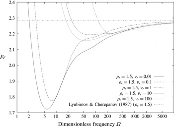
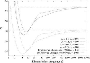
In figures 1 and 2, the dependence of the critical Froude number
 $Fr_{cr}$
on the dimensionless vibration frequency
 $\unicode[STIX]{x1D6FA}$
is presented for
 $\unicode[STIX]{x1D70C}_{r}=1.5$
and different viscosity ratios. As one can see in all cases the dependence is non-monotonic,
 $Fr_{cr}$
decreases with increase of
 $\unicode[STIX]{x1D6FA}$
for low
 $\unicode[STIX]{x1D6FA}$
and grows with
 $\unicode[STIX]{x1D6FA}$
for higher
 $\unicode[STIX]{x1D6FA}$
. At sufficiently high
 $\unicode[STIX]{x1D6FA}$
the growth of
 $Fr_{cr}$
with
 $\unicode[STIX]{x1D6FA}$
slows down and at
 $\unicode[STIX]{x1D6FA}>10^{4}$
the
 $Fr_{cr}(\unicode[STIX]{x1D6FA})$
-curves are close to the asymptote
 $$\begin{eqnarray}\tilde{Fr}_{cr}=\frac{1}{2}\sqrt{\frac{(\unicode[STIX]{x1D70C}_{r}+1)^{3}}{\unicode[STIX]{x1D70C}_{r}(\unicode[STIX]{x1D70C}_{r}-1)}},\end{eqnarray}$$
obtained by Lyubimov & Cherepanov (Reference Lyubimov and Cherepanov1987), using the high-frequency (inviscid) approach. The frequency, at which
 $Fr_{cr}$
attains the asymptotic value, decreases when the viscosity ratio tends to one: it is
 ${\sim}10^{3}$
for
 $\unicode[STIX]{x1D708}_{r}=0.01$
and
 ${\sim}10^{2}$
for
 $\unicode[STIX]{x1D708}_{r}=0.1$
. For the viscosity ratio
 $\unicode[STIX]{x1D708}_{r}=0.01$
the difference between the value of
 $Fr_{cr}$
minimum and asymptotic value is as large as 25 %, and at
 $\unicode[STIX]{x1D708}_{r}=0.1$
it is smaller than 5 %, which suggests that the non-monotonic behaviour is weak. In the low-frequency range, viscosity stabilizes the basic flow by suppressing the longwave perturbations. In contrast to this, under the vibrations of higher frequency at
 $\unicode[STIX]{x1D6FA}>500$
, viscous dissipation exerts just a weak destabilizing effect and the values of
 $Fr_{cr}$
for different
 $\unicode[STIX]{x1D708}_{r}$
are close to each other.
The neutral curves
 $Fr_{cr}(\unicode[STIX]{x1D6FA})$
for
 $\unicode[STIX]{x1D70C}_{r}=1.5$
and different viscosity ratios. The domains below each curve correspond to the stable states with respect to the longwave disturbances and the domains above to the unstable states. The horizontal dashed line is the value predicted by (3.37) from the inviscid theory of Lyubimov & Cherepanov (Reference Lyubimov and Cherepanov1987).

The neutral curves
 $Fr_{cr}(\unicode[STIX]{x1D6FA})$
for
 $\unicode[STIX]{x1D70C}_{r}=1.5$
and
 $\unicode[STIX]{x1D70C}_{r}=2.04$
and different viscosity ratios. The domains below each curve correspond to the stable states with respect to the longwave disturbances and the domains above to the unstable states. The horizontal dashed line is the value predicted by (3.37) from the inviscid theory of Lyubimov & Cherepanov (Reference Lyubimov and Cherepanov1987).

The neutral curves
 $Fr_{cr}(\unicode[STIX]{x1D6FA})$
for
 $\unicode[STIX]{x1D70C}_{r}=1.5$
and
 $\unicode[STIX]{x1D70C}_{r}=2.04$
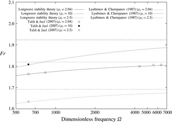
and different viscosity ratios. The domains below each curve correspond to the stable states with respect to the longwave disturbances and the domains above to the unstable states. The horizontal dashed line is the value predicted by (3.37) from the inviscid theory of Lyubimov & Cherepanov (Reference Lyubimov and Cherepanov1987). Points are the values recovered from the plots of Talib & Juel (Reference Talib and Juel2007).

A comparison of the calculated longwave instability thresholds with the results obtained from the inviscid theory of Lyubimov & Cherepanov (Reference Lyubimov and Cherepanov1987) and the data recovered from Talib & Juel (Reference Talib and Juel2007) is given in figure 3. As one can see, our results agree well with the analysis performed by Talib & Juel (Reference Talib and Juel2007). With increasing
 $\unicode[STIX]{x1D6FA}$
the instability curves approach the limit lines obtained in the inviscid case.
4 Transition from the longwave instability to the finite-wavelength instability
As it has been known from the inviscid theory of Lyubimov & Cherepanov (Reference Lyubimov and Cherepanov1987), in thin layers the instability is longwave, and in the layers, the thickness of which exceeds some critical value, the finite-wavelength perturbations are the most dangerous. The formal series expansion in terms of
 $k$
allows us not only to obtain the value of the critical Froude number for longwave perturbations but also to determine whether or not the longwave perturbations could be the most dangerous at certain values of the parameter or, in other words, to determine the sign of the derivative of
 $Re_{cr}$
with respect to
 $k^{2}$
. To this end, it is necessary to consider higher orders of the series expansion with respect to
 $k$
.
Equations (3.2)–(3.4) of the second order are written as
 $$\begin{eqnarray}\displaystyle & \displaystyle \frac{\text{i}}{\unicode[STIX]{x1D70C}}p_{[\pm 1]}^{(2)}\pm \text{i}\unicode[STIX]{x1D6FA}u_{[\pm 1]}^{(2)}-\unicode[STIX]{x1D708}u_{[\pm 1]}^{(2)\prime \prime }=-Re(\text{i}u_{[0]}^{(1)}U_{[\pm 1]}+\text{i}u_{[\pm 2]}^{(0)}U_{[\mp 1]}+w_{[0]}^{(1)}U_{[\mp 1]}^{\prime }+w_{[\pm 2]}^{(1)}U_{[\mp 1]}^{\prime }) & \displaystyle \nonumber\\ \displaystyle & \displaystyle -\,(\unicode[STIX]{x1D708}+\unicode[STIX]{x1D706}^{(2)})u_{[\pm 1]}^{(0)},\,\qquad & \displaystyle\end{eqnarray}$$
 $$\begin{eqnarray}\displaystyle & \displaystyle p_{[\pm 1]}^{(2)\prime }=\unicode[STIX]{x1D70C}(\unicode[STIX]{x1D708}w_{[\pm 1]}^{(1)\prime \prime }\mp \text{i}\unicode[STIX]{x1D6FA}w_{[\pm 1]}^{(1)}), & \displaystyle\end{eqnarray}$$
 $$\begin{eqnarray}\displaystyle & \displaystyle w_{[\pm 1]}^{(2)\prime }+\text{i}u_{[\pm 1]}^{(2)}=0, & \displaystyle\end{eqnarray}$$
with the boundary conditions at
 $z=0$
:
 $$\begin{eqnarray}\displaystyle & \displaystyle [\unicode[STIX]{x1D70C}\unicode[STIX]{x1D708}u_{[\pm 1]}^{(2)\prime }]=-\text{i}[\unicode[STIX]{x1D70C}\unicode[STIX]{x1D708}w_{[\pm 1]}^{(0)}]-\unicode[STIX]{x1D709}_{[0]}^{(2)}[\unicode[STIX]{x1D70C}\unicode[STIX]{x1D708}U_{[\pm 1]}^{\prime \prime }]-\unicode[STIX]{x1D709}_{[\pm 2]}^{(2)}[\unicode[STIX]{x1D70C}\unicode[STIX]{x1D708}U_{[\mp 1]}^{\prime \prime }], & \displaystyle\end{eqnarray}$$
 $$\begin{eqnarray}\displaystyle & \displaystyle [p_{[\pm 1]}^{(2)}]=[\unicode[STIX]{x1D70C}\unicode[STIX]{x1D708}w_{[\pm 1]}^{(0)\prime }]-2\text{i}\unicode[STIX]{x1D709}_{[0]}^{(0)}[\unicode[STIX]{x1D70C}\unicode[STIX]{x1D708}U_{[\pm 1]}^{\prime }]+[\unicode[STIX]{x1D70C}]\frac{Ga}{Re}\unicode[STIX]{x1D709}_{[\pm 1]}^{(1)}, & \displaystyle\end{eqnarray}$$
 $$\begin{eqnarray}\displaystyle & \displaystyle [u_{[\pm 1]}^{(2)}]+\unicode[STIX]{x1D709}_{[0]}^{(2)}[U_{[\pm 1]}^{\prime }]+\unicode[STIX]{x1D709}_{[\pm 2]}^{(2)}[U_{[\mp 1]}^{\prime }]=[w_{[\pm 1]}^{(2)}]=0, & \displaystyle\end{eqnarray}$$
and the no-slip conditions at the rigid walls
 $z=\pm 1/2$
:
 $$\begin{eqnarray}w_{[\pm 1]}^{(2)}=u_{[\pm 1]}^{(2)}=0.\end{eqnarray}$$
The system (4.1)–(4.6) is not closed, since it contains
 $\unicode[STIX]{x1D709}_{[0]}^{(2)}$
. The reason for the appearance of
 $\unicode[STIX]{x1D709}_{[0]}^{(2)}$
is the linearity of perturbations and the possibility of choosing arbitrarily the initial value of the upper index. Indeed, if one seeks a solution for all fields as
 $f=f_{I}(\unicode[STIX]{x1D709}_{[0]}^{(0)})+f_{II}(\unicode[STIX]{x1D709}_{[0]}^{(2)})$
, it is quite obvious that the system determining
 $p_{II[\pm 1]}^{(2)}$
,
 $u_{II[\pm 1]}^{(2)}$
and
 $w_{II[\pm 1]}^{(2)}$
through
 $\unicode[STIX]{x1D709}_{[0]}^{(2)}$
is identical to the system determining
 $p_{I[\pm 1]}^{(0)}$
,
 $u_{I[\pm 1]}^{(0)}$
and
 $w_{I[\pm 1]}^{(0)}$
through
 $\unicode[STIX]{x1D709}_{[0]}^{(0)}$
. In the formal series expansion of the next order, the subsystem, which determines
 $p_{II[\pm 1]}^{(2)}$
,
 $u_{II[\pm 1]}^{(2)}$
and
 $w_{II[\pm 1]}^{(2)}$
in terms of
 $\unicode[STIX]{x1D709}_{[0]}^{(2)}$
, will allow us to express
 $\unicode[STIX]{x1D706}^{(2)}$
in the same way as has been already done in (3.33). Such ‘parasite’, ‘shadow’ subsystems are typical for high-order formal expansion in linear stability problems. Since these subsystems do not contain any useful information, one can simply set
 $\unicode[STIX]{x1D709}_{[0]}^{(2)}=0$
. Then, the system (4.1)–(4.6) becomes closed and
 $p_{[\pm 1]}^{(2)}$
,
 $u_{[\pm 1]}^{(2)}$
and
 $w_{[\pm 1]}^{(2)}$
can be expressed in terms of
 $\unicode[STIX]{x1D709}_{[0]}^{(0)}$
.
In the third-order series expansion, the kinematic condition (3.8) gives
 $$\begin{eqnarray}\unicode[STIX]{x1D706}^{(3)}=0,\quad \unicode[STIX]{x1D709}_{[\pm 1]}^{(3)}=\mp \text{i}\frac{Re}{\unicode[STIX]{x1D6FA}}(w_{[\pm 1]}^{(2)}-\text{i}\unicode[STIX]{x1D709}_{[\pm 2]}^{(2)}U_{[\mp 1]})|_{z=0}\mp \frac{\text{i}}{\unicode[STIX]{x1D6FA}}\unicode[STIX]{x1D706}^{(2)}\unicode[STIX]{x1D709}_{[\pm 1]}^{(1)}.\end{eqnarray}$$
The rest of the system is
 $$\begin{eqnarray}\displaystyle & \displaystyle \unicode[STIX]{x1D708}u_{[0]}^{(3)\prime \prime }-\frac{\text{i}}{\unicode[STIX]{x1D70C}}p_{[0]}^{(3)}-(\unicode[STIX]{x1D708}+\unicode[STIX]{x1D706}^{(2)})u_{[0]}^{(1)}=Q, & \displaystyle\end{eqnarray}$$
 $$\begin{eqnarray}\displaystyle & \displaystyle Q=Re(\text{i}u_{[+1]}^{(2)}U_{[-1]}+\text{i}u_{[-1]}^{(2)}U_{[+1]}+w_{[+1]}^{(2)}U_{[-1]}^{\prime }+w_{[-1]}^{(2)}U_{[+1]}^{\prime }), & \displaystyle\end{eqnarray}$$
 $$\begin{eqnarray}\displaystyle & \displaystyle p_{[0]}^{(3)\prime }=\unicode[STIX]{x1D70C}\unicode[STIX]{x1D708}w_{[0]}^{(1)\prime \prime }-\text{i}\unicode[STIX]{x1D70C}Re(w_{[+1]}^{(0)}U_{[-1]}+w_{[-1]}^{(0)}U_{[+1]}), & \displaystyle\end{eqnarray}$$
 $$\begin{eqnarray}\displaystyle & \displaystyle w_{[0]}^{(3)\prime }+\text{i}u_{[0]}^{(3)}=0, & \displaystyle\end{eqnarray}$$
the boundary conditions on
 $z=0$
are
 $$\begin{eqnarray}\displaystyle & \displaystyle [p_{[0]}^{(3)}]=[\unicode[STIX]{x1D70C}\unicode[STIX]{x1D708}w_{[0]}^{(1)\prime }]-2\text{i}\unicode[STIX]{x1D709}_{[+1]}^{(0)}[\unicode[STIX]{x1D70C}\unicode[STIX]{x1D708}U_{[-1]}^{\prime }]-2\text{i}\unicode[STIX]{x1D709}_{[-1]}^{(0)}[\unicode[STIX]{x1D70C}\unicode[STIX]{x1D708}U_{[+1]}^{\prime }]+[\unicode[STIX]{x1D70C}]\frac{Ga}{ReBo}\unicode[STIX]{x1D709}_{[0]}^{(0)}, & \displaystyle\end{eqnarray}$$
 $$\begin{eqnarray}\displaystyle & \displaystyle [\unicode[STIX]{x1D70C}\unicode[STIX]{x1D708}u_{[0]}^{(3)\prime }]=-\text{i}[\unicode[STIX]{x1D70C}\unicode[STIX]{x1D708}w_{[0]}^{(1)}]-\unicode[STIX]{x1D709}_{[+1]}^{(3)}[\unicode[STIX]{x1D70C}\unicode[STIX]{x1D708}U_{[-1]}^{\prime \prime }]-\unicode[STIX]{x1D709}_{[-1]}^{(3)}[\unicode[STIX]{x1D70C}\unicode[STIX]{x1D708}U_{[+1]}^{\prime \prime }], & \displaystyle\end{eqnarray}$$
 $$\begin{eqnarray}\displaystyle & \displaystyle [u_{[0]}^{(3)}]+\unicode[STIX]{x1D709}_{[+1]}^{(2)}[U_{[-1]}^{\prime }]+\unicode[STIX]{x1D709}_{[-1]}^{(2)}[U_{[+1]}^{\prime }]=[w_{[0]}^{(3)}]=0, & \displaystyle\end{eqnarray}$$
and on the rigid walls
 $$\begin{eqnarray}w_{[0]}^{(3)}|_{z=\pm 1/2}=u_{[0]}^{(3)}|_{z=\pm 1/2}=0.\end{eqnarray}$$
In the fourth-order expansion, the kinematic condition (3.8) is written as
 $$\begin{eqnarray}\unicode[STIX]{x1D706}^{(4)}\unicode[STIX]{x1D709}_{[0]}^{(0)}=Re(w_{[0]}^{(3)}-\text{i}(\unicode[STIX]{x1D709}_{[+1]}^{(3)}U_{[-1]}-\unicode[STIX]{x1D709}_{[-1]}^{(3)}U_{[+1]}))|_{z=0},\end{eqnarray}$$
from which, after excluding the linear multiplication factor
 $\unicode[STIX]{x1D709}_{[0]}^{(0)}$
, we finally arrive at
 $\unicode[STIX]{x1D706}^{(4)}=\unicode[STIX]{x1D706}^{(4)}(Re,\unicode[STIX]{x1D6FA},Ga,\unicode[STIX]{x1D70C}_{r},\unicode[STIX]{x1D708}_{r},Bo)$
. The evaluation of
 $\unicode[STIX]{x1D706}^{(4)}$
using the above formula shows that
 $\unicode[STIX]{x1D706}^{(4)}$
, similarly to
 $\unicode[STIX]{x1D706}^{(2)}$
, is a real value. Thus, in the case when
 $\unicode[STIX]{x1D706}^{(4)}>\unicode[STIX]{x1D706}^{(2)}=0$
an increase in
 $k$
leads to a decrease in
 $Re_{cr}(k)$
. Such behaviour corresponds to the finite-wavelength instability. In the opposite case,
 $\unicode[STIX]{x1D706}^{(4)}<\unicode[STIX]{x1D706}^{(2)}=0$
, the longwave perturbations can be the most dangerous. It is worth mentioning that the minimum of
 $Re_{cr}(k)$
at
 $k=0$
can be local and another global minimum can occur.
The condition
 $\unicode[STIX]{x1D706}^{(4)}=\unicode[STIX]{x1D706}^{(2)}=0$
allows us to determine the function
 $Bo_{cr}=Bo_{cr}(\unicode[STIX]{x1D6FA},Ga,\unicode[STIX]{x1D70C}_{r},\unicode[STIX]{x1D708}_{r})$
, which divides the parameter space into the zones of longwave and finite-wavelength instabilities. For high-frequency small-amplitude vibrations the results of Lyubimov & Cherepanov (Reference Lyubimov and Cherepanov1987) give
 $$\begin{eqnarray}\lim _{\unicode[STIX]{x1D6FA}\rightarrow \infty }Bo_{cr}(\unicode[STIX]{x1D6FA},Ga,\unicode[STIX]{x1D70C}_{r},\unicode[STIX]{x1D708}_{r})=12.\end{eqnarray}$$
The calculations performed by Khenner et al. (Reference Khenner, Lyubimov, Belozerova and Roux1999) for the inviscid case but without limitations on the amplitude give the following expression for the longwave instability zone:
 $$\begin{eqnarray}\left(1-\frac{3}{4}\frac{\unicode[STIX]{x1D70C}_{r}-1}{\unicode[STIX]{x1D70C}_{r}+1}\frac{Ga}{\unicode[STIX]{x1D6FA}^{2}}\right)Bo<12.\end{eqnarray}$$
It follows from this formula that there is a critical value of the dimensionless frequency
 $\unicode[STIX]{x1D6FA}_{cr}$
, below which the longwave instability takes place at any values of the Bond number. For
 $\unicode[STIX]{x1D6FA}>\unicode[STIX]{x1D6FA}_{cr}$
the longwave instability occurs at
 $Bo<Bo_{cr}$
and the finite wavelength instability at
 $Bo>Bo_{cr}$
. At high values of
 $\unicode[STIX]{x1D6FA}$
the value of
 $Bo_{cr}$
is close to the asymptotic value obtained by Lyubimov & Cherepanov (Reference Lyubimov and Cherepanov1987) under the assumption of high-frequency small-amplitude vibrations.
The critical Bond number for
 $\unicode[STIX]{x1D70C}_{r}=1.5$
,
 $Ga=100$
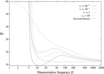
and different viscosity ratios. Below each curve the longwave instability domain is located. The inviscid theory predicts the boundaries between the instability zones according to (4.19).

In figure 4, the dependencies of the critical Bond number on the dimensionless frequency obtained from our calculations are plotted for
 $\unicode[STIX]{x1D70C}_{r}=1.5$
,
 $Ga=100$
and different viscosity ratios. For the comparison the dependence
 $Bo_{cr}(\unicode[STIX]{x1D6FA})$
obtained in Khenner et al. (Reference Khenner, Lyubimov, Belozerova and Roux1999) using the high-frequency (inviscid) finite-amplitude approach is presented in the same figure. As one can see, at
 $\unicode[STIX]{x1D6FA}>10^{3}$
all curves are close to each other and to the asymptote
 $Bo=12$
obtained by Lyubimov & Cherepanov (Reference Lyubimov and Cherepanov1987). In the intermediate frequency range, in contrast to the results of Khenner et al. (Reference Khenner, Lyubimov, Belozerova and Roux1999), the dependencies
 $Bo_{cr}(\unicode[STIX]{x1D6FA})$
are non-monotonic. With further decreasing
 $\unicode[STIX]{x1D6FA}$
the curves
 $Bo_{cr}(\unicode[STIX]{x1D6FA})$
for fluids with
 $\unicode[STIX]{x1D708}_{r}\ll 1$
or
 $\unicode[STIX]{x1D708}_{r}\gg 1$
show a sharp growth at some value of
 $\unicode[STIX]{x1D6FA}$
in the same manner as the dependence (4.19) given in (Khenner et al.
Reference Khenner, Lyubimov, Belozerova and Roux1999). Moreover, the values of
 $\unicode[STIX]{x1D6FA}_{cr}$
for different
 $\unicode[STIX]{x1D708}_{r}$
are close to each other and to (4.19), i.e. for high
 $Ga$
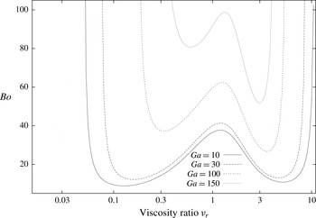
or great contrast of viscosities the longwave instability at low frequencies is most dangerous for any values of the Bond number (see figure 5).
The critical Bond number for
 $\unicode[STIX]{x1D6FA}=0.3$
,
 $\unicode[STIX]{x1D70C}_{r}=1.5$
and different
 $\unicode[STIX]{x1D708}_{r}$
and
 $Ga$
. Below each curve the longwave instability domain is located. As one can see, the curves are qualitatively symmetrical for reverse values of
 $\unicode[STIX]{x1D708}_{r}$
.

However, for fluids with close viscosities and low
 $Ga$
our calculations give qualitatively different behaviour. In this case, in the low-frequency range the dependence
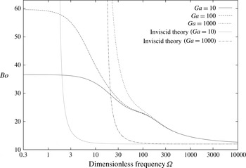
 $Bo_{cr}(\unicode[STIX]{x1D6FA})$
approaches a horizontal asymptote. As one can see from figure 6, this asymptotic value of the critical Bond number decreases with decreasing
 $Ga$
.
The critical Bond number for
 $\unicode[STIX]{x1D70C}_{r}=1.5$
and
 $\unicode[STIX]{x1D708}_{r}=1$
. Each curve corresponds to different
 $Ga$
. Below each curve the longwave instability domain is located. The inviscid theory predicts the boundaries between the instability zones according to (4.19).

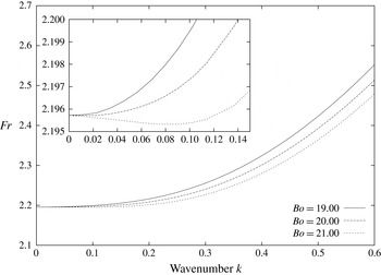
To verify the analytical results for the boundary between the longwave and finite-wavelength instabilities, we carried out numerical calculations for the linear stability problem using finite difference method. In figure 7, the results of these calculations are plotted for the values of the parameters, which are close to the transition boundary:
 $\unicode[STIX]{x1D708}_{r}=1$
,
 $\unicode[STIX]{x1D70C}_{r}=1.5$
,
 $Ga=100$
and
 $\unicode[STIX]{x1D6FA}=200$
. For these parameters the instability is predicted to be longwave if
 $Bo<19.93$
. As one can see, a numerical solution of the linear stability problem confirms the location of the boundary between the longwave and finite-wavelength instabilities.
A change of neutral curves from the cellular to the longwave instability for
 $\unicode[STIX]{x1D708}_{r}=1$
,
 $\unicode[STIX]{x1D70C}_{r}=1.5$
,
 $Ga=100$
and
 $\unicode[STIX]{x1D6FA}=200$
.

As was mentioned above, a positive curvature of the stability curve at
 $k=0$
shows only that the longwave instability can take place and higher-order terms in
 $k$
can lead to a lower threshold at the finite
 $k$
. Therefore, our calculations determine the boundary between the parameter range, in which the finite-wavelength instability is most dangerous and the range, where the longwave instability can be observed. We performed additional numerical calculations for the linear stability problem for a few sets of parameters in a sufficiently wide range of the wavenumber and plotted the neutral curves. For all selected sets of parameters these calculations confirm the longwave type of instability in the domains where the analytical calculations predicted this instability mode.
We also performed a DNS for the onset of instability. The simulation was carried out using the ANSYS Fluent software package, implementing the volume of fluid (VoF) method to describe the dynamics of the interface in a two-layer system. The VoF method is a numerical technique for the investigation of the fluid interface evolution through introducing a volume fraction of each phase. For immiscible fluids the function of the volume fraction is constant inside the selected phase and sharply changes at the interface between the phases. The variables and properties in any given grid cell are either purely representative of one of the phases, or representative of a combination of phases, depending on the values of the volume fraction. Therefore, a multiphase system can be considered as a single medium with sharply changing parameters near the interfaces, and the Navier–Stokes equations describing the system (2.1)–(2.8) can be solved in the same manner over the entire computational domain.
The influence of vibrations was taken into account by introducing a periodically changing volumetric force. The spatial discretization was performed using the third-order MUSCL scheme (Monotone Upstream-Centered Schemes for Conservation Laws). For temporal discretization the first-order scheme was used, but the time step was taken to be much smaller than the period of vibrations, while the frequency of vibrations is quite high. Therefore, the computational error of the first-order scheme was rather small. The no-slip conditions were imposed at the side walls of container.
The calculations were performed for the system of fluids with a large viscosity contrast. In this case, the dynamic boundary layer in one of the liquids is very small and it is important to accurately describe the boundary layer near the fluid interface. Thus, the computational mesh near the interface must be fine enough; we used the dynamic mesh refinement procedure, which significantly reduces the computational time. In order to decrease the effect of sidewalls the calculations were conducted in a rather long cavity, the length of which was 24 times greater than the height. The
 $160\times 960$
computational grid was used. Initially, the fluids fill equal parts of the cavity with a horizontal interface.
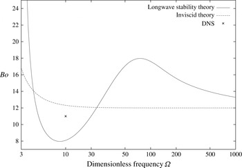
The critical Bond number for
 $\unicode[STIX]{x1D70C}_{r}=2.04$
,
 $\unicode[STIX]{x1D708}_{r}=0.01$
and
 $Ga=10$
. Below each curve the longwave instability domain is located. The inviscid theory predicts the boundaries between the instability zones according to (4.19). The point on the curve corresponds to the performed DNS, which verifies the existence of cellular instability in this zone.

According to (3.14)–(3.24), the first nonzero term in the expression for
 $\unicode[STIX]{x1D706}$
is
 $k^{2}\unicode[STIX]{x1D706}^{(2)}$
, so the characteristic time of the development of longwave instability is proportional to
 $k^{-2}$
. That is why the DNS of the longwave instability is hardly possible: it requires a lot of computational time apart from a large computational domain. Because of this, the verification of the analytical results was carried out for the region of transition from the longwave instability to the finite-wavelength one. We selected a set of parameters, for which the inviscid theory predicts the longwave instability, and our viscous analysis predicts the instability with respect to finite-wavelength perturbations. The dimensionless parameters corresponding to this situation are
 $Re=4.45$
,
 $\unicode[STIX]{x1D708}_{r}=0.01$
,
 $\unicode[STIX]{x1D70C}_{r}=2.04$
,
 $Ga=10$
,
 $\unicode[STIX]{x1D6FA}=10$
and
 $Bo=11$
(see figure 8). The Froude number corresponding to these parameters,
 $Fr=Re/\sqrt{Ga}=1.407$
, is smaller than the threshold of longwave instability predicted by the asymptotic theory,
 $Fr_{cr}=1.434$
(see figure 2).
The frozen wave in the middle part of the cavity for
 $Re=4.45$
,
 $\unicode[STIX]{x1D708}_{r}=0.01$
,
 $\unicode[STIX]{x1D70C}_{r}=2.04$
,
 $Ga=10$
,
 $\unicode[STIX]{x1D6FA}=10$
and
 $Bo=11$
.

The calculations show the occurrence of the frozen wave, i.e. the instability is of the finite-wavelength type (the shape of the interface is shown in figure 9). Since the examined Froude number is smaller than the threshold predicted by the asymptotic theory, we can conclude that the results of DNS substantiate the results obtained in the present paper.
5 Conclusion
In this paper, we studied the effect of viscosity contrast on the development of the longwave instability in a two-layer system subjected to horizontal vibrations. It was demonstrated that viscosity contrast exerts a significant influence on the longwave instability threshold. Although these effects were already discussed in Talib & Juel (Reference Talib and Juel2007), the present investigation shows more clearly how the viscosity ratio of two fluids modifies the critical vibration parameters and provides supporting evidence for the dominance of the longwave instability.
The analysis showed, that at low frequencies, viscosity suppresses the longwave perturbations and as a result has a strong stabilizing effect on the basic flow. In contrast to this, for vibrations of high frequency the viscous dissipation exerts a weak destabilizing effect. At moderate vibration frequencies, the destabilizing effect of viscosity is more significant; the critical value of the vibration velocity amplitude strongly decreases. This effect is especially strong in systems with large viscosity contrast.
Usually, both the surface tension and viscosity suppress the short-wave perturbations, whereas the longwave perturbations are less affected by these factors. However, the calculation of the boundary separating the longwave and finite-wavelength instability domains in the parameter space predicted the longwave instability at high viscosities regardless of the surface tension. At sufficiently low vibration frequencies the suppression of the finite-wavelength perturbations by viscosity can be so strong that the longwave Kelvin–Helmholtz perturbations become the most dangerous at any values of the surface tension coefficient. The results obtained in the present paper led us to the conclusion that the development of the longwave Kelvin–Helmholtz instability under vibrations of finite frequencies can take place in thick fluid layers or even in layers of arbitrary thickness if viscosities of the fluids are high.
The surprising finding is that at finite frequencies the critical Bond number can be lower than the prediction of the inviscid theory. The suppressing effect of capillarity and viscous dissipation are supposed to be far stronger for the perturbations with finite wavelength than for the longwave perturbations. However, the calculations showed that at finite frequencies there exists a parameter domain, in which viscosity weakens the influence of the capillary forces, making finite-wavelength instability more dangerous than the longwave one. Such an effect can only be observed in the case of large viscosity contrast.
Acknowledgements
This work was carried out under financial support from the Russian Science Foundation (grant no. 14-21-00090). The authors are grateful to S. V. Shklyaev for interesting and productive discussions.