2. Formulation

2.1. MHD equations

Compressible MHD equations are

(2.1)\begin{gather} \partial_t \rho + \boldsymbol{\nabla} \boldsymbol{\cdot} \left(\rho \boldsymbol{u}\right) = 0, \end{gather}

(2.2)\begin{gather} \partial_t \left(\rho \boldsymbol{u}\right) + \boldsymbol{\nabla} \boldsymbol{\cdot} \left[\rho \boldsymbol{uu} + p \boldsymbol{\mathsf{I}}+ {\tfrac{1}{2}}\left(\boldsymbol{b}^2\right) \boldsymbol{\mathsf{I}}- \boldsymbol{bb} \right] = \boldsymbol{\nabla} \boldsymbol{\cdot} \boldsymbol{\sigma}, \end{gather}

(2.3)\begin{gather} \partial_t \boldsymbol{b} + \boldsymbol{\nabla} \boldsymbol{\cdot} \left(\boldsymbol{u} \boldsymbol{b}-\boldsymbol{b} \boldsymbol{u}\right) = \eta {\nabla^2}\boldsymbol{b}, \end{gather}

(2.4)\begin{gather} \partial_t \mathcal{E} + \boldsymbol{\nabla}\boldsymbol{\cdot} \left[\left(\mathcal{E}+p+{\tfrac{1}{2}}\boldsymbol{b}^2\right) \boldsymbol{u} - \left(\boldsymbol{bb}\right) \boldsymbol{\cdot} \boldsymbol{u} \right] \nonumber\\ \quad= {\boldsymbol{\nabla}\boldsymbol{\cdot} \left(\kappa \boldsymbol{\nabla} T\right)} + \boldsymbol{\nabla}\boldsymbol{\cdot} \left(\boldsymbol{\sigma} \boldsymbol{\cdot} \boldsymbol{u} \right) + \boldsymbol{\nabla} \boldsymbol{\cdot} \left[\boldsymbol{b} \times (\eta \boldsymbol{\nabla} \times \boldsymbol{b}) \right], \end{gather}

where $\rho$, $\boldsymbol {u}$, $p$, $T$, $\boldsymbol {b}$ and $\mathcal {E}=\rho \boldsymbol {u}\boldsymbol {\cdot }\boldsymbol {u}/2+p/(\gamma -1)+\boldsymbol {b} \boldsymbol {\cdot } \boldsymbol {b}/{2}=E_k+E_{th}+E_b$ denote density, velocity, pressure, temperature, magnetic field and total (kinetic, thermal and magnetic) energy. $\gamma$ is the adiabatic index with a value, $\gamma =1.4$; $\boldsymbol{\mathsf{I}}$ is the unity tensor; $\sigma _{ij}=\mu (\partial _i u_j + \partial _j u_i)-2(\mu (\boldsymbol {\nabla } \boldsymbol {\cdot } \boldsymbol {u}) \delta _{ij})/3$ is the viscous stress tensor; $\mu$ is the dynamic viscosity; $\eta$ is the magnetic diffusivity; and $\kappa$ is the thermal conductivity. The MHD equations are closed with the equation of state of an ideal gas. This set of compressible MHD equations is expected to be valid in a conducting ideal gas such as a hydrogen plasma when collisions are dominant and the medium is isotropic so that the dissipation coefficients are scalars.

The MHD equations are non-dimensionalized by introducing several reference scales. For example, length is normalized to $L_0$, velocity to $U_0$, density to $\rho _0$, magnetic field to $B_0$, temperature to $T_0$, viscosity to $\mu _0$, magnetic diffusivity to $\eta _0$ and thermal conductivity to $\kappa _0$. Then the system is control by several dimensionless parameters, such as the Reynolds number $Re=\rho _0 U_0 L_0/\mu _0$, the magnetic Reynolds number $Re_m=U_0 L_0/\eta _0$ and the Mach number $M=U_0/c_{s,0}$, where $c_{s,0}=\sqrt {\gamma R T_0}$ is the reference sound speed and $R$ is the universal gas constant. The dimensionless $\mu$, $\kappa$ and $\eta$ (here we use the same symbols as dimensional ones without confusion) are assumed to be described by the Sutherland's law as used by Yang et al. (Reference Yang, Wan, Shi, Yang and Chen2016b), $\mu =\kappa =\eta =1.4042T^{3/2}/(T+0.4042)$.

2.2. Helmholtz decomposition

To clarify the interchange among differing components, the Helmholtz decomposition is employed (as used in Kida & Orszag Reference Kida and Orszag1992; Miura & Kida Reference Miura and Kida1995; Pan & Johnsen Reference Pan and Johnsen2017) to separate compressible and incompressible motions of the velocity field. It can be applied to the Fourier transform $\hat {\boldsymbol {v}}(\boldsymbol {k})$ of any vector field $\boldsymbol {v}(\boldsymbol {x})$ of zero mean, which decomposes $\hat {\boldsymbol {v}}$ into components along and normal to $\boldsymbol {k}$

(2.5)\begin{equation} \hat{\boldsymbol{v}}=\hat{\boldsymbol{v}}_c + \hat{\boldsymbol{v}}_s, \end{equation}

where $\hat {\boldsymbol {v}}_c={\boldsymbol {k} (\boldsymbol {k} \cdot \hat {\boldsymbol {v}})}/{k^2}$ is the compressive (longitudinal) part and $\hat {\boldsymbol {v}}_s=-({\boldsymbol {k} \times (\boldsymbol {k} \times \hat {\boldsymbol {v}})}/{k^2})$ is the solenoidal (transverse) part. After accomplishing this separation, it is straightforward to reassemble the velocity in real space (or Fourier-space) into incompressible and compressible parts. For flows that are potentially strongly compressive, it is convenient to gauge the relative amplitudes of these motions with a density weighting. We introduce a variable $\boldsymbol {w}=\sqrt {\rho } \boldsymbol {u}$. The r.m.s. value of the compressive part of $\boldsymbol {w}$ will be written as the longitudinal part $u_L$, while the r.m.s. value of the solenoidal part of $\boldsymbol {w}$ is designated as the transverse part $u_T$. In general this differs slightly from the decomposition of the velocity itself into transverse and longitudinal parts, as has been customary in the theory of nearly incompressible flows (Klainerman & Majda Reference Klainerman and Majda1982; Matthaeus & Brown Reference Matthaeus and Brown1988; Ghosh & Matthaeus Reference Ghosh and Matthaeus1992). However in the limit of low Mach number and incompressibility the two approaches coincide. With these definitions, the kinetic energy can be decomposed into compressive and solenoidal parts as follows.

From (2.1) and (2.2), we have

(2.6)\begin{equation} \partial_t \boldsymbol{w} = \boldsymbol{A} + \boldsymbol{P} + \boldsymbol{M} + \boldsymbol{D}, \end{equation}

where

(2.7)\begin{gather} \boldsymbol{A}={-}\left[(\boldsymbol{u} \boldsymbol{\cdot} \boldsymbol{\nabla}) \boldsymbol{w} + {\tfrac{1}{2}} \boldsymbol{w} \boldsymbol{\nabla} \boldsymbol{\cdot} \boldsymbol{u}\right], \end{gather}

(2.8)\begin{gather}\boldsymbol{P}={-}{\frac{\boldsymbol{\nabla} p}{\sqrt{\rho}}}, \end{gather}

(2.9)\begin{gather}\boldsymbol{M}={\frac{(\boldsymbol{\nabla}\times \boldsymbol{b})\times \boldsymbol{b}}{\sqrt{\rho}}}={-} \frac{\boldsymbol{\nabla}(\boldsymbol{b}^2/2)}{\sqrt{\rho}}+\frac{(\boldsymbol{b}\boldsymbol{\cdot}\boldsymbol{\nabla}) \boldsymbol{b}}{\sqrt{\rho}}, \end{gather}

(2.10)\begin{gather}\boldsymbol{D}={\frac{\boldsymbol{\nabla}\boldsymbol{\cdot} \boldsymbol{\sigma}}{\sqrt{\rho}}}. \end{gather}

Note that the Lorentz force $\boldsymbol {M}$ is composed of magnetic pressure term, $\boldsymbol {M}_1=-{\boldsymbol {\nabla }(\boldsymbol {b}^2/2)}/{\sqrt {\rho }}$ and remaining stress term $\boldsymbol {M}_2={(\boldsymbol {b}\boldsymbol {\cdot }\boldsymbol {\nabla })\boldsymbol {b}}/{\sqrt {\rho }}$. Accordingly, the evolution of the decomposed kinetic energy spectra can be derived from (2.6) as

(2.11)\begin{equation} \partial_t E_{k,\alpha}(k,t)=A_{\alpha}(k,t) + P_{\alpha}(k,t) + M_{\alpha}(k,t) + D_{\alpha}(k,t), \end{equation}

where the subscript $\alpha =c, s$ represents compressive and solenoidal parts, respectively.

(2.12)\begin{gather} E_{k,\alpha}(k,t)=\sum_{k-0.5\leqslant|\boldsymbol{k} |< k+0.5} \tfrac{1}{2} \hat{\boldsymbol{w}}_{\alpha}(\boldsymbol{k},t) \cdot \hat{\boldsymbol{w}}_{\alpha}^*(\boldsymbol{k},t), \end{gather}

(2.13)\begin{gather}A_{\alpha}(k,t)= \sum_{k-0.5\leqslant|\boldsymbol{k}| < k+0.5} \hat{\boldsymbol{w}}_{\alpha}^*(\boldsymbol{k},t) \cdot \hat{\boldsymbol{A}}_{\alpha}(\boldsymbol{k},t), \end{gather}

(2.14)\begin{gather}P_{\alpha}(k,t)= \sum_{k-0.5\leqslant|\boldsymbol{k}| < k+0.5} \hat{\boldsymbol{w}}_{\alpha}^*(\boldsymbol{k},t) \cdot \hat{\boldsymbol{P}}_{\alpha}(\boldsymbol{k},t), \end{gather}

(2.15)\begin{gather}M_{\alpha}(k,t)= \sum_{k-0.5\leqslant|\boldsymbol{k}| < k+0.5} \hat{\boldsymbol{w}}_{\alpha}^*(\boldsymbol{k},t)\cdot \hat{\boldsymbol{M}}_{\alpha}(\boldsymbol{k},t), \end{gather}

(2.16)\begin{gather}D_{\alpha}(k,t)= \sum_{k-0.5\leqslant|\boldsymbol{k}| < k+0.5} \hat{\boldsymbol{w}}_{\alpha}^*(\boldsymbol{k},t) \cdot \hat{\boldsymbol{D}}_{\alpha}(\boldsymbol{k},t). \end{gather}

Summing (2.11) over all shells yields the evolution of spatially averaged kinetic energy, $\langle E_{k,\alpha }\rangle (t)=\sum _k E_{k,\alpha }(k,t)$, with spatial averages of the quantities in (2.12)–(2.16) analogously defined,

(2.17)\begin{equation} \partial_t \langle E_{k,\alpha}\rangle= \langle A_{\alpha}\rangle + \langle P_{\alpha}\rangle + \langle M_{\alpha}\rangle + \langle D_{\alpha}\rangle. \end{equation}

In this equation we identify the various terms as

1. (i) $\langle A_{\alpha } \rangle$ is the advection term that exchanges kinetic energy between compressive and solenoidal types. $\langle A_{c} \rangle +\langle A_{s} \rangle$=0 for periodic boundary condition.

2. (ii) $\langle P_{\alpha }\rangle$ is the pressure-dilatation term that exchange energy between type $\alpha$ kinetic and thermal components.

3. (iii) $\langle M_{\alpha }\rangle$ is the Lorentz force term that represents the exchange of type $\alpha$ kinetic and magnetic energy.

4. (iv) $\langle D_{\alpha }\rangle$ is the viscous dissipation term of kinetic energy of type $\alpha$.

In summary, we focus on four types of energy: solenoidal kinetic energy $\langle E_{k,s}\rangle$, compressive kinetic energy $\langle E_{k,c}\rangle$ (as defined in (2.17)), magnetic energy $\langle E_b\rangle =\langle \boldsymbol {b} \boldsymbol {\cdot } \boldsymbol {b}/2\rangle$ and thermal energy $\langle E_{th}\rangle =\langle p/(\gamma -1)\rangle$, and the channels in (2.17) concerning their exchange.

3. Simulation details

We solve the compressible MHD equation via a hybrid scheme (Yang et al. Reference Yang, Wan, Shi, Yang and Chen2016b; Yang Reference Yang2019), which couples a sixth-order compact finite difference scheme for smooth regions and a fifth-order weighted essentially non-oscillatory (WENO) scheme for shock regions. The fields are advanced in time by a third-order Runge–Kutta method. All runs discussed here are freely decaying initial value problems conducted in periodic $(2{\rm \pi} )^3$ geometry with $512^3$ grid points. The magnetic Prandtl number is $Pm = 1$, and we do not impose an external magnetic field. All runs have initially uniform density and temperature. The velocity and magnetic fields are initialized at Fourier modes $1\leqslant |\boldsymbol {k}| \leqslant 8$ with random phases, and with modal spectra proportional to ${1}/[1+(k/k_c)^{8/3}]$ with $k_c=3$. The initial cross helicity, $H_c=2\langle \boldsymbol {u} \cdot \boldsymbol {b}\rangle /\langle \boldsymbol {u}^2+ \boldsymbol {b}^2\rangle$, though not exactly zero, is very small.

To study the energy transfer among solenoidal kinetic $\langle E_{k,s}\rangle$, compressive kinetic $\langle E_{k,c}\rangle$, magnetic $\langle E_b\rangle$ and thermal energy $\langle E_{th}\rangle$, we initialize our system with a range of Mach numbers and a variety of initial velocity and magnetic fluctuations. These runs are grouped into four series that respectively emphasize time variations of these four types of energy. We briefly summarize these runs in the following, and more details are listed for each run in table 1. Note that the Taylor-scale Reynolds number $Re_{\lambda }$, which is always used to compare the turbulence between different flows, is defined as

(3.1)\begin{equation} Re_{\lambda}=Re \frac{u_{rms}\lambda \rho}{\mu}, \end{equation}

where $u_{rms}=\sqrt {\langle \boldsymbol {u}\cdot \boldsymbol {u}\rangle /{3}}$ is the r.m.s velocity, $\lambda =u_{rms}/\omega _{rms}$ is the Taylor microscale and $\omega _{rms}$ is the r.m.s. value of vorticity $\boldsymbol {\omega }=\boldsymbol {\nabla } \times \boldsymbol {u}$. The turbulent Mach number $M_t$, related to compressibility in some sense, is defined as

(3.2)\begin{equation} M_t=M \frac{\sqrt{\langle \boldsymbol{u}\cdot \boldsymbol{u}\rangle}}{\sqrt{T}}, \end{equation}

where $T$ is the temperature. Varying velocity field could result in different $Re_{\lambda }$ and $M_t$ as listed in table 1. The large-eddy turnover times for the runs are different and vary with time (initial large-eddy turnover time ${\sim }2.0$), so the time throughout the paper will be in code units.

Table 1.

Simulation parameters: grid size $N^3$, initial turbulent Mach number $M_t=M (\sqrt {\langle \boldsymbol {u}\cdot \boldsymbol {u}\rangle }/\sqrt {T})$ where $T$ is the temperature, initial Taylor-scale Reynolds number $Re_{\lambda }=Re ({u_{rms}\lambda \rho }/{\mu })$ where $u_{rms}$ is the r.m.s. velocity and $\lambda$ is the Taylor microscale, initial solenoidal kinetic, compressive kinetic and magnetic energy $\langle E_{k,s} \rangle _0, \langle E_{k,c} \rangle _0, \langle E_{b} \rangle _0$. Note that T03 and S05 runs are the same.

The first series of runs, listed as Type T in table 1, emphasizes energy interchange between compressive kinetic energy and thermal components, here commencing with equal amplitude of compressive velocity field energy and magnetic energy, $\langle E_{k,c}\rangle _0=\langle E_b \rangle _0=0.5$ and an absence of a solenoidal kinetic energy component. Three values of initial turbulent Mach number $M_t=0.1, 0.5, 1.0$ are used.

The second series of runs, Type S, are similar to the first series of type T runs in that only the compressive kinetic and magnetic components are excited, but with varying amplitudes ranging from $0.0$ to $0.5$. These runs are intended to clarify which energy reservoir is the main contributor to supplying solenoidal kinetic energy.

The third series of runs have varying turbulent Mach numbers and amplitudes of solenoidal kinetic and magnetic energy. This series of runs is devised to study the growth of compressive kinetic energy and its dependence on Mach number, which are referred to as type C.

Runs in the fourth series are initialized with a mixture of solenoidal and compressive kinetic components. Note that the compressible MHD with quite a small initial magnetic energy behaves like compressible hydrodynamics, e.g. S09 and C04, since the magnetic energy tends to dissipate out of the system rapidly, without substantially interacting with the kinetic part. Therefore, a small amount of magnetic energy is introduced in the beginning to avoid reducing immediately to hydrodynamic-like dynamics and, at the same time, to address questions concerning magnetic field amplification (dynamo). We refer to this set of runs as type B.

To quantify the contribution from solenoidal kinetic energy to magnetic energy, we make a specific comparison to type B runs by introducing a series of incompressible runs labelled as type I. We numerically solve the incompressible MHD equations (see appendix A) in periodic $(2{\rm \pi} )^3$ geometry using the standard pseudo-spectral method with de-aliasing by the two-thirds rule. The fields are advanced in time by a second-order Adam–Bashforth scheme. All other parameters are set up in the same way as the compressible runs. In table 1 we show the initial kinetic energy at changing its amplitude from $0.15$ to $0.5$. We do not conduct a corresponding incompressible run to B05 since its initial state is nearly uniform and still.

4. Acoustic energy exchange

Here, we consider the energy exchange between compressive kinetic and thermal components. Based on (2.17), it is clear that the pressure dilatation and the viscous dissipation are two alternatives that can couple kinetic and thermal energy. But unlike the viscous dissipation, the point-wise pressure dilatation is not positive definite. We expect that the pressure dilatation exchanges energy between solenoidal kinetic and thermal forms at a significantly diminished level, since this term arises mainly from compressibility effects. Therefore, we focus on type T runs in this section, which are initialized with purely compressible motion to generate as strongly compressed flows as possible.

We proceed with the T01 run at low initial turbulent Mach number $M_t=0.1$. The time histories of solenoidal kinetic, compressive kinetic, magnetic and thermal energy are shown in figure 1. The total (kinetic, thermal and magnetic) energy is conserved. The thermal energy $\langle E_{th} \rangle$ keeps increasing on average partially due to the energy supply from kinetic and magnetic energy through viscous and resistive dissipation. Also noteworthy, is the regular oscillation in compressive kinetic and thermal energy, while solenoidal kinetic and magnetic energy varies with time smoothly. It is widely recognized that compressive velocity field is inherently wave-like and thus associated with oscillatory characters. Similar oscillations have been reported in compressible hydrodynamic turbulence (Kida & Orszag Reference Kida and Orszag1992; Sarkar Reference Sarkar1992; Miura & Kida Reference Miura and Kida1995; Ristorcelli Reference Ristorcelli1997; Lee, Yu & Girimaji Reference Lee, Yu and Girimaji2006; Pan & Johnsen Reference Pan and Johnsen2017; Praturi & Girimaji Reference Praturi and Girimaji2019), which is attributed to the pressure-dilatation term $\langle P_c\rangle$. It is natural to expect that this reasoning is still applicable to our cases, even though both pressure and dilatation might be affected by the magnetic field. One may recall that the interference of linear Alfvén waves could lead to oscillatory exchanges between kinetic and magnetic energies (Pouquet, Sulem & Meneguzzi Reference Pouquet, Sulem and Meneguzzi1988). The Alfvén speed is much smaller than the sound speed here, thus merely introducing minor effects on the wavelike character. We show the time history of pressure dilatation in figure 2. The solenoidal part of pressure dilatation $\langle P_s \rangle$ is negligible, while the compressive part $\langle P_c \rangle$ evidently exhibits oscillations. Although the time history of the pressure dilatation is not sign-definite, as energy may be transferred into or out of thermal energy, its time integral indicates net transfer into thermal energy.

Figure 1.

Time histories of solenoidal kinetic $\langle E_{k,s}\rangle$, compressive kinetic $\langle E_{k,c} \rangle$, magnetic $\langle E_b \rangle$ and thermal energy $\langle E_{th}\rangle$ for T01 run. The change in thermal energy from its initial value $\varDelta \langle E_{th} \rangle$ is plotted. The total energy (sum of the four energies in the plot) $\langle E_{tot}\rangle$ is conserved.

Figure 2.

Time evolutions of solenoidal $\langle P_s\rangle$ and compressive parts $\langle P_c\rangle$ of pressure dilatation and its time integral for T01 run.

The results at higher Mach number are shown in figure 3, where one can see slight evolutionary differences in magnetic and solenoidal kinetic energy, while compressive kinetic and thermal energy oscillate with distinct periods. A higher Mach number leads to longer periods of the oscillation; this is quantitatively listed in table 2. Also listed is an estimated period from linear theory $\tau _{linear}={\rm \pi} /c_s$ ($c_s$ is the sound speed), which agrees well with the period from the simulation $\tau$. This suggests that acoustic waves take part in the compressible kinetic-thermal energy exchange channel. The procedure for estimating the period is detailed in the following.

Figure 3.

Time histories of magnetic $\langle E_b \rangle$, solenoidal kinetic $\langle E_{k,s} \rangle$, compressive kinetic $\langle E_{k,c} \rangle$ and thermal energy $\langle E_{th} \rangle$ in type T runs with initial turbulent Mach number $M_t=0.1, 0.5, 1.0$. The change in thermal energy from its initial value $\varDelta \langle E_{th} \rangle$ is plotted.

Table 2.

Initial turbulent Mach number $M_t$, time averaged sound speed $c_s$,$^{a}$ period of oscillations $\tau$ and period of oscillations estimated from linear theory $\tau _{linear}={\rm \pi} /c_s$.

$^{a}$The sound speed increases slightly with time in these simulations.

We consider the simplest case of homogeneous compressible MHD described by $\rho _0$, $p_0$, $\boldsymbol {u}_0$ and $\boldsymbol {b}_0$. The initial uniform state is $\rho _0=1$, $\boldsymbol {u}_0=0$ and $\boldsymbol {b}_0=0$. For sufficiently small perturbations, $\rho '$, $p'$, $\boldsymbol {u}'$ and $\boldsymbol {b}'$, we can linearize the MHD equations (2.2) and (2.4) as

(4.1)\begin{gather} \partial_t \boldsymbol{u}' ={-}\boldsymbol{\nabla} p', \end{gather}

(4.2)\begin{gather}\partial_t p' ={-} \gamma p_0 \boldsymbol{\nabla} \boldsymbol{\cdot} \boldsymbol{u}', \end{gather}

neglecting diffusive processes for simplicity. These equations can be reduced to a single one for $p'$:

(4.3)\begin{equation} \frac{\partial^2 p'}{\partial t^2} = c_s^2 \nabla^2 p', \end{equation}

which can be written in Fourier space as

(4.4)\begin{equation} \frac{\partial^2 \widehat{p'}(\boldsymbol{k},t)}{\partial t^2} ={-}c_s^2 k^2 \widehat{p'}(\boldsymbol{k},t). \end{equation}

The solution to this wave equation is a combination of wave functions,

(4.5)\begin{equation} \widehat{p'}(\boldsymbol{k},t)= A \ \textrm{e}^{-\textrm{i} c_s k t} +B \ \textrm{e}^{\textrm{i} c_s k t},\end{equation}

where complex numbers $A, B$ depend on initial and boundary conditions. Velocity fluctuation $\boldsymbol {u}'$ is obtained by substituting (4.5) for $p'$ in (4.1). Then the pressure dilatation term is

(4.6)\begin{equation} P(k,t)=\sum_{1-0.5\leqslant|\boldsymbol{k}|<1+0.5} \frac{2k}{c_s} \textrm{Im}(A^* B \ \textrm{e}^{2\textrm{i} c_s k t}). \end{equation}

A similar expression has been obtained by Miura & Kida (Reference Miura and Kida1995).

The period of oscillation is different at different wave numbers, but that of compressive kinetic energy is determined by the smallest wavenumber ($k=1$), which is the dominant mode in our cases, as shown in figure 4. At the smallest wavenumber ($k=1$),

(4.7)\begin{equation} P(k=1,t)=\sum_{1-0.5\leqslant|\boldsymbol{k}|<1+0.5} \frac{2}{c_s} \textrm{Im}(A^* B \ \textrm{e}^{2\textrm{i} c_s t}). \end{equation}

The period of oscillation estimated from the linear theory is $\tau _{linear}={\rm \pi} /c_s$.

Figure 4.

Time history of compressive kinetic energy at different wavenumbers for T03 run.

5. Energy transfer among kinetic and magnetic components

We consider the energy interchange among solenoidal kinetic, compressive kinetic and magnetic components through the advection term $\langle A_{\alpha } \rangle$ and the Lorentz force term $\langle M_{\alpha } \rangle$, where again, $\alpha = c$ or $s$ indicates compressive or solenoidal contributions respectively. Figure 5 shows Run S05 as an example. One can see that these terms vary at early times and approach zero asymptotically. This indicates that global exchange between kinetic and magnetic energy is negligible after adjustments that occur during the first few characteristic times.

Figure 5.

Time variations of the solenoidal part of the advection term $\langle A_{s} \rangle$ and the solenoidal and compressive part of the Lorentz force term $\langle M_{s} \rangle$ and$\langle M_{c} \rangle$ in Run S05 as an example.

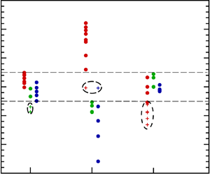
Figure 6 shows the time integrals of the advection term and the solenoidal and compressive parts of the Lorentz force term for all the examined runs. Note that the integral, denoted by $\int \cdot \,\textrm {d}t$, is taken from $t=0$ to the end of runs, i.e. $t=10.0$ in our code unit. For most of the runs, a prominent feature is the dominance of the solenoidal part of the Lorentz force term $\int \langle M_{s} \rangle \,\textrm {d}t$, accounting for the energy exchange between solenoidal kinetic and magnetic components. One can see that values of the advection term $\int \langle A_{s} \rangle \,\textrm {d}t$, and the compressive part of the Lorentz force term $\int \langle M_{c} \rangle \,\textrm {d}t$, mainly reside in the range $[-0.05, 0.05]$, while the magnitude of the solenoidal part $\int \langle M_{s} \rangle \,\textrm {d}t$ is primarily larger than $0.05$. To clarify this point quantitatively, we list these values for some runs in table 3. For example, in Run S01, $\int \langle M_{s} \rangle \,\textrm {d}t=0.16$ and $\int \langle M_{c} \rangle \,\textrm {d}t=0.033$ indicates that a larger fraction of released magnetic energy is converted into solenoidal kinetic energy, as opposed to compressive kinetic energy. Similarly in Run B01, $\int \langle A_{s} \rangle \,\textrm {d}t=-0.049$ and $\int \langle M_{s} \rangle \,\textrm {d}t=-0.26$ indicates that solenoidal kinetic energy is mainly converted into magnetic energy, while less is converted into compressive kinetic energy. In Run S05, magnetic energy is the main contributor to solenoidal kinetic energy. Conversely, run B03 indicates that solenoidal kinetic energy is the main contributor to magnetic energy. Taken together these runs also support the aforementioned conjecture, that conversion between magnetic energy and flow kinetic energy occurs more readily through couplings that involve the solenoidal part of the flow. There is no clear trend of the relative strength of the compressible kinetic-magnetic exchange $\int \langle M_{c} \rangle \,\textrm {d}t$ and the solenoidal-compressive kinetic exchange $\int \langle A_{s} \rangle \,\textrm {d}t$, as shown in figure 6; see also Runs B05 and C02 in table 3.

Figure 6.

Time integrals (from $t=0$ to the end of runs) of the advection term $\langle A_{s} \rangle$ and the solenoidal and compressive parts of the Lorentz force term $\langle M_{s} \rangle$ and $\langle M_{c} \rangle$ for all type S, C and B runs.

Table 3.

Selected Runs discussed in Section V. Initial solenoidal kinetic, compressive kinetic and magnetic energy $\langle E_{k,s} \rangle _0, \langle E_{k,c} \rangle _0, \langle E_{b}\rangle _0$ and time integrals of the solenoidal part of the advection term $\int \langle A_{s} \rangle \,\textrm {d}t$ and the solenoidal and compressive parts of the Lorentz force term $\int \langle M_{s} \rangle \,\textrm {d}t$ and $\int \langle M_{c} \rangle \,\textrm {d}t$.

The outliers are marked by crosses in figure 6, which may seem at first to be in conflict with the point above. But it is maybe not so surprising as we look into these simulations. We take Run B05 as an example, whose $\int \langle M_{s} \rangle \,\textrm {d}t$ is rather small. Note that neither solenoidal kinetic energy nor a large amount of magnetic energy was introduced initially in Run B05, for which it is reasonable to expect that the interaction between solenoidal kinetic and magnetic components through $\int \langle M_{s} \rangle \,\textrm {d}t$ is negligible. With these specific cases in mind, we can make the point that the solenoidal kinetic-magnetic exchange is more efficient than two other available channels, i.e. the solenoidal-compressive kinetic exchange and the compressive kinetic-magnetic exchange. Evidently the interactions of the magnetic field with the compressive flows are mainly oscillatory, in the sense of magnetosonic modes, and tend to rapidly average to small values. The stronger, more secular changes in the energy balance with the magnetic field are mediated more effectively by the solenoidal flow.

6. Short-time energy amplification

While energy decay has been previously studied in the context of hydrodynamic and magnetohydrodynamic turbulence, a common feature among many of these studies is the focus on long time asymptotic behaviours. In this section, we instead describe global turbulent processes operating on short time scales. Point-wise relaxation at short time scales has been discussed in Servidio, Matthaeus & Dmitruk (Reference Servidio, Matthaeus and Dmitruk2008).

6.1. Solenoidal kinetic energy amplification

Note that no solenoidal kinetic energy is initially excited in the series of Type S runs. One may anticipate that a certain amount of solenoidal kinetic energy may be developed at some later time. Indeed, it is reported in Stribling & Matthaeus (Reference Stribling and Matthaeus1991) that the incompressible MHD system in which kinetic and magnetic energies are initially of greatly different magnitudes can evolve rapidly towards near-equipartition of kinetic and magnetic energies. This tendency towards order-one equipartition is sometimes called the ‘Alfvén effect’ (Fyfe, Montgomery & Joyce Reference Fyfe, Montgomery and Joyce1977) and is widely invoked in astrophysics. For the compressible MHD system presented here, figure 7 shows the time evolution of solenoidal kinetic energy. One can see that the solenoidal kinetic energy $\langle E_{k,s}\rangle$ grows rapidly in each type S run, even though it is absent initially, and reaches its maximum at different levels before decay begins.

Figure 7.

Time variation of solenoidal kinetic energy in type S runs, which initially lack solenoidal flows.

The time for $\langle E_{k,s} \rangle$ to reach maximum, $t_{max}$, is listed in table 4. For each of the runs, $t_{max} \sim 1$, which is smaller than initial large-eddy turnover time. The maxima of solenoidal kinetic energy are plotted in figure 8 as a function of initial compressive kinetic or magnetic energies for all type S runs. Two branches appear, one (top branch) with fixed $\langle E_b \rangle _0=0.5$ and varying $\langle E_{k,c}\rangle _0$ from $0.0$ to $0.5$, and the other (bottom branch) with fixed $\langle E_{k,c} \rangle _0=0.5$ and varying $\langle E_b \rangle _0$ from $0.0$ to $0.5$. There are at least three points that we can make based on the behaviour shown in figure 8. First, and consistent with intuition, increasing compressive kinetic or magnetic energy can drive more solenoidal kinetic energy. Second, the bottom branch is much steeper than the top branch, while the maximum solenoidal kinetic energy in the top one is always higher than that in the bottom one, suggesting that solenoidal kinetic energy is more efficiently excited by magnetic energy. This recalls the dominance of the solenoidal part of the Lorentz force term $\int \langle M_s \rangle \,\textrm {d}t$ discussed in § 5. Finally, and perhaps most surprisingly, both branches exhibit nearly linear fits. The linear least-squares fit of top branch yields

(6.1)\begin{equation} \langle E_{k,s}\rangle _{t_{max}}=0.101 \langle E_{k,c}\rangle_0 + 0.123, \end{equation}

and bottom branch yields

(6.2)\begin{equation} \langle E_{k,s}\rangle _{t_{max}}=0.300 \langle E_{b}\rangle_0 + 0.0234. \end{equation}

We make no claims of universality of the parameters in the linear fits, since only a limited range of initial conditions and parameters are simulated here. For example, $M_t\leqslant 1.0$ in all type S runs, but the Mach number inevitably has impact on the exchange between solenoidal and compressive kinetic energy. Meanwhile, we defer to a future work to explore in detail the reasons for which these linear variations fit well.

Figure 8.

Maximum of solenoidal kinetic energy $\langle E_{k,s} \rangle _{t_{max}}$as a function of initial compressive kinetic $\langle E_{k,c}\rangle _0$ (diamonds) and magnetic energy $\langle E_b \rangle _0$ (crosses) for type S runs. The arrows indicate increasing initial compressive kinetic and magnetic energy.

Table 4.

Runs discussed in § 6.1. Initial solenoidal kinetic, compressive kinetic and magnetic energy $\langle E_{k,s} \rangle _0, \langle E_{k,c}\rangle _0, \langle E_{b}\rangle _0$, time for $\langle E_{k,s} \rangle$ to reach maximum $t_{max}$, and solenoidal kinetic, compressive kinetic and magnetic energy at $t_{max}$.

6.1.1. Transition to MEC state

Recall that the set of type S runs was initiated with pure longitudinal velocity, i.e. compressive wave (CW) state. In such cases, vorticity can be generated via non-baroclinic effects, viscous interactions and the Lorentz force. The S09 run has the smallest solenoidal kinetic energy excited initially and maintains the domination of waves over vortical motions for all times. As shown in figure 9, the ratio of longitudinal velocity ($u_L$) to transverse velocity ($u_T$) is about 2, which clearly lies outside the realm of the NI theory. Also shown is the density variation $\delta \rho =\sqrt {\langle (\rho -\langle \rho \rangle )^2 \rangle }$ scaling as $M_t$, suggesting a modally equipartitioned compressive (MEC) density scaling. This is confirmed even more clearly in S05 run, that $\delta \rho /M_t = O(1)$ and $u_L/u_T=O(1)$ since a larger amount of solenoidal kinetic energy is received from magnetic energy. Other type S runs (not shown here) support the conjecture as well that the nearly incompressible state can never be approached in these cases, and the breakdown of CW turbulence leads to a state describable by MEC turbulence.

Figure 9.

Time histories of $\delta \rho /M_t$, $\delta \rho /M_t^2$, $u_L/u_T$ and $M_t^2$ for S05 and S09 runs.

6.2. Magnetic energy amplification

The turbulent dynamo is an important process to amplify dynamically the magnetic energy over short time scales. The series B runs have initial magnetic energies of small magnitude and ratios of solenoidal to compressive kinetic energy that range from 0.0 to 1.0. These runs exhibit a rapid amplification of magnetic energy as illustrated in figure 10. We immediately observe that these runs reach maximum values over time at different levels. One can reason in the same way as solenoidal kinetic energy amplification in § 6.1: the solenoidal kinetic-magnetic energy exchange channel via the Lorentz force term $\int \langle M_s \rangle \,\textrm {d}t$ is more efficient than the compressive-magnetic exchange, thus facilitating the growth of magnetic energy with an increasing solenoidal kinetic energy component.

Figure 10.

Time variation of magnetic energy in type B runs.

To quantify the contribution to magnetic field amplification from different velocity components, a series of incompressible runs labelled as type I are introduced as listed in table 5. This is quantitatively shown in figure 11, where we plot the maxima of magnetic energy as a function of initial solenoidal kinetic energy for all type B and type I runs. Both compressible and incompressible runs show a strong dependence of the growth rate on the intensity of the initial solenoidal velocity component. The small discrepancy between the maxima of magnetic energy in the compressible simulations and the incompressible simulations is suggestive of the central role of the solenoidal component, namely magnetic energy derives most of its growth from solenoidal kinetic energy as compared with compressive kinetic energy. The result shown here reconciles with the conclusion in Federrath et al. (Reference Federrath, Chabrier, Schober, Banerjee, Klessen and Schleicher2011) that strong magnetic fields are generated even in purely compressively driven turbulence, but solenoidal turbulence drives more efficient dynamos, due to the higher level of vorticity generation. Proceeding as in § 6.1, the solid lines in figure 11 are fits with

(6.3)\begin{equation} \langle E_{b}\rangle _{t_{max}}=0.146 \langle E_{k,s}\rangle_0 + 0.0359 \end{equation}

for the compressible runs and

(6.4)\begin{equation} \langle E_{b}\rangle _{t_{max}}=0.209 \langle E_{k,s}\rangle_0 + 0.0320 \end{equation}

for the incompressible runs. We emphasize that the fits do not necessarily reflect a universal behaviour. More cases with different Mach numbers and initial configurations have to be investigated.

Table 5.

Description of runs discussed in § 6.2. Initial solenoidal kinetic, compressive kinetic and magnetic energy $\langle E_{k,s} \rangle _0, \langle E_{k,c}\rangle _0, \langle E_{b}\rangle _0$, time for $\langle E_{b} \rangle$ to reach maximum $t_{max}$, solenoidal, compressive kinetic and magnetic energy at $t_{max}$.

Figure 11.

Maximum of magnetic energy $\langle E_b\rangle _{t_{max}}$ as a function of initial solenoidal kinetic energy $\langle E_{k,s}\rangle _0$ for type B compressible runs (circles) and type I incompressible runs (triangles). The arrows indicate increasing initial solenoidal kinetic energy.

6.3. Compressive kinetic energy amplification

The type C runs, described in table 6, were begun from purely solenoidal velocity, and with turbulent Mach numbers ranging from 0.1 to 2.0. Figure 12 illustrates the time evolution of the compressive kinetic energy for these cases. For run C01, with a low initial turbulent Mach number $M_t=0.1$, the compressive component remains negligible. With higher initial turbulent Mach number, larger growth is observed, i.e. for runs C02 and C03. No magnetic energy was introduced initially in run C04. So the smaller magnitude of compressive kinetic energy in run C04 relative to run C02 is due to the fact that there is no additional reservoir of energy other than the solenoidal kinetic energy. One observable feature is that this process is faster than the other two (solenoidal kinetic and magnetic) amplification processes described in the previous two sub-sections.

Table 6.

Details of Runs discussed in § 6.3. Initial turbulent Mach number $M_t$, initial solenoidal kinetic, compressive kinetic and magnetic energy $\langle E_{k,s} \rangle _0, \langle E_{k,c}\rangle _0, \langle E_{b}\rangle _0$, time for $\langle E_{k,c} \rangle$ to reach maximum $t_{max}$, solenoidal kinetic, compressive kinetic and magnetic energy at $t_{max}$.

Figure 12.

Time variation of compressive kinetic energy in type C runs with varying turbulent Mach numbers.

6.3.1. Longevity of NI state

A main point of interest is to examine the manner in which the flow eventually departs from the orderings expected in nearly incompressible (NI) theory. One might anticipate that the case C01 with $M_t=0.1$ is nearly incompressible since vanishing compressive velocity is excited initially. However, the NI picture suggested by the low Mach number asymptotic theory of Klainerman & Majda (Reference Klainerman and Majda1981, Reference Klainerman and Majda1982) cannot remain valid all the time, even in our low Mach number simulations. Although the density fluctuations $\delta \rho$ are of order $M_t^2$ at early time, shown in figure 13, the values of $\delta \rho /M_t^2$ increase above unity quickly, suggesting a trend towards the breakdown of NI picture, as anticipated by Klainerman & Majda (Reference Klainerman and Majda1981, Reference Klainerman and Majda1982). The ratio of longitudinal to transverse velocity $u_L/u_T$ in figure 13 remains as well roughly consistent with $O(M_t)$ at early time for run C01. For run C02, at higher Mach number, low values of $u_L/u_T$ at early times suggest a transient period of NI behaviour, which gives way to more MEC-like behaviour at later times as this ratio approaches unity. For example, at $t=15$ in run C02, $u_L/u_T=0.484$ while $M_t=0.15$. Although compressive modes are excited by solenoidal kinetic and magnetic components, they are not strong enough to break down NI scaling which can persist for a few characteristic times. Thereafter the system evolves towards MEC characteristics in the presence of non-negligible compressive effects. We recall that, as suggested in Ghosh & Matthaeus (Reference Ghosh and Matthaeus1992), a constant density initial condition is actually a composite state composed of pseudo-sound density fluctuations and identical out-of-phase acoustic fluctuations. Therefore, the presence of acoustic waves in the initial data eventually drive the system away from the NI picture. This occurs more quickly for larger Mach number cases as well, as expected from the formal theory of nearly incompressible flows (Klainerman & Majda Reference Klainerman and Majda1982).

Figure 13.

Time histories of $\delta \rho /M_t$, $\delta \rho /M_t^2$, $u_L/u_T$ and $M_t$ for C01 and C02 runs. The C03 and C04 runs give rise to behaviour very similar to the C02 run.

6.3.2. Comparison with results from spacecraft observations

The interpretation that the present results, for low Mach number cases, show a dynamical evolution from a $\delta \rho = O(M_t^2)$ ordering to a noisier $\delta \rho = O(M_t)$ ordering at later times is generally consistent with the Klainerman & Majda (Reference Klainerman and Majda1982) picture, but we emphasize that this cannot be viewed as a firm conclusion based on the limited available evidence we have in hand. A complementary, and completely independent, direction where one might find guidance is in the voluminous spacecraft observations of density fluctuations and related quantities in the solar wind (see, e.g. Tu & Marsch (Reference Tu and Marsch1995), Bruno & Carbone (Reference Bruno and Carbone2013) for a review.)

Joint distributions (scatter plots) of turbulent Mach number and density fluctuations of Voyager observations between 1 and 5 AU heliocentric distances were examined in Matthaeus et al. (Reference Matthaeus, Klein, Ghosh and Brown1991). These results, like the present simulations, supported either $O(M_t)$ or $O(M_t^2)$ scaling, and scaling close to the latter nearly incompressible case for very small density fluctuations $\delta \rho /\rho <0.01$. Similar analyses were carried out using Helios spacecraft. Grappin, Velli & Mangeney (Reference Grappin, Velli and Mangeney1991) found $\delta \rho /\rho \simeq M_t^2$ in low-speed wind and $\delta \rho /\rho \simeq 0.1 M_t^2$ in high-speed wind. Tu & Marsch (Reference Tu and Marsch1994) used more than 3000 one hour samples in the distance range 0.29 AU to 1.0 AU. Results were again that observed scalings were ambiguous in their support both for $O(M_t)$ and $O(M_t^2)$ scalings of density. This study delved further into the subject by examining several different formulations of the Mach number, and by also considering an alternative formulation of the NI theory in terms of pressure fluctuations. Klein et al. (Reference Klein, Bruno, Bavassano and Rosenbauer1993) and Bavassano & Bruno (Reference Bavassano and Bruno1995) concluded that there was not strong support for NI theory, or perhaps more accurately, that the theory that predicts $O(M_t^2)$ scaling cannot be unambiguously distinguished from the acoustic wave dominated case. Cited for potential explanation is the variability of external parameters other than Mach number, and in particular the variation of values of plasma $\beta$ (see following section.) Klein et al. (Reference Klein, Bruno, Bavassano and Rosenbauer1993), Bavassano, Bruno & Klein (Reference Bavassano, Bruno and Klein1995) and Bavassano, Pietropaolo & Bruno (Reference Bavassano, Pietropaolo and Bruno2004) provided still another look at this problem, now taking into account further subtleties in the MHD approach to near-incompressibility including the possibility of approximate pressure balance due to density-temperature anticorrelations (Zank, Matthaeus & Klein Reference Zank, Matthaeus and Klein1990).

Without regard for density fluctuations, compressive fluctuations are often characterized in terms of the ratio of magnetic power in fluctuations perpendicular to the mean magnetic field to that parallel to the mean magnetic field (the so-called variance anisotropy or magnetic compressibility). Smith, Vasquez & Hamilton (Reference Smith, Vasquez and Hamilton2006) and Pine et al. (Reference Pine2020) using Voyager and Advanced Composition Explorer (ACE) data show that the variance anisotropy is strongly correlated to the proton beta, which was recast into a form inferring a turbulence Mach number dependence. This may be consistent with the predictions of theory and simulation, but we lack a mean guide magnetic field in our simulations to make a reliable comparison.

In this, and for all such solar wind studies that we have found, we see no clear evidence for any single scaling of density with turbulent Mach number. One may recall that the nearly incompressible theory (Zank & Matthaeus Reference Zank and Matthaeus1992) has been formulated in homogeneous background. However, complexities of solar wind could introduce significant complications in the nearly incompressible description of turbulence. For example, the density fluctuations were shown to be of the order of the turbulence Mach number in the presence of a large-scale inhomogeneous background, such as a spatially varying magnetic field (Bhattacharjee et al. Reference Bhattacharjee, Ng and Spangler1998) and a radially symmetric (magnetic field, velocity and density) background (Hunana & Zank Reference Hunana and Zank2010). Recently, Adhikari et al. (Reference Adhikari2020) evaluated the $O(M_t)$ scaling of density fluctuations observed by PSP using SWEAP data during slow solar wind encounters. We return to this topic in the discussion section.

7. Behaviour of $\beta$

In the context of MHD the parameter $\beta$

(7.1)\begin{equation} \beta = \frac{2 p}{B^2} \sim\frac{c_s^2}{V_A^2} \end{equation}

plays a role in regulating details of the approach to incompressibility, and the nature of the anisotropy that appears dynamically in the presence of a large scale uniform magnetic field (Zank & Matthaeus Reference Zank and Matthaeus1990, Reference Zank and Matthaeus1992). Note that in (7.1), $V_A = B/\sqrt {4 {\rm \pi}\rho }$ is the Alfvén speed. In MHD, $\beta$ also controls activity such as parametric instability of Alfvén waves (Fu et al. Reference Fu, Li, Guo, Li and Roytershteyn2018). The same parameter $\beta$ is of particular importance in plasma descriptions that go beyond a simple fluid closure. A familiar example is the control that plasma $\beta$ exerts over regimes of various plasma instabilities in the solar wind such as firehose, cyclotron and mirror mode instabilities (Gary et al. Reference Gary, Skoug, Steinberg and Smith2001; Maruca et al. Reference Maruca, Bale, Sorriso-Valvo, Kasper and Stevens2013). We do not investigate such instabilities here, but simply document that typical behaviour of $\beta$ as the turbulence decays in a selected set of our runs.

The time dependence of $\beta$ for selected runs is shown in figure 14. Here we note that the expected behaviour for a large variety of parameters in Type T, S and C runs is that $\beta$ gradually increases with time, as run S05 shown in figure 14. This follows from the increase of pressure, as turbulence decay progressively increases the internal energy, while at the same time the decrease of fluctuation energy is usually accompanied by decrease in average magnetic pressure. The only exceptions are runs S09, C04 and Type B, which are initiated with very low levels of magnetic energy. In these cases the initial stretching of magnetic field lines and associated magnification of magnetic energy overcomes the initial increase of pressure. In general this type of behaviour would not be expected in cases with significant levels of magnetic energy. For special circumstances plasma $\beta$ might decrease at longer times, for example if a mechanism for cooling is included (see e.g. Yang et al. Reference Yang, Shi, Wan, Matthaeus and Chen2016a), or if the parameters (such as magnetic helicity) are chosen so that during decay there is appreciable dynamo action.

Figure 14.

Time histories of $\beta$.