1. Introduction
The multifractal analysis of a function  $f$ consists of estimating the size of sets of points which share the same pointwise regularity exponent of
 $f$. To measure the pointwise regularity of a function, the Hölder exponent is usually used, see [Reference Jaffard18]; note, however, that other pointwise regularity exponents, such as the
 $p$-exponents, and the weak scaling exponent, have also been considered, see [Reference Abry, Jaffard and Wendt2, Reference Abry, Jaffard and Wendt3, Reference Jaffard and Melot21, Reference Jaffard, Melot, Leonarduzzi, Wendt, Abry, Roux and Torres22, Reference Leonarduzzi, Wendt, Abry, Jaffard and Melot26, Reference Nasr, Billat, Jaffard, Palacin and Saës32].
Definition 1.1. Let  $f : \mathbb{R}^d\rightarrow \mathbb{R}$ be a locally bounded function,
 $\alpha \gt 0$, and
 $x_0\in \mathbb{R}^d$. The function
 $f$ belongs to
 $C^{\alpha}(x_0)$ if there exist
 $C \gt 0$,
 $r \gt 0$ and a polynomial
 $P$ satisfying
 $deg(P) \lt \alpha$ such that
 \begin{equation*}
\forall x \in[x_0-r,x_0+r],\ \lvert f(x)-P(x-x_0)\lvert \leqslant C|x-x_0|^{\alpha}.
\end{equation*}
The Hölder exponent of  $f$ at
 $x_0$ is
 \begin{equation*}
\begin{aligned}
h_f(x_0)=\sup\{\alpha \geqslant 0:\ f\in\ C^{\alpha}(x_0)\}.
\end{aligned}
\end{equation*}
Let  $E_f(H)$ be the set of points which share the same pointwise regularity exponent
 $H$:
 \begin{equation*} E_f(H) = \{x: \ h_f(x) =H\}. \end{equation*}
In many mathematical examples,  $E_f(H)$ is a fractal set. The relevant information about
 $f$ is not given directly by the pointwise regularity exponents, but it is encoded through the size of the level sets
 $E_f(H)$. To encapsulate such information, one determines the multifractal spectrum of
 $f$
 \begin{equation*}
\mathcal{D}_f:H\longmapsto \dim_H\big(E_f(H)\big),
\end{equation*}
where  $\dim_H$ stands for the Hausdorff dimension. By convention,
 $\dim_H(\emptyset)=-\infty$, and the support of the spectrum is the set of values
 $H$ such that
 $E_f(H)\neq \emptyset$.
The multifractal formalism is a numerically robust way of estimating the multifractal spectrum; it yields a collection of parameters which can be used in practice for classification or model selection. These notions have been widely applied in many fields and have reached great successes, see e.g. [Reference Abry, Jaffard and Wendt3, Reference Fan, Liao and Wu12, Reference Jaffard18, Reference Jaffard, Melot, Leonarduzzi, Wendt, Abry, Roux and Torres22, Reference Leonarduzzi, Wendt, Abry, Jaffard, Melot, Roux and Torres27, Reference Liao and Rams28]. However, these achievements have been obtained by analyzing one function at a time; that is, it is implemented in a univariate environment. Nowadays, many systems record a large number of data and several signals need to be processed simultaneously; these new needs call for a theoretical study of multivariate multifractal analysis that would take into account the possible interrelationships between several functions, and would put into light key information concerning the correlations of their singularity sets. Multivariate multifractal analysis is a simultaneous multifractal analysis of several pointwise regularity exponents derived from one or several functions.
Let  $F=(f_1,f_2)$ be two functions (which may coincide or differ) to which are associated pointwise regularity exponents
 $(h_{1,f_1}, h_{2,f_2})$, given
 $\textbf{H}=(H_1, H_2)$, one is interested in the level sets
 \begin{equation}
\begin{aligned}
E_{F}(\textbf{H})&
:= \big\{x \in \mathbb{R}: h_{1,f_1}(x) = H_1, h_{2,f_2}(x) = H_2\big\}
\\ &=\big\{x \in \mathbb{R}: h_{1,f_1}(x) = H_1\big\}\cap\big\{x \in \mathbb{R}: h_{2,f_2}(x) = H_2\big\}
\\ &=E_{f_1}(H_1)\cap E_{f_2}(H_2).
\end{aligned}
\end{equation}
Definition 1.2. The multivariate (or, precisely bivariate) multifractal spectrum of  $F$ is
 \begin{equation*}
\mathcal{D}_{F} (\textbf{H})= \dim_H\left(E_{F}(\textbf{H})\right).
\end{equation*}
Its support consists of the sets of exponents  $\textbf{H}$, such that
 $E_{F}(\textbf{H}) \neq \emptyset$.
The notations of multivariate multifractal analysis naturally extend to  $ d \gt 2 $ functions
 $ F = (f_1, \dots, f_d) $. In this paper, we stick to
 $d=2$.
Multivariate multifractal analysis was first introduced in [Reference Meneveau, Sreenivasan, Kailasnath and Fan31] as a natural extension of univariate analysis in order to analyze jointly several related quantities in hydrodynamic turbulence; in this article, a multivariate multifractal formalism was proposed, the purpose of which is to supply a numerically stable method in order to estimate the multivariate multifractal spectrum. The properties of univariate multifractal spectra have been extensively studied, but those of multivariate multifractal spectra have been the object of few mathematical investigations. J. Peyrière [Reference Peyrière34] developed a formalism to perform the multifractal analysis of vector-valued functions in a metric space. L. Barreira, B. Saussol, and J. Schmeling [Reference Barreira, Saussol and Schmeling5] established a higher-dimensional version of multifractal analysis for several classes of hyperbolic dynamical systems. L. Olsen [Reference Olsen33] investigated such spectra for several self-similar measures. A wavelet based formalism was proposed by M. Ben Slimane, A. Ben Mabrouk, and J. Aouidi in [Reference Slimane, Mabrouk and Aouidi36] and its validity was investigated for specific functions; in [Reference Abid, Slimane, Omrane and Halouani1], M. Ben Slimane, I. Ben Omrane, and B. Halouani proved the multifractal formalism holds for a residual (topologically large) subset of the product Besov space. In [Reference Jaffard, Seuret, Wendt, Leonarduzzi and Abry23, Reference Jaffard, Seuret, Wendt, Leonarduzzi, Roux and Abry24], S. Jaffard, S. Seuret, H. Wendt, R. Leonarduzzi, S. Roux, and P. Abry performed the joint multifractal analysis of a collection of signals unravelling the correlations between the locations of their pointwise singularities. They provided a framework which allows to estimate the multivariate multifractal spectrum and worked out some examples illustrating how the correlations between mathematical models are reflected in their multivariate multifractal spectrum. They also discussed the relationship between the multivariate multifractal spectrum and the corresponding Legendre spectrum.
According to (1.1), obtaining a multivariate multifractal spectrum is equivalent to calculating the Hausdorff dimension of the intersection of level sets of regularity exponents. In order to simplify notations, we now consider two sets only. Many mathematical results have been derived concerning the dimension of the intersection of sets and may provide relevant guidance for multivariate multifractal analysis, e.g. [Reference Falconer11, Reference Mattila30]. The first general result follows from the classical rule for the intersections of subspaces: In  $\mathbb{R}^d$, affine subspaces generically intersect according to the ‘sum of codimension rule’:
 \begin{equation*}
\dim_H(A \cap B)= \dim_H(A) + \dim_H(B) - d
\end{equation*}
(if the quantity on the right-hand side is positive). P. Mattila [Reference Mattila29] proved the following result (see also [Reference Mattila30, p.179]).
Theorem 1.3. Let  $O(n)$ denote the orthogonal group of
 $\mathbb{R}^d$ and
 $\theta_d$ be its Haar probability measure. Let
 $\tau_x$ be the translation defined by
 $\tau_x(y)=x+y$ for any
 $y\in\mathbb{R}$. For
 $d\geqslant 2$, and
 $s,\ t \gt 0$ such that
 $s+t\geqslant d$,
 $t \gt (d+1)/2$, if
 $A$ is
 $\mathcal{H}^s$ measurable with
 $\mathcal{H}^s(A) \lt \infty$ and
 $B$ is
 $\mathcal{H}^t$ measurable with
 $\mathcal{H}^t(B) \lt \infty$, then for
 $\mathcal{H}^s\times \mathcal{H}^t\times \theta_d$ almost all
 $(x,y,g)\in A\times B\times O(n)$,
 \begin{equation*}
\dim_H\big(A\cap(\tau_x\circ g\circ\tau_{-y})B\big)\geqslant s+ t - d.
\end{equation*}
Thus, a first possible generic formulation for bivariate multifractal spectrum that can be expected is
 \begin{equation}
\mathcal{D}_F(H_1,H_2) = \mathcal{D}_{f_1}(H_1) + \mathcal{D}_{f_2}(H_2) - d.
\end{equation}
However, large classes of fractal sets satisfy the large intersection property, i.e.
 \begin{equation}
\dim_H(A \cap B) = \min\big\{\dim_H(A),\ \dim _H(B)\big\}.
\end{equation}
Indeed, though such a formula may seem counterintuitive, it has been shown to hold in general frameworks where the sets  $A$ and
 $B$ can be written as limsup sets, see e.g. [Reference Durand9–Reference Falconer11] and references therein. This alternative formula is of particular relevance here in the setting of multifractal analysis because the sets
 \begin{equation*} G_f(H)=\{x\in\mathbb{R}:h_f(x)\leqslant H\}\end{equation*}
often are of this type. It is e.g. the case for random wavelet series, Lévy processes, Davenport series, the approximation by rational numbers of elements in the middle third Cantor set, see [Reference Aubry and Jaffard4, Reference Daviaud8, Reference Jaffard15, Reference Jaffard16] to mention but a few (indeed, in such cases the sets  $G_f(H)$ are limsup sets). In [Reference Abid, Slimane, Omrane and Halouani1], the generic formula obtained corresponds to the ‘large intersection’ result in the framework of Baire category theory. This leads to a second possible general formulation for the multivariate multifractal spectrum:
 \begin{equation}
\mathcal{D}_F(H_1,H_2) = \min\big\{\mathcal{D}_{f_1}(H_1), \mathcal{D}_{f_2}(H_2)\big\}
\end{equation}
(note, however, that, in contrast with the sets  $G_f (H)$, the sets
 $E_f (H)$ are not limsup sets).
It is still unclear to determine the respective ranges of validity of (1.2) and (1.4). Actually, very few mathematical examples have been considered, and they are too scarce to yield a reliable intuition on this topic. Therefore, obtaining explicit multivariate multifractal spectra for a wide range of examples is an important open question. In this paper, we determine explicitly multivariate multifractal spectra in some specific cases where the fractal sets involved are supplied by  $b$-adic approximation properties. We will consider couples of shifted Lévy functions, see Definition 2.1 below. One motivation for focusing on the implications of a shift on bivariate multifractal analysis comes from applications: data are often recorded with possible shifts the value of which is unknown; an example is supplied by EEG signals recorded at different locations, which involve time lags between the reception of information coming from different areas of the brain. Therefore, the theoretical understanding of the implications of time shifts on bivariate multifractal analysis is an important issue.
We divide the multivariate multifractal analysis of Lévy functions into two parts. In the present article (Part I), we estimate the multifractal spectrum of Lévy functions. In Part II, we will study the validity of the multivariate multifractal formalism, see [Reference Jaffard, Liao and Zhang19].
Our paper is organized as follows. In Section 2.1, we define Lévy functions, followed by the presentation of our main results on the bivariate multifractal spectra of Lévy functions in Section 2.2. Section 3 covers the necessary preliminaries for conducting multifractal analysis; specifically, Section 3.1 explores the relationship between the Hölder exponent of Lévy functions and Diophantine approximation, while Section 3.2 introduces  $b$-adic approximation and symbolic space, both crucial for determining the spectra of Lévy functions. Section 4 presents the proof of Theorem 2.3, which describes the part of the bivariate spectrum of
 $L_{\alpha_1}$ and the shifted function
 $L_{\alpha_2}^{y}$ that depends solely on the
 $b$-adic approximation properties of the translation parameter
 $y$. In Section 5, we prove Theorem 2.5, which yields that the values taken by the bivariate level sets are either empty or satisfy the large intersection formula. Finally, Propositions 2.6 and 2.7 are proved in Section 6; they provide examples demonstrating that the spectra depend on the explicit
 $b$-ary approximation properties of the translation
 $y$, and not only on its
 $b$-adic approximation exponent.
2. Statement of the main results
2.1. Lévy functions
The  $1$-periodic ‘saw-tooth’ function is
 \begin{equation*}
\begin{aligned}
\{x\}=
\left\{
\begin{array}{lr}
x-\lfloor x \rfloor - \frac{1}{2},&\quad \text{if}\ x\ \notin\ \mathbb{Z},\\
0,&\quad \text{if}\ x\ \in\ \mathbb{Z},
\end{array}
\right.
\end{aligned}
\end{equation*}
where  $\lfloor x \rfloor$ denotes the integer part of the real number
 $x$.
Definition 2.1. Let  $\alpha \gt 0$ and
 $b \in \mathbb{N}$ with
 $ b \geqslant 2$; the Lévy function
 $L_{\alpha}$ is
 \begin{equation}
L_{\alpha}(x)=\sum_{i=1}^{\infty}\frac{\{b^ix\}}{b^{\alpha i}},\quad \forall x \in \mathbb{R}.
\end{equation}
Note that we do not explicit the dependency in  $b$ the notation, which will not pose problems, since
 $b$ is fixed once for all in this paper. Lévy functions were introduced by Paul Lévy [Reference Lévy25, Chapter 5] as toy examples of deterministic functions which exhibit some characteristics of Lévy processes. They provide simple examples of function with a dense set of discontinuities, but in the form of superpositions of ‘compensated jumps’: the compensation is performed through the linear part of
 $\{b^ix\}$ (and this compensation is required in order to make the series converge if
 $\alpha \geqslant 1$). Note that if
 $\alpha \lt 0$ then the series (2.1) is convergent in the sense of distributions, but its sum no longer is a locally bounded function [Reference Jaffard14, Reference Jaffard17].
Since  $|\{x\}|\leqslant $1, the series (2.1) is normally convergent towards a
 $1$-periodic function. Since the function
 $\{b^ix\}$ is continuous except at the
 $b$-adic rational points
 $k \cdot b^{-i}$; it follows that
 $L_{\alpha}$ is also continuous except at
 $b$-adic rational points
 $k/{b^i} $ (with
 $k\wedge b =1$) where it has a jump of amplitude
 $C\cdot b^{-\alpha i} $.
Lévy functions are simple examples of Davenport series, which constitute an important class of ‘pure jump functions’ that exhibit multifractal behaviour [Reference Jaffard17].
Let  $y \in\mathbb{R}$; the translated Lévy function
 $L_{\alpha}^{y} $ is
 \begin{equation}
\forall x \in \mathbb{R} \qquad L_{\alpha}^{y}(x)= L_{\alpha}(x-y)=\sum_{i=1}^{\infty}\frac{\{b^i(x-y)\}}{b^{\alpha i}}.
\end{equation}
Denote by  $h_{1}(x)$ and
 $h_{2}(x)$ the Hölder exponents of
 $L_{\alpha_1}$ and
 $L_{\alpha_2}^{y}$ at
 $x$, respectively. For any
 $\textbf{H}=(H_1,H_2)$, let
 \begin{equation*}E_{1}(H_1):=\left\{x \in \mathbb{R}: h_{1}(x) = H_1\right\},\ \text{and}\ E_{2}(H_2):=\left\{x \in \mathbb{R}: h_{2}(x) = H_2\right\}.\end{equation*}
Our purpose in this article is to study the level sets
 \begin{equation*}
\begin{aligned}
E_y(\textbf{H })&:=\left\{x\in\mathbb{R}: h_{1}(x)=H_1, h_{2}(x)=H_2\right\}
\\ &=\left\{x \in \mathbb{R}: h_{1}(x) = H_1\right\} \cap \left\{x \in \mathbb{R}: h_{2}(x) = H_2\right\}
\\ &=E_{1}(H_1)\cap E_{2}(H_2)
,
\end{aligned}
\end{equation*}
in order to determine the bivariate multifractal spectrum
 \begin{equation*}
\mathcal{D}_y:\textbf{H}\longmapsto \dim_H\left(E_{y}(\textbf{H})\right).
\end{equation*}
First, remark that  $\{x \} = -\{1-x \} $ so that
 $L_{\alpha} (x) = -L_{\alpha} (1-x) $ and the operation
 $x \rightarrow 1-x$ changes
 $\varepsilon_i $ into
 $\varepsilon_{b-i} $ in the
 $b$-ary expansion of
 $x$ and
 $1-x$, respectively (for the specific definition, see Subsection 3.2). It follows that results on the bivariate multifractal spectrum of
 $L_{\alpha_1}$ and
 $L_{\alpha_2}^{y}$ do not change if we replace the shift
 $y$ of
 $L_{\alpha_2}^{y}$ by
 $1-y$.
On the other hand, we remark that, for the lower level sets of Lévy functions
 \begin{equation*}
\begin{aligned}
E_{y}^{\leqslant}(\textbf{H})&:=\left\{x \in \mathbb{R}: h_{1}(x) \leqslant H_1, h_{2}(x) \leqslant H_2\right\}\\
&=\left\{x \in \mathbb{R}: h_{1}(x) \leqslant H_1\right\} \cap \left\{x \in \mathbb{R}: h_{2}(x) \leqslant H_2\right\}
\\ &=:E_{1}^{\leqslant}(H_1)\cap E_{2}^{\leqslant}(H_2),
\end{aligned}
\end{equation*}
the whole multifractal spectrum is easy to obtain. Indeed, the following result of [Reference Borosh and Fraenkel7, p.193], states that, for  $H_1\in[0, {\alpha_1}],$ and
 $H_2\in[0, {\alpha_2}]$,
 \begin{equation*}
\begin{aligned}
\dim_H\left(E_{1}^{\leqslant}(H_1)\right)=\dim_H\left(E_{1}(H_1)\right)&=\frac{H_1}{{\alpha_1}},\ \dim_H\left(E_{2}^{\leqslant}(H_2)\right)\\&=\dim_H\left(E_{2}(H_2)\right)= \frac{H_2}{{\alpha_2}}.
\end{aligned}
\end{equation*}
Further, the sets  $E_{1}^{\leqslant}(H_1)$ and
 $E_{2}^{\leqslant}(H_2)$ satisfy the large intersection property ([Reference Falconer10, p.279]). Thus, for all
 $\textbf{H}\in [0,{\alpha_1}] \times [0, {\alpha_2}]$,
 \begin{equation*}
\begin{aligned}
\dim_H\left(E_{y}^{\leqslant}(\textbf{H})\right)&=\min\left\{\dim_H\left(E_{1}^{\leqslant}(H_1)\right),\dim_H\left(E_{2}^{\leqslant}(H_2)\right)\right\}
\\ &=\min\left\{\frac{H_1}{{\alpha_1}},\frac{H_2}{{\alpha_2}}\right\}.
\end{aligned}
\end{equation*}
However, this argument does not allow to derive the value of  $\mathcal{D}_{y}$. Indeed,
 $E_1(H_1)$ does not satisfy the larger intersection property. Observe that for the Hölder exponent
 $h_{1}$, if
 $H_1\neq H_1'$, then
 \begin{equation*}
E_{1}(H_1) \cap E_{1}(H_1')=\left\{x\in \mathbb{R}:h_{1}(x)=H_1\right\}\cap\big\{x\in \mathbb{R}:h_{1}(x)=H_1'\big\}= \emptyset.
\end{equation*}
Similarly, the set  $E_2(H_2)$ does not satisfy the larger intersection property neither. So the bivariate multifractal spectrum
 $\mathcal{D}_{y}$ cannot be directly obtained as a consequence of the large intersection property.
2.2. Bivariate multifractal spectrum
In order to state the main results of our paper, we need to recall the notion of  $b$-adic approximation.
Definition 2.2. Let  $\alpha \geqslant 1$. A real number
 $x$ is
 $\alpha$-approximable by b-adic rationals if there exist infinitely many
 $n$ such that
 \begin{equation*}
\lVert b^{n}x \rVert \leqslant \frac{1}{b^{n(\alpha-1)}},
\end{equation*}
where  $\lVert\cdot\rVert$ denotes the distance to the nearest integer. For
 $x\in \mathbb{R}$, its
 $b$-adic approximation exponent is defined by
 \begin{equation}
\Delta(x)=\sup\left\{\alpha\geqslant1: \lVert b^nx \rVert \leqslant \frac{1}{b^{n(\alpha-1)}} {\rm\ for\ infinitely \ many}\ n\right\}.
\end{equation}
For  $\alpha_1, \alpha_2 \gt 0$ and
 $y\in \mathbb{R}$, let
 \begin{equation*}K_y= \widetilde{K}_y \cup {\rm DL}, \end{equation*}
where
 \begin{equation*}
\widetilde{K}_y:=\left(0,\frac{\alpha_1}{\Delta(y)}\right]\times \left(0,\frac{\alpha_2}{\Delta(y)}\right]
\end{equation*}
is a rectangle and
 \begin{equation*}
\begin{aligned}
{\rm DL} :&=\left\{\textbf{H}\in [\textbf{0}, \boldsymbol{\alpha}] : H_2=\frac{{\alpha_2}}{{\alpha_1}} H_1 \right\}\cup\left\{(0,H_2): H_2\in \left(0,\frac{\alpha_2}{\Delta(y)}\right]\right\}\\&\quad\cup\left\{(H_1,0): H_1\in \left(0,\frac{\alpha_1}{\Delta(y)}\right]\right\}
\end{aligned}
\end{equation*}
is the union of the diagonal of the rectangle  $[\textbf{0}, \boldsymbol{\alpha}]$ and two sides of the rectangle
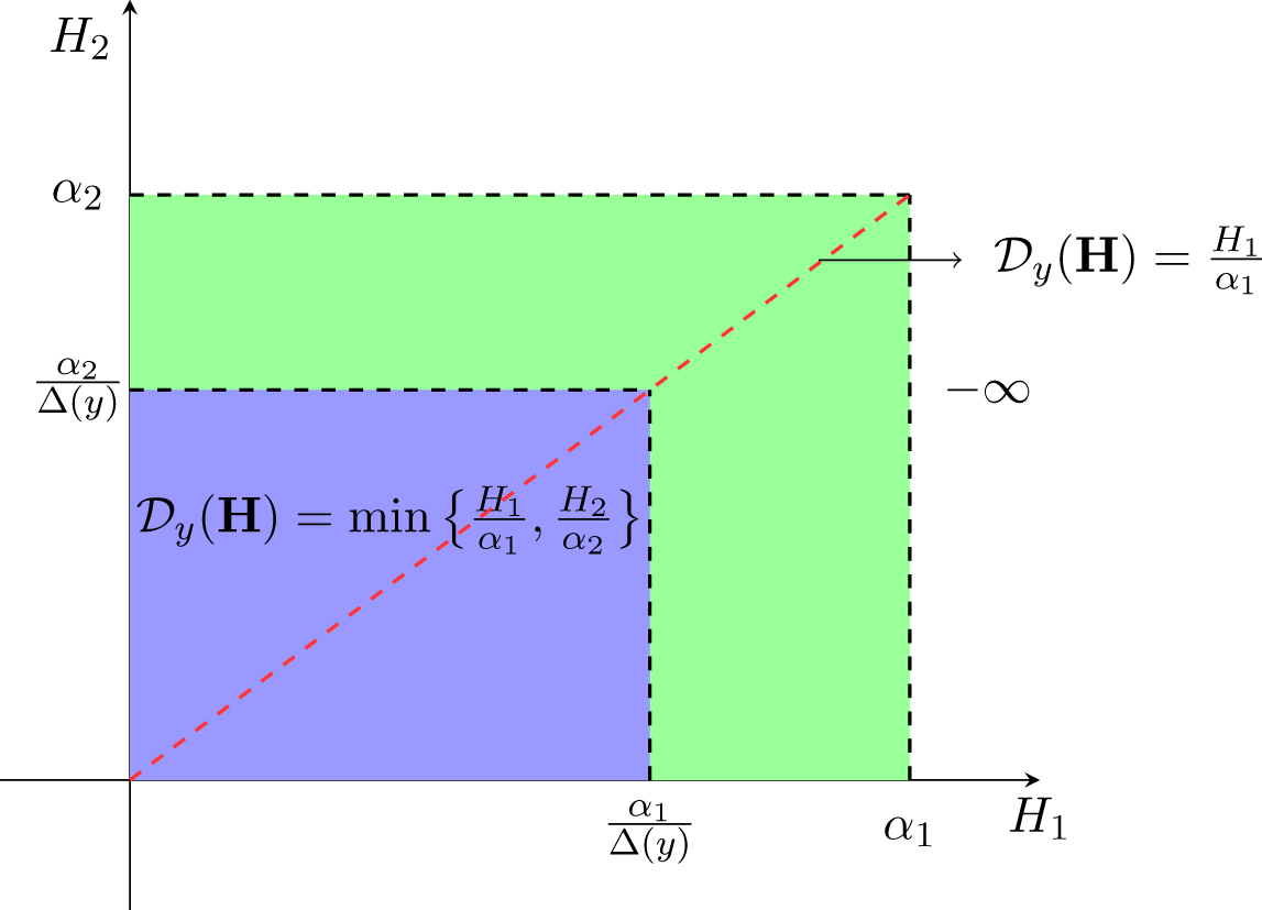
 $\left[0,\frac{\alpha_1}{\Delta(y)}\right]\times \left[0,\frac{\alpha_2}{\Delta(y)}\right]$ (see Figure 1).
The spectrum on the red line is  $\frac{H_1}{{\alpha_1}}$, and the spectrum on the blue rectangle is
 $\min\left\{\frac{H_1}{{\alpha_1}}, \frac{H_2}{{\alpha_2}}\right\}$.

The following theorem will be proven in Section 4.
Theorem 2.3. The bivariate multifractal spectrum of the Lévy function  $L_{\alpha_1}$ and the translated function
 $L_{\alpha_2}^{y}$ satisfies
 \begin{equation*}
\mathcal{D}_{y}(\textbf{H})=
\begin{cases}
\min\left\{\frac{H_1}{\alpha_1}, \frac{H_2}{{\alpha_2}}\right\}, & \quad {\rm if}\ {\textrm{\textbf{H}}} \in K_y,\\
-\infty & \quad {\rm if} \ {\textrm{\textbf{H}}} \notin [\textbf{0}, \boldsymbol{\alpha}].
\end{cases}
\end{equation*}
As corollary, the bivariate multifractal spectrum for almost all translations follows.
Corollary 2.4. For almost every  $y$, the bivariate multifractal spectrum of the Lévy function
 $L_{\alpha_1}$ and the translated function
 $L_{\alpha_2}^{y}$ is
 \begin{equation*}
\mathcal{D}_{y}(\textbf{H})=
\begin{cases}
\min\left\{\frac{H_1}{{\alpha_1}}, \frac{H_2}{{\alpha_2}}\right\}, & \quad {\rm if}\ {\textrm{\textbf{H}}}\in [\textbf{0},\boldsymbol{\alpha}],\\
-\infty & \quad {\rm else}.
\end{cases}
\end{equation*}
Proof. Let
 \begin{equation*}E_{\alpha}=\left\{y:\ \left|y-\frac{k}{b^n}\right| \leqslant \frac{1}{b^{\alpha n}}\ \text{for infinitely many } n\right\},\end{equation*}
and
 \begin{equation*}A_{\eta}=\{y: \Delta (y)=\eta\},\ (\eta\geqslant 1).\end{equation*}
Then
 \begin{equation*}
A_{\eta}=\bigcap\limits_{\alpha\leqslant\eta} E_\alpha - \bigcup \limits_{\alpha \gt \eta} E_\alpha.
\end{equation*}
By a straightforward covering argument, see e.g. [Reference Philipp35, Theorem 2],  $E_1=\mathbb{R}$ and
 $m(E_\alpha)=0$ for any
 $\alpha \gt 1$, where
 $m(\cdot)$ denote the Lebesgue measure. Hence, for almost all
 $y$,
 $\Delta (y)=1$, and
 \begin{equation*}
K_y=[\textbf{0},\boldsymbol{\alpha}].
\end{equation*}
Remark 1. The bivariate multifractal spectrum  $\mathcal{D}_{y}$ in the region
 $K_y$ only depends on the
 $b$-adic approximation properties and is given by Theorem 2.3 for any parameter
 $y\in \mathbb{R}$. But the spectrum in the region
 $ [\textbf{0},\boldsymbol{\alpha}] \setminus K_y$ (the green part in Figure 1), can be different for different values of
 $y$ which share the same
 $b$-adic approximation exponent
 $\Delta (y)$: it actually depends on the explicit expression of the
 $b$-ary expansion (see Subsection 3.2) of
 $y$, as shown by Propositions 2.6 and 2.7. The full determination of the support of the bivariate multifractal spectra for all values of
 $y$ remains to be settled. However, the following result shows that this spectrum can take two values only.
Theorem 2.5. Let  $\textbf{H}\in [\textbf{0},\boldsymbol{\alpha}]{\backslash} K_y$. Then the bivariate multifractal spectrum of the Lévy function
 $L_{\alpha_1}$ and the translated function
 $L_{\alpha_2}^{y}$ is either
 \begin{equation*}
\mathcal{D}_{y}(\textbf{H})=\min\left\{\frac{H_1}{{\alpha_1}}, \frac{H_2}{{\alpha_2}}\right\},
\end{equation*}
or
 \begin{equation*}
\mathcal{D}_{y}(\textbf{H})=-\infty.
\end{equation*}
The proof of Theorem 2.5 will be given in Section 5.
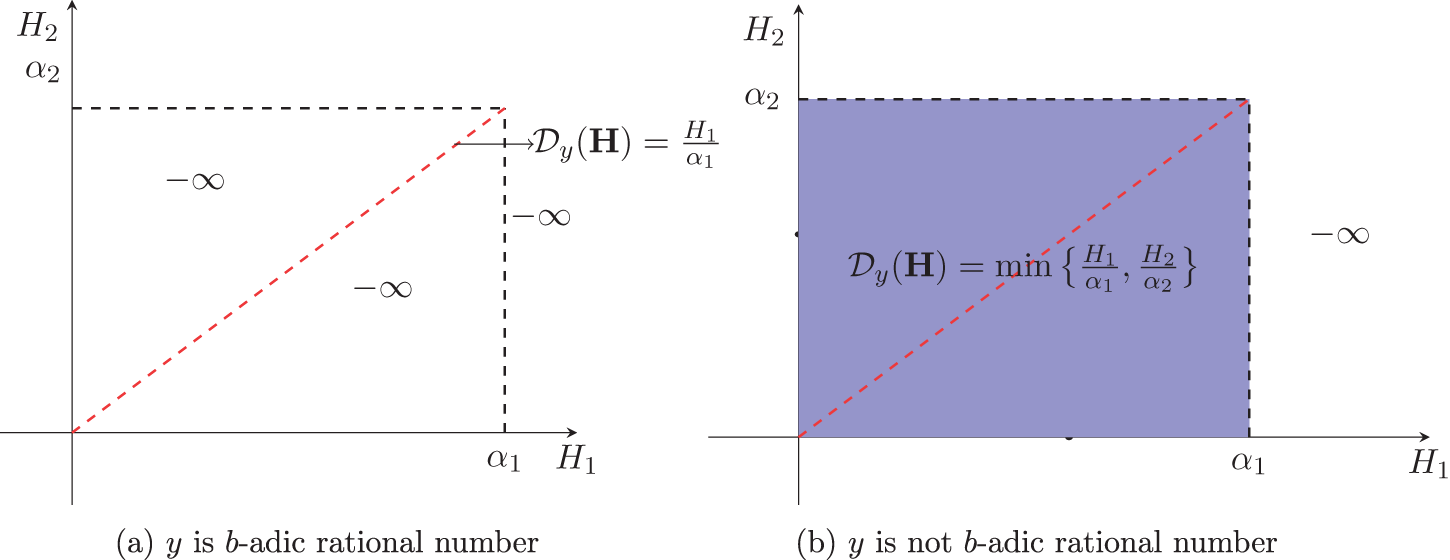
Remark 2. For any rational number, if  $y$ is a
 $b$-adic rational number, then the bivariate multifractal spectrum of the Lévy functions
 $L_{\alpha_1}$ and
 $L_{\alpha_2}^{y}$ takes the following values on the diagonal
 $\frac{H_1}{{\alpha_1}} = \frac{H_2}{{\alpha_2}}$, should be
 \begin{equation*}
\begin{aligned}
\mathcal{D}_{y}(\textbf{H})=
\begin{cases}
\frac{H_1}{{\alpha_1}}, & \quad {\rm if}\ H_2 = \frac{{\alpha_2}}{{\alpha_1}}H_1,\ {\rm and}\ H_1\in [0,\alpha_1],\\
-\infty & \quad {\rm else}.
\end{cases}
\end{aligned}
\end{equation*}
see Figure 2a.
Bivariate multifractal spectrum  $\mathcal{D}_{y}$ of Lévy functions when
 $y$ is a rational number. (a)
 $y$ is
 $b$-adic rational number. (b)
 $y$ is not
 $b$-adic rational number.

If  $y$ is not a
 $b$-adic rational number, then the bivariate multifractal spectrum of the Lévy functions
 $L_{\alpha_1}$ and
 $L_{\alpha_2}^{y}$ is
 \begin{equation*}
\mathcal{D}_{y}(\textbf{H})=
\begin{cases}
\min\left\{\frac{H_1}{{\alpha_1}}, \frac{H_2}{{\alpha_2}}\right\}, & \quad {\rm if}\ \textbf{H}\in [\textbf{0},\boldsymbol{\alpha}],\\
-\infty & \quad {\rm else},
\end{cases}
\end{equation*}
see Figure 2b.
In fact, on one hand, if  $y$ is
 $b$-adic rational, then the two Lévy functions differ only by a finite sum of terms
 $\frac{\{b^iy\}}{b^{\alpha i}}$ and the result is immediate. On the other hand, if
 $y$ is not
 $b$-adic rational, then
 $\Delta(y)=1$. Consequently, the result follows directly as a corollary of Theorem 2.3.
To end this section, we state the following propositions which show that the bivariate multifractal spectrum depends on the explicit expression of the  $b$-ary expansion of
 $y$ when
 $\textbf{H}$ satisfies
 $\min\left\{\frac{{\alpha_1}}{H_1} ,\frac{{\alpha_2}}{H_2}\right\} \lt \Delta (y)$ (the green part in Figure 1).
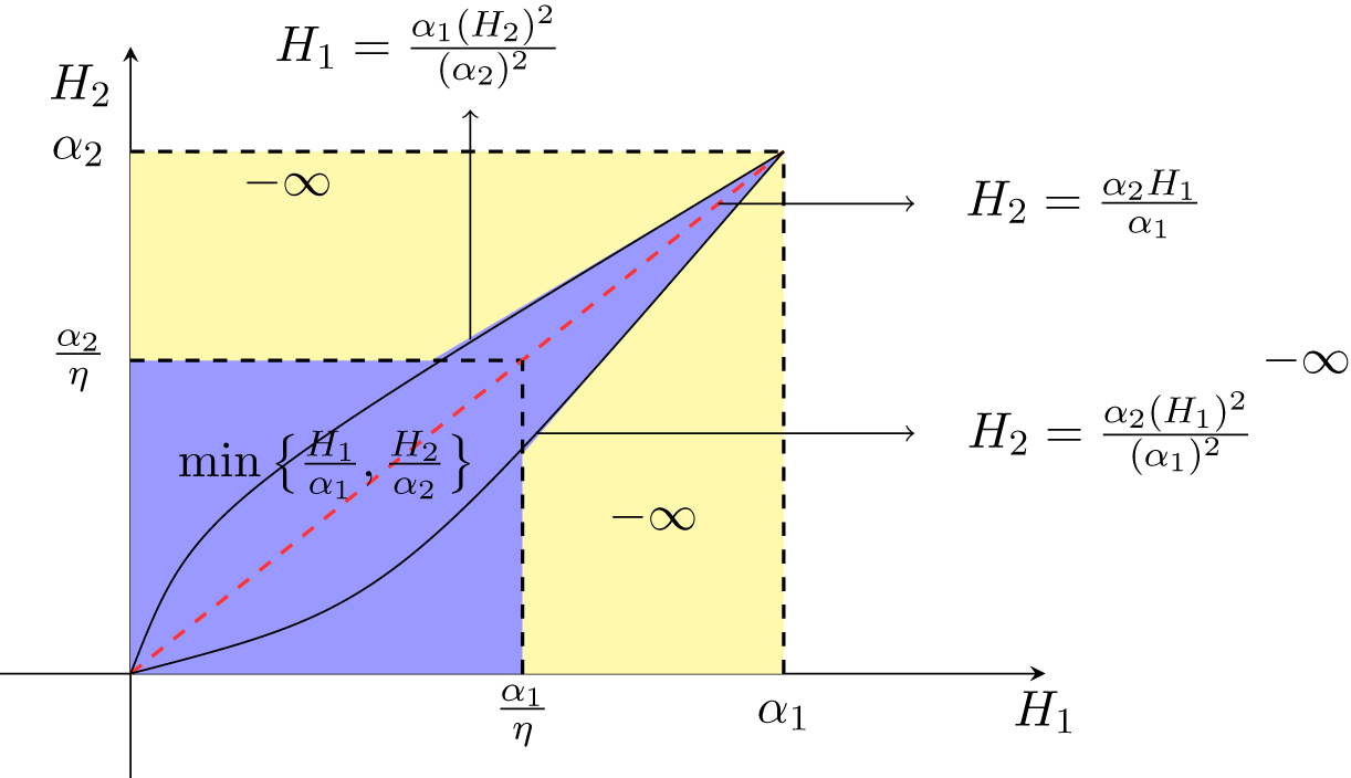
Proposition 2.6. Let  $\eta \gt 1$. Let
 $\{l_i\}$ be an increasing sequence of integers defined by
 \begin{equation*}
l_{i+1}=\lfloor l_i\eta \rfloor,\ \forall i\geqslant 1.
\end{equation*}
and  $\nu_k=0^{\lfloor l_i\eta\rfloor-l_i-1}1$, where
 $l_1$ is a sufficiently large integer. If the
 $b$-ary expansion of
 $y$ is
 $\nu_1\nu_2\nu_3\cdots$ (see Figure 3), then
 $\Delta (y)=\eta$, and the bivariate multifractal spectrum of the Lévy functions
 $L_{\alpha_1}$ and
 $L_{\alpha_2}^{y}$ is
 \begin{equation*}
\mathcal{D}_{y}(\textbf{H})=
\begin{cases}
\frac{H_1}{{\alpha_1}}, & \ {\rm for} \quad \big(H_1, \frac{{\alpha_2}}{{\alpha_1}} H_1\big) \ {\rm with} \ H_1\in [0, {\alpha_1} ],\\
\min\left\{\frac{H_1}{{\alpha_1}}, \frac{H_2}{{\alpha_2}}\right\}, & \ {\rm if}\ \textbf{H} \in \Big{[}0,\frac{{\alpha_1}}{\eta}\Big{]}\times \Big{[}0,\frac{{\alpha_2}}{\eta}\Big{]}
\\ &\ {\rm or}\ H_1 \in \Big{[}\frac{\alpha_1(H_2)^2}{(\alpha_2)^2},\frac{{\alpha_1H_2}}{{\alpha_2}}\Big{]} \ {\rm with} \ H_2\in \left[\frac{\alpha_2}{\eta}, {\alpha_2} \right]
,\\ &\ {\rm or}\ H_2 \in \Big{[}\frac{\alpha_2(H_1)^2}{(\alpha_1)^2},\frac{{\alpha_2H_1}}{{\alpha_1}}\Big{]} \ {\rm with} \ H_1\in \left[\frac{\alpha_1}{\eta}, {\alpha_1} \right]\\
-\infty & \ {\rm else}.
\end{cases}
\end{equation*}
The  $b$-ary expansion of
 $y$.

See Figure 4, for illustration.
Bivariate multifractal spectrum of Propositions 2.6.

Proposition 2.7. Let  $\{l_i\}$ be an increasing sequence of integers satisfying
 \begin{equation*}
\begin{aligned}
\lim\limits_{i\to+\infty}\frac{l_{i-1}}{l_i}=0.
\end{aligned}
\end{equation*}
Let
 \begin{equation*}
\nu_i=
\begin{cases}
0^{\lfloor l_i\eta\rfloor-l_i}1(01)^{\lfloor(l_{i+1}-\lfloor l_i\eta\rfloor-1)/2\rfloor} & \text{if $(l_{i+1}-\lfloor l_i\eta\rfloor-1)/2$ is even,}\\
0^{\lfloor l_i\eta\rfloor-l_i}1(01)^{\lfloor(l_{i+1}-\lfloor l_i\eta\rfloor-1)/2\rfloor}1 & \text{if $(l_{i+1}-\lfloor l_i\eta\rfloor-1)/2$ is odd}.
\end{cases}
\end{equation*}
If the  $b$-ary expansion of
 $y$ is
 $\nu_1\nu_2\nu_3\cdots$ (see Figure 5), then the bivariate multifractal spectrum of the Lévy functions
 $L_{\alpha_1}$ and
 $L_{\alpha_2}^{y}$ is
 \begin{equation*}
\mathcal{D}_{y}(\textbf{H})=
\begin{cases}
\min\left\{\frac{H_1}{{\alpha_1}}, \frac{H_2}{{\alpha_2}}\right\}, & \quad {\rm if}\ \textbf{H}\in [\mathbf{0},\boldsymbol{\alpha}],\\
-\infty & \quad {\rm else}.
\end{cases}
\end{equation*}
The  $b$-ary expansion of
 $y$ (here we take the example of
 $(l_{i+1}-\lfloor l_i\eta\rfloor-1)/2$ being an even number).

Propositions 2.6 and 2.7 will be proven in Section 6.
3. Preliminaries
3.1. Hölder exponent of Lévy functions and Diophantine approximation
Recall that the notions related to the approximation exponent have been introduced in Definition 2.2. It follows from (2.3) that
 \begin{equation}
\Delta (x-y)=\sup\left\{\alpha\geqslant1: \lVert b^n(x-y) \rVert \leqslant \frac{1}{b^{n(\alpha-1)}}{\rm\ for\ infinitely \ many}\ n\right\}.
\end{equation}
Let  $h(x)$ and
 $h^{y}(x)$ denote the Hölder exponents of
 $L_\alpha$ and
 $L_\alpha^y$ at
 $x$, respectively. For any
 $H \gt 0$, define the level sets
 \begin{equation*}
E(H) := \{x \in \mathbb{R} : h(x) = H \}, \quad
E^{y}(H) := \{x \in \mathbb{R} : h^{y}(x) = H \},
\end{equation*}
and their Hausdorff dimensions
 \begin{equation*}
\mathcal{D}(H) := \dim_H\big(E(H)\big), \quad
\mathcal{D}^{y}(H) := \dim_H\big(E^{y}(H)\big).
\end{equation*}
The following proposition gives the Hölder exponent of the Lévy function  $L_{\alpha}$.
Proposition 3.1. [[Reference Jaffard14], Proposition 4] The Hölder exponent of  $L_{\alpha}$ is
 \begin{equation*}
h(x)= \frac{{\alpha}}{\Delta (x)}.
\end{equation*}
On the other hand, observe that
 \begin{equation}
h^y(x)=h(x-y).
\end{equation}
So, by Proposition 3.1,
 \begin{equation}
h^y(x) =\frac{{\alpha}}{\Delta (x-y)}.
\end{equation}
Remark 3. By Proposition 3.1 and (3.3), for any  $\textbf{H}\in [\mathbf{0}, \boldsymbol{\alpha}]$,
 \begin{equation}
\begin{aligned}
E_{y}(\textbf{H})&=\left\{x \in \mathbb{R}:\Delta (x) = \frac{{\alpha_1}}{H_1}\right\}\cap\left\{x \in \mathbb{R}: \Delta(x-y)=\frac{{\alpha_2}}{H_2}\right\}\\
&=E_{1}(H_1)\cap E_{2}(H_2).
\end{aligned}
\end{equation}
The main issue of the paper is to determine the Hausdorff dimension of the level set  $E_{y}(\textbf{H})$, which is by (3.4) an intersection of two fractal sets. For each of the two sets in the intersection, its Hausdorff dimension is already known. The univariate multifractal spectrum
 $\mathcal{D}$ (i.e. the Hausdorff dimension of the first fractal set in the intersection (3.4), applied with
 $\alpha=\alpha_1$) was obtained by S. Jaffard [Reference Jaffard14].
Proposition 3.2. ([Reference Jaffard14], Proposition 4)
The multifractal spectrum  $\mathcal{D}:H\mapsto \dim_H\left(E(H)\right)$ of the Lévy function
 $L_{\alpha}$ is given by
 \begin{equation*}
\begin{aligned}
\mathcal{D}(H)=
\left\{
\begin{array}{ll}
\frac{H}{{\alpha}},&\quad {\rm if}\ H \in [0,{\alpha}],\\
-\infty,&\quad{\rm else}.
\end{array}
\right.
\end{aligned}
\end{equation*}
Noting that by (3.2), for any given  $y\in \mathbb{R}$ and
 $H \gt 0$, we have
 $E^y(H)=E(H)+ y $, it follows directly that the univariate multifractal spectrum
 $\mathcal{D}^y$ (i.e. the Hausdorff dimension of the second fractal set in the intersection (3.4) under
 $\alpha=\alpha_2$), is
 \begin{equation*}
\begin{aligned}
\mathcal{D}^y(H)=
\left\{
\begin{array}{ll}
\frac{H}{{\alpha}},&\quad {\rm if}\ H \in [0,{\alpha}],\\
-\infty&\quad{\rm else}.
\end{array}
\right.
\end{aligned}
\end{equation*}
The following Billingsley’s lemma is useful for calculating the Hausdorff dimension. Let  $\mu$ be a finite Borel measure on
 $[0,1]$. For
 $x\in [0,1]$, let
 $I_n(x)$ be the
 $n$-th generation, half-open
 $b$-adic interval of the form
 $[{\frac{j-1}{b^n}}, \frac{j}{b^n})$ containing
 $x$. The lower local pointwise dimension
 $\underline{d}_{\mu}(x)$ at
 $x$ is defined by
 \begin{equation}
\underline{d}_{\mu}(x)=\mathop{\liminf}\limits_{n\rightarrow \infty}\frac{\log\mu\big(I_n(x)\big)}{\log |I_n(x)|}.
\end{equation}
Lemma 3.3. (C. J. Bishop and Y. Peres,2016 Billingsley’s lemma, [Reference Bishop and Peres6, p.17])
Let  $E$ be a Borel subset of
 $[0,1]$ and
 $\mu$ a finite Borel measure on
 $[0,1]$. (1) If
 $\underline{d}_{\mu}(x) \geqslant s$ for all
 $\mu$-almost all
 $x \in E$, and
 $\mu(E) \gt 0$, then
 $\dim_H(E)\geqslant s$. (2) If
 $\underline{d}_{\mu}(x) \leqslant s$ for all
 $x \in E$, then
 $\dim_H(E)\leqslant s$.
3.2. Symbolic space and  $b$- ary expansion

Since Lévy functions are 1-periodic, they can be considered as functions defined on the interval  $[0,1)$. The level sets
 $E_{y}(\textbf{H})$ will also be considered as their intersection with
 $[0,1)$.
Denote  $\mathcal{A}:=\{0,1,\cdots,b-1\}$. Denote by
 $\mathcal{A}^n$ the set of all words of length
 $n$ over
 $\mathcal{A}$, and let
 $\mathcal{A}^*=\bigcup\limits_{n=1}^\infty\mathcal{A}^n$ be the set of all finite words over
 $\mathcal{A}$. Every number
 $x$ in
 $[0,1)$ admits a
 $b$-ary expansion
 \begin{equation*}
x=\sum\limits_{i=1}^{\infty} \frac{\varepsilon_i}{b^i},\quad \text{with} \ \varepsilon_i\ \in \mathcal{A}.
\end{equation*}
Then a number  $x \in [0,1)$ is associated with an infinite word
 $\varepsilon=\varepsilon_1\varepsilon_2\cdots$ which is also referred to as the
 $b$-ary expansion of
 $x$. In fact, there is a projection map
 $\Pi:\mathcal{A}^{\mathbb{N}}\longmapsto[0,1)$ defined by
 \begin{equation*}
\Pi(\varepsilon)=\sum\limits_{i=1}^{\infty} \frac{\varepsilon_i}{b^i},\quad \forall \varepsilon=\varepsilon_1\varepsilon_2\cdots\in\mathcal{A}^{\mathbb{N}}.
\end{equation*}
The map  $\Pi$ is one-to-one except for the
 $b$-adic rationals (where it is two-to-one).
If  $x$ is a
 $b$-adic rational number, denoted by
 $x=\frac{k}{b^m}$,
 $(\text{where}\ \gcd(k,b)=1)$, then the
 $b$-ary expansion
 $\varepsilon_1\varepsilon_2\cdots$ of
 $\frac{k}{b^m}$ satisfies one of the following two conditions,
•
$\varepsilon_m= a,\ \varepsilon_k=0,\ \forall k \gt m;$•
$\varepsilon_m = a-1,\ \varepsilon_k=b-1,\ \forall k \gt m, $


where  $a\in \mathcal{A}\backslash\{0\}$. In this paper, the
 $b$-ary expansion of the
 $b$-adic rational number
 $\frac{k}{b^m}$ is the one which satisfies
 $\varepsilon_m=a$,
 $\varepsilon_k=0$ for all
 $k \gt m$.
To study the approximation properties in (2.3) and (3.1), it is more convenient to work on the space  $\Sigma:=\mathcal{A}^{\mathbb{N}}$ of infinite words. The space
 $\Sigma$ is naturally equipped with a metric defined by
 \begin{equation*}
\forall \varepsilon, \varepsilon' \in \Sigma, \ d(\varepsilon,\varepsilon')=b^{-\min\{n\geqslant 0:\ \varepsilon_{n+1}\neq\varepsilon'_{n+1}\}}.
\end{equation*}
Define the left shift  $\sigma$ on
 $\Sigma$ by
 \begin{equation*}
\sigma: \varepsilon_1\varepsilon_2\cdots\longmapsto\varepsilon_2\varepsilon_3\cdots.
\end{equation*}
If the infinite word associated with  $x$ is
 $\varepsilon$, then for any
 $n$, the infinite word associated with
 $b^nx$ is
 $\sigma^n(\varepsilon)$. For any
 $a \in \mathcal{A}$,
 $k \in \mathbb{N}$, denote
 $a^k=\underbrace{aa\cdots a}_{k}$ and
 $a^\infty=aa\cdots$. Then,
 \begin{equation*}
\frac{1}{b}d\big(\sigma^{n}(\varepsilon),\varepsilon^*\big) \leqslant \|b^nx\|\leqslant d\big(\sigma^{n}(\varepsilon),\widetilde{\varepsilon}\big),
\end{equation*}
where  $\varepsilon^*,\ \widetilde{\varepsilon}=0^\infty $ or
 $(b-1)^\infty$. As a consequence, if
 $\sigma^n(\varepsilon)$ is followed by a word
 $\varepsilon_{n+1}\varepsilon_{n+2}\cdots$, where
 \begin{equation*}
\begin{aligned}
&\varepsilon_{n+1}\varepsilon_{n+2}\cdots\varepsilon_{n+m}=0^{m},\\
&\varepsilon_{n+m+1}\neq 0,
\end{aligned}
\end{equation*}
or
 \begin{equation*}
\begin{aligned}
&\varepsilon_{n+1}\varepsilon_{n+2}\cdots\varepsilon_{n+m}=(b-1)^{m},\\
&\varepsilon_{n+m+1}\neq b-1,
\end{aligned}
\end{equation*}
then
 \begin{equation}
\frac{1}{b^{m+1}}\leqslant \lVert b^{n}x\rVert \leqslant \frac{1}{b^{m}}.
\end{equation}
Let  $\theta=\theta_1\theta_2\cdots$ be the
 $b$-ary expansion of
 $y$. If
 \begin{equation*}
\begin{aligned}
&\varepsilon_{n+1}\varepsilon_{n+2}\cdots\varepsilon_{n+m}=\theta_{n+1}\theta_{n+2}\cdots\theta_{n+m},\\
&\varepsilon_{n+m+1}\neq \theta_{n+m+1},
\end{aligned}
\end{equation*}
then
 \begin{equation}
\frac{1}{b^{m+1}}=\frac{1}{b}d\big(\sigma^{n}(\varepsilon),\sigma^{n}(\theta)\big) \leqslant \lVert b^{n}(x-y)\rVert \leqslant d\big(\sigma^{n}(\varepsilon),\sigma^{n}(\theta)\big)=\frac{1}{b^{m}}.
\end{equation}
For  $\varepsilon_1\varepsilon_2\cdots\varepsilon_n \in \mathcal{A}^n$, denote by
 $I_n(\varepsilon_1\varepsilon_2\cdots\varepsilon_n)$ the cylinder of order
 $n$ composed of real numbers in
 $[0,1)$ whose
 $b$-ary expansions start with
 $\varepsilon_1\varepsilon_2\cdots\varepsilon_n$. Then,
 $I_n(\varepsilon_1\varepsilon_2\cdots\varepsilon_n)$ is an interval of length
 $b^{-n}$.
4. Multivariate multifractal spectra of Lévy functions
In this section, we prove Theorem 2.3 which gives the multivariate multifractal spectra of a Lévy function and its translations.
The upper bound of the spectrum in Theorem 2.3 follows from straightforward observations. The main effort in the proof lies in establishing the lower bound.
The strategy for proving the lower bound for  $\mathbf{H}\in\widetilde{K}_y$ proceeds as follows. We begin by constructing a Cantor-type subset of the level set
 $ E_{y}(\textbf{H}) $ for any
 $ \textbf{H} \in \widetilde{K}_y$ (Subsections 4.1 and 4.2). Then, we will define a measure on the Cantor-type subset and estimate its lower local dimensions (Subsection 4.3). Finally, we obtain the lower bound of the Hausdorff dimension of the Cantor-type subset using Billingsley’s lemma (Subsection 4.4). Such lower bound is nothing but the wanted lower bound of the spectrum. Furthermore, the spectra for
 $\textbf{H}\in {\rm DL}$ and
 $\textbf{H}\notin [\textbf{0}, \boldsymbol{\alpha}]$ are obtained as well (Subsection 4.4).
4.1. Construction of Cantor-type subsets
In this subsection, given data  $y\in [0,1]$,
 $\alpha_1 \gt 0, \alpha_2 \gt 0$,
 $\textbf{H}\in \widetilde{K}_y$, we construct a Cantor-type subset of
 $ E_{y}(\textbf{H})$.
Suppose  $y \in[0,1]$ has
 $b$-ary expansion
 $\theta=\theta_1\theta_2\cdots$. Let
 $\{n_k\}_{k\geqslant0}$ be a sequence of integers satisfying
 \begin{equation}
\begin{aligned}
\frac{k\cdot n_{k-1}}{n_{k}}\rightarrow 0,\ (k\rightarrow \infty).
\end{aligned}
\end{equation}
For any  $k \geqslant 0$, let
 \begin{equation}
\begin{aligned}
&m_{k} = \left\lfloor n_{k}\left(\frac{{\alpha_1}}{H_1}-1\right)\right\rfloor,\\
&m'_{k} = \left\lfloor n_{k}\left(\frac{{\alpha_2}}{H_2}-1\right)\right\rfloor,
\end{aligned}
\end{equation}
and
 \begin{equation*}
m^*_{k}=\min\{m_{k},m'_{k}\}.
\end{equation*}
If  $n_0\leqslant m^*_{0}$, then define
 \begin{equation*}
\begin{aligned}
\mathcal{W}_{0}=\left\{ \varepsilon_{1}\varepsilon_{2}\cdots\varepsilon_{n_{0}}\in\mathcal{A}^*:\ \varepsilon_{n_{0}-1}=0\ \text{and}\ \varepsilon_{n_{0}}=1 \right\}.
\end{aligned}
\end{equation*}
If  $n_0 \gt m^*_{0}$, then let
 \begin{equation}
r_{0}=\left\lfloor \frac{n_{0}-2}{m^*_{0}}\right\rfloor,
\end{equation}
and define
 \begin{equation*}
\begin{aligned}
\mathcal{W}_{0}=\Big\{
\varepsilon_{1}\varepsilon_{2}\cdots\varepsilon_{n_{0}}\in\mathcal{A}^*:\ &\varepsilon_j=0 \ \text{for}\ j= n_{0}-1,\ \text{and}\ j=tm^*_{0}-1,\ 1\leqslant t \leqslant r_{0};\\ &\varepsilon_j=1\ \text{for}\ j= n_{0}, \ \text{and}\ j=tm^*_{0}\ 1\leqslant t \leqslant r_{0} \Big\}.
\end{aligned}
\end{equation*}
Note that  $2$ is subtracted in (4.3) to avoid the possibility of doubly defining the values of
 $\varepsilon_{n_0-1}$ and
 $\varepsilon_{n_0}$ in
 $\mathcal{W}_{0}$.
By (4.1) and (4.2), without loss of generality, assume that
 \begin{equation}
\begin{aligned}
n_{2k+1}-n_{2k}-m_{2k}-8 \gt 0,
\end{aligned}
\end{equation}
 \begin{equation}
\begin{aligned}
n_{2k+2}-n_{2k+1}-m'_{2k+1}-9 \gt 0.
\end{aligned}
\end{equation}
Then, let
 \begin{equation*}
\ r_{2k}=\left\lfloor \frac{n_{2k+1}-n_{2k}-m_{2k}-8}{m^*_{2k}}\right\rfloor,
\end{equation*}
 \begin{equation*}
r_{2k+1}=\left\lfloor \frac{n_{2k+2}-n_{2k+1}-m'_{2k+1}-9}{m^*_{2k+1}}\right\rfloor.
\end{equation*}
For any  $k\geqslant 0$, define
 \begin{equation*}
\begin{aligned}
\mathcal{W}_{2k+1}=\Big\{
\varepsilon_{1}\varepsilon_{2}\cdots\varepsilon_{n_{2k+1}-n_{2k}}\in\mathcal{A}^*:\ &\varepsilon_j=0 \ \text{for}\ 1\leqslant j \leqslant m_{2k},\ j= n_{2k+1}-n_{2k}-2,\\ &\ \ \ \ \ \ \ \ \ \text{and}\ j=m_{2k}+tm^*_{2k},\ 1\leqslant t \leqslant r_{2k};\\ &\varepsilon_j = 1\ \text{for}\ j=m_{2k}+tm^*_{2k}+1,\ 0\leqslant t \leqslant r_{2k},\\ &\ \ \ \ \ \ \ \ \ \text{and}\ j= n_{2k+1}-n_{2k}-1;
\\ &\varepsilon_j\neq\theta_{n_{2k}+j}\ \text{for}\ j=m_{2k}+tm^*_{2k}+2,
\\ &\ \ \ \ \ \ \ \ \ \ \quad 0\leqslant t\leqslant r_{2k},\ \text{and}\ j= n_{2k+1}-n_{2k} \Big\},
\end{aligned}
\end{equation*}
and
 \begin{equation*}
\begin{aligned}
\mathcal{W}_{2k+2}=\Big\{
\varepsilon_{1}\varepsilon_{2}\cdots\varepsilon_{n_{2k+2}-n_{2k+1}}\in\mathcal{A}^*: \ &\varepsilon_j=\theta_{n_{2k+1}+j} \ \text{for}\ 1\leqslant j \leqslant m'_{2k+1};\\ & \varepsilon_j\neq\theta_{n_{2k+1}+j} \ \text{for}\ j=m'_{2k+1}+tm^*_{2k+1},\\ &\ 0\leqslant t \leqslant r_{2k+1},\ \text{and}\ j= n_{2k+2}-n_{2k+1}-2;
\\ &\varepsilon_j=0 \ \text{for}\ j=m'_{2k+1}+tm^*_{2k+1}+1,\\ &\ 0\leqslant t\leqslant r_{2k+1},\ \text{and}\ j= n_{2k+2}-n_{2k+1}-1;
\\ &\varepsilon_j = 1\ \text{for}\ j=m'_{2k+1}+tm^*_{2k+1}+2,\\ &\ \ \ 0\leqslant t\leqslant r_{2k+1},\ \text{and}\ j= n_{2k+2}-n_{2k+1} \Big\}.
\end{aligned}
\end{equation*}
For better illustration, the notation  $\varepsilon_i = \overline\theta_i$ is used whenever
 $\varepsilon_i \neq \theta_i$. Hence, the words in
 $\mathcal{W}_{2k+1}$ begin with
 $0^{m_{2k}}1\overline\theta_{n_{2k}+m_{2k}+2}$, contain a subword
 $01\overline\theta_{n_{2k}+m_{2k}+tm^*_{2k}+2}$ at the positions
 $m_{2k}+tm^*_{2k}$, and end with
 $01\overline\theta_{n_{2k+1}}$. Similarly, the words in
 $\mathcal{W}_{2k+2}$ begin with
 $\theta_{n_{2k+1}+1}\cdots\theta_{n_{2k+1}+m'_{2k+1}}\overline\theta_{n_{2k+1}+m'_{2k+1}+1}01$, contain a subword
 $\overline\theta_{n_{2k+1}+m'_{2k+1}+tm^*_{2k+1}}01$ at the positions
 $m_{2k+1}+tm^*_{2k+1}$, and end with
 $\overline\theta_{n_{2k+2}-2}01$. See Figures 6 and 7 for illustrations.
The construction of  $\mathcal{W}_{2k+1}$.

The construction of  $\mathcal{W}_{2k+2}$.

Notice that  $8$ is subtracted in (4.4), to well define
 $\mathcal{W}_{2k+1}$. Precisely, the following
 $8$ values should be defined only once:
 \begin{equation*}
\begin{aligned}
&\varepsilon_{m_{2k}+1}= 1,
\\ &\varepsilon_{m_{2k}+2}\neq\theta_{m_{2k}+2},
\\ &\varepsilon_{m_{2k}+r_{2k}m^*_{2k}}=0,
\\ &\varepsilon_{m_{2k}+r_{2k}m^*_{2k}+1}=1,
\\ &\varepsilon_{m_{2k}+r_{2k}m^*_{2k}+2}\neq\theta_{m_{2k}+r_{2k}m^*_{2k}+2},
\\ &\varepsilon_{n_{2k+1}-n_{2k}-2}=0,
\\ &\varepsilon_{n_{2k+1}-n_{2k}-1}=1,
\\ &\varepsilon_{n_{2k+1}-n_{2k}}\neq\theta_{n_{2k+1}-n_{2k}}.
\end{aligned}
\end{equation*}
Similarly, we subtract  $9$ in (4.5).
Take
 \begin{equation*}
\begin{aligned}
\mathcal{U}_k=\{w_0w_1\cdots w_k:w_j\in \mathcal{W}_{j},\ 0\leqslant j\leqslant k\}.
\end{aligned}
\end{equation*}
Our Cantor-type subset is defined as
 \begin{equation}
\begin{aligned}
E&:=\mathop{\bigcap}\limits_{k=0}^{\infty}
\mathop\bigcup_{
u \in \mathcal{U}_{k}}
I_{n_{k+1}}(u).
\end{aligned}
\end{equation}
4.2. Subsets of
$E_{y}(\textbf{H})$

In this subsection, we will prove that  $E$ is a subset of
 $E_{y}(\textbf{H})$. To this end, for any
 $x \in E$, we estimate
 $\lVert b^{n}x \rVert$ and
 $\lVert b^{n}(x-y) \rVert$, respectively.
Note that for  $x\in E$ with
 $\varepsilon=\varepsilon_{1}\varepsilon_{2}\varepsilon_{3}\cdots$ being its
 $b$-ary expansion, it holds that
 \begin{equation*}
\varepsilon=w_0w_1\cdots
\end{equation*}
with  $w_j\in \mathcal{W}_{j}$ for all
 $j\geqslant 0$.
• The estimation for
$\lVert b^{n}x \rVert$.– If
$n=n_{2k}\ (k\geqslant 0),$ then by the definition of
$\mathcal{W}_{2k+1}$,
$\varepsilon_{n_{2k}}$ is followed by
$0^{m_{2k}}1$. Hence, according to (3.6), it follows that,
(4.7)\begin{equation}
\frac{1}{b^{n_{2k}\big(\frac{{\alpha_1}}{H_1}-1\big)+1}} \leqslant \frac{1}{b^{m_{2k}+1}}\leqslant \lVert b^{n_{2k}}x \rVert \leqslant \frac{1}{b^{m_{2k}}}\leqslant \frac{1}{b^{n_{2k}\big(\frac{{\alpha_1}}{H_1}-1\big)-1}}.
\end{equation}By (2.3), it immediately follows that
(4.8)\begin{equation}
\Delta(x)\geqslant \frac{{\alpha_1}}{H_1}.
\end{equation}– Let
$n\in [n_{2k},n_{2k+1}]\ (k\geqslant 0)$. By the definition of
$\mathcal{W}_{2k+1}$,
$\varepsilon_n$ cannot be followed by a word of
$0$’s or a word of
$(b-1)$’s of length larger than
$m_{2k}$. According to (3.6),
\begin{equation*}
\begin{aligned}
&\lVert b^{n}x \rVert \geqslant \frac{1}{b^{m_{2k}}} \geqslant
\frac{1}{b^{n_{2k}\big(\frac{{\alpha_1}}{H_1}-1\big)}} \gt \frac{1}{b^{n\big(\frac{{\alpha_1}}{H_1}-1\big)}}.
\end{aligned}
\end{equation*}Then,
(4.9)\begin{equation}
\begin{aligned}
\Delta(x) \leqslant \frac{{\alpha_1}}{H_1}.
\end{aligned}
\end{equation}– Let
$n\in [n_{2k+1},n_{2k+2}]\ (k\geqslant 0)$. Note that
$ \textbf{H} \in \widetilde{K}_y$. Hence,
$H_1\leqslant \frac{\alpha_1}{\Delta(y)}$. That is,
\begin{equation*}\Delta(y)\leqslant \frac{\alpha_1}{H_1}.\end{equation*}Thus, the prefix of the words in
$\mathcal{W}_{2k+2}$ cannot contain a word of
$0$’s or a word of
$(b-1)$’s of length larger than
$m_{2k+1}$. Then, by the definition of
$\mathcal{W}_{2k+2}$,
$\varepsilon_n$ cannot be followed by a word of
$0$’s or a word of
$(b-1)$’s of length larger than
$m_{2k+1}$. Moreover, by (3.6),
\begin{equation*}
\begin{aligned}
&\lVert b^{n}x \rVert \geqslant \frac{1}{b^{m_{2k+1}}} \geqslant
\frac{1}{b^{n_{2k+1}\big(\frac{{\alpha_1}}{H_1}-1\big)}} \gt \frac{1}{b^{n\big(\frac{{\alpha_1}}{H_1}-1\big)}}.
\end{aligned}
\end{equation*}Thus,
(4.10)\begin{equation}
\begin{aligned}
\Delta(x) \leqslant \frac{{\alpha_1}}{H_1}.
\end{aligned}
\end{equation}
Combining (4.8) (4.9) and (4.10) gives
(4.11)\begin{equation}
\begin{aligned}
\Delta(x)= \frac{{\alpha_1}}{H_1}.
\end{aligned}
\end{equation}• The estimation for
$\lVert b^{n}(x-y) \rVert$.– If
$n=n_{2k+1}\ (k\geqslant 0)$, then by the definition of
$\mathcal{W}_{2k+2}$,
(4.12)\begin{equation}
\begin{aligned}
\frac{1}{b^{n_{2k+1}\big(\frac{{\alpha_2}}{H_2}-1\big)+1}} \leqslant \frac{1}{b^{m'_{2k+1}+1}}\leqslant \lVert b^{n_{2k+1}}(x-y) \rVert &\leqslant \frac{1}{b^{m'_{2k+1}}}\\ &\quad \leqslant \frac{1}{b^{n_{2k+1}\big(\frac{{\alpha_2}}{H_2}-1\big)-1}}.
\end{aligned}
\end{equation}Based on (3.1), it follows that
(4.13)\begin{equation}
\Delta(x-y) \geqslant \frac{{\alpha_2}}{H_2}.
\end{equation}– Let
$n\in [n_{2k+1},n_{2k+2}]\ (k\geqslant 0)$. By the definition of
$\mathcal{W}_{2k+1}$,
$\varepsilon_n$ cannot be followed by a word, as a prefix of
$\theta_1\theta_2\cdots$, of length
$m'_{2k+1}$. By (3.7),
\begin{equation*}
\begin{aligned}
&\lVert b^{n}(x-y) \rVert \geqslant \frac{1}{b^{m'_{2k+1}}} \geqslant
\frac{1}{b^{n_{2k+1}\big(\frac{{\alpha_2}}{H_2}-1\big)}} \gt \frac{1}{b^{n\big(\frac{{\alpha_2}}{H_2}-1\big)}}.
\end{aligned}
\end{equation*}It follows that
(4.14)\begin{equation}
\begin{aligned}
\Delta(x-y) \leqslant \frac{{\alpha_2}}{H_2}.
\end{aligned}
\end{equation}– Let
$n\in [n_{2k+2},n_{2k+3}]\ (k\geqslant 0)$. Note that
$ \textbf{H} \in \widetilde{K}_y$. Hence,
$H_2\leqslant \frac{\alpha_2}{\Delta (y)}$. That is,
\begin{equation*}\Delta (y)\leqslant \frac{\alpha_2}{H_2}.\end{equation*}Thus, the prefix of the words in the
$b$-ary expansion of
$y$ cannot contain a word of
$0$’s of length larger than
$m_{2k+2}'$ in
$\theta_{n_{2k+2}-n_{2k+1}}\theta_{n_{2k+2}-n_{2k+1}+1}\cdots\theta_{m_{2k+2}}$. Then by the definition of
$\mathcal{W}_{2k}$,
$\varepsilon_n$ cannot be followed by a word, as a prefix of
$\theta_1\theta_2\cdots$, of length
$m'_{2k+2}$. By (3.7), it holds that
(4.15)\begin{equation}
\begin{aligned}
&\lVert b^{n}(x-y) \rVert \geqslant \frac{1}{b^{m'_{2k+2}}} \geqslant
\frac{1}{b^{n_{2k+2}\big(\frac{{\alpha_2}}{H_2}-1\big)}} \gt \frac{1}{b^{n\big(\frac{{\alpha_2}}{H_2}-1\big)}}.
\end{aligned}
\end{equation}Hence, based on (4.15), it follows that
(4.16)\begin{equation}
\begin{aligned}
\Delta(x-y) \leqslant \frac{{\alpha_2}}{H_2}.
\end{aligned}
\end{equation}
Combining (4.13) (4.14) and (4.16) yields
(4.17)\begin{equation}
\begin{aligned}
\Delta(x-y)= \frac{{\alpha_2}}{H_2}.
\end{aligned}
\end{equation}





Therefore, by (4.11) and (4.17),
 \begin{equation}
E\subset E_{y}(\textbf{H}).
\end{equation}
4.3. A mass distribution and estimation of the lower local pointwise dimensions
In this subsection, we will first give a mass distribution  $\mu$ on the subset
 $E$. Then, we estimate the lower local pointwise dimensions of the measure
 $\mu$.
Let us give a mass distribution  $\mu$ on the Cantor-type set
 $E$. To this end, by Kolmogorov’s extension theorem (see, for example, [Reference Tao37, Theorem 2.4.4]), it suffices to define the mass on each cylinder. Let
 $x \in E$, and let
 $I_n(x)$ be the cylinder of order
 $n$ containing
 $x$. Let
 $\varepsilon= \varepsilon_1\varepsilon_2\varepsilon_3\cdots$ be the
 $b$-ary expansion of
 $x$. Denote by
 $u_n(x)$ the number of ‘free positions’
 $i$ between
 $1$ and
 $n$, at which
 $\varepsilon_i$ can be chosen in
 $\mathcal{A}$ freely, i.e.
 $\varepsilon_i$ is not fixed by the definition of
 $x \in E$. Then we define
 \begin{equation}
\mu\big(I_{n}(x)\big)=b^{-u_{n}(x)}.
\end{equation}
In the following, the lower local pointwise dimension  $\underline{d}_{\mu}(x)$ as defined in (3.5) of
 $\mu$ at a point
 $x\in E$ will be estimated. First, by (4.19), it holds that for any
 $x\in E$,
 \begin{equation*}
\begin{aligned}
\underline{d}_{\mu}(x)= \mathop{\liminf}\limits_{n\rightarrow \infty}\frac{\log\mu(I_{n}(x))}{\log \lvert I_{n}(x)\rvert}
=\mathop{\liminf}\limits_{n\rightarrow \infty}\frac{\log b^{-u_n(x)}}{\log b
^{-n}}
=\mathop{\liminf}\limits_{n\rightarrow \infty}\frac{u_{n}(x)}{{n}}.
\end{aligned}
\end{equation*}
To further estimate  $u_{n}(x)$, we distinguish the following cases.
• If
$n_{2k} \leqslant n\leqslant n_{2k}+m_{2k}+2$, then by the construction of
$\mathcal{W}_{2k+1}$,
\begin{equation*}
u_{n}(x)=u_{n_{2k}+m_{2k}}(x).
\end{equation*}Hence,
\begin{equation*}
\begin{aligned}
\frac{u_{n}(x)}{n}=\frac{u_{n_{2k}+m_{2k}}(x)}{n} \geqslant \frac{u_{n_{2k}+m_{2k}}(x)}{n_{2k}+m_{2k}+2}.
\end{aligned}
\end{equation*}• If
$n_{2k}+m_{2k}+3\leqslant n \lt n_{2k}+m_{2k}+m^*_{2k}$, then by the construction of
$\mathcal{W}_{2k+1}$,
\begin{equation*}
\begin{aligned}
u_{n}(x)=u_{n_{2k}+m_{2k}}(x)+ n - n_{2k}- m_{2k}-2.\\
\end{aligned}
\end{equation*}Note that
$n-n_{2k}- m_{2k}-2 \gt 0$. Combining the fact that
(4.20)\begin{equation}
\frac{x+a}{y+a}\geqslant\frac{x}{y},\quad \forall a \gt 0,\ x\leqslant y,
\end{equation}it follows that
\begin{equation*}
\begin{aligned}
\frac{\log\mu(I_n(x))}{\log \lvert I_n(x)\rvert}=\frac{u_{n}(x)}{n} &=\frac{u_{n_{2k}+m_{2k}}(x)+ n - n_{2k}- m_{2k}-2}{n_{2k}+m_{2k}+2+n-n_{2k}- m_{2k}-2}\\ &\quad \geqslant\frac{u_{n_{2k}+m_{2k}}(x)}{n_{2k}+m_{2k}+2}.
\end{aligned}
\end{equation*}• If
$n_{2k}+m_{2k}+m^*_{2k}\leqslant n \lt n_{2k+1}$, the same discussions as in the above two cases always apply. Hence, for
$n_{2k}\leqslant n \lt n_{2k+1},$ it can be concluded that
(4.21)\begin{equation}
\frac{\log\mu(I_n(x))}{\log \lvert I_n(x)\rvert} \geqslant\frac{u_{n_{2k}+m_{2k}}(x)}{n_{2k}+m_{2k}+2}.
\end{equation}


Note that
 \begin{equation*}
u_{n_{2k}+m_{2k}}(x)=n_{2k}-\sum\limits_{i=0 }^{k-1}\big(m_{2i}+5\big)-\sum\limits_{i=0 }^{k-1} \big(m'_{2i+1}+6\big)-3\sum\limits_{i=0 }^{2k-1}r_i.
\end{equation*}
On the one hand,
 \begin{equation*}
\begin{aligned}
\sum\limits_{i=0 }^{2k-1}r_i =&\sum\limits_{i=0 }^{k-1} \left\lfloor \frac{n_{2k+1}-n_{2k}-m_{2k}-8}{m^*_{2k}}\right\rfloor + \sum\limits_{i=0 }^{k-1} \left\lfloor \frac{n_{2k+2}-n_{2k+1}-m'_{2k+1}-9}{m^*_{2k+1}}\right\rfloor
\\ \leqslant&
\sum\limits_{i=0 }^{2k-1}\frac{n_{i+1}-n_{i}-m^*_{i}}{m^*_{i}}
\\ \leqslant &
\sum\limits_{i=0 }^{2k-1}\frac{n_{i+1}}{n_{i}\cdot\left(\min\left\{\frac{{\alpha_1}}{H_1}, \frac{{\alpha_2}}{H_2}\right\}-1\right)}
\\ \leqslant & 2k\cdot\frac{n_{2k}}{n_{2k-1}\cdot\left(\min\left\{\frac{{\alpha_1}}{H_1}, \frac{{\alpha_2}}{H_2}\right\}-1\right)},
\end{aligned}
\end{equation*}
and by (4.1), it holds that
 \begin{equation*}
\frac{\sum\limits_{i=0 }^{2k-1}3r_i}{n_{2k}} \rightarrow 0,\quad (k\rightarrow \infty).
\end{equation*}
On the other hand,
 \begin{equation*}
\begin{aligned}
\sum\limits_{i=0 }^{k-1}\left(m_{2i}+5\right)+\sum\limits_{i=0 }^{k-1} \left(m'_{2i+1}+6\right)&=\sum\limits_{i=0 }^{k-1}\left(\left\lfloor n_{2i}\left(\frac{{\alpha_1}}{H_1}-1\right)\right\rfloor+5\right)\\ &\quad +\sum\limits_{i=0 }^{k-1}\left (\left\lfloor n_{2i+1}\left(\frac{{\alpha_2}}{H_2}-1\right)\right\rfloor+6\right)
\\ & \leqslant 2k\cdot n_{2k-1}\cdot\left(\max\left\{\frac{{\alpha_1}}{H_1}, \frac{{\alpha_2}}{H_2}\right\}-1\right) + 11k,
\end{aligned}
\end{equation*}
and by (4.1), it follows that
 \begin{equation*}
\frac{\sum\limits_{i=0 }^{k-1}\big(m_{2i}+5\big)+\sum\limits_{i=0 }^{k-1} \big(m'_{2i+1}+6\big)}{n_{2k}} \rightarrow 0,\quad (k\rightarrow \infty).
\end{equation*}
Therefore,
 \begin{equation}
\begin{aligned}
\mathop{\lim}\limits_{k\rightarrow \infty}\frac{u_{n_{2k}+m_{2k}}(x)}{n_{2k}+m_{2k}+2}
=&\mathop{\lim}\limits_{k\rightarrow \infty}\frac{n_{2k}-\sum\limits_{i=0 }^{k-1}\big(m_{2i}+5\big)-\sum\limits_{i=0 }^{k-1} \big(m'_{2i+1}+6\big)-3\sum\limits_{i=0 }^{2k-1}r_i}{n_{2k}+m_{2k}+2}
\\=&\mathop{\lim}\limits_{k\rightarrow \infty}\frac{n_{2k}}{n_{2k}+m_{2k}+2}
\\=&\mathop{\lim}\limits_{k\rightarrow \infty}\frac{n_{2k}}{n_{2k}+\left\lfloor n_{2k}\left(\frac{{\alpha_1}}{H_1}-1\right)\right\rfloor+2}
\\= &\frac{H_1}{{\alpha_1}}.
\end{aligned}
\end{equation}
By the same arguments as the case  $n_{2k}\leqslant n \lt n_{2k+1},$ it can be concluded that for
 $n_{2k+1}\leqslant n \lt n_{2k+2},$
 \begin{equation}
\frac{\log\mu(I_n(x))}{\log \lvert I_n(x)\rvert} \geqslant\frac{u_{n_{2k+1}+m'_{2k+1}}(x)}{n_{2k+1}+m'_{2k+1}+3},
\end{equation}
and
 \begin{equation}
\begin{aligned}
\mathop{\lim}\limits_{k\rightarrow \infty}\frac{u_{n_{2k+1}+m'_{2k+1}}(x)}{n_{2k+1}+m'_{2k+1}+3}
=\mathop{\lim}\limits_{k\rightarrow \infty}\frac{n_{2k+1}}{n_{2k+1}+m'_{2k+1}+3}
= \frac{H_2}{{\alpha_2}}.
\end{aligned}
\end{equation}
Combining (4.21), (4.22), (4.23) and (4.24), we have that for any  $x\in E$,
 \begin{equation}
\begin{aligned}
\underline{d}_{\mu}(x)&= \mathop{\liminf}\limits_{n\rightarrow \infty}\frac{\log\mu(I_n(x))}{\log \lvert I_n(x)\rvert}\\
&\geqslant \min\left\{\mathop{\lim}\limits_{k\rightarrow \infty}\frac{u_{n_{2k}+m_{2k}}(x)}{n_{2k}+m_{2k}+2}, \ \mathop{\lim}\limits_{k\rightarrow \infty}\frac{u_{n_{2k+1}+m'_{2k+1}}(x)}{n_{2k+1}+m'_{2k+1}+3}\right\}\\ &= \min \left\{\frac{H_1}{{\alpha_1}}, \frac{H_2}{{\alpha_2}} \right\}.
\end{aligned}
\end{equation}
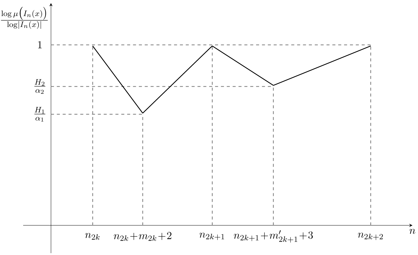
In fact, it has been proven that when  $k$ is large enough, between
 $n_{2k}$ and
 $n_{2k+2}$, the sequence
 $\frac{\log\mu\left(I_n(x)\right)}{\log \lvert I_n(x)\rvert}$ has two local minima at positions
 $n_{2k}+m_{2k}+2$ and
 $n_{2k+1}+m'_{2k+1}+3$. However, the limits exist for both subsequences
 $\{n_{2k}+m_{2k}+2\}_{k\geqslant0}$ and
 $\{n_{2k+1}+m'_{2k+1}+3\}_{k\geqslant0}$. Hence, the lower limit of the sequence
 $\frac{\log\mu(I_n(x))}{\log \lvert I_n(x)\rvert}$ is the minimum of these two limits. The analysis will be illustrated in Figure 8.
The asymptotic behaviour of the sequence  $\left\{\frac{\log\mu(I_n(x))}{\log \lvert I_{n}(x)\rvert}\right\}_{n\geqslant 1}$.

4.4. Proof of Theorem 2.3
Now, we are ready to give the final proof of Theorem 2.3.
Proof of Theorem 2.3
First note that if  $\textbf{H} \notin [\textbf{0}, \boldsymbol{\alpha}]$, then the equality of the spectrum in this region is immediate since the support of a bivariate spectrum trivially is included in the product of the supports of each function.
Now, we establish the multivariate multifractal spectrum on the union  ${\rm DL}$. If
 $\textbf{H}\in\left\{(0,H_2): H_2\in \left(0,\frac{\alpha_2}{\Delta(y)}\right]\right\}\cup\left\{(H_1,0): H_1\in \left(0,\frac{\alpha_1}{\Delta(y)}\right]\right\}$, then by Proposition 3.2, the Hausdorff dimension of
 $E_1(H_1)$ or
 $E_2(H_2)$ is
 $0$. Moreover, one checks directly that on these two sides of rectangle, the intersection
 $E_1(H_1)\cap E_2(H_2)$ is nonempty. Hence,
 \begin{equation*}
\dim_H\big(E_1(H_1)\cap E_2(H_2)\big)=0.
\end{equation*}
Suppose now  $\textbf{H}$ lies on the diagonal
 $\left\{\textbf{H} : \ H_1\in [0,{\alpha_1}] \mbox{and } H_2=\frac{{\alpha_2}}{{\alpha_1}} H_1\right\}$ of the rectangle
 $[\textbf{0}, \boldsymbol{\alpha}]$. Then,
 \begin{equation*}\delta := \min\left\{\frac{H_1}{{\alpha_1}},\frac{H_2}{{\alpha_2}}\right\}=\frac{H_1}{{\alpha_1}}=\frac{H_2}{{\alpha_2}}. \end{equation*}
It follows from classical ubiquity arguments, see [Reference Jaffard13], that there exists a  $\delta$-dimensional gauge function such that the corresponding Hausdorff measure is positive. Note that
 \begin{equation*} E_{y}(\textbf{H})=E_{1}(H_1) \cap E_{2}(H_2) = E_{y}^{\leqslant} (\textbf{H}) - \bigcup_{H \lt H_1} E^{\leqslant} ({H_1}) - \bigcup_{H \lt H_2} E^{\leqslant}_y ({H_2}) . \end{equation*}
Since the two unions on the right-hand side can be written as countable union, each of which being of dimension strictly less than  $\delta$, it follows that, for the
 $\delta$-dimensional gauge function considered above, the Hausdorff measures of these unions vanishes, so that
 \begin{equation}\mbox{if }\quad \frac{H_1}{{\alpha_1}}= \frac{H_2}{{\alpha_2}}, \quad \mbox{then} \qquad
\dim_H ( E_{1}(H_1) \cap E_{2}(H_2) ) =\min\left\{\frac{H_1}{{\alpha_1}},\frac{H_2}{{\alpha_2}}\right\}.
\end{equation}
This establishes the multivariate multifractal spectrum of Theorem 2.3 on the diagonal.
In the following, we will establish the multivariate multifractal spectrum on the rectangle
 \begin{equation*}\widetilde{K}_y= \left(0,\frac{{\alpha_1}}{\Delta (y)}\right]\times \left(0,\frac{{\alpha_2}}{\Delta (y)}\right]. \end{equation*}
The upper bound is easy to obtain; indeed, note that
 \begin{equation*}
\begin{aligned}
E_{y}(\textbf{H})\subset E_{1}(H_1),\\
E_{y}(\textbf{H})\subset E_{2}(H_2).
\end{aligned}
\end{equation*}
Then, by Proposition 3.2, for any  $\textbf{H} \in [\mathbf{0},\boldsymbol{\alpha}]$, the bivariate multifractal spectrum of Lévy functions
 $L_{{\alpha_1}}$ and
 $L_{\alpha_2}^{y}$ satisfies
 \begin{equation}
\dim_H\left(E_{y}(\textbf{H})\right)\leqslant \min\left\{\frac{H_1}{{\alpha_1}},\frac{H_2}{{\alpha_2}}\right\}.
\end{equation}
For the lower bound, it follows by combining (4.18), (4.25) and Lemma 3.3 that
 \begin{equation}
\dim_H\left(E_{y}(\textbf{H})\right)\geqslant\min\left\{\frac{H_1}{{\alpha_1}},\frac{H_2}{{\alpha_2}}\right\}.
\end{equation}
Finally, the multivariate multifractal spectrum on the rectangle  $\widetilde{K}_y$ follows directly from (4.27) and (4.28).
This also completes the proof of Theorem 2.3.
5. Dichotomy of the size of
$E_{y}(\textbf{H})$lg

In this section, we prove Theorem 2.5 which shows that the sets  $E_{y}(\textbf{H})$ are either empty or of minimal dimension.
Proof of Theorem 2.5
Let us consider the level set
 \begin{equation*}
\begin{aligned}
E_{y}(\textbf{H})=\left\{x \in \mathbb{R}:\Delta(x) = \frac{{\alpha_1}}{H_1}, \Delta(x-y)=\frac{{\alpha_2}}{H_2}\right\},
\end{aligned}
\end{equation*}
where  $\textbf{H}\in[\textbf{0},\boldsymbol{\alpha}] {\backslash} K_y$.
The  $b$-ary expansion of
 $y$ is written as
 $\theta_1\theta_2\theta_3\cdots$. By revisiting the proof of Theorem 2.3, the lower bound is based on the construction of a Cantor-type set, which is defined by using the sequence
 $\{n_k\}$. That is, the spectrum is the minimum of the spectra of the two Lévy functions, respectively, once there exists a sequence which may depend on
 $y$ and
 $\textbf{H}$, such that
 $\frac{kn_k}{n_{k+1}}\to 0,(k\to\infty),$ and
(i)
$\forall l\in \left[n_{2k},n_{2k}+n_{2k}\left\lfloor\left(\frac{\alpha_1}{H_1}-1\right)\right\rfloor\right]$, the length of the block of
$0$’s followed by
$\theta_l$ is less than or equal to
$\left\lfloor l\left(\frac{\alpha_2}{H_2}-1\right)\right\rfloor$.(ii)
$\forall l\in \left[n_{2k+1},n_{2k+1}+n_{2k+1}\left\lfloor\left(\frac{\alpha_2}{H_2}-1\right)\right\rfloor\right]$, the length of the block of
$0$’s followed by
$\theta_l$ is less than or equal to
$\left\lfloor l\left(\frac{\alpha_1}{H_1}-1\right)\right\rfloor$.


There will be two cases.
Case 1:  ${H_2} \lt \frac{\alpha_2H_1}{\alpha_1}$.
Suppose there exist infinitely many  $n$ such that for all
 ${l\in \left[n, \left\lfloor n\left(\frac{\alpha_2}{H_2}-1\right)\right\rfloor+n\right]}$, the length of the block of 0’s in the
 $b$-ary expansion of
 $y$ followed by
 $\theta_l$ is less than or equal to
 $\left\lfloor l\left(\frac{\alpha_1}{H_1}-1\right)\right\rfloor$. Then
 $n_{2k}$ can be taken as an infinite subsequence of these
 $n$’s. Hence, condition (ii) holds. On the other hand, by
 $H_2 \lt \frac{\alpha_2H_1}{\alpha_1}$, condition (i) holds automatically. Thus, by the same proof as in Theorem 2.3, a Cantor-type subset of
 $E_{y}(\textbf{H})$ can be constructed, and it follows that
 $
\mathcal{D}_{y}(\textbf{H})=
\min\left\{\frac{H_1}{{\alpha_1}}, \frac{H_2}{{\alpha_2}}\right\}.
$
Otherwise, for any sufficiently large  $n$, there exist
 $l_n \in \left[n, \left\lfloor n\left(\frac{\alpha_2}{H_2}-1\right)\right\rfloor+n\right]$, such that the length of the block of 0’s followed by
 $\theta_{l_n}$ is larger than
 $\left\lfloor l_n\left(\frac{\alpha_1}{H_1}-1\right)\right\rfloor$. For any
 $x\in E_{y}(\textbf{H})$, it holds that
 $\Delta (x-y)=\frac{\alpha_2}{H_2}$. Then, there exist infinitely many
 $n'$ such that the
 $b$-ary expansion of
 $x$ satisfies
 \begin{equation*}\varepsilon_{n'+1}\varepsilon_{n'+2}\cdots\varepsilon_{n'+\left\lfloor n'\left(\frac{\alpha_2}{H_2}-1\right)\right\rfloor}=\theta_{n'+1}\theta_{n'+2}\cdots\theta_{n'+\left\lfloor n'\left(\frac{\alpha_2}{H_2}-1\right)\right\rfloor}.\end{equation*}
Thus, for infinitely many  $n'$,
 \begin{equation*}
\lVert b^{n'}x \rVert \lt \frac{1}{b^{\left\lfloor n'\left(\frac{{\alpha_1}}{H_1}-1\right)\right\rfloor}},
\end{equation*}
which implies that
 \begin{equation*}
\Delta (x) \gt \frac{\alpha_1}{H_1}.
\end{equation*}
This contradicts the definition of the level set  $E_{y}(\textbf{H})$ which asks that
 $\Delta (x) = \frac{{\alpha_1}}{H_1}$. Therefore, such
 $x$ does not exist and the level set
 $E_{y}(\textbf{H})$ is empty, leading to the conclusion that the value of the bivariate multifractal spectrum is
 $-\infty$.
Case 2: 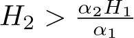 ${H_2} \gt \frac{\alpha_2H_1}{\alpha_1}$.
Suppose there exist infinitely many  $n$ such that for all
 ${l\in \left[n, \left\lfloor n\left(\frac{\alpha_1}{H_1}-1\right)\right\rfloor+n\right]}$, the length of the block of 0’s in the
 $b$-ary expansion of
 $y$ followed by
 $\theta_l$ is less than or equal to
 $\left\lfloor l\left(\frac{\alpha_2}{H_2}-1\right)\right\rfloor$. Then
 $n_{2k+1}$ can be taken as an infinite subsequence of these
 $n$’s. Hence, condition (i) is true. On the other hand, by
 $H_2 \gt \frac{\alpha_2H_1}{\alpha_1}$, condition (i) holds automatically. Thus, by the same proof as in Theorem 2.3, a Cantor-type subset of
 $E_{y}(\textbf{H})$ can be constructed, and it holds that
 $
\mathcal{D}_{y}(\textbf{H})=
\min\left\{\frac{H_1}{{\alpha_1}}, \frac{H_2}{{\alpha_2}}\right\}.
$
Otherwise, for any sufficiently large  $n$, there exist
 $l_n \in \left[n, \left\lfloor n\left(\frac{\alpha_1}{H_1}-1\right)\right\rfloor+n\right]$, such that the length of the block of 0’s followed by
 $\theta_{l_n}$ is larger than
 $\left\lfloor l_n\left(\frac{\alpha_2}{H_2}-1\right)\right\rfloor$. For any
 $x\in E_{y}(\textbf{H})$, it follows that
 $\Delta (x)=\frac{\alpha_1}{H_1}$. Then, there exist infinitely many
 $n'$ such that the
 $b$-ary expansion of
 $x$ satisfies
 \begin{equation*}\varepsilon_{n'+1}\varepsilon_{n'+2}\cdots\varepsilon_{n'+\left\lfloor n'\left(\frac{\alpha_1}{H_1}-1\right)\right\rfloor}=0^{\left\lfloor n'\left(\frac{\alpha_1}{H_1}-1\right)\right\rfloor}.\end{equation*}
Thus, for infinitely many  $n'$,
 \begin{equation*}
\lVert b^{n'}(x-y) \rVert \lt \frac{1}{b^{\left\lfloor n'\left(\frac{{\alpha_2}}{H_2}-1\right)\right\rfloor}},
\end{equation*}
which implies that
 \begin{equation*}
\Delta (x-y) \gt \frac{\alpha_1}{H_1}.
\end{equation*}
This contradicts the definition of the level set  $E_{y}(\textbf{H})$ which asks that
 $\Delta (x-y) = \frac{{\alpha_2}}{H_2}$. Therefore, such
 $x$ does not exist and the level set
 $E_{y}(\textbf{H})$ is empty, leading to the conclusion that the value of the bivariate multifractal spectrum is
 $-\infty$.
6. Proof of Propositions 2.6 and 2.7
Proof of Proposition 2.6
Let  $l_{i+1}=\lfloor l_{i}\eta\rfloor$ and suppose
 $y$ has
 $b$-ary expansion
 $\theta_1\theta_2\theta_3\cdots$. We consider
 \begin{equation}
\begin{aligned}
E_{y}(\textbf{H})&=\left\{x \in \mathbb{R}:\Delta(x) = \frac{{\alpha_1}}{H_1}\right\}\cap\left\{x \in \mathbb{R}: \Delta(x-y)=\frac{{\alpha_2}}{H_2}\right\},
\end{aligned}
\end{equation}
where  $\textbf{H}\in[\textbf{0},\boldsymbol{\alpha}] {\backslash} K_y.$
We will show that if
 \begin{equation}
\frac{{\alpha_2}{H_1}^2}{{\alpha_1}^2} \lt H_2 \lt \frac{{\alpha_2}}{{\alpha_1}}H_1,\ \text{and}\
\frac{\alpha_1}{\eta} \lt H_1\leqslant \alpha_1,
\end{equation}
then the conditions (i) and (ii) are satisfied. Hence, by following the proof as in Theorem 2.3, a Cantor-type set of  $E_{y}(\textbf{H})$ will be constructed and it follows that
 $
\mathcal{D}_{y}(\textbf{H})=
\min\left\{\frac{H_1}{{\alpha_1}}, \frac{H_2}{{\alpha_2}}\right\}.
$
In fact, if (6.2) holds, since  $\frac{{\alpha_2}{H_1}^2}{{\alpha_1}^2} \lt H_2$, then for all large
 $l_{i+1}$, it holds that
 \begin{equation*}
l_{i+1}\frac{H_1}{\alpha_1} \lt l_{i+1} \frac{\alpha_1H_2}{\alpha_2H_1}.
\end{equation*}
and there exists at least an integer  $n_i$ satisfying
 \begin{equation}
l_{i+1}\frac{H_1}{\alpha_1} \leqslant n_i\leqslant l_{i+1} \frac{\alpha_1H_2}{\alpha_2H_1},
\end{equation}
i.e.
 \begin{equation*}
\begin{aligned}
&l_{i+1}\leqslant n_i \frac{H_1}{{\alpha_1}},
\\ &n_i\leqslant l_{i+1}\frac{{\alpha_1}H_2}{{\alpha_2}H_1}.
\end{aligned}
\end{equation*}
Thus,
 \begin{equation}
\begin{aligned}
&l_{i+1}-n_i\leqslant \left\lfloor n_i\left(\frac{{\alpha_1}}{H_1}-1\right)\right\rfloor,\\ &
n_i+\left\lfloor n_i\left(\frac{{\alpha_2}}{H_2}-1\right)\right\rfloor-l_{i+1} \leqslant \left\lfloor l_{i+1}\left(\frac{{\alpha_1}}{H_1}-1\right)\right\rfloor.
\end{aligned}
\end{equation}
Therefore, by (6.4), there exists a subsequence of  $\{n_{i}\}$ which is still denoted as
 $\{n_{i}\}$, such that
 $\frac{in_i}{n_{i+1}}\to 0, (i\to\infty),$ and for all
 $p\in \left[n_{i}, \left\lfloor n_{i}\left(\frac{\alpha_2}{H_2}-1\right)\right\rfloor+n_{i}\right]$, the length of the block of 0’s followed by
 $\theta_p$ in the
 $b$-ary expansion of
 $y$ is less than or equal to
 $\left\lfloor l\left(\frac{\alpha_1}{H_1}-1\right)\right\rfloor$. Take
 $\{n_i\}$ as the sequence
 $\{n_{2k}\}$ in the proof of Theorem 2.3. Then condition (i) holds. On the other hand, by the assumption
 $H_2 \lt \frac{\alpha_2H_1}{\alpha_1}$, condition (ii) holds trivially. Then by taking the same proof as in Theorem 2.3, we can conclude that
 $
\mathcal{D}_{y}(\textbf{H})=
\min\left\{\frac{H_1}{{\alpha_1}}, \frac{H_2}{{\alpha_2}}\right\}.
$
Now, we will show that if
 \begin{equation*}
0\leqslant H_2\leqslant \frac{{\alpha_2}{H_1}^2}{{\alpha_1}^2}\ \text{and}\ \frac{\alpha_1}{\eta} \lt H_1\leqslant \alpha_1,
\end{equation*}
then the condition (ii) can never be satisfied. It then follows that  $E_{y}(\textbf{H})=\emptyset $.
In fact, for any  $i$ and
 $p\in[l_i, l_{i+1})$, if
 $l_i\leqslant p\leqslant \frac{l_{i+1}H_1}{\alpha_1},$ it holds that
 \begin{equation}
l_{i+1}-p \geqslant \left\lfloor p\left(\frac{{\alpha_1}}{H_1}-1\right)\right\rfloor.
\end{equation}
If  $p \gt \frac{l_{k+1}H_1}{\alpha_1},$ then by
 $H_2\leqslant \frac{{\alpha_2}{H_1}^2}{{\alpha_1}^2}$, it follows that
 \begin{equation*}
p \gt \frac{l_{k+1}\alpha_1H_2}{\alpha_2H_1}.
\end{equation*}
Hence
 \begin{equation}
p+\left\lfloor p\left(\frac{{\alpha_2}}{H_2}-1\right)\right\rfloor-l_{k+1} \gt \left\lfloor l_{k+1}\left(\frac{{\alpha_1}}{H_1}-1\right)\right\rfloor.
\end{equation}
By (6.5) and (6.6), for any sufficiently large  $n$, there exist
 $p_n\in \left[n, \left\lfloor n\left(\frac{\alpha_2}{H_2}-1\right)\right\rfloor+n\right]$, such that the length of the block of 0’s in the
 $b$-ary expansion of
 $y$ followed by
 $\theta_{p_n}$ is larger than
 $\left\lfloor p_n\left(\frac{\alpha_1}{H_1}-1\right)\right\rfloor$. Note that for any
 $x\in E_{y}(\textbf{H})$, it holds that
 $\Delta (x-y)=\frac{\alpha_2}{H_2}$. Then there exist infinitely many
 $n'$ such that the
 $b$-ary expansion
 $\varepsilon_1\varepsilon_2\cdots$ of
 $x$ satisfies
 \begin{equation*}\varepsilon_{n'+1}\varepsilon_{n'+2}\cdots\varepsilon_{n'+\left\lfloor n'\left(\frac{\alpha_2}{H_2}-1\right)\right\rfloor}=\theta_{n'+1}\theta_{n'+2}\cdots\theta_{n'+\left\lfloor n'\left(\frac{\alpha_2}{H_2}-1\right)\right\rfloor}.\end{equation*}
Hence, for infinitely many  $n'$, it follows that
 \begin{equation*}
\lVert b^{n'}x \rVert \lt \frac{1}{b^{\left\lfloor n\left(\frac{{\alpha_1}}{H_1}-1\right)\right\rfloor}}.
\end{equation*}
This implies
 \begin{equation*}
\Delta (x) \gt \frac{\alpha_1}{H_1},
\end{equation*}
which contradicts the definition of the level set asking that  $\Delta(x) = \frac{{\alpha_1}}{H_1}$. Therefore, the level set is empty.
Similarly, if  $\frac{{\alpha_1}{H_2}^2}{{\alpha_2}^2} \lt H_1 \lt \frac{{\alpha_1}}{{\alpha_2}}H_2,$ and
 $\frac{\alpha_2}{\eta} \lt H_2\leqslant \alpha_2$, then
 \begin{equation*}
\mathcal{D}_{y}(\textbf{H})=\min\left\{\frac{H_1}{{\alpha_1}}, \frac{H_2}{{\alpha_2}}\right\}.
\end{equation*}
If  $0\leqslant H_1\leqslant\frac{{\alpha_1}{H_2}^2}{{\alpha_2}^2}$ and
 $\frac{\alpha_2}{\eta} \lt H_2\leqslant \alpha_2$, then
 $E_{y}(\textbf{H})=\emptyset$.
Proof of Proposition 2.7
We consider the level set  $E_{y}(\textbf{H})$ for any
 $\textbf{H}\in [\mathbf{0},\boldsymbol{\alpha}]$. Let
 $n_i=\lfloor l_i\eta\rfloor$, for any
 $i$. The length of the block of 0’s followed by
 $\theta_{n_i}$ in the
 $b$-ary expansion of
 $y$ is 1. Then, a subsequence can be extracted from
 $\{n_i\}$ containing infinitely many terms which is still denoted as
 $\{n_{i}\}$ satisfying
 \begin{equation*}
\frac{i\cdot n_i}{n_{i+1}}\to 0, (i\to\infty),
\end{equation*}
and for each  $p\in \left[n_i, n_i+\max \left\{\left\lfloor {n_i}\left(\frac{{\alpha_1}}{H_1}-1\right)\right\rfloor,\left\lfloor {n_i}\left(\frac{{\alpha_2}}{H_2}-1\right)\right\rfloor\right\} \right]$,
 \begin{equation*}
\|b^{p}y\| \gt \frac{1}{b^{\min\left\{\left\lfloor {p}\left(\frac{{\alpha_1}}{H_1}-1\right)\right\rfloor,\left\lfloor {p}\left(\frac{{\alpha_2}}{H_2}-1\right)\right\rfloor\right\}} }.
\end{equation*}
Hence, conditions (i) and (ii) are satisfied. Then, by taking the same proof as that of Theorem 2.3, we can construct a Cantor-type subset of  $E_{y}(\textbf{H})$ and deduce that
 \begin{equation*}
\mathcal{D}_{y}(\textbf{H})=
\min\left\{\frac{H_1}{{\alpha_1}}, \frac{H_2}{{\alpha_2}}\right\}.
\end{equation*}
7. Conclusion
Let us first discuss the choice of the Hölder exponent for the analysis of Lévy functions. This is, in fact, motivated by the fact that if  $ \alpha \gt 0$ then the function
 $L_\alpha$ is locally bounded, so that there is no need to have recourse to the regularity exponent fitted to a more general setting, such as
 $p$-exponents, which only require that
 $f$ is locally
 $p$-integrable (i.e.
 $f \in L^p_{loc}$). However, the question can be raised if we allow to take negative values for
 $\alpha$. Indeed, in this case, the series still converges in the sense of distributions (see [Reference Jaffard, Melot, Leonarduzzi, Wendt, Abry, Roux and Torres22], or, more simply, remark that a formal term by term integration of sufficiently large order yields a normally convergent series), and one can wonder if a multifractal analysis of these generalized Lévy functions can be performed using
 $p$-exponents.
Let us focus on the case  $b=2$. Indeed, in this case, one can simply compute the coefficients of the dyadic Lévy functions on the Haar basis, which allows to determine for which values of
 $p$ it belongs
 $L^p_{loc} $. Let us first recall the definition of Haar basis. Let
 $ \varphi = 1_{[0,1]} $ and let
 \begin{equation}
\psi (x) = \varphi (2 x)- \varphi (2 x-1), \quad \forall x \in \mathbb{R}.\end{equation}
The Haar basis on  $[0,1]$ is the orthonormal basis of
 $L^2( [0,1]
) $ composed of the functions
 \begin{equation}
\left\{
\begin{array}{ll}
\varphi (x ) & \\
2^{j/2} \psi (2^jx
-k) & \mbox{for } j\geqslant0\,\, \mbox{and } k\in \{0, \cdots 2^j-1\} .
\end{array}
\right.
\end{equation}
We denote by  $c_{j,k}$ the coefficients of a function
 $f$ on this orthonormal basis. Let us compute the coefficients of the dyadic Lévy functions on the Haar basis. Let
 \begin{equation*}g_l (x) = \{2^l x \}, \quad \forall x \in \mathbb{R}.\end{equation*}
If  $j \lt l$, then the average of
 $g_l$ on dyadic intervals of length at least
 $2^{-l +1}$ vanishes. It follows that
 $ \lt \psi_{j,k} | g_l \gt =0$. If
 $j \geqslant l$, then
 $g_l$ is an affine function of slope
 $2^l$ on the support of
 $\psi_{j,k} $, and an immediate computation yields
 \begin{equation*} \lt \psi_{j,k} | g_l \gt = -\frac{1}{4} 2^{l-j} .
\end{equation*}
It follows that the wavelet coefficients of  $L_{\alpha}^2$ are
 \begin{equation*}
c_{j,k} = -\frac{1}{4} 2^{-j/2} \sum_{l=0}^j 2^{(1-\alpha ) l } ,
\end{equation*}
for which, assuming  $\alpha \lt 1$, we can write
 \begin{equation*}
c_{j,k} = C_1 2^{-\alpha j } + C_2 2^{- j },\quad \text{with}\quad C_1, C_2\ \text{being two constants}.
\end{equation*}
Recall that, for  $p \in (1, \infty)$, a norm equivalent to the
 $L^p$ norm of a function
 $f$ is given by
 \begin{equation}
\parallel f \parallel^p_{L^p} = \left\lVert \left( \sum_j \sum_k | c_{j,k} |^2 2^j \chi_\lambda \right)^{1/2} \right\lVert^p_{L^p},
\end{equation}
where  $\lambda$ denotes the dyadic interval
 $\lambda = [ k 2^{-j},\; (k +1)2^{-j} ] $. For
 $f =L_{\alpha}$, the double sum in the parenthesis in (7.3) boils down to
 \begin{equation*} \sum_j 2^{-2\alpha j} ,\end{equation*}
which diverges if  $\alpha \lt 0$. We conclude that using
 $p$-exponents does not allow to deal with a larger range of values of
 $\alpha$; indeed, as soon as
 $\alpha \lt 0 $, the dyadic Lévy functions
 $L_{\alpha}$ are Schwartz distributions which do not belong to any
 $L^p$ space.
The entire bivariate multifractal spectrum of Lévy function  $L_{\alpha_1}$ and translated Lévy function
 $L_{\alpha_2}^{y}$ for almost every
 $y$ was determined, that is,
 \begin{equation*}
\begin{aligned}
\mathcal{D}_{y}(\textbf{H})=
\begin{cases}
\min\left\{\frac{H_1}{{\alpha_1}}, \frac{H_2}{{\alpha_2}}\right\}, & \quad {\rm if}\ \textbf{H}\in [\mathbf{0},\boldsymbol{\alpha}],\\
-\infty & \quad {\rm else}.
\end{cases}
\end{aligned}
\end{equation*}
For other values of  $y$, the spectrum in the region
 $K_y$ was determined. For values outside
 $K_y$, we were able to prove that the spectrum is either the minimum of the spectra of the two Lévy functions, respectively, or
 $-\infty$, this leaves open the determination of the bivariate multifractal spectrum on the region
 $ [\textbf{0},\boldsymbol{\alpha}] \setminus K_y$.
From the multifractal analysis of Lévy functions, it appears that the spectrum is consistently either the empty set or the formula of large intersection as given by (1.4). This result allows to conjecture that, under mild hypotheses, the bivariate multifractal spectra of pairs of jump functions exhibit a distinct structure: the spectrum at the values given by the bivariate level sets is either  $-\infty$ or corresponds to the minimum of the individual spectra of the two functions. We will come back to this question in [Reference Jaffard, Liao and Zhang20].
Another important direction of research is to extend the present work to the bivariate multifractal analysis of Lévy functions  $L_{\alpha_1}^{b_1}$ and
 $L_{\alpha_2}^{b_2}$ with different bases
 $b_1$ and
 $b_2$, respectively, where
 $b_1$ and
 $b_2$ are coprime. We expect that this would yield further insights into how varying the base parameters affects the multifractal properties of Lévy functions. By investigating functions with different bases, we aim to develop a more generalized framework for multifractal spectrum, potentially uncovering new phenomena that could be applicable to a broader class of functions. This work would not only deepen our theoretical understanding but also pave the way for practical applications in fields where multifractal analysis is utilized, and in particular for applications where possible shifts of (known or unknown quantities) may occur between the data under analysis.
Moreover, we are interested in Hecke’s functions
 \begin{equation*}
H_{\alpha}(x)=\frac{\{nx\}}{n^{\alpha}} .
\end{equation*}
A next interesting challenge is to perform the multivariate multifractal analysis of Hecke’s function  $H_{\alpha_1}$ and the translated Hecke’s function
 $H_{\alpha_2}^y$ which satisfies
 $H_{\alpha_2}^y=H_{\alpha_2}(\cdot-y)$ for a given translation parameter
 $y\in \mathbb{R}$, which means that we aim at obtaining the bivariate multifractal spectrum of Hecke’s translated functions.
Acknowledgements
The authors would like to thank the referees for their remarks and suggestions that led to important improvements in the redaction of this article. Lingmin Liao was partially supported by the Fundamental Research Funds for the Central Universities of China (1301/413100126).