1. Introduction
Large buildings, including power stations, industrial plants, data centres and hospitals, generate large amounts of low-temperature waste thermal energy. Seasonal fluctuations in the demand for heating and initiatives for energy efficiency motivate interest in the potential for inter-seasonal storage and recovery of this thermal energy (Mackay Reference Mackay2008). Aquifer thermal energy storage (ATES) uses shallow permeable aquifers to store this thermal energy (Bakema et al. Reference Bakema, Snijders and Nordell1994). For example, such a system has been used effectively at Linieken Noord Antwerper hospital in Belgium (Vanhoudt et al. Reference Vanhoudt, Desmedt, Van Bael, Robeyn and Hoes2011). Several models have been developed to explore the dispersal of thermal energy in aquifers, with particular interest in the fraction of the thermal energy that can be recovered during the extraction cycle (Gringarten & Sauty Reference Gringarten and Sauty1975; Sauty et al. Reference Sauty, Gringarten, Fabris, Thiery, Menjoz and Landel1982a ,Reference Sauty, Gringarten, Menjoz and Landel b ; Dickinson et al. Reference Dickinson, Buik, Matthews and Snijders2009; Dudfield & Woods Reference Dudfield and Woods2012). These have investigated heat loss resulting from thermal conduction to the neighbouring strata and also the effects of buoyancy controlled flow, which influences the flow of the injected fluid and hence thermal energy.
One of the key challenges in such an open heat storage system concerns the potential for the extraction of original aquifer fluid, with the injected fluid, especially if the aquifer contains heavy metals or other contaminants which require special treatment at the surface. Moreover, the original aquifer fluid may contain dissolved minerals which precipitate at low pressure and may therefore lead to minerals forming and blocking the pipework. Hence, a focus of our work is to examine the composition of the extracted fluid (Dudfield & Woods Reference Dudfield and Woods2014).
Dudfield & Woods (Reference Dudfield and Woods2014) modelled the flow pattern in a confined saturated horizontal aquifer. They developed some experimental and theoretical models to quantify the fraction of injected fluid that is subsequently extracted. They identified that the fraction of injected fluid that is recovered on each cycle increases, and eventually nearly all of the injected fluid is then extracted during a cycle. The system has one controlling parameter,
 ${\it\Gamma}$
, the ratio of gravity driven flow and pressure driven flow, which determines the number of cycles required for the system to reach equilibrium. At early times, buoyancy slumping leads to the recovery of only a fraction of the injected fluid during each extraction cycle. The concentration of the original aquifer fluid that is extracted is initially
 ${\sim}O(0.1)$
, but becomes very small at long times. As
 ${\it\Gamma}$
decreases, the system is dominated by pressure driven flow, and more injected fluid is recovered during the extraction phases. In this paper we investigate the effects of the inclination of the aquifer, and we show that this leads to a phenomenologically different result due to the tendency of the injected fluid to run off downslope. As a result, the flow adjusts until during each extraction cycle a constant fraction of original aquifer fluid is produced.
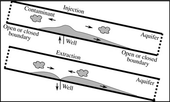
In this paper we model the case in which a single well is used for both injection and extraction in a laterally extensive inclined aquifer of relatively small vertical extent, and fluid is injected and extracted at the base of the inclined aquifer, as shown in figure 1, § 2. We assume that the density of the injected fluid is greater than that of the reservoir fluid, and using a series of theoretical models we explore how the flow pattern and the fraction of injected fluid that is extracted evolve from cycle to cycle and are a function of two controlling parameters,
 ${\it\Gamma}=H(S\cos ({\it\theta}){\it\phi}^{2}/{\it\tau}Q^{2})^{1/3}$
and
 ${\it\Pi}=HS\sin ({\it\theta}){\it\phi}/Q$
, where
 $S$
is the buoyancy speed of the dense fluid,
 $H$
is the vertical extent of the aquifer,
 ${\it\theta}$
is the porosity of the aquifer,
 ${\it\tau}$
is the time period of injection and
 $Q$
is the volume injected per unit length of the well. We assume that the aquifer is of finite vertical extent, and we explore the two cases in which there is an open boundary either downslope or upslope of the source, with the other boundary being sealed, as shown in figure 1.
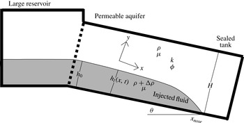
Illustration of injection and extraction of fluid into and from a permeable aquifer between two impermeable layers. The dashed lines represent open or closed boundaries far from the injection and extraction well. The arrows show the movement of both the injected fluid, shaded in, and the original aquifer fluid, and the wavy area shows a region containing contaminants which is explored in § 6.

Dispersive mixing between the injected and reservoir fluids can occur and may lead to a region of intermediate composition (Bear & Cheng Reference Bear and Cheng2010; Woods Reference Woods2015). The mixing time scales as
 $t_{D}\sim H^{2}/D$
, where
 $H\sim O(10)$
m is the aquifer thickness and
 $D\sim O(10^{-8}){-}O(10^{-10})~\text{m}^{2}~\text{s}^{-1}$
is the pore scale dispersion, and therefore
 $t_{D}\sim 10{-}1000$
years. Although such mixing will eventually become important after many cycles, in this present analysis, in which we are primarily interested in the processes that occur over the first few inter-seasonal injection–extraction cycles,
 $t\ll t_{D}$
, we neglect the effect of hydrodynamic dispersion between the injected and original fluid and assume that there is a sharp interface (Huppert & Woods Reference Huppert and Woods1995). However, it would be of interest to include this dispersion when modelling the long-time dynamical behaviour of the flow (Szulczewski & Juanes Reference Szulczewski and Juanes2013; Woods Reference Woods2015).
In §§ 3 and 4 we explore the cases in which there is an open boundary either upslope (§ 3) or downslope (§ 4) of the source, with the other boundary being sealed, respectively. We show that near the well an oscillatory flow structure develops, while in the far-field downslope a tongue of injected dense fluid propagates downwards with a constant flux. This drives a corresponding inflow of reservoir fluid towards the well.
In § 5 we show that the far-field downslope flow of injected fluid asymptotes to one of a family of exchange flows that develops when a reservoir of dense fluid located at
 $x=0$
, of depth
 $h_{0}\leqslant H$
, overlain by reservoir fluid, is connected to an inclined confined aquifer, in the region
 $x>0$
. We also show how the dimensionless thickness
 $g_{0}=h_{0}/H$
depends on
 ${\it\Gamma}$
and
 ${\it\Pi}$
.
In § 6 we investigate how the concentration of original aquifer that is extracted varies during an extraction cycle. We also explore the rate at which the original aquifer fluid migrates towards the well and thereby predict the time at which a region of contaminated fluid, originally located far from the well, may be transported to the well as a result of the periodic injection and extraction of fluid.
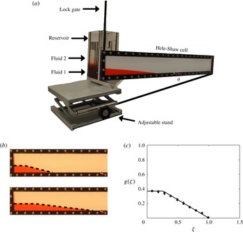
We test the predictions of these two cases and the exchange flow solution with a series of new laboratory experiments using a Hele-Shaw cell in § 7. In § 8 we draw some conclusions and discuss possible developments of this work.
2. Inclined confined aquifer
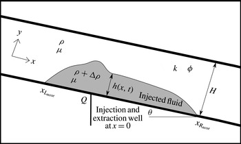
We consider the periodic injection of fluid of density
 ${\it\rho}+{\rm\Delta}{\it\rho}$
and viscosity
 ${\it\mu}$
into, and its extraction from, a saturated inclined aquifer, with period
 $2{\it\tau}$
and of volume flow rate per unit length
 $Q(t)$
, as shown in figure 2. The aquifer has porosity
 ${\it\phi}$
and permeability
 $k$
, has an impermeable inclined base, at angle
 ${\it\theta}$
to the horizontal, and initially is filled with fluid of the same viscosity
 ${\it\mu}$
but of density
 ${\it\rho}$
. We assume that the cross-aquifer thickness is
 $H$
. We focus on flows with a small aspect ratio (depth/length)
 ${\it\epsilon}\ll 1$
, in which case the flow is approximately one-dimensional and parallel to the boundary, and the vertical pressure may be assumed to be hydrostatic (Bear Reference Bear1988; Barenblatt, Entov & Ryzhik Reference Barenblatt, Entov and Ryzhik1990).
Schematic illustration of fluid in an aquifer of thickness
 $H$
, porosity
 ${\it\phi}$
, permeability
 $k$
and inclined at an angle
 ${\it\theta}$
to the horizontal, showing the position of the downslope,
 $x_{R_{nose}}(t)$
, and upslope,
 $x_{L_{nose}}(t)$
, leading edges of the injected fluid. The height of the fluid front is shown by
 $h(x,t)$
, with the injected fluid, of density
 ${\it\rho}+{\rm\Delta}{\it\rho}$
and viscosity
 ${\it\mu}$
, lying below the front while the reservoir fluid, of density
 ${\it\rho}$
and viscosity
 ${\it\mu}$
, lies above the front.

The current occupies the region
 $0\leqslant y\leqslant h(x,t)\leqslant H$
and
 $x_{L_{nose}}(t)\leqslant x\leqslant x_{R_{nose}}(t)$
, where
 $h(x_{L_{nose}}(t),t)=h(x_{R_{nose}}(t),t)=0$
. The hydrostatic pressure gradient has the form
 $$\begin{eqnarray}P(x,y,t)=\left\{\begin{array}{@{}ll@{}}p_{0}(x,t)-({\it\rho}+{\rm\Delta}{\it\rho})gy\cos ({\it\theta}),\quad & \text{if }0<y\leqslant h,\\ p_{0}(x,t)-({\it\rho}+{\rm\Delta}{\it\rho})gh\cos ({\it\theta})-g{\it\rho}(y-h)\cos ({\it\theta}),\quad & \text{if }h<y\leqslant H.\end{array}\right.\end{eqnarray}$$
Darcy’s law then gives the flow speeds
 $u_{1}$
below and
 $u_{2}$
above the interface as
 $$\begin{eqnarray}\displaystyle u_{1}\! & = & \displaystyle \!-\frac{k}{{\it\mu}}\left(\frac{\partial p_{0}}{\partial x}-({\it\rho}+{\rm\Delta}{\it\rho})g\sin ({\it\theta})\right),\end{eqnarray}$$
 $$\begin{eqnarray}\displaystyle u_{2}\! & = & \displaystyle \!-\frac{k}{{\it\mu}}\left(\frac{\partial p_{0}}{\partial x}-{\rm\Delta}{\it\rho}g\frac{\partial h}{\partial x}\cos ({\it\theta})-{\it\rho}g\sin ({\it\theta})\right),\end{eqnarray}$$
 $$\begin{eqnarray}\displaystyle [u_{1}h+u_{2}(h-H)]_{0^{-}}^{0^{+}}=Q(t)=\left\{\begin{array}{@{}ll@{}}Q\quad & \text{if }2n{\it\tau}<t\leqslant (2n+1){\it\tau},\\ -Q\quad & \text{if }(2n+1){\it\tau}<t\leqslant (2n+2){\it\tau}.\end{array}\right. & & \displaystyle\end{eqnarray}$$
We now assume that the flux is partitioned so that a fraction of the flux migrates upslope,
 $f$
, and downslope,
 $1-f$
, and therefore
 $$\begin{eqnarray}\displaystyle hu_{1}+(H-h)u_{2}={\it\lambda}=Q(t)\left\{\begin{array}{@{}ll@{}}f,\quad & \text{if }x>0,\\ -(1-f),\quad & \text{if }x<0.\end{array}\right. & & \displaystyle\end{eqnarray}$$
In §§ 3 and 4 we explore the two cases (i)
 $f=0$
, which represents a closed boundary in the downslope far field and an open boundary in the upslope far field, and (ii)
 $f=1$
, which represents an open boundary in the downslope far field and a closed boundary in the upslope far field, respectively.
Using (2.5), (2.2) and (2.3) become
 $$\begin{eqnarray}\displaystyle u_{1}\! & = & \displaystyle \!\frac{{\it\lambda}}{H}-\frac{k{\rm\Delta}{\it\rho}g}{{\it\mu}}\frac{H-h}{H}\left(\frac{\partial h}{\partial x}\cos ({\it\theta})-\sin ({\it\theta})\right),\end{eqnarray}$$
 $$\begin{eqnarray}\displaystyle u_{2}\! & = & \displaystyle \!\frac{{\it\lambda}}{H}-\frac{k{\rm\Delta}{\it\rho}g}{{\it\mu}}\frac{h}{H}\left(-\frac{\partial h}{\partial x}\cos ({\it\theta})+\sin ({\it\theta})\right).\end{eqnarray}$$
 $$\begin{eqnarray}\displaystyle \frac{\partial h}{\partial t}+\frac{1}{H{\it\phi}}\frac{\partial ({\it\lambda}h)}{\partial x} & = & \displaystyle S\cos ({\it\theta})\frac{\partial }{\partial x}\left(h\left(1-\frac{h}{H}\right)\left(\frac{\partial h}{\partial x}-\tan ({\it\theta})\right)\right),\end{eqnarray}$$
where
 ${\it\phi}S\cos ({\it\theta})=({\rm\Delta}{\it\rho}gk)/{\it\mu}\cos ({\it\theta})$
is a scale for the buoyancy driven speed.
During both the injection and extraction cycles, we require the height of the fluid at the source to be continuous. During the extraction cycle it is also possible that
 $h(0,t)=0$
, in which case a mixture of the two fluids may be produced, and in this case we require
 $\partial h/\partial t=0$
at
 $x=0$
. Therefore, using (2.5) combined with (2.6) and (2.7), the boundary conditions at
 $x=0$
take the form
 $$\begin{eqnarray}\displaystyle \begin{array}{@{}cl@{}}\displaystyle [h]_{0^{-}}^{0^{+}}=0, & \forall t,\\ \displaystyle -[u_{1}h]_{0^{-}}^{0^{+}}={\it\phi}S\cos ({\it\theta})\displaystyle \left[h\frac{\partial h}{\partial x}\right]_{0^{-}}^{0^{+}}\displaystyle =-Q, & \text{if }2n{\it\tau}<t\leqslant (2n+1){\it\tau},\\ \displaystyle -[u_{1}h]_{0^{-}}^{0^{+}}={\it\phi}S\cos ({\it\theta})\displaystyle \left[h\frac{\partial h}{\partial x}\right]_{0^{-}}^{0^{+}}=Q, & \displaystyle \text{if }(2n+1){\it\tau}<t\leqslant (2n+2){\it\tau}\text{ and }h>0,\\ \displaystyle \frac{\partial h}{\partial t}=0, & (2n+1){\it\tau}<t\leqslant (2n+2){\it\tau}\text{ and }h=0.\end{array} & & \displaystyle\end{eqnarray}$$
Finally, as an initial condition, at
 $t=0$
, we require that
 $h(x,t)=0$
.
It is convenient to introduce scalings for the flow in order to work with dimensionless variables. The natural time scale in this problem is
 ${\it\tau}$
, and the depth scale is
 $H$
, so that with an injected volume
 $Q{\it\tau}$
over one cycle, the characteristic length
 $L$
into the aquifer is
 $$\begin{eqnarray}L\sim \frac{Q{\it\tau}}{{\it\phi}H}.\end{eqnarray}$$
Using (2.10), we recast the system of equations in the dimensionless form
 $$\begin{eqnarray}h=HF\left(t^{\prime }=\frac{t}{{\it\tau}},{\it\eta}=\frac{xH{\it\phi}}{Q{\it\tau}}\right)\end{eqnarray}$$
and define the dimensionless down- and upslope edges of the current to have positions
 $$\begin{eqnarray}\displaystyle {\it\eta}_{R_{nose}}=\frac{x_{R_{nose}}H{\it\phi}}{Q{\it\tau}}, & & \displaystyle \text{where }F({\it\eta}_{R_{nose}},t^{\prime })=0,\end{eqnarray}$$
 $$\begin{eqnarray}\displaystyle {\it\eta}_{L_{nose}}=\frac{x_{L_{nose}}H{\it\phi}}{Q{\it\tau}}, & & \displaystyle \text{where }F({\it\eta}_{L_{nose}},t^{\prime })=0.\end{eqnarray}$$
 $V^{\prime }(t^{\prime })$
, as
 $$\begin{eqnarray}\displaystyle V^{\prime }(t^{\prime })=\frac{V(t)}{Q{\it\tau}}=\frac{{\it\phi}\displaystyle \int _{x_{L_{nose}}}^{x_{R_{nose}}}h\,\text{d}x}{Q{\it\tau}}=\int _{{\it\eta}_{L_{nose}}}^{{\it\eta}_{R_{nose}}}F\,\text{d}{\it\eta}. & & \displaystyle\end{eqnarray}$$
Equation (2.8) now becomes (cf. Gunn & Woods Reference Gunn and Woods2011)
 $$\begin{eqnarray}\displaystyle & & \displaystyle \displaystyle \frac{\partial F}{\partial t^{\prime }}+\left({\rm\Lambda}+{\it\Pi}(1-2F)\right)\frac{\partial F}{\partial {\it\eta}}={\it\Gamma}^{3}\frac{\partial }{\partial {\it\eta}}\left((1-F)F\frac{\partial F}{\partial {\it\eta}}\right),\nonumber\\ \displaystyle & & \displaystyle \displaystyle \qquad \text{where }{\it\Gamma}=H\left(\frac{S\cos ({\it\theta}){\it\phi}^{2}}{{\it\tau}Q^{2}}\right)^{1/3},{\it\Pi}=\frac{HS\sin ({\it\theta}){\it\phi}}{Q}\text{ and }{\rm\Lambda}={\it\lambda}/Q.\end{eqnarray}$$
Here,
 ${\it\Pi}$
is the ratio of the downslope buoyancy driven flux to the injection flux and
 ${\it\Gamma}$
represents the ratio of the vertical extent of the aquifer to the depth of a gravity current produced by a constant flux
 $Q$
after time
 ${\it\tau}$
in an unconfined aquifer.
We seek solutions of (2.15) for which
 $F=0$
at
 $t^{\prime }=0$
with the boundary conditions
 $$\begin{eqnarray}\displaystyle \left.\begin{array}{@{}cl@{}}\displaystyle [F]_{0^{-}}^{0^{+}}=0, & \forall t^{\prime },\\ \displaystyle \left[F\frac{\partial F}{\partial {\it\eta}}\right]_{0^{-}}^{0^{+}}\displaystyle =-\frac{1}{{\it\Gamma}^{3}}, & \text{if }2n<t^{\prime }\leqslant 2n+1,\\ \displaystyle \left[F\frac{\partial F}{\partial {\it\eta}}\right]_{0^{-}}^{0^{+}}\displaystyle =\frac{1}{{\it\Gamma}^{3}}, & \text{if }2n+1<t^{\prime }\leqslant 2n+2\text{ and }F>0,\\ \displaystyle \frac{\partial F}{\partial t^{\prime }}=0, & 2n+1<t^{\prime }\leqslant 2n+2\text{ and }\displaystyle F=0,\end{array}\right\} & & \displaystyle \text{at }{\it\eta}=0,\end{eqnarray}$$
 $$\begin{eqnarray}\displaystyle \text{and }F\rightarrow 0\text{ as }{\it\eta}\rightarrow \pm \infty . & & \displaystyle\end{eqnarray}$$
 $t^{\prime }$
and
 ${\it\eta}$
until the results were independent of grid size.
The advection term,
 ${\it\Pi}(1-2F)F^{\prime }$
, dominates the diffusion term,
 ${\it\Gamma}^{3}((1-F)FF^{\prime })^{\prime }$
, and balances the
 $\partial F/\partial t^{\prime }$
term in (2.15) provided that
 $$\begin{eqnarray}t^{\prime }\gg \frac{{\it\Gamma}^{3}}{{\it\Pi}^{2}}F_{C}=\frac{h_{C}\cot ({\it\theta})}{S\sin {\it\theta}{\it\tau}},\end{eqnarray}$$
where
 $F_{C}$
and
 $h_{C}$
are scales for
 $F$
and
 $h$
respectively, as we define in (3.1). This scaling follows by noting that
 ${\it\eta}$
scales like
 ${\it\Pi}t^{\prime }$
because the advection term is in balance with the
 $\partial F/\partial t^{\prime }$
term.
Let us define the average concentration of original aquifer fluid that is extracted during one cycle,
 $\bar{C}$
, to be
 $$\begin{eqnarray}\displaystyle \bar{C}(n) & = & \displaystyle 1-\frac{V_{out}}{V_{in}}=1-V^{\prime }(2n-1)+V^{\prime }(2n),\quad \text{where }n\in Z.\end{eqnarray}$$
Let us also define the long-time limit of average concentration of original aquifer fluid that is extracted over an extraction cycle as
 $$\begin{eqnarray}\displaystyle \mathscr{F}=\lim _{n\rightarrow \infty }\bar{C}(n). & & \displaystyle\end{eqnarray}$$
3. Open boundary located upslope from the injection well
In this section, we consider the case in which the upslope boundary is open, and the excess fluid from the injection–extraction cycle escapes and re-enters through this open boundary, see figure 1. We explore the details of the first few injection–extraction cycles and then show that the volume and the nose of the injection fluid increase linearly with
 $t^{\prime }$
at leading order. We then investigate the influence of
 ${\it\Gamma}$
and
 ${\it\Pi}$
in controlling the volume of injected fluid in the aquifer. To model the conservation of mass upslope and downslope from the injection extraction well, we use (2.5) and set
 $f=0$
.
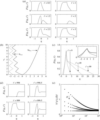
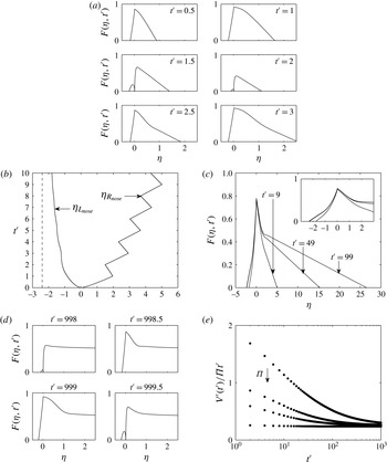
Profiles of the thickness,
 $F({\it\eta},t^{\prime })$
, as a function of the distance,
 ${\it\eta}$
, in the aquifer during the first and second injection cycles and the first extraction cycle,
 $0\leqslant t^{\prime }\leqslant 3$
, are shown in figure 3(a) at dimensionless times
 $t^{\prime }=0.5$
, 1, 1.5, 2, 2.5 and 3 for
 ${\it\Gamma}=0.5$
and
 ${\it\Pi}=0.4$
. Figure 3(b) shows how the positions of the downslope nose,
 ${\it\eta}_{R_{nose}}$
, and the upslope nose,
 ${\it\eta}_{L_{nose}}$
, vary as a function of time,
 $t^{\prime }$
, for
 ${\it\Gamma}=1$
and
 ${\it\Pi}=0.2$
. We see that the upslope nose oscillates due to the open boundary upslope of the injection and extraction well.
Figure 3(c) compares the profiles of the current at the end of the injection phases after many cycles are complete, namely at
 $t^{\prime }=9$
, 49 and 99, for
 ${\it\Gamma}=1$
and
 ${\it\Pi}=0.2$
. It may be seen that
 ${\it\eta}_{R_{nose}}(t^{\prime })$
continues to increase with time, indicating how the flow continues to spread downslope into the saturated rock. In figure 3(d) we show the variation of the current thickness,
 $F({\it\eta},t^{\prime })$
, as a function of the position,
 ${\it\eta}$
, during an injection–extraction cycle at long time (
 $t^{\prime }=998.0$
, 998.5, 999 and 999.5), for
 ${\it\Gamma}=0.5$
and
 ${\it\Pi}=0.4$
.
It may be seen, in figure 3(c,d), that the current organises itself into two regions. Near the source, there is a large-amplitude oscillation in the thickness of the current over each cycle, while beyond this region, the current largely involves a net outward flow associated with the sloping aquifer. The height of the interface between these two regions coincides approximately with the position at which the depths of the interfaces at the end of the injection phase and at the end of the extraction phase are equal, and we define this position and height as
 $$\begin{eqnarray}{\it\eta}={\it\eta}_{C}({\it\Gamma},{\it\Pi})=x_{C}\frac{H{\it\phi}}{Q{\it\tau}}\quad \text{and}\quad \frac{h_{C}}{H}=F_{C}({\it\Gamma},{\it\Pi})=\lim _{t^{\prime }\rightarrow \infty }F({\it\eta}_{C},t^{\prime }).\end{eqnarray}$$
For the lubrication approximation to be valid, as assumed in § 2, we need
 $h_{C}/x_{C}\ll 1$
. Using our full numerical solutions for
 $0.3\leqslant {\it\Gamma}\leqslant 10$
and
 $0.1\leqslant {\it\Pi}\leqslant 1$
, then in the case
 $H\sim 10$
m,
 ${\it\phi}\sim 0.1$
and
 $Q{\it\tau}\sim 10^{2}~\text{m}^{2}$
, the lubrication approximation is valid.
Numerical predictions. (a) The variation of the current thickness
 $F({\it\eta},t^{\prime })$
as a function of the position
 ${\it\eta}$
during the first and second injection cycles and the first extraction cycle, at dimensionless times
 $t^{\prime }=0.5$
, 1, 1.5, 2, 2.5 and 3, for
 ${\it\Gamma}=0.5$
and
 ${\it\Pi}=0.4$
. (b) The positions of the downslope nose,
 ${\it\eta}_{R_{nose}}$
, and the upslope nose,
 ${\it\eta}_{L_{nose}}$
, as a function of time,
 $t^{\prime }$
, for
 ${\it\Gamma}=1$
and
 ${\it\Pi}=0.2$
. The dashed line shows the upper limit of
 ${\it\eta}_{L_{nose}}$
as predicted by (3.4). (c) The variation of the current thickness
 $F({\it\eta},t^{\prime })$
as a function of the position
 ${\it\eta}$
at the end of the injection phases at
 $t^{\prime }=9$
, 49 and 99 for
 ${\it\Gamma}=1$
and
 ${\it\Pi}=0.2$
(the inset plot shows the profile shape near the extraction well). (d) The variation of the current thickness
 $F({\it\eta},t^{\prime })$
as a function of the position
 ${\it\eta}$
during an injection–extraction cycle at long time (
 $t^{\prime }=998.0$
, 998.5, 999 and 999.5), for
 ${\it\Gamma}=0.5$
and
 ${\it\Pi}=0.4$
. (e) The volume of the current scaled with
 ${\it\Pi}t^{\prime }$
,
 $V^{\prime }(t^{\prime })/{\it\Pi}t^{\prime }$
, as a function of time for
 ${\it\Gamma}=1$
and
 ${\it\Pi}=0.1$
,
 $0.2$
,
 $0.3$
and 1; the arrow shows the direction of increasing
 ${\it\Pi}$
.

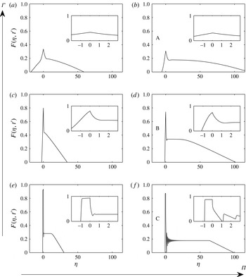
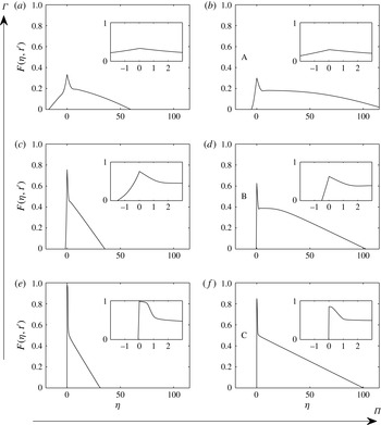
Numerical prediction of the variation of the current thickness
 $F({\it\eta},t^{\prime })$
as a function of the position
 ${\it\eta}$
at the end of the injection and extraction phases at
 $t^{\prime }=99$
for combinations of
 ${\it\Gamma}=3$
,
 ${\it\Pi}=0.3$
(a);
 ${\it\Gamma}=3$
,
 ${\it\Pi}=1$
(b);
 ${\it\Gamma}=1$
,
 ${\it\Pi}=0.3$
(c);
 ${\it\Gamma}=1$
,
 ${\it\Pi}=1$
(d);
 ${\it\Gamma}=0.3$
,
 ${\it\Pi}=0.3$
(e);
 ${\it\Gamma}=0.3$
,
 ${\it\Pi}=1$
(f); the large arrows show the directions for
 ${\it\Gamma}$
and
 ${\it\Pi}$
increase. The inset plots show the profile shape near the extraction well, showing that for
 ${\it\Gamma}=0.3$
and
 ${\it\Pi}=1$
the oscillations are not numerical errors. Points A, B and C are referred to in figure 5. Note the different scales in the
 $x$
and
 $y$
axes.

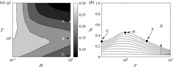
(a) Contour plot of the long-term limit (
 $t^{\prime }=1000$
) of
 $V^{\prime }(t^{\prime })/{\it\Pi}t^{\prime }\rightarrow V_{u}({\it\Gamma},{\it\Pi})$
, see (3.2). (b) The long-time limit (
 $t^{\prime }=1000$
) of the amount of original aquifer fluid compared with the injected fluid that is extracted during an extraction cycle,
 $\mathscr{F}$
, as a function of
 ${\it\Gamma}$
, for
 ${\it\Pi}=0.1$
to
 ${\it\Pi}=1$
in intervals of
 $0.1$
, with a vertical arrow showing the increase in
 ${\it\Pi}$
. A, B and C are denoted on (a) and (b) and are related to figure 4.

At long times the volume of the current grows linearly with time,
 $V(t^{\prime })\sim t^{\prime }$
. For example, in figure 3(e) we show the variation with time of the quantity
 $V(t^{\prime })/{\it\Pi}t^{\prime }$
at the end of each extraction cycle, for
 ${\it\Gamma}=1$
and
 ${\it\Pi}=0.1$
,
 $0.2$
,
 $0.3$
and 1. In each case
 $V(t^{\prime })/{\it\Pi}t^{\prime }$
becomes independent of time,
 $t^{\prime }$
, at large times, and in general we can define
 $$\begin{eqnarray}\displaystyle \lim _{t^{\prime }\rightarrow \infty }\frac{V^{\prime }(t^{\prime })}{{\it\Pi}t^{\prime }}=V_{u}({\it\Gamma},{\it\Pi}), & & \displaystyle\end{eqnarray}$$
which is well defined and varies with
 ${\it\Gamma}$
and
 ${\it\Pi}$
.
Profiles of the thickness,
 $F({\it\eta},t^{\prime })$
, as a function of the distance,
 ${\it\eta}$
, in the aquifer after the 50th injection cycle,
 $t^{\prime }=99$
, are shown in figure 4 for the combinations
 ${\it\Gamma}=0.3$
, 1 and 3, and
 ${\it\Pi}=0.3$
and 1. We also show profiles of the current near the injection and extraction well in order to understand the behaviour of the current. By increasing
 ${\it\Pi}$
we can see that more of the injected fluid has moved away from the injection and extraction well. For
 ${\it\Gamma}\gg 1$
we see that a small amount of fluid leaks into the aquifer (A) compared with the case
 ${\it\Gamma}\sim O(1)$
(B) because there is no flow through the upper boundary, which leads to the migration of injected fluid away from the well. As
 ${\it\Gamma}$
decreases (C), injected fluid moves up the slope and blocks off any original fluid moving upslope. Since the downslope boundary is closed, this blocking effect leads to less fluid moving downslope compared with case (B).
The variation of
 $V_{u}({\it\Gamma},{\rm\Theta})$
, see (3.2), as a function of
 ${\it\Gamma}$
and
 ${\it\Pi}$
is shown in figure 5(a) as a contour plot. We have labelled the cases A, B and C as discussed above. We illustrate these cases in figure 5(b), where we show the long-time average fraction of original aquifer fluid compared with injected fluid that is extracted during an extraction cycle,
 $\mathscr{F}$
(see (2.20)), as a function of
 ${\it\Gamma}$
. Curves are shown for different values of
 ${\it\Pi}$
in the range
 $0.1$
to 1, in increments of
 $0.1$
. The long-time efficiency is larger for
 ${\it\Gamma}=0.3$
than for
 ${\it\Gamma}=1$
.
Using (2.15), the position of the downslope nose of the current, at long time as given by (2.18), is equal to
 $$\begin{eqnarray}x_{R_{nose}}(t)=S\sin ({\it\theta})t.\end{eqnarray}$$
If the upslope nose of the current has passed the zone of oscillation by a significant distance, then from (2.8) we find
 $$\begin{eqnarray}\displaystyle -x_{L_{nose}}(t) & {\leqslant} & \displaystyle HF_{C}\cot ({\it\theta})+s(t^{\prime })\frac{Q{\it\tau}}{H{\it\phi}},\end{eqnarray}$$
 $$\begin{eqnarray}\displaystyle \text{where }s(t^{\prime }) & = & \displaystyle \left\{\begin{array}{@{}ll@{}}t^{\prime }-2n,\quad & \text{if }2n<t^{\prime }\leqslant 2n+1,\\ 2n+2-t^{\prime },\quad & \text{if }2n+1<t^{\prime }\leqslant 2n+2.\end{array}\right.\end{eqnarray}$$
 $F_{C}$
is defined in (3.1). The oscillations occur in
 $x_{L_{nose}}$
due to the movement of the injected and original fluid towards and away from the open boundary upslope from the injection and extraction well.
This downslope far-field solution appears to correspond to a steady exchange flow in which there is a constant outward flux of source fluid and inward flux of original reservoir fluid resulting from a fixed height of injected fluid at the injection and extraction well. In § 5 we develop a new family of exchange flow solutions, with zero net flux, and show that this far-field flow asymptotes to these solutions after many cycles.
4. Open boundary located downslope from the injection well
In this section, we consider the case in which the downslope boundary is open, and the excess fluid from the injection–extraction cycle escapes and re-enters through this boundary, see figure 1. As in § 3, in this section we explore the details of the first few injection–extraction cycles and then show that the volume and the nose of the injection fluid increase linearly with
 $t^{\prime }$
at leading order. We then investigate the influences of
 ${\it\Gamma}$
and
 ${\it\Pi}$
in controlling the volume of injected fluid in the aquifer. To model the conservation of mass upslope and downslope from the injection extraction well, we use (2.5) and set
 $f=1$
.
Numerical predictions. (a) The variation of the current thickness
 $F({\it\eta},t^{\prime })$
as a functions of the position
 ${\it\eta}$
during the first and second injection cycles and the first extraction cycle, at dimensionless times
 $t^{\prime }=0.5$
, 1, 1.5, 2, 2.5 and 3, for
 ${\it\Gamma}=0.5$
and
 ${\it\Pi}=0.4$
. (b) The positions of the downslope nose,
 ${\it\eta}_{R_{nose}}$
, and the upslope nose,
 ${\it\eta}_{L_{nose}}$
, as a function of time,
 $t^{\prime }$
, for
 ${\it\Gamma}=1$
and
 ${\it\Pi}=0.2$
. The dashed line shows the upper limit of
 ${\it\eta}_{L_{nose}}$
as predicted by (4.3). (c) The variation of the current thickness
 $F({\it\eta},t^{\prime })$
as a function of the position
 ${\it\eta}$
at the end of the injection phase at
 $t^{\prime }=9$
, 49 and 99 for
 ${\it\Gamma}=1$
and
 ${\it\Pi}=0.2$
(the inset plot shows the profile shape near the extraction well). (d) The variation of the current thickness
 $F({\it\eta},t^{\prime })$
as a function of the position
 ${\it\eta}$
during an injection–extraction cycle at long time (
 $t^{\prime }=998.0$
, 998.5, 999 and 999.5), for
 ${\it\Gamma}=0.5$
and
 ${\it\Pi}=0.4$
. (e) The volume of the current scaled with
 ${\it\Pi}t^{\prime }$
,
 $V^{\prime }(t^{\prime })/{\it\Pi}t^{\prime }$
, as a function of time for
 ${\it\Gamma}=1$
and
 ${\it\Pi}=0.1$
,
 $0.2$
,
 $0.3$
and 1; the arrow shows the direction of increasing
 ${\it\Pi}$
.

Numerical prediction of the variation of the current thickness
 $F({\it\eta},t^{\prime })$
as a function of the position
 ${\it\eta}$
at the end of the injection and extraction phases at
 $t^{\prime }=99$
for combinations of
 ${\it\Gamma}=3$
,
 ${\it\Pi}=0.3$
(a);
 ${\it\Gamma}=3$
,
 ${\it\Pi}=1$
(b);
 ${\it\Gamma}=1$
,
 ${\it\Pi}=0.3$
(c);
 ${\it\Gamma}=1$
,
 ${\it\Pi}=1$
(d);
 ${\it\Gamma}=0.3$
,
 ${\it\Pi}=0.3$
(e);
 ${\it\Gamma}=0.3$
,
 ${\it\Pi}=1$
(f); the large arrows show the directions for
 ${\it\Gamma}$
and
 ${\it\Pi}$
increase. The inset plots shows the profile shape near the extraction well, showing that for
 ${\it\Gamma}=0.3$
and
 ${\it\Pi}=1$
the oscillations are not numerical errors. Note the different scales in the
 $x$
and
 $y$
axes.

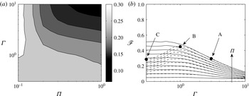
(a) Contour plot of the long-term limit (
 $t^{\prime }=1000$
) of
 $V^{\prime }(t^{\prime })/{\it\Pi}t^{\prime }\rightarrow V_{u}({\it\Gamma},{\it\Pi})$
, see (4.1). (b) The long-time limit (
 $t^{\prime }=1000$
) of the amount of original aquifer fluid compared with the injected fluid that is extracted during an extraction cycle,
 $\mathscr{F}$
, as a function of
 ${\it\Gamma}$
, for
 ${\it\Pi}=0.1$
to
 ${\it\Pi}=1$
in intervals of
 $0.1$
, with a vertical arrow showing the increase in
 ${\it\Pi}$
. The solid (dashed) lines show the numerical results from having an open boundary downslope (upslope) of the extraction well. A, B and C are related to figures 4 and 5.

Profiles of the thickness,
 $F({\it\eta},t^{\prime })$
, as a function of the distance,
 ${\it\eta}$
, in the aquifer during the first and second injection cycles and the first extraction cycle,
 $0\leqslant t^{\prime }\leqslant 3$
, are shown in figure 6(a) at dimensionless times
 $t^{\prime }=0.5$
, 1, 1.5, 2, 2.5 and 3 for
 ${\it\Gamma}=0.5$
and
 ${\it\Pi}=0.4$
. Figure 6(b) shows how the downslope nose,
 ${\it\eta}_{R_{nose}}$
, and the upslope nose,
 ${\it\eta}_{L_{nose}}$
, vary as a function of time,
 $t^{\prime }$
, for
 ${\it\Gamma}=1$
and
 ${\it\Pi}=0.2$
. We see that the downslope nose oscillates as a result of the open boundary downslope of the injection and extraction well.
Figure 6(c) compares the profiles of the current at the end of the injection phases after many cycles are complete, namely at
 $t^{\prime }=9$
, 49 and 99 for
 ${\it\Gamma}=1$
and
 ${\it\Pi}=0.2$
. It may be seen that
 ${\it\eta}_{R_{nose}}(t^{\prime })$
continues to increase with time, indicating how the flow continues to spread downslope into the saturated rock. In figure 6(d) we show the variations of the current thickness
 $F({\it\eta},t^{\prime })$
as a function of position
 ${\it\eta}$
during an injection–extraction cycle at long time (
 $t^{\prime }=998.0$
, 998.5, 999 and 999.5), for
 ${\it\Gamma}=0.5$
and
 ${\it\Pi}=0.4$
.
It may be seen, in figure 6(c,d), that the current organises itself into two regions. Near the source, there is a large-amplitude oscillation in the thickness of the current over each cycle, while beyond this region, the current largely involves a net outward flow associated with the sloping aquifer. We define the height,
 $F_{C}$
, of the net outward flow in (3.1).
At long times the volume of the current increases linearly with time,
 $V(t^{\prime })\sim t^{\prime }$
. For example, in figure 6(e) we show the variation with time of the quantity
 $V^{\prime }(t^{\prime })/{\it\Pi}t^{\prime }$
, at the end of each extraction cycle, for
 ${\it\Gamma}=1$
and
 ${\it\Pi}=0.1$
,
 $0.2$
,
 $0.3$
and 1. In each case
 $V^{\prime }(t^{\prime })/{\it\Pi}t^{\prime }$
becomes independent of time,
 $t^{\prime }$
, at large times, and in general we can define the quantity
 $$\begin{eqnarray}\displaystyle \lim _{t^{\prime }\rightarrow \infty }\frac{V^{\prime }(t^{\prime })}{{\it\Pi}t^{\prime }}=V_{d}({\it\Gamma},{\it\Pi}), & & \displaystyle\end{eqnarray}$$
which is well defined and varies with
 ${\it\Gamma}$
and
 ${\it\Pi}$
.
Profiles of the thickness,
 $F$
, as a function of the distance,
 ${\it\eta}$
, in the aquifer after the 50th injection–extraction cycle,
 $t^{\prime }=99$
, are shown in figure 7 for the combinations of
 ${\it\Gamma}=0.3$
, 1 and 3, and
 ${\it\Pi}=0.1$
and 1. We also show profiles of the current near the injection and extraction well in order to understand the behaviour of the current. By increasing
 ${\it\Pi}$
we can see that more of the injected fluid has moved downslope away from the injection and extraction well. For
 ${\it\Gamma}\gg 1$
we see that a small amount of fluid leaks into the aquifer compared with the case
 ${\it\Gamma}\ll 1$
, because there is no flow through the upper boundary, which leads to the migration of injected fluid away from the well. In contrast to the results of § 3, the amount of fluid leaking into the aquifer increases monotonically as
 ${\it\Gamma}$
decreases, because the pressure driven oscillating flow which dominates when
 ${\it\Gamma}\ll 1$
moves fluid downslope towards the open boundary. These variations of the volume are shown in figure 8(a), where we illustrate a contour plot of
 $V_{d}$
, see (4.1), as a function of
 ${\it\Gamma}$
and
 ${\it\Pi}$
.
Figure 8(b) shows the long-time (
 $t^{\prime }=1000$
) fraction of original aquifer fluid, compared with the injected fluid, that is extracted during an extraction cycle,
 $\mathscr{F}$
(see (2.20)), as a function of
 ${\it\Gamma}$
. Curves are shown for different values of
 ${\it\Pi}$
in the range 0.1–1, in increments of
 $0.1$
. The dashed lines show the corresponding results calculated in § 3 for the case in which the open boundary is upslope of the injection and extraction well. We see that the fraction is always lower when the open boundary is upslope (dashed lines) of the extraction well compared with when the open boundary is downslope (solid lines) of the extraction well.
Using (2.15), the position of the downslope nose of the current, at long time as given by (2.18), is equal to
 $$\begin{eqnarray}x_{R_{nose}}(t)=S\sin ({\it\theta})t+s(t^{\prime })\frac{Q{\it\tau}}{H{\it\phi}},\end{eqnarray}$$
where
 $s(t^{\prime })$
is defined in (3.5). The nose of the current oscillates due to the movement of the injected and original fluid towards and away from the open boundary downslope from the injection extraction well. We do not see this in § 3 as the open boundary is upslope of the injection and extraction well. If the upslope nose of the current has passed the zone of oscillation by a significant distance, then from (2.15) we find
 $$\begin{eqnarray}-x_{L_{nose}}(t)\leqslant HF_{C}\cot ({\it\theta}).\end{eqnarray}$$
This is confirmed numerically in figure 6(b), where
 $F_{C}$
is defined in (3.1).
This downslope far-field solution appears to correspond to a self-similar flow in which there is a constant outward flux of source fluid and inward flux of original reservoir fluid resulting from a fixed height of injected fluid at the injection and extraction well. In § 5 we develop a new family of exchange flow solutions, with zero net flux, and show that this far-field flow asymptotes to these solutions after many cycles.
5. Inclined exchange flow with zero net flux
The numerical solutions presented in §§ 3 and 4 suggest that at long times, the downslope far-field spreading of the injected fluid is self-similar (figures 5 and 8). Since there is no net flow, we now explore whether this corresponds to a family of exchange flows in which the hydrostatic head at the source,
 $h_{0}$
, is the equivalent control parameter to the values of
 ${\it\Gamma}$
and
 ${\it\Pi}$
in the oscillatory flow. We develop these new solutions and test them with a series of further new laboratory experiments. We hypothesise that these correspond to there being a reservoir of dense source fluid with different depths
 $h_{0}$
, where
 $0<h_{0}<H$
.
We consider the migration of fluid of density
 ${\it\rho}+{\rm\Delta}{\it\rho}$
and viscosity
 ${\it\mu}$
into a fully saturated aquifer of depth
 $H$
inclined at an angle
 ${\it\theta}$
to the horizontal, initially filled with fluid of the same viscosity
 ${\it\mu}$
but of density
 ${\it\rho}$
. We assume that the reservoir is filled with a layer of depth
 $h_{0}<H$
of density
 ${\it\rho}+{\rm\Delta}{\it\rho}$
, and the region
 $h_{0}<y\leqslant H$
is filled with fluid of density
 ${\it\rho}$
, as shown in figure 9. As in § 2, we assume that the aquifer has porosity
 ${\it\phi}$
and permeability
 $k$
, and has impermeable upper and lower boundaries. We focus on flows with a small aspect ratio (depth/length)
 $\ll 1$
, in which case the flow is approximately one-dimensional and parallel to the boundary, and the vertical pressure gradient is approximately hydrostatic.
Schematic illustration of fluid, with density
 ${\it\rho}$
and viscosity
 ${\it\mu}$
, in an aquifer, of height
 $H$
, with permeability
 $k$
, porosity
 ${\it\phi}$
and inclined at an angle
 ${\it\theta}$
to the horizontal. We have illustrated both the fluid being injected and extracted at the source and the hydrostatic head height of the current at the source,
 $h_{0}$
. Note that
 $h_{0}$
is constant. The injected fluid has density
 ${\it\rho}+{\rm\Delta}{\it\rho}$
and viscosity
 ${\it\mu}$
, and we show the position of the leading edge,
 $x_{nose}(t)$
, and the height of the intruding fluid,
 $h_{l}(x,t)$
.

5.1. Governing equations
We focus on the region
 $x\geqslant 0$
, and note that the invading current of density
 ${\it\rho}+{\rm\Delta}{\it\rho}$
occupies the region
 $0\leqslant y<h_{l}(x,t)\leqslant h_{0}\leqslant H$
and
 $0\leqslant x\leqslant x_{nose}(t)$
, where
 $$\begin{eqnarray}h_{l}(x_{nose}(t),t)=0\quad \text{and}\quad h_{l}(0,t)=h_{0}.\end{eqnarray}$$
We seek solutions of a flow with a zero net flux, and by using (2.8) with
 ${\it\lambda}=0$
, we obtain the governing equation (see Hesse, Tchelepi & Orr Reference Hesse, Tchelepi and Orr2008)
 $$\begin{eqnarray}\displaystyle \frac{\partial h_{l}}{\partial t}+S\sin ({\it\theta})\frac{\partial }{\partial x}\left(h_{l}\left(1-\frac{h_{l}}{H}\right)\right)=S\cos ({\it\theta})\frac{\partial }{\partial x}\left(\left(1-\frac{h_{l}}{H}\right)h_{l}\frac{\partial h_{l}}{\partial x}\right). & & \displaystyle\end{eqnarray}$$
In order to gain some insight into the long-time behaviour of the system, we neglect the term on the right-hand side in (5.2). We then use the solution to determine when this approximation is self-consistent in (5.10). We can solve the advection equation by defining a similarity variable
 $$\begin{eqnarray}{\it\zeta}=\frac{x}{S\sin ({\it\theta})t}=\frac{{\it\eta}}{{\it\Pi}t^{\prime }},\quad \text{where }h_{l}(x,t)=Hg({\it\zeta}),\end{eqnarray}$$
where
 ${\it\Pi}$
,
 ${\it\eta}$
and
 $t^{\prime }$
are defined in (2.11) and (2.15). The constant depth at the source and the scaled length of the current (5.1) are given by
 $$\begin{eqnarray}G(0,{\it\sigma})=g_{0}=\frac{h_{0}}{H},\quad {\it\chi}_{nose}({\it\sigma})=\frac{x_{nose}(t)}{S\sin ({\it\theta})}.\end{eqnarray}$$
Neglecting the diffusion term, (5.2) reduces to the form
 $$\begin{eqnarray}\displaystyle -{\it\zeta}\frac{\partial g}{\partial {\it\zeta}}+\frac{\partial }{\partial {\it\zeta}}\left(g\left(1-g\right)\right)=0, & & \displaystyle\end{eqnarray}$$
which has the solution (cf. Gunn & Woods Reference Gunn and Woods2011 (4.11),
 $V\rightarrow 1$
)
 $$\begin{eqnarray}g=\left\{\begin{array}{@{}ll@{}}g_{0},\quad & 0<{\it\zeta}\leqslant (1-2g_{0}),\\ \frac{1}{2}(1-{\it\zeta}),\quad & (1-2g_{0})<{\it\zeta}\leqslant 1.\end{array}\right.\end{eqnarray}$$
This solution has a constant flux of injected fluid from the source, calculated as
 $$\begin{eqnarray}Q_{l}=g_{0}(1-g_{0})HS\sin ({\it\theta}).\end{eqnarray}$$
The nose of the current has position
 $$\begin{eqnarray}x_{nose}(t)=S\sin ({\it\theta})t=\frac{Q{\it\tau}}{H{\it\phi}}{\it\Pi}t^{\prime },\end{eqnarray}$$
and the volume of the current is given by
 $$\begin{eqnarray}V_{l}(t)=g_{0}(1-g_{0})HS\sin ({\it\theta})t=Q{\it\tau}g_{0}(1-g_{0}){\it\Pi}t^{\prime }.\end{eqnarray}$$
We can neglect the diffusion term in (5.2) provided that
 $$\begin{eqnarray}\frac{h_{l}}{x}\ll \tan ({\it\theta})\rightarrow t\gg g_{0}\frac{H\cos ({\it\theta})}{S\sin ^{2}({\it\theta})}=\frac{g_{0}{\it\Gamma}^{3}}{{\it\Pi}^{2}}{\it\tau}.\end{eqnarray}$$
This condition is equivalent to (2.18).
5.2. Matching far-field solution
We now compare the downslope far-field solutions that develop from an injection and extraction well with an open boundary either upslope or downslope from the well, described in §§ 3 and 4 respectively, with the exchange flow solutions described above. We hypothesise that the depth of the reservoir,
 $g_{0}$
, in the equivalent exchange flow solutions is given by the height of the outward net flux,
 $F_{C}({\it\Gamma},{\it\Pi})$
, see (3.1), and we now compare the two profiles,
 $g({\it\zeta})$
and
 $F({\it\eta},t^{\prime })$
.
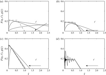
In figure 10 we illustrate the numerical solutions for the oscillatory flow with an open boundary in the upslope direction (§ 3) and the zero net flux exchange flow solutions (§ 5.1) for combinations of
 ${\it\Gamma}=0.3$
and 3 and
 ${\it\Pi}=0.2$
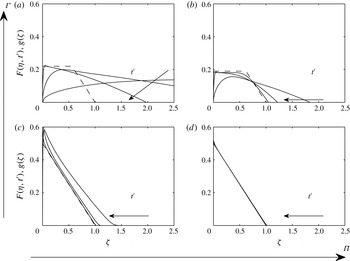
and 1 respectively, illustrating the shape of the flow after 10, 100 and 1000 oscillations in each case. Similarly, in figure 11 we illustrate the numerical solutions for the oscillatory flow with an open boundary in the downslope direction (§ 4) and the zero net flux exchange flow solutions (§ 5.1). This confirms that, in the far field, the long-term oscillatory solution asymptotes to the exchange flow solutions and, therefore, see (3.2) and (4.1),
 $$\begin{eqnarray}V_{u}({\it\Gamma},{\it\Pi})=V_{d}({\it\Gamma},{\it\Pi})=F_{C}(1-F_{C}),\end{eqnarray}$$
where
 $F_{C}$
is the height of the outward net flux, see (3.1). When the advection dominates diffusion, condition (2.18), we find, using (3.2), (4.1) and (5.11), that the volume of the injection and extraction current, §§ 3 and 4, is
 $$\begin{eqnarray}\displaystyle V(t)=F_{C}(1-F_{C})HS\sin ({\it\theta})t. & & \displaystyle\end{eqnarray}$$
Comparison between the asymptotic solution (dashed line) and the full numerical solution from § 3 (solid lines) of the thickness of the fluid front as a function of the scaled position
 ${\it\zeta}$
for combinations of
 ${\it\Gamma}=3$
,
 ${\it\Pi}=0.1$
,
 $g_{0}=0.22$
(a);
 ${\it\Gamma}=3$
,
 ${\it\Pi}=1$
,
 $g_{0}=0.18$
(b);
 ${\it\Gamma}=0.3$
,
 ${\it\Pi}=0.1$
,
 $g_{0}=0.46$
(c);
 ${\it\Gamma}=0.3$
,
 ${\it\Pi}=1$
,
 $g_{0}=0.18$
(d). Numerical solutions are shown at the end of the fifth and 50th extraction cycles, corresponding to times
 $t^{\prime }=10$
, 100 and 1000; the arrows show the direction of time increasing.

Comparison between the asymptotic solution (dashed line) and the full numerical solution from § 4 (solid lines) of the thickness of the fluid front as a function of the scaled position
 ${\it\zeta}$
for combinations of
 ${\it\Gamma}=3$
,
 ${\it\Pi}=0.1$
,
 $g_{0}=0.22$
(a);
 ${\it\Gamma}=3$
,
 ${\it\Pi}=1$
,
 $g_{0}=0.19$
(b);
 ${\it\Gamma}=0.3$
,
 ${\it\Pi}=0.1$
,
 $g_{0}=0.5$
(c);
 ${\it\Gamma}=0.3$
,
 ${\it\Pi}=1$
,
 $g_{0}=0.5$
(d). Numerical solutions are shown at the end of the fifth and 50th extraction cycles, corresponding to times
 $t^{\prime }=10$
, 100 and 1000; the arrows show the direction of time increasing.

We note that the volume,
 $Q{\it\tau}\mathscr{F}$
, of original aquifer that is extracted during an extraction cycle is equal to the net volume of injected fluid that enters the aquifer during the whole injection–extraction cycle. Therefore, we can approximate
 $\mathscr{F}$
as
 $$\begin{eqnarray}\mathscr{F}=2\frac{\partial \bar{V}^{\prime }}{\partial t^{\prime }}=2F_{C}(1-F_{C}){\it\Pi}\leqslant \frac{{\it\Pi}}{2},\end{eqnarray}$$
as
 $F_{C}\leqslant 1/2$
. Here,
 $\mathscr{F}$
, see (2.20), is the long-term limit of the volume of original aquifer fluid as a fraction of the total volume of fluid extracted during one cycle.
6. Contaminants
We have developed a model for the periodic injection and extraction of fluid of one density into an inclined aquifer initially saturated with fluid of a second density as part of a strategy for the inter-seasonal storage of thermal energy in the ground. In such a scheme, it may be that there are contaminants in the original reservoir fluid and it is undesirable to bring these to the surface. Using our model, we now consider the possible transport of such contaminants to the surface. First, in § 6.1, we quantify how the concentration of original aquifer fluid that is extracted evolves with time. Second, in § 6.2, we examine a more complex problem in which there is an initially localised patch of contaminant at some distance from the well, which is drawn to the well after several injection–extraction cycles due to the exchange flow that develops as the tongue of dense injected fluid spreads outwards, see figure 1.
6.1. Concentration of extracted fluid
The concentration of the original aquifer fluid that is extracted during an extraction cycle,
 $C(t^{\prime })$
, can be calculated as the volume fraction,
 $$\begin{eqnarray}C(t^{\prime })=\frac{-[u_{2}H]_{0^{-}}^{0^{+}}}{Q}=1-{\it\Gamma}^{3}\left[F\frac{\partial F}{\partial {\it\eta}}\right]_{0^{-}}^{0^{+}},\end{eqnarray}$$
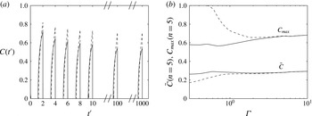
using (2.3)–(2.5). As an example, figure 12(a) shows the variation of
 $C(t^{\prime })$
as a function of time for the case
 ${\it\Gamma}=1$
and
 ${\it\Pi}=0.5$
. The dashed (solid) line uses the model from § 3 (§ 4) and represents an open boundary upslope (downslope) of the extraction well. During each of the first few extraction cycles, it is seen that once the original fluid reaches the extraction well, the concentration of original fluid in the fluid extracted at the well increases to significant values, of order
 ${\sim}60\,\%$
. The extraction of original aquifer fluid begins earlier when the open boundary is upslope of the extraction well (solid), but a higher maximum concentration is achieved when the open boundary is downslope of the extraction well (dashed).
Numerical predictions from the models described in § 4 (§ 3) are shown with a solid (dashed) line. (a) Variation with time of the concentration of original reservoir fluid in the fluid extracted from the aquifer. (b) Variation of the maximum concentration,
 $C_{max}$
, and average concentration,
 $\bar{C}$
, of original reservoir fluid that is extracted from the well on the fifth extraction cycle,
 $n=5$
, as a function of
 ${\it\Gamma}$
for
 ${\it\Pi}=0.5$
.

The maximum concentration during each extraction cycle,
 $$\begin{eqnarray}C_{max}(n)=\max (C(t^{\prime })),\quad \text{when }2n-1<t^{\prime }\leqslant 2n,\end{eqnarray}$$
initially decreases, but then at long time,
 $C_{max}$
asymptotes to a constant value, see figure 12(a). Figure 12(b) shows the variation of the maximum concentration,
 $C_{max}$
, and the average concentration,
 $\bar{C}$
see (2.19), during the fifth extraction cycle,
 $n=5$
, as a function of
 ${\it\Gamma}$
for
 ${\it\Pi}=0.5$
. We see that the maximum concentration is higher when the open boundary is upslope of the extraction well (dashed, § 3) compared with when the open boundary is downslope of the extraction well (solid, § 4). In contrast, the average concentration is lower when the open boundary is upslope of the extraction well (dashed, § 3) compared with when the open boundary is downslope of the extraction well (solid, § 4) which has also been shown in figure 8(b). This is a result of the difference between cooperation of pressure and buoyancy forces and competition between pressure and buoyancy forces which arises either up- or downslope of the well, which becomes significant for small
 ${\it\Gamma}$
. It is worth noting that for small
 ${\it\Gamma}$
and for sufficiently large
 ${\it\Pi}$
, during the extraction cycle there is a period when only original aquifer fluid is extracted,
 $C_{max}=1$
.
6.2. Extraction of distant localised contaminants
In § 6.1, we explored the composition of the produced fluid, showing there may be significant concentrations of original aquifer fluid produced from the well during the extraction cycle. This is important for predicting the potential extraction of contaminants distributed throughout the aquifer. In some situations, there may be localised regions of contaminants in the aquifer (Hunt, Sitar & Udell Reference Hunt, Sitar and Udell1988a ,Reference Hunt, Sitar and Udell b ; Eichel et al. Reference Eichel, Helmig, Neuweiler, Cirpka, Das and Hassanizadeh2005). It is of interest to understand if and when such contaminants are extracted by a periodical injection and extraction system. In §§ 3–5, we demonstrated that, as the injected fluid spreads out, an exchange flow develops in the aquifer downslope of the well, and this leads to a constant return flow of original reservoir water. The injected fluid that migrates upslope from the well, into the aquifer, will also cause a finite amount of original aquifer fluid to be extracted at the well.
We now use the model to calculate the movement of this water as it advances towards the extraction well with time. For simplicity, we only calculate the movement of the original aquifer fluid at the end of the extraction cycle in order to avoid complications due to the oscillating flow. We note that at the end of the extraction cycle, the total amount of original aquifer fluid that has been extracted downslope (upslope) from the extraction well is equal to the total amount of injected fluid that has entered the downslope (upslope) aquifer. Therefore,
 $X_{d}$
(
 $X_{u}$
), defined as the initial position of the fluid originally downslope (upslope) that is extracted at time
 $t$
is given by
 $$\begin{eqnarray}\displaystyle X_{d}^{\prime }(t^{\prime })=X_{d}(t)\frac{H{\it\phi}}{Q{\it\tau}} & = & \displaystyle V_{d}^{\prime }(t)=\int _{0}^{{\it\eta}_{R_{nose}}}F\,\text{d}{\it\eta},\end{eqnarray}$$
 $$\begin{eqnarray}\displaystyle X_{u}^{\prime }(t^{\prime })=X_{u}(t)\frac{H{\it\phi}}{Q{\it\tau}} & = & \displaystyle V_{u}^{\prime }(t)=\int _{{\it\eta}_{L_{nose}}}^{0}F\,\text{d}{\it\eta}.\end{eqnarray}$$
Figure 13(a) shows the variation in the initial dimensionless position of the fluid downslope,
 $X_{d}^{\prime }$
, and upslope,
 $X_{u}^{\prime }$
, of the well that is extracted, as a function of time
 $t^{\prime }$
for
 ${\it\Gamma}=0.8$
and
 ${\it\Pi}=0.2$
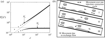
. We see that
 $X_{d}^{\prime }$
increases linearly with time and
 $X_{u}^{\prime }$
asymptotes to a constant value. This means that any original aquifer fluid downslope of the well will eventually be extracted, but only a finite amount of original aquifer upslope of the well will be extracted. This is illustrated schematically in figure 13(b), where the contaminant downslope of the well is drawn towards the well by the exchange flow and the contaminant upslope of the well is initially sufficiently far from the well, see (6.6), and is not extracted.
(a) Variation of the dimensionless distances
 $X_{u}^{\prime }$
and
 $X_{d}^{\prime }$
from the source of the initial position of the original aquifer, see (6.3) and (6.4), which are extracted at time
 $t^{\prime }$
for
 ${\it\Gamma}=0.8$
and
 ${\it\Pi}=0.2$
. Numerical predictions, calculated at the end of the extraction cycle, of an open boundary upslope of the well, § 3, are shown with filled-in circles and theoretical limits are shown with dashed lines, see (6.5) and (6.6). (b) Illustration of the movement of a distant localised contaminant (wavy region) due to the periodic motion (double-headed arrows) and the exchange flow (single-headed arrows). The injected fluid, shaded grey, is shown at the end of the extraction phase, and time increases from I to II to III.

At long time, using (5.12) and (2.15), we can find that
 $$\begin{eqnarray}\displaystyle \lim _{t^{\prime }\rightarrow \infty }X_{d}^{\prime }(t^{\prime }) & = & \displaystyle F_{C}(1-F_{C}){\it\Pi}t^{\prime }=F_{C}(1-F_{C}){\it\eta}_{R_{nose}}(t^{\prime }),\end{eqnarray}$$
 $$\begin{eqnarray}\displaystyle \lim _{t^{\prime }\rightarrow \infty }X_{u}^{\prime }(t^{\prime }) & {\leqslant} & \displaystyle \frac{F_{C}^{2}{\it\Gamma}^{3}}{2{\it\Pi}}=F_{C}\frac{{\it\eta}_{L_{nose}}(t^{\prime })}{2},\end{eqnarray}$$
7. Experiments
We carried out a series of experiments to provide some real data with which to compare our theoretical predictions presented in §§ 3–5.
We used a Hele-Shaw cell that was 1 m long,
 $10$
cm high and had a gap width of
 $d=1$
mm. The injected dense fluid was dyed red to aid visualisation, and photographs were taken and digitally analysed to calculate the profile of the fluid at different times in the experiment. In the Hele-Shaw cell, we observed a small amount of intermingling and possible mixing at the interface between the two fluids, although due to the density stratification the interface appeared to remain quite localised and well defined during the experiments. Indeed, by the end of the experiment, the mixed region, which could be detected as a region of intermediate dye intensity, appeared to be less than 1 cm in thickness (cf. Woods & Mason Reference Woods and Mason2000). We also note that the cross-cell diffusion time scale,
 $d^{2}/D\sim 10^{3}$
s, where
 $D$
is the molecular diffusivity, was considerably longer than the period of each cycle in our experiments, thus limiting the mixing during each cycle, although we would expect a gradual growth of the mixing zone with successive cycles.
In experiments 1 and 2 we injected dense salty water into a tank filled with fresh water. In experiment 3 the dense fluid entering from the reservoir into the Hele-Shaw cell was a mixture of 50 % glycerol and 50 % salty water (9 % salt), and the fluid originally in the tank was 50 % glycerol and 50 % water.
In order to compare the experimental measurements with our model, given an injection rate, we require a value for the parameter
 $S=k{\rm\Delta}{\it\rho}g/{\it\mu}{\it\phi}$
. In experiment 1, the temperature was 20 °C and we found that the density contrast between the aqueous solution and the fresh water was
 ${\rm\Delta}{\it\rho}\sim 40~\text{kg}~\text{m}^{-3}$
, while the fluid viscosity was
 ${\it\mu}\sim 10^{-3}$
Pa s (see Lide Reference Lide2001). The effective permeability of the Hele-Shaw cell was
 $k=d^{2}/12$
, leading to the estimate
 $S\sim 0.033$
m s
 $^{-1}$
. During our experiments, the laboratory temperature varied from 18 to 22 °C, leading to a range in the viscosity from
 ${\sim}0.96\times 10^{-3}$
to
 ${\sim}1.06\times 10^{-3}$
Pa s (linearly interpolating values from Lide Reference Lide2001), resulting in a variation in
 $S$
from
 $0.031$
to
 $0.34~\text{m}~\text{s}^{-1}$
. However, for the present calculations, we neglect such effects and use the value corresponding to 20 °C. The parameter
 $S$
was calculated similarly for experiments 2 and 3, and the viscosity for 50 % water and 50 % glycerol was taken as
 ${\it\mu}\sim 8.4\times 10^{-3}$
Pa s (see Lide Reference Lide2001).
7.1. Injection and extraction experiments
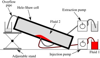
We tested the theory from § 3 by using the experimental set-up shown in figure 14. The downslope far end of the Hele-Shaw cell was sealed, but the upslope far end of the Hele-Shaw cell was open and connected to an open reservoir to accommodate the fluid associated with the inflow and outflow cycles. We pumped the fluid into and out of a hole in the base of the tank, and for each experiment we switched between injection and extraction cycles either every
 $10$
s or every 15 s (
 ${\it\tau}=10$
or 15 s). We also tested the theory from § 4 by using an experimental set-up similar to figure 14 but with the overflow pipe located at the downslope end of the tank. The upslope far end of the Hele-Shaw cell was sealed, but the downslope far end of the Hele-Shaw cell was open and connected to an open reservoir.
Illustration of the experimental set-up showing the inclined Hele-Shaw Cell, the injection and extraction pumps and the overflow pipe.

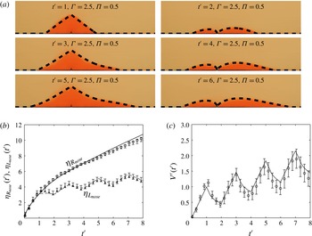
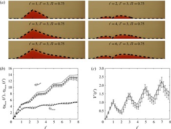
Figures 15(a) and 16(a) each show six photographs of an experiment illustrating the shape of the current after the first, second and third injection and extraction cycles,
 $t^{\prime }=1$
to
 $t^{\prime }=6$
in intervals of 1, and we superimpose the model predictions from § 3 (§ 4) with a dashed line for
 ${\it\Gamma}=2.5$
(3) and
 ${\it\Pi}=0.5$
(0.75) onto the photographs.
Comparison of experimental measurements and the numerical predictions from § 3 of the thickness of the current,
 $F({\it\eta},t^{\prime })$
, as a function of the position,
 ${\it\eta}$
. For this experiment,
 $S=3.3\times 10^{-2}~\text{m}~\text{s}^{-1}$
,
 $Q=4\times 10^{-4}~\text{m}^{2}~\text{s}^{-1}$
,
 ${\it\tau}=10$
s,
 ${\it\theta}=3.5^{\circ }$
. (a) Photographs of the experiment showing the bottom half of the Hele-Shaw cell with numerical predictions superimposed as dashed lines on top. (b,c) Numerical predictions of the current (solid line) and experimental results with error bars. The error bars represent 10 % and 90 % relative changes in light intensity. (b) Position of
 ${\it\eta}_{R_{nose}}$
and
 ${\it\eta}_{L_{nose}}$
and (c) volume of the gravity current as functions of time
 $t^{\prime }$
as predicted by the theoretical model and as measured in the experiments.

Comparison of experimental measurements and the numerical predictions from § 4 of the thickness of the current,
 $F({\it\eta},t^{\prime })$
, as a function of the position,
 ${\it\eta}$
. For this experiment,
 $S=4.5\times 10^{-2}~\text{m}~\text{s}^{-1}$
,
 $Q=3\times 10^{-4}~\text{m}^{2}~\text{s}^{-1}$
,
 ${\it\tau}=15$
s,
 ${\it\theta}=3^{\circ }$
. (a) Photographs of the experiment showing the bottom half of the Hele-Shaw cell with numerical predictions superimposed as dashed lines on top. (b,c) Numerical predictions of the current (solid line) and experimental results with error bars. The error bars represent 10 % and 90 % relative changes in light intensity. (b) Position of
 ${\it\eta}_{R_{nose}}$
and
 ${\it\eta}_{L_{nose}}$
and (c) volume of the gravity current as functions of time
 $t^{\prime }$
as predicted by the theoretical model and as measured in the experiments.

In figures 15(b) and 15(c) (figures 16 b and 16 c) we compare the upslope and downslope positions of the nose of the current and the volume of the current as measured by our experiment, shown as symbols, and as predicted by the model in § 3 (§ 4), shown as solid lines. The error bars represent the points where there are 10 % and 90 % changes in light intensity relative to the difference in light intensity between the upper-layer fluid and the lower-layer fluid. There is a small mismatch in the predicted position of the downslope nose in figure 15(b) (figure 16 b) possibly due to the no-slip condition at the base of the tank (see Neufeld, Vella & Huppert Reference Neufeld, Vella and Huppert2009) or the inter-fluid stress (Woods & Mason Reference Woods and Mason2000). However, the upslope nose, figure 15(b) (figure 16 b), and volume, figure 15(c) (figure 16 c), of the gravity current agree well with the experimental data over the first four injection–extraction cycles.
7.2. Inclined exchange flow experiments
We now test the theory from § 5 by using the experimental set-up shown in figure 17(a). The end of the tank is attached to a reservoir of fluid with a lock gate and the other end of the tank is sealed so that at all times there is zero net volume flow rate in the Hele-Shaw cell.
(a) Photograph and labels of the experimental set-up. The Hele-Shaw cell is connected to a large reservoir through a lock gate. The reservoir is set up with two layers of fluid. Fluid 1, dyed red, is 50 % glycerol and 50 % salty water (4.5 % salt), and fluid 2 is 50 % glycerol and 50 % water. The tank is inclined at an angle of
 ${\it\theta}$
to the horizontal, which can be altered using the adjustable stand. (b,c) Comparison of experimental measurements and numerical predictions of the thickness of the current,
 $G({\it\zeta})$
, as a function of the position,
 ${\it\zeta}$
. (b) Two photographs compared with the theoretical predictions (dashed lines) at times
 $t=6$
s and
 $t=14$
s. For this experiment the tank was inclined at
 $35^{\circ }$
,
 $S=3\times 10^{-2}~\text{m}~\text{s}^{-1}$
,
 $H=0.1$
m and the source height is
 $h_{0}=H\times 0.37$
m. (c) Numerical predictions of the current (solid line) and the experimental results with error bars; the error bars represent the maximum and minimum thickness of the fluid at position
 ${\it\zeta}$
for times
 $t=3$
s to
 $t=20$
s in intervals of 1 s.

We carefully created a two-layered system in the reservoir with a mixture of 50 % glycerol and 50 % aqueous saline solution (4.5 % salt) placed below the reference mixture of 50 % glycerol and 50 % water. Experiments were carried out for a range of values of the thickness of the lower relatively dense layer,
 $g_{0}$
. Before each experiment, the Hele-Shaw cell was filled with the reference fluid. To start each experiment, the lock gate was opened and fluid in the reservoir exchanged with the fluid in the Hele-Shaw cell. Two photographs, figure 17(b), show the shape of the current at the times
 $t=6$
s and
 $14$
s for
 $g_{0}=0.37$
. The numerical models are in good agreement with the experiment. The shape of the current as a function of
 ${\it\zeta}$
was measured at a series of times,
 $t=3$
s to
 $t=20$
s in time steps of 1 s. In figure 17(c), we show measurements of the thickness of the current at a series of values of the dimensionless position
 ${\it\zeta}$
, and averaged over the measurements at the different times, from experiment 3. The error bars, which are very small, illustrate the variation of the value of
 $g$
at each dimensionless point
 ${\it\zeta}$
between the 18 times, suggesting that the self-similar solution provides a good model of the flow (the sum of the area between the experimental current profile and the theoretical prediction is less than 1 % of the total area).
8. Conclusion
In this paper we have explored the periodic injection and extraction of fluid from a permeable inclined aquifer of finite vertical extent. This problem has relevance for inter-seasonal thermal energy storage schemes in which excess thermal energy produced in the summer can be stored underground for recovery in the winter. Using the model we have calculated the concentration and quantity of contaminants in the extracted fluid that were originally in the aquifer, see figures 1 and 13(b).
This paper focuses on the role of density differences between the injected and reservoir fluids in controlling the dispersion of the fluid injected into the aquifer, and in order to quantify these effects we have developed a two-layer model for the combined pressure driven and gravity driven flow of the injected and original reservoir water. The model strictly applies during the few cycles before dispersive effects are significant, see § 1, but for interest we show results up to
 $t^{\prime }=1000$
.
We have considered two cases in which there is an open boundary either upslope (§ 3) or downslope (§ 4) of the source, with the other boundary being sealed. In both cases we find that, although initially the amount of injected fluid recovered increases, a constant amount of injected fluid is not recovered during each injection–extraction cycle. The fraction that is not recovered depends on
 ${\it\Gamma}=H(S\cos ({\it\theta}){\it\phi}^{2}/{\it\tau}Q^{2})^{1/3}$
and
 ${\it\Pi}=HS\sin ({\it\theta}){\it\phi}/Q$
. As
 ${\it\Pi}$
decreases, more of the injected fluid is recovered during extraction. Given a constant
 ${\it\Gamma}$
and
 ${\it\Pi}$
, we find that when there is an open boundary downslope (§ 4), more of the original aquifer fluid is extracted compared with when there is an open boundary upslope (§ 3) of the injection and extraction well. We have shown that the leakage flux asymptotes to a family of zero net flux exchange flow solutions which develop when a reservoir containing a fixed thickness of dense fluid is connected to the inclined aquifer, § 5. In § 6 we have investigated how the concentration of original aquifer fluid in the extracted fluid varies with time, and we have explored the time taken for distant undesirable fluids, downslope of the extraction well, to be extracted due to the zero net flux exchange flow. However, upslope of the extraction well only a finite amount of original aquifer fluid is extracted. We have tested our model predictions with a series of new experiments using a Hele-Shaw cell in § 7 and obtained good agreement.
As a simple application of this model, let us consider the injection of water (
 ${\it\mu}=10^{-3}~\text{m}^{2}~\text{s}^{-1}$
) for half a year (
 ${\it\tau}=1.5\times 10^{7}$
s) along a 1 km horizontal well with an injection rate of
 $10^{-2}~\text{m}^{3}~\text{s}^{-1}$
(
 $Q=10^{-5}~\text{m}^{2}~\text{s}^{-1}$
), with a density contrast,
 ${\rm\Delta}{\it\rho}$
, of
 $100~\text{kg}~\text{m}^{-3}$
, into an aquifer of permeability
 $k=10^{-12}~\text{m}^{2}$
, vertical extent
 $H=20$
m, inclined at an angle of
 $5^{\circ }$
to the horizontal, and porosity
 ${\it\phi}=0.1$
, with an open boundary upslope of the injection and extraction well. This leads to the values
 ${\it\Gamma}=0.8$
and
 ${\it\Pi}=0.2$
. We find that after 10 (100) years the leading edge of the injected fluid has moved 500 (4000) m downslope and a maximum of 200 (250) m upslope from the well. We find that the maximum concentration of original aquifer fluid that is extracted during the last extraction cycle is 0.54 (0.46) %. We also find that the volume of the injected current is
 $2.5\times 10^{5}$
 $(1.5\times 10^{6})~\text{m}^{3}$
and that all the aquifer fluid within a distance of 100 (800) m downslope and 15 (20) m upslope from the well has been extracted.
It would be interesting to develop the model further by including open boundaries upslope and downslope of the well, resulting in a net flux moving both upslope and downslope. It would also be interesting to assess the impact of effects associated with mechanical dispersion (Gelhar, Welty & Rehfeldt Reference Gelhar, Welty and Rehfeldt1992; Szulczewski & Juanes Reference Szulczewski and Juanes2013; Woods Reference Woods2015) and the effects associated with heterogeneity and layering of a porous rock (Neufeld & Huppert Reference Neufeld and Huppert2009; Farcas & Woods Reference Farcas and Woods2015; Woods Reference Woods2015). Furthermore, it would be useful to investigate the effects associated with gravity segregation on the heat transfer within permeable rock (Gringarten & Sauty Reference Gringarten and Sauty1975; Dudfield & Woods Reference Dudfield and Woods2012).
Acknowledgements
We thank the three referees of this paper for their valuable comments on an earlier draft.