





1 Introduction
Many engineering applications, including intelligent transportation systems, logistics, smart vehicles, and pickup-and-delivery services, require solving complex routing problems. These problems involve a vehicle or fleet of vehicles reaching a set of destinations while minimizing travel distance to save time, money, energy, and, in some cases, reduce pollution.
Although each application has its own peculiarities, the problem formulation shares an omnipresent core, named in the literature the Traveling Salesperson Problem (TSP); the name comes from the problem’s most famous formulation: “A salesman has to visit a set of cities, each of which must be visited only once, and he wants to minimize the length of the tour.” More formally, given a weighted graph, the TSP requires to compute the minimum cost cycle that visits each vertex exactly once.
Most routing problems are intractable, typically NP-hard. While heuristic approaches can quickly provide good solutions in some cases, systematic algorithms are preferred in others. These algorithms can find the optimal solution, complete with a proof of optimality (in the eXplainable AI spirit) given enough time. Clearly, obtaining the provably optimal solution adds significant value.
The basic TSP problem attracted the attention of researchers in different research areas, including operations research and artificial intelligence, with solution methods ranging from Integer Linear Programming, to Constraint Programming, to metaheuristics, just to name a few (Caseau and Koppstein Reference Caseau and Koppstein1993; Aguiar-Melgarejo et al. Reference Aguiar-Melgarejo, Laborie and Solnon2015; Ducomman et al. Reference Ducomman, Cambazard and Penz2016; Boudreault and Quimper Reference Boudreault and Quimper2021). Beside the basic TSP problem, engineering applications involve a series of other requirements; the need to take into account such requirements spawned a plethora of extensions to the TSP, for example requiring each node to be visited in a time window (TSP with time windows), assuming that more than one agent (or vehicle) is available (Multiple TSP), or that not all nodes must be visited. For example, in the Generalized Traveling Salesperson Problem (GTSP) (Laporte and Nobert Reference Laporte and Nobert1983; Laporte et al. Reference Laporte, Mercure and Nobert1987) (also known as set TSP) the nodes of the graph are partitioned into various sets, called clusters; an optimal solution of the GTSP is a minimum cost cycle that visits at least one node in each cluster. The GTSP models situations in which it is necessary to collect resources in an environment where several equivalent providers are available for each resource type, while minimizing travel time, or energy requirements from a battery.
In the theoretical formulation of the TSP, the weights on the arcs can take any positive value without restrictions; however in most practical cases it is reasonable to assume that the distance function obeys the triangular inequality, where going directly from a node
 $A$
to a node
 $B$
cannot be more expensive than taking a detour to a third node
 $C$
: such case is named metric TSP in the literature. Even more, in many industrial applications, the nodes are associated to points in the plane, they are connected through straight lines, and the distance is the length of the segment connecting the two nodes; this case is named the Euclidean Traveling Salesperson Problem (ETSP), and many instances in the TSPLIB (Reinelt Reference Reinelt1991) set of benchmarks fall in this category. The techniques proposed in this paper are intended for complete Euclidean instances. They do not cover routing settings in which crossings are unavoidable, or in which replacing crossing connections with uncrossed ones would produce infeasible links, as may occur in real road networks. Such settings are outside the scope of the present work.
From the computational complexity point of view, both the metric and the Euclidean TSP are NP-hard (Garey et al. Reference Garey, Graham and Johnson1976), even though, differently from the general TSP, the Euclidean TSP admits a Polynomial Time Approximation Scheme (PTAS) (Arora Reference Arora1996; Mitchell Reference Mitchell1999).
Currently, the best solver for the TSP is the mathematical programming solver Concorde (Applegate et al. Reference Applegate, Bixby, Chvátal and Cook2001). Concorde is based on Integer Linear Programming (ILP) techniques such as branch-and-cut and it was used to optimally solve instances with tens of thousands of nodes. However, most of the algorithms developed for solving the TSP, including Concorde, can only be used when addressing the basic TSP, whereas when there are other additional constraints, it becomes necessary to adopt more general solving techniques.
A general technique developed in Artificial Intelligence to solve Constraint Optimization Problem (COPs) is constraint propagation (Mackworth Reference Mackworth1977). The idea was so successful that new languages were embedding it as part of their operational semantics; for example the Constraint Logic Programming (CLP) (Jaffar and Maher Reference Jaffar and Maher1994) class of languages was defined to declaratively address constraint problems, and many languages of this class exploited constraint propagation to efficiently solve constraint problems. The CLP research area was later extended to include also imperative and object-oriented programming languages, generating the Constraint Programming (CP) research area.
In CP, programmers can easily define constraint optimization problems, including side constraints, without being limited to linear or convex constraints or objective functions. This flexibility makes CP ideal for solving industrial optimization problems. Over the years, numerous solvers have been developed, and today, a variety of open-source and commercial solvers are available and widely used in both academic and commercial applications.
Many works in the CP literature address the TSP (Caseau and Laburthe Reference Caseau and Laburthe1997; Kaya and Hooker Reference Kaya and Hooker2006; Benchimol et al. Reference Benchimol, van Hoeve, Régin, Rousseau and Rueher2012; Fages and Lorca Reference Fages and Lorca2012; Fages et al. Reference Fages, Lorca and Rousseau2016; Deudon et al. Reference Deudon, Cournut, Lacoste, Adulyasak and Rousseau2018); the usual way to tackle Euclidean TSPs is to compute the distance matrix and address the problem as a general TSP. On the other hand, this approach disregards all the additional information available in the ETSP: the coordinates of the points to be visited are known, and geometrical concepts (straight line segments, angles, etc.) can be defined in the Euclidean plane. An interesting research question is: “Is it possible to exploit the additional information intrinsically available in Euclidean instances in order to speed up the search?” An initial answer was presented in a conference publication by Bertagnon and Gavanelli (Reference Bertagnon and Gavanelli2020), where a significant speedup was obtained in solving Euclidean instances in CLP, by exploiting efficient constraint propagation algorithms tailored for Euclidean TSP instances. This article significantly extends that work (Bertagnon and Gavanelli Reference Bertagnon and Gavanelli2020), providing deeper insights, comprehensive analysis, and additional findings.
As a first contribution, we provide a more precise description of the introduced algorithms and we extend the experimental campaign by testing the proposed algorithms on a large dataset of TSP instances, including publicly available and synthetic instances.
Now, a further research question could be whether such enhanced pruning can also be applied beyond the TSP: as a second contribution, this article shows that the additional pruning based on geometric properties is not confined only to the case of the Euclidean TSP, but can also be applied to other variants of routing problems. For instance, we show how the proposed techniques can be applied to the Euclidean Generalized Traveling Salesperson Problem (EGTSP).
The underlying no-crossing and convex-hull ordering properties are classical geometric results; our contribution lies in translating them into dedicated CP/CLP constraints and propagators, and in extending this approach to the EGTSP.
We believe that this work could inspire researchers to extend the devised algorithms also to other routing problems, and also to inspire new propagation algorithms to exploit the additional information present in geometric instances deeply.
The rest of the article is organized as follows. In Section 2 we introduce the necessary definitions and notations. In Section 3 we discuss related works. In Section 4 we provide a description of our techniques that can exploit the geometric information present in the ETSP to improve propagation. In Section 5 we show how geometric information can also be exploited in other variants of routing problems; we take EGTSP as an example. We show the computational results in Section 6 and, finally, in Section 7 we conclude.
2 Preliminaries and notation
A Constraint Satisfaction Problem (CSP) is a triple
 ${\mathscr{P}} = \langle \mathcal{X},\mathcal{D},\mathcal{C} \rangle$
where
 $\mathcal{X}$
is a set of
 $n$
decision variables
 $\lbrace x_{1}, x_{2}, \ldots , x_{n} \rbrace$
,
 $\mathcal{D}$
is a set of domains
 $\lbrace {Dom(x_1)}, {Dom(x_2)},\ldots , {Dom(x_n)}\rbrace$
and
 $\mathcal{C}$
is a set of constraints
 $\lbrace c_{1}, c_{2}, \ldots , c_{m} \rbrace$
. Each domain
 $Dom(x_i)$
is the set of all possible values that can be assigned to the variable
 $x_{i}$
. Each constraint
 $c_{i}$
consists of a pair
 $\langle R_{i}, S_{i} \rangle$
where
 $R_{i}$
is a relation between the variables
 $S_{i}$
participating in the constraint.
A solution for a CSP
 $\mathscr{P}$
is an instantiation that assigns a value to each variable in
 $\mathcal{X}$
and satisfies all the constraints
 $\mathcal{C}$
. While in a CSP all solutions are equally good, in many practical cases an objective function discriminates between solutions.
A Constraint Optimization Problem (COP) is a pair
 $\langle {\mathscr{P}},f \rangle$
where
 ${\mathscr{P}} = \langle \mathcal{X},\mathcal{D},\mathcal{C} \rangle$
is a CSP and
 $f$
a function
 $f : {Dom(x_{1})} \times \ldots \times {Dom(x_{n})} \rightarrow \mathbb{R}$
that associates a value to every solution of
 $\mathscr{P}$
. A solution
 $s$
of
 $\mathscr{P}$
is an optimal solution of the COP
 $\langle {\mathscr{P}},f \rangle$
if and only if there is no solution
 $s'$
of
 $\mathscr{P}$
such that
 $f(s') \lt f(s)$
.
In order to speed up the search of solutions, constraint programming systems alternate search with constraint propagation; each constraint is implemented by a collection of propagators. Each propagator’s objective is to observe the domains of the variables involved in the constraint and, as soon as a value is removed from the domain of a variable, it checks if some values from other domains have become unsupported and can be removed (pruned).
A propagator that is selected for execution is said to be awakened, or activated. The execution of a propagator can have one of three possible outcomes. In the first case, the propagator realizes that the constraint has no solution, for example because a domain becomes empty as a result of deleting some values. In this case a failure is returned and the search algorithm undoes the last choice(s) and attempts different assignments.
In the second case, the propagator finds that the constraint is entailed, that is, it is satisfied whatever the values assumed by the variables among those remaining in the domains. In this case, the propagator can be deallocated.
In the third case, neither of the previous two cases has occurred and so the propagator at the end of the execution is suspended waiting for an event to occur.
The TSP is defined on a weighted graph
 $G=(V,E,w)$
, where
 $V$
is a set of nodes (
 $\vert V \vert = {n}$
),
 $E$
is a set of edges, and
 $w : E \mapsto \mathbb{R}^+$
. A path in
 $G$
is a sequence
 ${{{p}}_{v_{{s}_0}-v_{{s}_k}}} = v_{{s}_0} e_{{s}_0,{s}_1} v_{{s}_1} \ldots e_{{s}_{k-1},{s}_k} v_{{s}_k}$
such that:
-
(i)
 $v_{{s}_0} , v_{{s}_1} , \ldots , v_{{s}_k} \in V$
and are all distinct, and
-
(ii)
$e_{{s}_0,{s}_1} , e_{{s}_1,{s}_2} , \ldots , e_{{s}_{k-1},{s}_k} \in E$
.


Since a path is uniquely identified by the sequence of its nodes (or of its edges) in the proper order, we will often write paths as sequences of nodes to simplify the notation. The length of a path p is the sum of the weights of its edges:
 ${L({p})} = \sum _{i=0}^{k-1} w(e_{s_i,s_{i+1}})$
. A circuit c is a sequence obtained by appending
 $e_{{s}_k,{s}_0}$
to a path
 ${{p}}_{v_{{s}_0}-v_{{s}_k}}$
. A circuit that visits each vertex exactly once is often referred as Hamiltonian circuit.
In the Euclidean case, let
 ${\mathcal {P}}=\{{P}_1,\ldots ,{P}_n\}$
be a set of points, where
 ${P}_i=(x_i,y_i)$
. The graph associated with
 $\mathcal {P}$
is
 $G^{\mathcal {P}} = ({\mathcal {P}},E^{\mathcal {P}},w^{\mathcal {P}})$
, where
 $E^{\mathcal {P}}=\{e_{i,j} \equiv ({P}_i,{P}_j)\mid {P}_i,{P}_j \in {\mathcal {P}}, i\neq j\}$
and
 $w({P}_i,{P}_j)= {d({P}_i,{P}_j)}$
, where
 $d$
is the Euclidean distance.
We use
 $\overline {{P}_i {P}_j}$
to denote the segment in the plane with the extremes
 ${P}_i$
and
 ${P}_j$
. Since in the Euclidean case every edge of a graph corresponds to a segment in the plane between the corresponding endpoints, we will often confuse the edge
 $e_{i, j}$
with the corresponding segment
 $\overline {{P}_i {P}_j}$
. Also, we will sometimes confuse the index
 $i \in V$
with the corresponding point
 ${P}_i$
in the plane. We denote with
 $\overleftrightarrow {{P}_i {P}_j}$
the (infinite straight) line passing through points
 ${P}_i$
and
 ${P}_j$
, and with
 $\angle {P}_i{P}_j{P}_k$
the counter-clockwise angle formed by the segments
 $\overline {{P}_i {P}_j}$
and
 $\overline {{P}_j {P}_k}$
with vertex in
 ${P}_j$
from
 ${P}_i$
to
 ${P}_k$
.
A crossing in a path p is defined as a common point
 ${P}_q \notin {\mathcal {P}}$
(i.e., internal to two edges) that is shared by two (or more) edges of p or a common point
 ${P}_r \in {\mathcal {P}}$
(i.e. an endpoint of some edge) that is shared by three (or more) edges of
 $p$
.
In the CP literature, three main representations have been devised for modeling the Hamiltonian circuit problem and the TSP: the permutation representation, the successor representation, and the set variable representation (Benchimol et al. Reference Benchimol, van Hoeve, Régin, Rousseau and Rueher2012). The last was also extended to the graph representation (Dooms et al. Reference Dooms, Deville and Dupont2005; Fages and Lorca Reference Fages and Lorca2012; Fages et al. Reference Fages, Lorca and Rousseau2016).
In the permutation representation, n variables
 $Pos_{i}$
are introduced
 $ Pos = (Pos_1, Pos_2, \ldots , Pos_{n})$
each with initial domain
 $V$
; variable
 $Pos_{i}$
represents the
 $i$
-th node that is visited. For example, if
 ${n} = 5$
and
 $Pos = (3,5,4,2,1)$
the corresponding tour will be
 $(3,5,4,2,1,3)$
. The constraint model for the permutation representation includes an alldifferent
 $(Pos)$
constraint (Régin Reference Régin1994) on the
 $Pos$
array of variables, that ensures that each node is visited only once.
The set variable representation is based on a set variable (Puget Reference Puget1992; Gervet Reference Gervet1993) that represents the edges that form the tour.
In the successor representation, n variables
 ${\text{ Next}}_i$
are defined
 $ {\text{ Next}} = ({\text{ Next}}_1, {\text{ Next}}_2, \ldots , {\text{ Next}}_{n})$
; variable
 ${\text{ Next}}_i$
represents the node that follows node
 $i$
in the circuit, and its initial domain is
 $\{1,\ldots ,{n}\} \setminus \{i\}$
. For example, if
 ${n} = 5$
and
 ${\text{ Next}} = (3,5,4,2,1)$
the corresponding tour will be
 $(1,3,4,2,5,1)$
.
The constraint model of the successor representation includes, as in the permutation representation, an
 ${\tt alldifferent}({\text{ Next}})$
constraint on the
 $\text{ Next}$
array of variables, that in this case ensures that each node has exactly one incoming edge (degree constraints). The constraint model for the successor representation also includes a circuit
 $({\text{ Next}})$
(Beldiceanu and Contejean Reference Beldiceanu and Contejean1994; Caseau and Laburthe Reference Caseau and Laburthe1997; Kaya and Hooker Reference Kaya and Hooker2006) constraint (sometimes called nocycle) that avoids subtours, that is, cycles of length less than n (subtour-elimination constraints).
In some cases, the constraint model includes, as redundant representation, also a set of
 $\text{ Prev}$
variables:
 ${\text{ Prev}}_i$
represents the node that precedes node
 $i$
in the circuit. Often, constraint models include redundant representations to obtain additional pruning.
Both the alldifferentand the circuit constraints are already implemented in most constraint logic programming systems. Hereafter, unless otherwise specified, we refer always to the successor representation.
3 Related work
As already introduced, the Traveling Salesperson Problem is probably one of the most studied COP in the scientific literature. Many approaches proposed for its resolution have been published over time, even if we limit ourselves only to the Constraint Programming literature. Usually, when it comes to exploit the objective function to prune the search space, CP formulations are not as effective as Integer Programming models, but they are more flexible in dealing with side constraints. To date in the CP literature, the most efficient solving methods are those that combine constraint propagation with ILP techniques. These hybrid methods yield the solving performance of CP models, under certain conditions, comparable to that obtained by ILP models.
Various works propose to use relaxations of the TSP to prune suboptimal branches; the classical relaxations of the TSP are the assignment problem and the one-tree relaxation. Caseau and Laburthe (Reference Caseau and Laburthe1997) propose a simple and effective rule for the circuit constraint (called nocycle). The rule consists in finding a path of mandatory edges of length at most
 $n - 1$
and removing the edge between the two endpoints of the path. They also propose to filter values based on the objective function, using the assignment-based and the spanning tree relaxations.
Kaya and Hooker (Reference Kaya and Hooker2006) propose a new filtering rule based on separator graph, able to remove nonhamiltonian edges, for the circuit constraint.
Francis and Stuckey (Reference Francis and Stuckey2014) consider various propagation algorithms for circuit and provide for each so-called explanations in the context of a lazy clause generation solver.
Fages and Lorca (Reference Fages and Lorca2012) show how properties of the reduced graphs (obtained by introducing a node for each Strongly Connected Component (SCC) of the original graphs) associated to Asymmetric TSPs can be used to improve the Minimum Spanning Tree (MST) relaxation.
Pesant et al. (Reference Pesant, Gendreau, Potvin and Rousseau1998) address the TSP with Time Windows (TSPTW) and exploit the circuit constraint together with the MST relaxation. Focacci et al. (Reference Focacci, Lodi and Milano2002a, Reference Focacci, Lodi and Milano2002b) propose a filtering based on reduced costs for optimization constraints, and in particular use the assignment problem and the minimum spanning forest relaxation.
The groundbreaking work in this area is that by Benchimol et al. (Reference Benchimol, van Hoeve, Régin, Rousseau and Rueher2012): it is the first in which a CP model was able to solve large TSP instances. In their work, they use a variety of techniques. They propose an implementation of the weighted circuit constraint that includes the Held and Karp (Reference Held and Karp1970) scheme, iterates a Lagrangian relaxation to obtain a high-quality one-tree, and uses it to remove edges similarly to reduced costs filtering. It also identifies as mandatory those edges that, if removed, would increase the current lower bound over the quality of the incumbent solution. To find quickly a solution, they first run the Lin-Kernighan-Helsgaun algorithm (Lin and Kernighan Reference Lin and Kernighan1973; Helsgaun Reference Helsgaun2000). In the experiments with asymmetric TSPs, they also use additive bounding (Fischetti and Toth Reference Fischetti and Toth1992) to combine both the 1-tree and the assignment problem relaxations.
In Fages et al. (Reference Fages, Lorca and Rousseau2016), the authors further improve by casting the problem in CP(Graph) and by means of improved search heuristics (i.e., Last Conflict heuristic).
More recently, Boudreault and Quimper (Reference Boudreault and Quimper2021) extend the work of Benchimol et al. (Reference Benchimol, van Hoeve, Régin, Rousseau and Rueher2012) by proposing an enhanced CP-based Lagrangian relaxation approach. This method improves the filtering capabilities of the weighted circuit constraint by locally adjusting the Lagrangian multipliers to maximize the number of filtered values. They also develop two novel algorithms, SIMPLE and
 $\alpha$
-SETS, which provide stronger filtering and more efficient pruning of the search space.
Isoart and Régin (Reference Isoart and Régin2019) design a propagator based on the search of
 $k$
-cutsets. The combination of this constraint with the Weighted Circuit Constraint (WCC) constraint has resulted in a significant reduction in the computation time.
We have already pointed out how from the computational complexity point of view, both the Metric and the Euclidean TSP are NP-hard (Garey et al. Reference Garey, Graham and Johnson1976); nonetheless, differently from the general TSP, the Euclidean TSP admits a PTAS (Arora Reference Arora1996). A PTAS is an algorithm that, given an instance of an optimization problem and fixed a parameter
 $\varepsilon \gt 0$
, produces in polynomial time a solution within a factor
 $1 + \varepsilon$
of the optimum. Note that the computation time can still be an exponential function of
 ${1}/{\epsilon }$
. Notwithstanding these theoretically important results, solvers addressing the general TSP (e.g., Concorde) are faster in practice.
Finally, concerning the GTSP, most approaches in the literature are based on ILP or metaheuristics. To the best of our knowledge, the use of CP for the GTSP has not previously been explored.
Fischetti et al. studied the face structure of the polytope resulting from an ILP formulation of the problem (Fischetti et al. Reference Fischetti, González and Toth1995) and proposed exact and heuristic separation algorithms for several classes of face-defining inequalities, including comb inequalities (Fischetti et al. Reference Fischetti, González and Toth1997). These algorithms were used within a branch-and-cut framework. Laporte et al. (Reference Laporte, Mercure and Nobert1987) addressed the problem using a subtour-elimination constraint relaxation algorithm. They also considered the asymmetric case, which they solved using a modified version of the branch-and-bound algorithm for the asymmetric TSP proposed by Carpeneto and Toth (Reference Carpeneto and Toth1980).
More recent works have focused on approximate methods. Pop et al. (Reference Pop, Matei and Sabo2010) proposed a hybrid genetic algorithm for the GTSP and compared it with the random-key genetic algorithm of Snyder and Daskin (Reference Snyder and Daskin2006) and the memetic algorithm of Gutin and Karapetyan (Reference Gutin and Karapetyan2010). Their results showed competitive solution quality and computation time.
4 Avoiding crossings
Among the geometric information that can be exploited to solve Euclidean TSPs, a well-known result in the literature is that the optimal solution of a metric TSP (thus, also of a Euclidean TSP) in the plane cannot include two edges that cross each other (see Figure 1). We say that a set of points are all aligned if they lie on the same straight line.
Theorem 4.1 Flood (Reference Flood1956)
Let
 ${c}^*$
be an optimal tour of a metric TSP. Then, for each
 $e_{i,j}, e_{k,l} \in {c}^*$
such that
 $\{i,j,k,l\}$
are all different and not all aligned, the segments
 ${\overline {{P}_i {P}_j}} \cap {\overline {{P}_k {P}_l}} = \emptyset$
.
Proof. By contradiction, suppose that the optimal tour
 ${c}^*$
contains two segments
 $e_{i,j}, e_{k,l}$
such that
 $\{i,j,k,l\}$
are all different and
 ${\overline {{P}_i {P}_j}} \cap {\overline {{P}_k {P}_l}} = \{Q\}$
.
Without loss of generality, let
 ${c}^* = {P}_i e_{i,j} {P}_j {{{p}}_{j-k}} {P}_k e_{k,l} {P}_l {{{p}}_{l-i}} {P}_i$
. Consider now the tour
 ${c}^\dagger = {P}_i e_{i,k} {P}_k {{{p}}_{k-j}} {P}_j e_{j,l} {P}_l {{{p}}_{l-i}} {P}_i$
, where
 ${{p}}_{k-j}$
is the path
 ${{p}}_{j-k}$
reversed.
The difference
 ${L({c}^*)}-{L({c}^\dagger )} = {w(e_{i,j})} + {w(e_{k,l})} - {w(e_{i,k})} - {w(e_{j,l})} = ({d({P}_i,Q)} + {d(Q,{P}_j)}) + ({d({P}_k,Q)} + {d(Q,{P}_l)}) - {d({P}_i,{P}_k)} - {d({P}_j,{P}_l)} \geq 0$
applying the triangle inequality to the triangles
 $({P}_i,{P}_k,Q)$
and
 $({P}_j,{P}_l,Q)$
.
Considering that the points
 $({P}_i,{P}_k,Q)$
and
 $({P}_j,{P}_l,Q)$
are not aligned, the inequality becomes strict, so
 ${L({c}^\dagger )} \lt {L({c}^*)}$
, that contradicts the fact that
 ${c}^*$
is optimal.
A self-crossing circuit. Theorem 4.1 suggests that instead of taking
 $\overline {{P}_i {P}_j}$
and
 $\overline {{P}_k {P}_l}$
, a shorter tour chooses the dotted edges
 $\overline {{P}_i {P}_k}$
and
 $\overline {{P}_j {P}_l}$
.

4.1 Introducing nocrossing constraint
From Theorem 4.1 follows that during the search for an optimal TSP it is possible to avoid those Hamiltonian paths that include crossing edges; this can be seen as a dominance rule (Jouglet and Carlier Reference Jouglet and Carlier2011). Based on this classical result, we propose the nocrossing constraint, which imposes that two segments in the TSP should not cross each other. In the successor representation, it is defined as follows:
 \begin{equation} \begin{gathered} {\tt nocrossing}_{i,j}({\text{ Next}}_i,{\text{ Next}}_j) = \\ = \left \lbrace \left (n_i, n_j\right ) \in {Dom({\text{ Next}}_i)} \times {Dom({\text{ Next}}_j)} \vert \left ({\overline {{P}_i {P}_{n_i}}} \cap {\overline {{P}_j {P}_{n_j}}} \right ) \subset \{{P}_i,{P}_j\} \right \rbrace \end{gathered} \end{equation}
Since the successor representation includes the
 ${\tt alldifferent}({\text{ Next}})$
constraint, the variables
 $Next_i$
and
 $Next_j$
cannot assume the same value so the only type of intersection allowed by the nocrossing constraint, presented in equation (1), is on one of the extremes, that is,
 ${P}_{Next_i} \equiv {P}_j$
or
 ${P}_{Next_j} \equiv {P}_i$
.
The nocrossing constraint is a binary constraint, that is, it involves exactly two decision variables, and it is also a redundant constraint as its inclusion in the model does not change the set of solutions.
For a TSP instance with
 $n$
nodes, we introduce
 $\frac {n(n-1)}{2}$
constraints, one for each pair of nodes in the graph. The nocrossing constraint can be implemented through a pair of propagators: one propagator removes values from the domain of
 ${\text{ Next}}_i$
based on the values in the domain of
 ${\text{ Next}}_j$
, while the other propagator propagates changes in the other direction.
The nocrossing constraint propagator could be implemented naively, for example using the table constraint (Bessière and Régin Reference Bessière and Régin1997; Gent et al. Reference Gent, Jefferson, Miguel and Nightingale2007; Katsirelos and Walsh Reference Katsirelos and Walsh2007; Lecoutre Reference Lecoutre2008; Zhou Reference Zhou2009) or the propialibrary (Le Provost and Wallace Reference Le Provost and Wallace1993). A table constraint consists of a table (usually a list of tuples) of values that the involved variables must, or must not, assume. However, these implementations would be inefficient, because the constraint wakes up most of the time without being able to propagate. In addition, with the table constraint one should initially compute large tables, containing, for all pairs of edges in the graph, if they cross or not.
A naive propagator also tends to wake up every time a value is removed from the domain of
 ${\text{ Next}}_i$
in order to remove inconsistent values from the domain of
 ${\text{ Next}}_j$
. Propagating such constraint, with a naive propagator, would have the usual cost of arc consistency (Mackworth Reference Mackworth1977) propagation for a single constraint of
 $O(d^2)$
(if
 $d$
is the size of the domains) in each activation of the constraint.
From the definition of arc consistency and equation (1), a value
 $v \in {Dom({\text{ Next}}_j)}$
can be removed from
 $Dom({\text{ Next}}_j)$
only if
 $\overline {{P}_j {P}_v}$
intersects all possible segments originating from
 ${P}_i$
. A necessary condition for this is that all segments originating from
 ${P}_i$
lie on the same half-plane with respect to the line
 $\overleftrightarrow {{P}_i {P}_j}$
.
Theorem 4.2. Let
 $o, u \in {Dom({\text{ Next}}_i)}$
such that
 ${P}_o$
and
 ${P}_u$
do not lie on the line
 $l$
passing through
 ${P}_i$
and
 ${P}_j$
and are in different half-planes with respect to the line
 $l$
. Then, any value
 $k\in {Dom({\text{ Next}}_j)}$
such that
 ${P}_k \not \in l$
is arc consistent with respect to the constraint
 ${\tt nocrossing}_{i,j}({\text{ Next}}_i,k)$
.
Proof. By contradiction, suppose there exists
 $k\in {Dom({\text{ Next}}_j)}$
that is inconsistent with the constraint
 ${\tt nocrossing}_{i,j}({\text{ Next}}_i,k)$
. Since it is inconsistent, the segment
 $\overline {{P}_j {P}_k}$
must cross all the segments
 $\overline {{P}_i {P}_z}$
such that
 $z\in {Dom({\text{ Next}}_i)}$
, so in particular it crosses both
 $\overline {{P}_i {P}_o}$
and
 $\overline {{P}_i {P}_u}$
. But the intersection
 $I_o\equiv {\overline {{P}_i {P}_o}} \cap {\overline {{P}_j {P}_k}}$
lies on a different half-plane from the one that hosts
 $I_u\equiv {\overline {{P}_i {P}_u}} \cap {\overline {{P}_j {P}_k}}$
, so
 ${P}_k$
lies in both half-planes, meaning that
 ${P}_k \in l$
: absurd.
Theorem 4.2 does not cover the case in which one of the points
 ${P}_o$
,
 ${P}_u$
lies on the line
 $\overleftrightarrow {{P}_i {P}_j}$
. The following proposition deals with the cases where three points are aligned.
Proposition 4.3. Given a graph
 $G$
whose nodes do not lie all on the same line; let
 $a$
,
 $b$
and
 $c$
be three nodes of
 $G$
such that
 ${P}_c \in {\overline {{P}_a {P}_b}}$
. Then, segment
 $\overline {{P}_a {P}_b}$
is not in the optimal TSP.
Proof. The proof is similar to that of Theorem 4.1 as this proposition is no more than a special case. Let
 ${P}_c$
be the point that lies on segment
 $\overline {{P}_a {P}_b}$
, by contradiction suppose that segment
 $\overline {{P}_a {P}_b}$
appears in the optimal TSP.
The optimal TSP
 ${c}^*$
contains two points: one immediately preceding
 ${P}_c$
, which we will denote by
 ${P}_{c^{'}}$
, and one immediately following, denoted by
 ${P}_{c^{''}}$
. Let
 ${c}^* = {P}_a e_{a,b} {P}_b {{{p}}_{b-c^{'}}} {P}_{c^{'}} e_{c^{'},c} {P}_c e_{c,c^{''}} {P}_{c^{''}} {{{p}}_{c^{''}-a}}$
.
Now, point
 ${P}_c$
must be on segment
 $\overline {{P}_{c^{'}} {P}_{c^{''}}}$
, if the points were not aligned it would be better to take segments
 $\overline {{P}_{c^{'}} {P}_{c^{''}}}$
,
 $\overline {{P}_a {P}_c}$
and
 $\overline {{P}_c {P}_b}$
.
Consider now the tour
 ${c}^\dagger = {P}_a e_{a,c^{'}} {P}_{c^{'}} {{{p}}_{c^{'}-b}} {P}_b e_{b,c} {P}_c e_{c, c^{''}} {P}_{c^{''}} {{{p}}_{c^{''}-a}}$
. The difference
 ${L({c}^*)} - {L({c}^\dagger )} = {w(e_{a,b})} + {w(e_{c^{'},c})} - {w(e_{a,c^{'}})} - {w(e_{b,c})}$
. At the beginning, we assumed that
 ${P}_c$
is a point on segment
 $\overline {{P}_a {P}_b}$
, so we can rewrite
 $w(e_{a,b})$
as
 ${w(e_{a,c})} + {w(e_{c,b})}$
obtaining
 ${L({c}^*)} - {L({c}^\dagger )} = {w(e_{a,c})} + {w(e_{c^{'},c})} - {w(e_{a,c^{'}})} = {d({P}_a,{P}_c)} + {d({P}_{c^{'}},{P}_c)} - {d({P}_{a},{P}_{c^{'}})}$
which is positive by the triangle inequality, contradicting the fact that segment
 $\overline {{P}_a {P}_b}$
can be part of
 ${c}^*$
.
Given Proposition 4.3, it is possible to remove from the domain of each variable
 ${\text{ Next}}_a$
all the values
 $b$
such that the segment
 $\overline {{P}_a {P}_b}$
contains another node of the graph
 $G$
. For the remainder of this article, we will assume that this pre-processing step has been performed before the search begins; this assumption simplifies the following discussion.
Algorithm 1 sketches the algorithm of a propagator for the nocrossing constraint; it is awakened when the domain of variable
 ${\text{ Next}}_i$
is reduced, and it performs propagation to possibly reduce the domain of
 ${\text{ Next}}_j$
; to fully implement the constraint, another symmetric propagator would be imposed in the reverse direction (from
 ${\text{ Next}}_j$
to
 ${\text{ Next}}_i$
).
nocrossing propagator

Algorithm 1: Long description
Panel A: The code listing shows a function named FIND_NEIGHBOURS with parameters ∂H(P) and Next. It iterates over each Hi in ∂H(P), initializes an empty set N(Hi), and then iterates over each Pj in C(Hi). If HiPj does not intersect H(P C(Hi)), it adds Pj to N(Hi). Then, it calls the function HULL_SET_PROPAGATOR with parameters ∂H(P), Next, N(Hi), and N(S(Hi)). Panel B: The code listing shows a function named HULL_SET_PROPAGATOR with parameters ∂H(P), Next, N(Hi), and N(S(Hi)). It initializes ΦHi as the union of H(N(Hi)) and N(S(Hi)), and Φ'Hi as H(P (C(Hi) ∪ C(S(Hi)))). If ΦHi intersects with Φ'Hi, it removes N(Hi) from Dom(NextPj) for each Pj in N(S(Hi)). Otherwise, it suspends waiting for ∂H(Φ'Hi) to be modified.
As long as the value
 $j$
is contained in the domain of the variable
 ${\text{ Next}}_i$
, according to Theorem 4.1, no propagation can take place because the point
 ${P}_j$
lies on the same straight line as the point
 ${P}_i$
; for this reason, the propagator described in Algorithm 1 is imposed only when the value
 $j$
is removed from
 $Dom({\text{ Next}}_i)$
.
In the first phase, lines 1–8 of Algorithm 1, the propagator is suspended and waits for all elements in the domain of
 ${\text{ Next}}_j$
to lie in the same half-plane with respect to
 $\overleftrightarrow {{P}_i {P}_j}$
. To do so, one element
 $Over \in {Dom({\text{ Next}}_j)}$
and one
 $Under \in {Dom({\text{ Next}}_j)}$
that lie, respectively, over and under the line
 $\overleftrightarrow {{P}_i {P}_j}$
are selected. If one of them does not exist, all possible segments originating from
 ${P}_{j}$
lie on the same half-plane and the control passes to the next phase; otherwise, the propagator suspends waiting for one of the two
 $Over$
and
 $Under$
elements to be removed from
 $Dom({\text{ Next}}_j)$
. This strategy mimics, in a sense, the idea of watched literals originally proposed in SAT solvers (Moskewicz et al. Reference Moskewicz, Madigan, Zhao, Zhang and Malik2001) and currently used in several solvers, and significantly reduces the number of activations of the propagator.
Checking if a point
 $P_a$
lies in the half-plane under or over the line
 $\overleftrightarrow {{P}_b {P}_c}$
amounts to check the sign of the (projection on the
 $z$
axis) of the cross product
 $({P}_a-{P}_b) \times ({P}_c-{P}_b)$
.
When all segments in the domain of the variable
 ${\text{ Next}}_i$
lie on the same half-plane with respect to the line
 $\overleftrightarrow {{P}_i {P}_j}$
, we should, for each element
 $x \in {Dom(Next_j)}$
, check if the segment
 $\overline {{P}_j {P}_x}$
crosses all segments exiting from the point
 ${P}_i$
. Naively performing the crossing check would require a number
 $O(n^2)$
of operations each time the propagator wakes up (typically an exponential number of times while exploring the search space).
An arrow from
 ${P}_x$
to
 ${P}_y$
means that
 $y \in {Dom({\text{ Next}}_x)}$
. Dashed lines are plotted to show the angles.

In order to reduce the number of crossing checks, it is possible to sort the elements
 ${P}_x \in {Dom(Next_i)}$
from smallest (denoted by the symbol
 $\underline {\alpha }$
) to largest according to the
 $\angle {P}_i{P}_j{P}_x$
angle. Figure 2 shows that a segment
 $\overline {{P}_j {P}_t}$
(
 ${P}_t \in {Dom({\text{ Next}}_j)}$
) could intersect all segments originating from
 ${P}_i$
only if the angle
 $\angle {P}_i{P}_j{P}_t$
is smaller than
 $\underline {\alpha }$
. In addition, if such a segment does not exist then there is no value to be removed from the
 $Dom({\text{ Next}}_j)$
and we can suspend the propagator waiting for the value corresponding to
 $\underline {\alpha }$
to be removed from
 $Dom({\text{ Next}}_i)$
. This turns out to be a necessary condition for the nocrossing propagator to remove values from the domain of
 ${\text{ Next}}_j$
and is further detailed in Theorem 4.4.
Theorem 4.4. For each
 $k \in {Dom({\text{ Next}}_i)} \cup {Dom({\text{ Next}}_j)}$
, let
 $\alpha _k={\angle {P}_i{P}_j{P}_k}$
. If all the elements
 $q \in {Dom({\text{ Next}}_i)}$
lie on the same half-plane with respect to the line
 $\overleftrightarrow {{P}_i {P}_j}$
, then a necessary condition for a segment
 $\overline {{P}_j {P}_t}$
originating from
 ${P}_j$
and reaching an element
 $t \in {Dom({\text{ Next}}_j)}$
to cross all segments
 $\overline {{P}_i {P}_q}$
originating from
 ${P}_i$
is that
 $\alpha _t \leq \underline {\alpha }$
, where
 $\underline {\alpha } = \min \{ \alpha _q \mid q \in {Dom({\text{ Next}}_i)} \}$
.
Proof. Consider a coordinate system centered into
 ${P}_j$
, with the abscissa pointing toward
 ${P}_i$
and such that all the points in
 $Dom({\text{ Next}}_i)$
have non-negative ordinate (see Figure 2).
By contradiction, suppose that
 $\alpha _t \gt \underline {\alpha }$
; we prove that there is a segment originating from
 ${P}_i$
that does not intersect with
 $\overline {{P}_j {P}_t}$
. Let
 $z \in {Dom({\text{ Next}}_i)}$
such that
 $\underline {\alpha } = {\angle {P}_i{P}_j{P}_z}$
.
In polar coordinates, the segment
 $\overline {{P}_i {P}_z}$
is seen from
 ${P}_j$
with angles between 0 and
 $\underline {\alpha }$
. All the points on the segment
 $\overline {{P}_j {P}_t}$
are seen under the angle
 $\alpha _t$
. Since
 $\alpha _t \gt \underline {\alpha }$
, there is no intersection between
 $\overline {{P}_i {P}_z}$
and
 $\overline {{P}_j {P}_t}$
.
The condition of Theorem 4.4 is only necessary, a counterexample is shown in Figure 3, where segment
 $\overline {{P}_j {P}_t}$
does not cross all segments that leave the node
 ${P}_i$
.
The condition in theorem 4.4 is not sufficient:
 $\alpha _t \lt \underline {\alpha }$
but
 $\overline {{P}_j {P}_t}$
does not cross all segments exiting from
 ${P}_i$
.

The following theorem provides a sufficient condition for a segment to cross all segments originating from
 ${P}_i$
.
Theorem 4.5. For each
 $k \in {Dom({\text{ Next}}_i)} \cup {Dom({\text{ Next}}_j)}$
, let
 $\beta _k = {\angle {P}_k{P}_i{P}_j}$
. Assume all the elements
 $q \in {Dom({\text{ Next}}_i)}$
lie on the same half-plane with respect to the line
 $\overleftrightarrow {{P}_i {P}_j}$
. Suppose there exists
 $t\in {Dom({\text{ Next}}_j)}$
such that
 $\alpha _t \lt \underline {\alpha }$
.
Then a sufficient condition for segment
 $\overline {{P}_j {P}_t}$
to cross all segments
 $\overline {{P}_i {P}_q}$
such that
 $q \in {Dom({\text{ Next}}_i)}$
is that
 $\beta _t \gt \overline {\beta }$
, where
 $\overline {\beta } = \max \{\beta _q \mid q \in {Dom({\text{ Next}}_i)} \}$
.
Proof. By contradiction, suppose
 $\exists k\in {Dom({\text{ Next}}_i)}$
such that
 $\overline {{P}_i {P}_k}$
does not intersect
 $\overline {{P}_j {P}_t}$
(Figure 4). Since
 $\alpha _t \lt \underline {\alpha } \leq \alpha _k$
,
 ${P}_k$
and
 ${P}_i$
lie on different sides of the ray
 $\overrightarrow {{P}_j{P}_t}$
.
In order not to have a crossing between
 $\overline {{P}_i {P}_k}$
and
 $\overline {{P}_j {P}_t}$
, both
 ${P}_j$
and
 ${P}_t$
must lie on the same half-plane with respect to
 $\overrightarrow {{P}_i{P}_k}$
. Since
 $\beta _j=0$
, and all points in the domain of
 ${\text{ Next}}_i$
are above the
 $x$
axis,
 $\beta _j \lt \beta _k$
, thus to be on the same half-plane, also
 $\beta _t \lt \beta _k$
. But
 $\beta _t \gt \overline {\beta } \geq \beta _k$
: contradiction.
An arrow from
 ${P}_x$
to
 ${P}_y$
means that
 $y \in {Dom({\text{ Next}}_x)}$
. Dashed lines are plotted to show the angles.

Fig. 4. Long description
A diagram of the generalized traveling salesperson problem. The diagram features several points labeled P_j, P_i, P_k, and P_t. Dashed lines connect these points, forming a network of paths. Arrows indicate the direction of travel between points. Angles are marked with Greek letters (α and β) and are shown using dashed lines to illustrate their measurements. The points are grouped into clusters, and the diagram demonstrates the concept of visiting at least one node in each cluster to form an optimal cycle. The relationships between the points and the angles are visually represented to show the complexity of the problem.
Thanks to Theorems4.4 and 4.5 we can get a better complexity compared to the naive algorithm. Note that all angles can be pre-computed before starting the search, which avoids the computation of trigonometric functions during the search. It is also possible to pre-compute the elements in the (initial) domains of the two variables, sorted according to their angle
 $\alpha$
, and then store them in a linked list. In this way, the computation of the minimum in line 10 of Algorithm 1 is equivalent to finding the first element in the linked list that belongs to
 ${Dom({\text{ Next}}_i)}$
; assuming that the domain membership is checked in constant time, the minimum on line 10 can be found in
 $O(d)$
amortized time on one branch of the search tree (if
 $d$
is the number of elements in the domain). In the same way, the elements in
 $Dom({\text{ Next}}_i)$
can be sorted by their angle
 $\beta$
, and line 12 is also executed in
 $O(d)$
amortized time on a branch of the search tree. The loop in lines 14–16 searches the linked list and stops as soon as an element is found with an angle greater than or equal to
 $\underline {\alpha }$
; assuming that the removal of a domain element takes place in constant time, and since the comparison on line 15 takes a constant time, the entire loop has
 $O(d)$
complexity for each activation of the propagator of phase 2 (to be compared with the
 $ O(d^2)$
of the naive propagator). Since the propagator is activated when at least one element from
 ${Dom({\text{ Next}}_i)}$
is removed, this propagator is woken up at most
 $O(d)$
times in a branch of the search tree, which gives phase 2 a general complexity of
 $O(d^2)$
amortized time in one branch of the search tree.
4.2 Convex hull reasoning and clockwise constraint
A useful consequence of Theorem 4.1 is given in the following Corollary4.6 and is based on the concept of convex hull. The convex hull
 ${\mathcal H}({\mathcal {P}})$
of a set of points
 $\mathcal {P}$
in a Euclidean space is the minimum convex set containing all the points. In the plane it corresponds to a convex polygon, and it is completely defined by its vertices.
Corollary 4.6 Deineko et al. (Reference Deineko, van Dal and Rote1994)
“Assuming that not all cities lie on one line, an optimal tour has the property that the cities on the boundary of the convex hull of the cities are visited in their cyclic order”.
We denote with
 ${\partial {\mathcal H}({\mathcal {P}})} = \langle {H}_0, {H}_1, \ldots , {H}_{{\vert {\partial {\mathcal H}({\mathcal {P}})} \vert }-1}\rangle$
the sequence of vertexes on the boundary of the convex hull in clockwise order. We also define a successor function
 $S_{{\partial {\mathcal H}({\mathcal {P}})}}({H}_i) = {H}_{(i+1) \mod {\vert {\partial {\mathcal H}({\mathcal {P}})} \vert }}$
to denote the successor of the point
 ${H}_i$
in the sequence
 $\partial {\mathcal H}({\mathcal {P}})$
. Whenever it is clear from the context, we omit the sequence and indicate the successor of
 ${H}_i$
with
 $S({H}_i)$
instead of
 $S_{{\partial {\mathcal H}({\mathcal {P}})}}({H}_i)$
. To compute
 $\partial {\mathcal H}({\mathcal {P}})$
, we used the widely known Andrew’s monotone chain algorithm (Andrew Reference Andrew1979), with complexity
 $O({n} \log {n})$
. The algorithm calculates, with complexity
 $O({n})$
, the upper and lower hull, which are then combined to form
 $\partial {\mathcal H}({\mathcal {P}})$
. However, this requires that the points are first sorted with respect to their
 $x$
-coordinates, and also with respect to their
 $y$
-coordinates in case of a tie, hence the complexity already mentioned.
To simplify the exposition, the following pruning is presented in the context of symmetry breaking constraints, although similar reasoning might be performed also while not breaking symmetries.
In the successor representation, the same TSP can be represented by two symmetrical solutions that differ just for the order (clockwise or counter-clockwise) in which the nodes are visited. One way to break this symmetry is to fix one direction (e.g., clockwise); in such a case, the convex hull reasoning is an efficient way to impose the clockwise order.
The successor of a convex hull vertex cannot be another vertex on the boundary of the convex hull except for the one that immediately follows it.

Based on this classical cyclic-order property, we devised three ways to exploit the information about the hull for propagation.
The simplest is to impose that the successor of a convex hull vertex cannot be another vertex member of
 $\partial {\mathcal H}({\mathcal {P}})$
except for the one that immediately follows it, see equation (2).
 \begin{equation} \forall i \in [0,{\vert {\partial {\mathcal H}({\mathcal {P}})} \vert }-1], \ {Dom({\text{ Next}}_{{H}_i})} \cap {\partial {\mathcal H}({\mathcal {P}})} \subseteq \{S({H}_i)\} \end{equation}
Equation (2) represents a set of unary constraints, which are in practice equivalent to reducing the initial domain of the variables, so no overhead is produced during the search (see Figure 5).
The second way is reasoning on the angle formed by the incoming and the outgoing arcs in hull vertexes: in order to visit nodes in a clockwise order, the angle between the incoming edge and the outgoing edge of
 ${H}_i \equiv {P}_h$
cannot be positive (it must be between
 $-\pi$
and 0) or, stated otherwise, it must correspond to a right turn (see Figure 6).
The easiest implementation consists of waiting until
 ${\text{ Next}}_h$
becomes instantiated with a value; when the arc outgoing from
 ${P}_h$
is fixed, the value
 $h$
is removed from the domain of all other variables
 ${\text{ Next}}_i$
such that the angle
 $\angle {P}_i {P}_h {P}_{{\text{ Next}}_h}$
would correspond to a left turn.
If the constraint model also contains the
 $\text{ Prev}$
variables, the angle formed by the outgoing edge and any reference direction must be smaller than the angle that the incoming edge forms with the same reference direction. This produces a propagator in the same spirit of the classical less-than propagator: simply compute the minimum angle in
 $Dom({\text{ Next}}_h)$
and remove from
 $Dom({\text{ Prev}}_h)$
the elements associated with a smaller (or equal) angle (Algorithm 2). A symmetric propagator takes care of the opposite direction (from
 ${\text{ Prev}}_h$
to
 ${\text{ Next}}_h$
). Again, note that all angles are pre-computed before search, and the search for the minimum takes
 $O(d)$
amortized time over one branch of the search tree.
clockwise_angle_propagator

In order to visit nodes in a clockwise order, the angle between the incoming edge and the outgoing edge of a convex hull vertex cannot be positive (it must be between
 $-\pi$
and 0).

The third way results from stating that any path starting from a convex hull vertex cannot reach any other convex hull vertex except the one that directly follows it. Put it more precisely, each vertex in a path originating from a point
 ${H}_i$
cannot reach any vertex in
 $\partial {\mathcal H}({\mathcal {P}})$
except for
 $S({H}_i)$
(see Figure 7). The propagator is imposed for each pair
 $({H}_i,S({H}_i))$
. The implementation of this propagator is inspired by the circuit constraint (Caseau and Laburthe Reference Caseau and Laburthe1997) but performs more powerful pruning thanks to the convex hull reasoning. If a partial path has been defined starting from
 ${H}_i$
up to a node
 $j$
, and such path does not contain vertex
 $S({H}_i)$
, then the variable
 ${\text{ Next}}_j$
cannot take any value in
 $\partial {\mathcal H}({\mathcal {P}})$
except for
 $S({H}_i)$
(Algorithm 3). If the partial path reaches the next vertex of the convex hull, the constraint is entailed. In the propagator for the circuit constraint (Caseau and Laburthe Reference Caseau and Laburthe1997), instead, from the domain of the variable
 ${\text{ Next}}_j$
only the initial value (in our case,
 ${H}_i$
) of the path is removed. For each vertex
 ${H}_i \in {\partial {\mathcal H}({\mathcal {P}})}$
, the propagator is initially invoked with
 $Start = {H}_i$
and
 $End = S({H}_i)$
. In the recursive calls,
 $End$
remains unchanged, while
 $Start$
advances along the currently instantiated path.
hull_path_propagator

Each path originating from a convex hull vertex cannot reach any convex hull vertex except for the one immediately following it. Implementation is inspired by the circuit constraint but performs more powerful pruning.

4.2.1 Extension of the convex hull reasoning
Now that we have propagators that exploit the knowledge about the convex hull, we wish to extend their applicability to the points in the interior of the hull as well.
One consequence of the absence of crossings is that the optimal TSP is a simple polygon, which is a closed polygonal chain of line segments that do not cross each other, and it divides the plane into exactly two areas: an internal and an external area.
Now imagine cutting the optimal TSP with two vertical lines (parallel to the
 $y$
axis): the stripe between the two lines will contain alternate internal and external areas. The borders (i.e., the parts of the circuit inside the stripe) will be visited alternately from left to right (or clockwise) and from right to left (or counter-clockwise). To exploit this informal intuition for pruning, we provide the following theorem:
Theorem 4.7. Suppose that (e.g., during search) a partial path
 ${{p}}_{s-e}$
has been defined, starting in node
 $s$
and ending in node
 $e$
. Consider the polygon
 $Q$
delimited by such path and by the segment
 $\overline {{P}_s {P}_e}$
, and suppose that such polygon is a simple polygon, that is, no two edges intersect. Suppose that the partial path
 ${{p}}_{s-e}$
touches its vertexes in clockwise order.
Let
 $F \subset V$
be the set of nodes whose corresponding points lie in the interior of polygon
 $Q$
,
 $I = F \cup \{s,e\}$
and let
 ${\partial {\mathcal H}(I)} =\langle {H}^I_0\equiv e,{H}^I_1, \ldots ,{H}^I_{k-1},{H}^i_k \equiv s\rangle$
be the sequence of vertexes of its convex hull, in counter-clockwise order.
Suppose that the convex hull
 ${\mathcal H}(I)$
does not intersect the path
 ${{p}}_{s-e}$
, except for the endpoints
 ${P}_s$
and
 ${P}_e$
.
Then any non self-crossing tour containing the path
 ${{p}}_{s-e}$
reaches the vertexes in
 $\partial {\mathcal H}(I)$
in the order
 ${H}^I_0, \ldots {H}^I_k$
.
Proof. By contradiction, suppose that a non self-crossing circuit
 ${c}^* \supseteq {{{p}}_{s-e}}$
reaches the vertexes of
 ${H}^I$
in an order different from their sequence order. W.l.o.g., suppose that after vertex
 ${H}^I_j$
, the next vertex of
 ${H}^I$
reached by the tour
 ${c}^*$
is
 ${H}^I_{j+2}$
; that is, vertex
 ${H}^I_{j+1}$
is not reached in the order of
 ${H}^I$
. Let
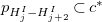 ${{{p}}_{{H}^I_j-{H}^I_{j+2}}} \subset {c}^*$
be the path connecting
 ${H}^I_j$
and
 ${H}^I_{j+2}$
.
Consider the polygon
 $R$
(dotted, in Figure 8) delimited by:
-
(i) the path
${{p}}_{s-e}$
; -
(ii) the perimeter of the convex hull
$\partial {\mathcal H}(I)$
from
${P}_e$
to
${H}^I_j$
; -
(iii) the path
${{p}}_{{H}^I_j-{H}^I_{j+2}}$
; -
(iv) the perimeter of the convex hull
$\partial {\mathcal H}(I)$
from
${H}^I_{j+2}$
to
${P}_s$
.


Clearly, the point
 ${H}^I_{j+1}$
lies in the interior of
 $R$
. In order to reach it without self-crossings,
 ${c}^*$
cannot pass through
 ${{p}}_{s-e}$
nor
 ${{p}}_{{H}^I_j-{H}^I_{j+2}}$
. On the other hand,
 ${c}^*$
cannot cross
 $\partial {\mathcal H}(I)$
between
 ${P}_e$
and
 ${H}^I_j$
(and from
 ${H}^I_{j+2}$
to
 ${P}_s$
) because, by definition of convex hull, there are no vertexes to be visited that are interior to polygon
 $Q$
and that do not belong to
 $\partial {\mathcal H}(I)$
. So,
 ${c}^*$
cannot reach
 ${H}^I_{j+1}$
.
From Theorem 4.7: the path
 ${{p}}_{s-e}$
is the current assignment. Polygon
 $Q$
is delimited by
 ${{p}}_{s-e}$
and the (dashed) segment
 $\overline {{P}_e {P}_s}$
.
 $I$
contains the points strictly inside
 $Q$
plus
 ${P}_s$
and
 ${P}_e$
;
 ${\mathcal H}(I)$
(grey in the picture) is its convex hull. Polygon
 $R$
is delimited by
 ${{p}}_{s-e}$
and the dotted segments.

Fig. 8. Long description
A diagram of a geometric constraint propagation process. The diagram features two polygons, one delimited by solid lines and a dashed segment, and another delimited by solid lines and dotted segments. The first polygon contains points strictly inside it, including points P_s and P_e, and is shown in grey. The convex hull of this polygon is also depicted. The second polygon is outlined by dotted segments. The diagram includes various labeled points and segments, such as H_j^I, H_{j+1}^I, H_{j+2}^I, Q, and R. Arrows indicate directions or flows between these points and segments. The overall structure shows the relationships and constraints between these geometric elements.
If we find an internal hull
 ${\mathcal H}(I)$
(see Figure 8), we can then apply the previous propagators (Algorithms2 and 3) also to
 $\partial {\mathcal H}(I)$
, with the obvious care that if
 ${{p}}_{s-e}$
reaches points in clockwise order, then
 $\partial {\mathcal H}(I)$
will be reached in counter-clockwise order (and vice versa). We maintain all partial paths during the search, and we compute a convex hull for each of these paths. In this way, we are orthogonal to heuristics (we can use any search heuristic without invalidating our propagation).
In the implementation, we applied the pruning on internal hulls only when the polygon
 $Q$
is convex. Checking the convexity amounts to check that each turn in the path is on the same side (a right turn, on a clockwise path), it makes it easier to find when a point is inside the polygon and also allows us to avoid checking that
 ${\mathcal H}(I)$
does not intersect
 ${{p}}_{s-e}$
.
The time complexity of our implementation of the extended convex hull is
 $O(n^2)$
to compute the points inside the polygon, then we use Andrew’s monotone chain (
 $O({n} \log {n})$
) (Andrew Reference Andrew1979) to find the hull. We currently recompute
 $\partial {\mathcal H}(I)$
from scratch after each decision.
5 Geometric reasoning for the Euclidean Generalized TSP
The propagation mechanisms developed in Section 4 are not limited to the Euclidean TSP, but can also be extended to other routing problems and variants of TSP that use the Euclidean distance as a metric. As an example, consider the Generalized Traveling Salesperson Problem (GTSP); in the GTSP, also known as set TSP, the set
 $V$
of nodes of the graph is partitioned into
 $C_1, \ldots , C_m$
subsets where each subset of nodes
 $C_i$
is called cluster and
 $C_j \cap C_k = \emptyset$
for all
 $j, k \in \lbrace 1, \ldots , m\rbrace$
. We use
 $C ({P}_i)$
to denote the cluster associated with point
 ${P}_i$
. The objective is to compute the minimum cost cycle that visits each cluster at least once. The GTSP has a wide number of applications (Noon and Bean Reference Noon and Bean1991; Laporte et al. Reference Laporte, Asef-Vaziri and Sriskandarajah1996) including sequencing of computer files, routing of welfare customers through governmental agencies, design of ring networks, flexible manufacturing scheduling, airport selection and routing for courier planes, and postal routing. The EGTSP, similarly to the ETSP, uses Euclidean distance as its metric and the coordinates of the points on the plane are known.
As in the ETSP, we employed the successor representation to model the EGTSP: the constraint model, see equation (3), involves n variables
 ${\text{ Next}}_i$
. Since in the EGTSP not all nodes are visited, we take the convention proposed in Francis and Stuckey (Reference Francis and Stuckey2014) that unvisited nodes have themselves as successors (i.e.
 ${\text{ Next}}_i = i$
); clearly this requires a modified version of the circuit constraint (Francis and Stuckey Reference Francis and Stuckey2014) that accepts subtours of length 1, see equation (3b). The model includes the alldifferent constraint, see equation (3a), to avoid two nodes from having the same successor, and a constraint imposing that at least one node is selected for each cluster, see equation (3c).
 \begin{align} {\tt alldifferent}({\text{ Next}}) & \end{align}
 \begin{align} {\tt set\_circuit}({\text{ Next}}) & \end{align}
 \begin{align} \sum _{i \in C_k} \vert {\text{ Next}}_i - i\vert \geq 1 & \;\;\; \forall k \in \lbrace 1, \ldots , m\rbrace \end{align}
Having introduced the constraint model, we now investigate how the geometric propagation developed for the ETSP can be adapted to the EGTSP.
In EGTSP we cannot directly apply the pruning introduced in Section 4.2 because the vertexes on the boundary of the convex hull may not be visited. Obviously in case such points are visited then they must be visited in the correct order, as already shown for the ETSP. In the following we will show how, under certain conditions, such pruning can also be extended to other “internal” points.
To simplify the following discussion, Definition5.1 introduces the concept of set of neighbors of a point on the boundary of the convex hull.
Definition 5.1. Given
 $H_i \in {\partial {\mathcal H}({\mathcal {P}})}$
a point
 ${P}_j \in {C (H_i)}$
is called a neighbor of
 ${H}_i$
if and only if the segment
 $\overline {{H}_i {P}_j}$
does not intersect
 ${\mathcal H}({\mathcal {P}} \setminus {C (H_i)})$
. The set
 ${\mathcal N} ({H}_i)$
is the set of all points
 ${P}_j \in {C (H_i)}$
that are neighbors of
 ${H}_i$
(by definition
 ${H}_i \in {{\mathcal N} ({H}_i)}$
).
In the example in Figure 9, points have a color representing the cluster they belong to. Among the points in the green cluster, only
 ${P}_k$
is not a neighbor of
 ${H}_i$
, because the segment
 $\overline {{H}_i {P}_k}$
intersects the convex hull
 ${\mathcal H}({\mathcal {P}} \setminus {C (H_i)})$
of the non-green points.
Now we can extend the reasoning of the convex hull to the GTSP.
From Definition5.1
 ${P}_k$
is not a neighbor of
 ${H}_i$
because the segment
 $\overline {{H}_i {P}_k}$
intersects the convex hull
 ${\mathcal H}({\mathcal {P}} \setminus {C (H_i)})$
.

Theorem 5.2. Let
 ${P}_g \equiv {H}_i$
be a point in
 $\partial {\mathcal H}({\mathcal {P}})$
, and let
 ${P}_b \equiv S({H}_i)$
be its successor in the sequence
 $\partial {\mathcal H}({\mathcal {P}})$
. Let
 $C_g$
and
 $C_b$
be the clusters containing
 ${P}_g$
and
 ${P}_b$
, respectively, with
 $C_g \neq C_b$
.
Let
 $ \Phi _{{P}_g} = {{\mathcal H}({{\mathcal N} ({P}_g)} \cup {{\mathcal N} ({P}_b)})}$
be the convex hull of the neighbors of
 ${P}_g$
and
 ${P}_b$
, and let
 $ \Phi _{{P}_g}^{'} = {{\mathcal H}( {\mathcal {P}} \setminus \left ( {C ({P}_g)} \cup {C ({P}_b)} \right ) )}$
be the convex hull of all points belonging to clusters other than
 $C_g$
and
 $C_b$
.
If
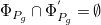 $\Phi _{{P}_g} \cap \Phi _{{P}_g}^{'} = \emptyset$
, then no point in
 ${\mathcal N} ({P}_b)$
can have a point in
 ${\mathcal N} ({P}_g)$
as its successor in any optimal EGTSP.
Proof. Let points
 ${P}_{g^{'}}$
and
 ${P}_{b^{'}}$
be neighbor of point
 ${P}_g$
and neighbor of point
 ${P}_b$
respectively, and let
 $c^{*}$
be an optimal EGTSP that includes both the point
 ${P}_{g^{'}}$
and the point
 ${P}_{b^{'}}$
. Firstly, we want to prove that both points
 ${P}_{g^{'}}$
and
 ${P}_{b^{'}}$
are in
 $\partial {\mathcal H}(c^{*})$
. By definition of neighbor of a point on the boundary of the convex hull, no point in the segment
 $\overline {{P}_g {P}_{g'}}$
is in
 ${\mathcal H}({\mathcal {P}} \setminus {C ({P}_g)})$
, so every point
 ${P}_j$
of the segment is on the border
 $\partial {\mathcal H}(\left ({\mathcal {P}} \setminus {C ({P}_g)}\right ) \cup \lbrace {P}_j \rbrace )$
. In an optimal EGTSP there is only one point for each cluster so if we have selected
 ${P}_{g^{'}}$
there cannot be any other point belonging to cluster
 $C_g$
, it follows that
 $c^{*} \subset {{\mathcal H}(\left ({\mathcal {P}} \setminus {C ({P}_g)}\right ) \cup \lbrace {P}_{g^{'}} \rbrace )}$
; since
 ${P}_{g^{'}} \in {\partial {\mathcal H}(\left ( {\mathcal {P}} \setminus {C ({P}_g)}\right ) \cup \lbrace {P}_{g^{'}} \rbrace )}$
, also
 ${P}_{g^{'}} \in {\partial {\mathcal H}(c^{*})}$
. A similar argument holds for the point
 ${P}_{b^{'}}$
, so we proved that they are both points in
 $\partial {\mathcal H}(c^{*})$
.
Suppose now, by contradiction, that
 ${P}_{b^{'}}$
has
 ${P}_{g^{'}}$
as its successor in
 $c^{*}$
(see Figure 10a). Since
 ${P}_{g'}$
is in the border
 $\partial {\mathcal H}(c^{*})$
, the angle formed by the segment
 $\overline {{P}_{b'} {P}_{g'}}$
and the segment from
 ${P}_{g'}$
to its successor must correspond to a right turn (it must be between
 $-\pi$
and
 $0$
). It follows that the successor of
 ${P}_{g'}$
in
 $c^*$
, denoted by
 $P_k$
, must be to the right of the straight line
 $\overleftrightarrow {{P}_{b'} {P}_{g'}}$
for
 $c^{*}$
to be optimal.
According to the position of the point
 ${P}_k$
, it is necessary to distinguish 3 different cases.
In the first case the point
 ${P}_k$
lies in the interior of polygon
 ${P}_b{P}_b^{'}{P}_g{P}_g^{'}$
and therefore
 ${P}_k \in \Phi _{{P}_g}$
but simultaneously
 ${P}_k \in \Phi _{{P}_g}^{'}$
because
 ${C ({P}_k)} \neq {C ({P}_g)}$
and
 ${C ({P}_k)} \neq {C ({P}_b)}$
contradicting the condition
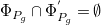 $\Phi _{{P}_g} \cap \Phi _{{P}_g}^{'} = \emptyset$
(see Figure 10b).
In the second case both segments
 $\overline {{P}_{k} {P}_{g'}}$
and
 $\overline {{P}_{k} {P}_{b'}}$
intersect the segment
 $\overline {{P}_{g} {P}_{b}}$
so it is not true that
 ${P}_b$
is the successor of
 ${P}_g$
in
 $\partial {\mathcal H}({\mathcal {P}})$
(see Figure 10c).
If the first two cases do not occur then either
 $\overline {{P}_{k} {P}_{b'}}$
intersects
 $\overline {{P}_{g} {P}_{g'}}$
or
 $\overline {{P}_{k} {P}_{g'}}$
intersects
 $\overline {{P}_{b} {P}_{b'}}$
. In the case where
 $\overline {{P}_{k} {P}_{b'}}$
intersects
 $\overline {{P}_{g} {P}_{g'}}$
it means that
 ${\mathcal H}({\mathcal {P}} \setminus {C ({P}_g)})$
intersects
 $\overline {{P}_{g} {P}_{g'}}$
so
 ${P}_{g'}$
by definition cannot be a neighbor of
 ${P}_g$
(see Figure 10d). For the same reason
 ${P}_{b'}$
is not neighbor of
 ${P}_b$
if
 $\overline {{P}_{k} {P}_{g'}}$
intersects
 $\overline {{P}_{b} {P}_{b'}}$
.
From Theorem 5.2
 ${P}_{b^{'}}$
cannot have
 ${P}_{g^{'}}$
as successor in any optimal EGTSP if
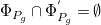 $\Phi _{{P}_g} \cap \Phi _{{P}_g}^{'} = \emptyset$
.

Fig. 10. Long description
Panel A: A diagram showing a configuration with a highlighted region labeled Phi’_Pg and a path from Pb to Pg’. Various colored shapes are scattered within the diagram. Panel B: A diagram with a highlighted region labeled Phi_g and paths from Pb to Pg and Pk. Different colored shapes are distributed within the diagram. Panel C: A diagram with a highlighted region labeled Phi_g and paths from Pb to Pg’, Pk, and Pg. Various colored shapes are present within the diagram. Panel D: A diagram with a highlighted region labeled Phi_g and paths from Pb to Pg’, Pk, and Pg. Different colored shapes are distributed within the diagram.
The implementation of a propagator exploiting Theorem 5.2 is given in Algorithm 4.
In the proof of the Theorem 5.2 we also proved that neighbors of a point in
 $\partial {\mathcal H}({\mathcal {P}})$
, if selected, will be on the boundary of the convex hull of the optimal solution so it is possible to impose the clockwise constraint (see Section 4.2) on them as well. In the experimental evaluation, we applied only the reasoning on the angle formed by the incoming and the outgoing arcs in hull vertexes, using the easiest implementation, which consists of waiting until variables become instantiated with a value.
hull_set_propagator

6 Experimental evaluation
To assess the effectiveness of the proposed algorithms, we devised experiments for both Euclidean TSPs and Euclidean Generalized TSPs. All algorithms are implemented in the ECL
 $^i$
PS
 $^e$
CLP language (Schimpf and Shen Reference Schimpf and Shen2012). All tests were run on ECL
 $^i$
PS
 $^e$
v. 7.0, build #48, with a time limit of 1800s on
 $\textrm {Intel}^{\circledR }$
 $\textrm {Xeon}^{\circledR }$
E5-2630 v3 CPUs running at 2.4 GHz, using only one core and with 2 GB of reserved memory. The ECL
 $^i$
PS
 $^e$
Constraint Programming System is distributed as open-source software.Footnote
1
The implementation uses the suspension and event-based wake-up facilities provided by ECL
 $^i$
PS
 $^e$
. These facilities are used to react to domain modifications or variable instantiation and to reschedule the propagators only when relevant changes occur. However, the filtering rules are not specific to ECL
 $^i$
PS
 $^e$
. They can be ported to other CLP or CP systems that support user-defined propagators, inspection and modification of finite domains, and event-based activation on domain changes.
6.1 Euclidean TSP
Euclidean TSP constraint model is based on the successor representation described in the preliminaries (with the
 $\tt circuit$
constraint and
 $\tt alldifferent$
(Puget Reference Puget1998) for improved pruning) with both
 $\text{ Next}$
and
 $\text{ Prev}$
variables, that are linked through the inverseconstraint. In this section we compare different constraint models extending the one presented in the preliminaries by adding additional constraints.
In the following we denote by
 $GEO$
the constraint model that adds the
 $\tt nocrossing$
constraint, the removal of aligned points according to Proposition4.3, and the clockwiseconstraint that implements the propagation described in Section 4.2.
In order to show that the pruning we provide is not subsumed by that of state-of-the-art techniques, we implemented in ECL
 $^i$
PS
 $^e$
, in the successor representation, also the Held and Karp bound with pruning based on Reduced and Marginal Costs, as proposed by Benchimol et al. (Reference Benchimol, van Hoeve, Régin, Rousseau and Rueher2012) (shown with HK-RMC in the following). The purpose of this comparison is to isolate the incremental effect of the proposed geometric propagation within a common CLP implementation.
As search strategies, we use the MAX-REGRET (Caseau and Laburthe Reference Caseau and Laburthe1997) and the state-of-the-art LC_FIRST MAX_COST (Fages et al. Reference Fages, Lorca and Rousseau2016), based on Last Conflict (Lecoutre et al. Reference Lecoutre, Saïs, Tabary and Vidal2009). As (Benchimol et al. Reference Benchimol, van Hoeve, Régin, Rousseau and Rueher2012), we also experimented injecting the upper bound given by the Lin-Kernighan-Helsgaun (LKH) (v. 2.0.7) algorithm.
We experimented both with structured and with random (unstructured) instances.
6.1.1 Structured instances
Structured instances model the position of real locations or sets of points from real-world problems. We consider instances taken from the TSPLIB (Reinelt Reference Reinelt1991), the Concorde websiteFootnote 2 and the CITIES datasetFootnote 3 up to 100 nodes. These sources provide various types of instances, amongst which Euclidean ones, represented as sets of points in the plane, and geographical ones, represented as sets of points (with latitude and longitude) on the surface of the Earth. In order to have a more complete set of instances, we decided to consider also geographical instances in which the cities to be visited lie on a limited part of the geoid, so that the geographical distance can be approximated with the Euclidean distance.
Table 1 reports the results for the 19 structured instances for which at least one configuration reached the optimal solution within the 1800-second time limit. Six of the 25 tested instances were omitted because all compared configurations reached the time limit. Each instance listed in the table is represented by its name, followed by the solving time (in seconds) and the number of search nodes required to find the optimal solution and prove its optimality. Aside from simple instances, the constraint models that contain geometric filtering are the ones that optimally solve the instances in the shortest time. These results show the positive interaction between the geometric filtering and that carried out by HK-RMC alone. By analyzing the instances that were not solved to optimality, we found that our additional pruning is more effective during the proof of optimality, rather than on finding good initial solutions.
Comparing filtering algorithms on structured instances with time limit 1800s. For each instance we report total solving time and number of explored nodes to reach the optimal solution and prove its optimality

Table 1. Long description
A table comparing filtering algorithms on structured instances with solving time and number of explored nodes. The table has 19 rows and 8 columns. Column headers are LC_FIRST_MAX_COST, MAX-REGRET, HK-RMC CPU time, HK-RMC nodes, GEO+HK-RMC CPU time, GEO+HK-RMC nodes, HK-RMC CPU time, and HK-RMC nodes. Row labels are instance names. Row 1: uk12, 0.04, 12, 0.05, 12, 0.04, 1, 0.04, 1. Row 2: burma14, 0.06, 14, 0.07, 14, 0.05, 1, 0.07, 1. Row 3: ulysses16, 0.07, 16, 0.09, 16, 0.07, 1, 0.08, 1. Row 4: ulysses22, 0.12, 22, 0.15, 22, 0.12, 1, 0.16, 1. Row 5: wg22, 0.14, 22, 0.18, 22, 0.13, 1, 0.17, 1. Row 6: bavg29, 0.45, 30, 0.44, 35, 0.41, 3, 0.43, 2. Row 7: wi29, 0.23, 29, 0.32, 29, 0.23, 1, 0.32, 1. Row 8: dj38, 0.42, 38, 0.65, 38, 0.42, 1, 0.65, 1. Row 9: dantzig42, 2.16, 48, 1.60, 43, 4.83, 28, 2.11, 3. Row 10: att48, 3.21, 66, 2.38, 55, 8.02, 36, 3.10, 10. Row 11: uscup50, 0.64, 50, 1.22, 50, 0.64, 1, 1.22, 1. Row 12: ei51, T/O, -, 523.92, 1384, 313.53, 916, 84.43, 195. Row 13: berlin52, 0.86, 52, 1.67, 52, 0.84, 1, 1.52, 1. Row 14: kn57, 8.53, 180, 5.67, 120, 8.24, 38, 5.14, 18. Row 15: wg59, 1.13, 59, 1.92, 59, 1.35, 1, 1.8, 1. Row 16: st70, 1411.63, 3934, 327.79, 985, T/O, -, T/O, -. Row 17: eil76, 72.56, 227, 33.20, 156, 160.09, 230, 31.8, 26. Row 18: rat99, T/O, -, T/O, -, T/O, -, 436.97, 574. Row 19: rd100, 25.81, 117, 21.79, 107, 52.99, 80, 21.94, 22.
Note: Bold values indicate the best result in each row.
6.1.2 Random instances
Random or unstructured instances consist of points with random coordinates on the plane. In the literature (Fischetti and Toth Reference Fischetti and Toth1992; Johnson and McGeoch Reference Johnson and McGeoch2007), typically two types of instances are considered: uniform and clustered. Instances of the uniform class are obtained by placing points in the plane according to a uniform distribution, while clustered instances consist of clusters of points, whose centers are uniformly distributed in the plane. Random instances have been generated through the R-package netgen (Bossek Reference Bossek2015) and its functions: generateRandomNetwork, generateClusteredNetwork. The function generateRandomNetworkgenerates a random graph by placing points uniformly distributed in a
 $10^6 \times 10^6$
square. The function generateClusteredNetworkinitially generates cluster centers by Latin Hypercube Sampling (LHS) to ensure that the clusters are placed separately from each other. Then it distributes points to the clusters according to a normal distribution having as mean vector the centers of the clusters and as variance the distance to the center of the nearest neighbor cluster.
Comparing solving time 11a, 11b and search nodes 11c, 11d of HK-RMC and GEO+HK-RMC models on randomly-generated Euclidean TSP instances belonging to the uniform class when LC_FIRST MAX_COST search strategy is used. The solving time limit was set to 1800 s. Each data point in these figures corresponds to an instance. We removed instances where both models ran into timeout.

Fig. 11. Long description
Four graphs compare the performance of HK-RMC and GEO+HK-RMC models on randomly-generated Euclidean TSP instances. Panel A is a scatter plot showing CPU time with GEO+HK-RMC on the vertical axis and HK-RMC on the horizontal axis. The number of nodes is indicated by different symbols and colors. Panel B is a box plot comparing CPU time for different ranges of nodes, with HK-RMC in gray and GEO+HK-RMC in yellow. Panel C is a scatter plot showing search nodes with GEO+HK-RMC on the vertical axis and HK-RMC on the horizontal axis, with the number of nodes indicated by different symbols and colors. Panel D is a box plot comparing search nodes for different ranges of nodes, with HK-RMC in gray and GEO+HK-RMC in yellow. The solving time limit was set to 1800 seconds, and instances where both models ran into timeout were removed.
Comparing solving time 12a, 12b and search nodes 12c, 12d of HK-RMC and GEO+HK-RMC models on randomly-generated Euclidean TSP instances belonging to the uniform class when MAX-REGRET search strategy is used. The solving time limit was set to 1800 s. Each data point in these figures corresponds to an instance. We removed instances where both models ran into timeout.

Fig. 12. Long description
Four graphs compare the solving time and search nodes of HK-RMC and GEO+HK-RMC models on randomly-generated Euclidean TSP instances. Panel A: A scatter plot compares CPU time for HK-RMC and GEO+HK-RMC models. The x-axis represents CPU time for HK-RMC in seconds, and the y-axis represents CPU time for GEO+HK-RMC in seconds. Different symbols and colors represent different ranges of the number of nodes. Panel B: A box plot compares CPU time for HK-RMC and GEO+HK-RMC models across different ranges of the number of nodes. The x-axis represents the number of nodes, and the y-axis represents CPU time in seconds. Panel C: A scatter plot compares the number of search nodes for HK-RMC and GEO+HK-RMC models. The x-axis represents the number of search nodes for HK-RMC, and the y-axis represents the number of search nodes for GEO+HK-RMC. Different symbols and colors represent different ranges of the number of nodes. Panel D: A box plot compares the number of search nodes for HK-RMC and GEO+HK-RMC models across different ranges of the number of nodes. The x-axis represents the number of nodes, and the y-axis represents the number of search nodes.
We randomly generated instances from 20 to 100 nodes in steps of 2, in both classes. For each size in the uniform class we generated 32 instances, for a total of 1312 instances. For the clustered class we tested
 $n.cluster = 3, 5, 8, 11$
as number of clusters; for each size and number of clusters we generated 16 instances, for a total of 2624 instances. For the uniform class, 276 of the 1312 generated instances (21.0%) were excluded from the plots and aggregate statistics because all compared configurations reached the 1800-second time limit. For the clustered class, this occurred for 960 of the 2624 generated instances (36.6%).
In Figure 11, we present log–log scatter plots and boxplots comparing the GEO+HK-RMC model, which includes our filtering algorithm, to the HK-RMC model when solving uniform instances with the LC_FIRST MAX_COST search strategy. Figure 11a and 11b compare the solving time, while Figure 11c and 11d compare the search nodes. Figure 11a shows that the solving time is significantly reduced when the GEO+HK-RMC model is used compared to HK-RMC. The reduction in solving time is evident across all node ranges, with the most substantial improvements observed for larger instances. On average, there is a 70% reduction in solving time when our filtering is used. Figure 11b provides a boxplot representation of the solving time across different instances size; note that, even on a logarithmic scale, the gap between the median solving times increases with the problem size, reaching an order of magnitude for instances with 80 or more nodes, despite the saturating effect of the timeout encountered by the competitor method for larger instance sizes. Figure 11c and 11d show the number of search nodes required to reach a solution. Similar to the solving time, the GEO+HK-RMC model consistently requires fewer search nodes than the HK-RMC model, with an average reduction of 59%. Notably, this reduction holds even though, in timeout cases, the node count includes only the nodes explored up to the timeout threshold, potentially underestimating the effort required by the HK-RMC model and thus disadvantaging the GEO+HK-RMC model.
In Figure 12, we present similar log–log scatter plots and boxplots comparing the GEO+HK-RMC and HK-RMC constraint models when using the MAX-REGRET search strategy. As with LC_FIRST MAX_COST, the GEO+HK-RMC model achieves substantial improvements in both solving time and number of search nodes. Specifically, it reduces solving time by an average of 70% and the number of search nodes by 71%, with nearly all instances lying below the diagonal in the scatter plots. Notably, several small instances are solved by the GEO+HK-RMC model using just one search node. Similar issues with timeouts apply here as well. When an instance times out, we only count the nodes explored up to the time limit. This likely underestimates how many nodes the HK-RMC model would actually need, making the comparison unfairly harder for our model.
Table 2 presents the number of instances that reached the timeout limit of 1800 s during the experiments for various configurations of nodes and constraint models. The results indicate that for small instances (20 to 38 nodes), both algorithms performed similarly well with almost no instances reaching the timeout. As the dimension increased, the GEO+HK-RMC algorithm consistently outperformed HK-RMC, particularly with the LC_FIRST MAX_COST search strategy. For example, in the 90-100 node range, GEO+HK-RMC with LC_FIRST MAX_COST had 119 timeouts compared to 144 of HK-RMC.
Number of uniform instances that were not solved within the timeout during experiments, grouped by size (shown as node ranges). The experiments compared the HK-RMC and GEO+HK-RMC constraint models, with the MAX-REGRET and LC_FIRST MAX_COST search strategies

Table 2. Long description
The table presents the number of uniform instances that were not solved within the timeout during experiments, grouped by node ranges. It compares the HK-RMC and GEO+HK-RMC constraint models with the MAX-REGRET and LC_FIRST MAX_COST search strategies. The table has 5 columns: the first column lists the node ranges (20-28, 30-38, 40-48, 50-58, 60-68, 70-78, 80-88, 90-100), and the remaining four columns show the number of unsolved instances for each combination of constraint model and search strategy. For node ranges 20-28 and 30-38, all values are 0 or 1, indicating similar performance. As the node range increases, the GEO+HK-RMC model generally shows fewer unsolved instances compared to HK-RMC, especially with the LC_FIRST MAX_COST strategy. For example, in the 90-100 node range, GEO+HK-RMC with LC_FIRST MAX_COST has 119 unsolved instances, while HK-RMC has 144.
Note: Bold values indicate the best result in each row.
Experiments on clustered instances, as shown in Figure 13, confirm that the use of geometric filtering significantly reduces the average solving time by 70% when compared to the HK-RMC model alone.
Figure 13a presents a log–log scatter plot comparing the solving time of the GEO+HK-RMC model with the HK-RMC model across different node ranges and cluster counts when LC_FIRST MAX_COST search strategy is used. Each point represents an instance, and the results show a clear reduction in solving time for the GEO+HK-RMC model. Figure 13b shows a similar scatter plot but focuses on the number of search nodes. The GEO+HK-RMC model consistently requires fewer search nodes to reach a solution, indicating more efficient search performance.
Figure 13c and Figure 13d replicate the analysis using the MAX-REGRET search strategy. Figure 13c shows the solving time comparison, while Figure 13d presents the number of search nodes. The patterns observed are similar to those with the LC_FIRST MAX_COST strategy, further validating the robustness of the GEO+HK-RMC model.
Specifically, the GEO+HK-RMC model provided substantial reductions in the number of explored nodes: a 43% reduction with the LC_FIRST MAX_COST strategy and a 75% reduction with the MAX-REGRET search strategy. From Figure 13, it can also be observed that the number of clusters does not significantly affect the solving performance of the two constraint models. This suggests that the improvements provided by the geometric filtering are robust across varying cluster configurations.
Comparing solving time and search nodes of HK-RMC and GEO+HK-RMC models on randomly-generated Euclidean TSP instances belonging to the clustered class varying the number of clusters (shown by the different colors). Figure 13a and 13b show the results obtained using the LC_FIRST MAX_COST search strategy while Figure 13c and 13d show the results obtained using the MAX-REGRET search strategy. The solving time limit was set to 1800 s. We removed instances where both models ran into timeout.

Fig. 13. Long description
Four scatter plots compare solving time and search nodes of two models on Euclidean TSP instances with varying clusters. Panel A: A scatter plot shows CPU time in seconds on a logarithmic scale for both axes. The x-axis represents HK-RMC, and the y-axis represents GEO+HK-RMC. Different symbols and colors indicate the number of nodes and clusters. Panel B: A scatter plot shows search nodes on a logarithmic scale for both axes. The x-axis represents HK-RMC, and the y-axis represents GEO+HK-RMC. Different symbols and colors indicate the number of nodes and clusters. Panel C: A scatter plot shows CPU time in seconds on a logarithmic scale for both axes using the MAX-REGRET search strategy. The x-axis represents HK-RMC, and the y-axis represents GEO+HK-RMC. Different symbols and colors indicate the number of nodes and clusters. Panel D: A scatter plot shows search nodes on a logarithmic scale for both axes using the MAX-REGRET search strategy. The x-axis represents HK-RMC, and the y-axis represents GEO+HK-RMC. Different symbols and colors indicate the number of nodes and clusters.
Number of clustered instances that reached the timeout limit of 1800 s during the experiments, grouped by different numbers of clusters and sizes (shown as node ranges). The experiments compared the HK-RMC and GEO+HK-RMC algorithms, with the MAX-REGRET and LC_FIRST MAX_COST search strategies

Table 3. Long description
The table presents the number of clustered instances that reached the timeout limit of 1800 seconds during experiments, grouped by different numbers of clusters and node ranges. The experiments compared the HK-RMC and GEO+HK-RMC algorithms using the MAX-REGRET and LC_FIRST MAX_COST search strategies. The table has 4 rows and 8 columns. Column headers are: # clusters, # nodes, MAX-REGRET HK-RMC, MAX-REGRET GEO+HK-RMC, LC_FIRST MAX_COST HK-RMC, LC_FIRST MAX_COST GEO+HK-RMC. Row labels are: 3, 5, 8, 11. Each row contains values for different node ranges (20-28, 30-38, 40-48, 50-58, 60-68, 70-78, 80-88, 90-100). Notable trends include varying numbers of instances reaching the timeout limit across different cluster sizes and node ranges, with some combinations showing higher timeout occurrences than others.
Note: Bold values indicate the best result in each row.
Table 3 presents the number of clustered instances that reached the timeout limit of 1800 s during the experiments, categorized by different configurations of clusters, dimensions, and constraint model. The trend concerning the instance size mirrors that observed in the uniform instances. For smaller instances (up to 68 nodes), the MAX-REGRET strategy generally performs better. However, for larger instances, the LC_FIRST MAX_COST strategy shows superior performance. As for the constraint models, the GEO+HK-RMC model consistently outperforms the HK-RMC model across different configurations. When analyzing the number of clusters, a clear pattern emerges: instances with a higher number of clusters are generally easier to solve, as reflected by the reduced number of timeouts. This suggests that increasing the number of clusters simplifies the problem structure, making instances more tractable within the given time limit.
6.2 Euclidean generalized TSP
The instances for the GTSP in the literature (Laporte and Nobert Reference Laporte and Nobert1983; Laporte et al. Reference Laporte, Mercure and Nobert1987; Fischetti et al. Reference Fischetti, González and Toth1997) are normally created from existing structured (see Section 6.1.1) or random (see Section 6.1.2) instances. Starting from random TSP instances, we experimented with three approaches to partition points into clusters.
Once a number of clusters
 $c$
is fixed, the uniform approach (inspired by Laporte and Nobert (Reference Laporte and Nobert1983); Laporte et al. (Reference Laporte, Mercure and Nobert1987)) distributes with uniform probability the points among the clusters.
The clustering approach was proposed by Fischetti et al. (Reference Fischetti, González and Toth1997). For an instance with
 $n$
points, the number of clusters is set to
 $c = \lceil n/5\rceil$
. Then
 $c$
points, that will represent the centers of the clusters, are selected to be as far away as possible from each other. The remaining points are then associated with the nearest center.
The grid approach was also proposed by Fischetti et al. (Reference Fischetti, González and Toth1997). Consider the minimum rectangle with sides parallel to the coordinate axes enclosing all points in the instance. The rectangle is subdivided in an
 $L \times L$
grid, and each grid cell containing at least one point is a cluster. The value
 $L$
is determined so that each cluster contains an average number
 $\mu$
of nodes, let
 $\mbox{CLUSTER}(H)$
be the number of clusters corresponding to an
 $H \times H$
grid,
 $L$
is defined as the smallest integer such that
 $\mbox{CLUSTER}(L) \geq n/\mu$
.
As in the case of the ETSP, we compare two constraint models based on the successor representation. The first model, denoted by ECLP, includes the basic model for the EGTSP described in equation (3). The second model, called GEO, adds the geometric pruning based on the convex hull introduced in Section 5. For all experiments we used the max-regret (Caseau and Laburthe Reference Caseau and Laburthe1997) search strategy.
We randomly generated instances from 20 to 50 nodes, using the three previously introduced approaches. For instances generated using the grid approach we set the parameter
 $\mu = 5$
. For each size and each approach we generated 16 instances, for a total of 1488 instances. Of these 1488 instances, 424 (28.5%) were excluded from the plots and aggregate statistics because all compared configurations reached the 1800-second time limit.
Figure 14 compares the experimental results of the two models using a cactus plot, showing the number of solved instances as a function of the CPU time. The GEO model consistently outperforms the reference ECLP model by solving more instances within the same time limit.
In addition to solving a higher number of instances, the GEO model also achieves a consistent reduction in both computation time and number of explored nodes across all instance types. If we consider instances generated with the clustering approach the average solving time with the GEO model is reduced by 76% and the average number of nodes explored is reduced by 77%. For grid type instances the results are similar as the reduction of the average solving time results 67% together with a reduction of the average number of explored nodes by 66%.
For uniform type instances the average solving time is reduced by 19% and the average number of search nodes by 17%. These slightly lower results can be attributed to the distribution of points that makes it difficult to have sets of neighbors of significant size in the instances. Since the filtering algorithm relies on sets of neighbors their absence weakens the pruning. However, the results overall show that our approach is definitely useful in improving solving performance.
Comparing number of solved instances by ECLP and GEO models on Euclidean GTSP instances generated using different approaches to partition points into clusters. The solving time limit was set to 1800 s. We removed instances where both models ran into timeout.

Fig. 14. Long description
A line graph comparing the number of solved instances by ECLP and GEO models on Euclidean GTSP instances using different partitioning approaches. The horizontal axis represents the number of solved instances, ranging from 200 to 400. The vertical axis represents CPU time in seconds, ranging from 0 to 2000. The graph includes six data series: ECLP uniform, GEO uniform, ECLP grid, GEO grid, ECLP clustering, and GEO clustering. Each series is represented by a different line style and color. The ECLP uniform and GEO uniform lines show a steady increase in CPU time as the number of solved instances increases. The ECLP grid and GEO grid lines also show a similar trend but with slightly higher CPU times. The ECLP clustering and GEO clustering lines exhibit a more rapid increase in CPU time, indicating that these methods require more computational resources as the number of solved instances grows.
Overall, the main practical benefit of the proposed geometric propagators is a reduction of the search space, rather than merely a lower constant cost per search node. On the random ETSP instances, the number of explored nodes is reduced by 43–75%, depending on the instance class and search strategy. This reduction is accompanied by lower solving times and fewer timeouts, especially for the larger tested instances. A similar behavior is observed for the EGTSP, where the geometric model explores fewer nodes and solves more instances within the time limit. The complexity improvement discussed for the nocrossing propagator concerns its implementation relative to a naive propagator; we do not claim an improvement in the asymptotic complexity of solving the TSP.
7 Conclusions
In this article, we showed the effectiveness of the use of geometric information in routing problems. While the most common approach in Constraint Programming and related research areas is to address the Euclidean Traveling Salesperson Problem with the same constraint model as the general TSP, we showed that the use of the additional information naturally available in many TSP instances can provide further pruning and speed up the search. In fact, in the ETSP the coordinates of the points in the plane are known, and while the common approach is to use such knowledge only to compute the distance matrix and disregarding it in the constraint model, we employed it to strengthen the constraint model with additional redundant constraints that effectively reduce the search space.
This article is a revised and extended version of a conference publication Bertagnon and Gavanelli (Reference Bertagnon and Gavanelli2020), which, to the best of our knowledge, was the first work to exploit the classical no-crossing and convex-hull ordering properties through dedicated propagation mechanisms in a successor-based CP/CLP model for the Euclidean TSP.
However, while Bertagnon and Gavanelli (Reference Bertagnon and Gavanelli2020) showed the effectiveness of the idea only in the TSP problem (without any variation that can occur in real life problems), in this article we showed how the use of geometric information can be exploited also in the EGTSP, achieving a speedup of up to 4.2
 $\times$
in solving time and a reduction by a similar factor in the number of explored nodes. We provided a comprehensive and detailed exposition of the techniques we developed; a thorough and systematic experimentation campaign showed the effectiveness of the proposed algorithms.
As no CP models for the EGTSP were found in the literature, we proposed a first constraint model; again, the addition of geometric reasoning let us reduce the average solving time to
 $1/3$
on clustered instances and to
 $4/5$
on uniform instances.
Our results are not yet comparable with those obtained by state-of-the-art TSP solvers, such as Concorde, but on the other hand Concorde cannot solve GTSP instances. Also note that the implementation of the proposed algorithms is based on a declarative approach and on the open-source Constraint Logic Programming solver ECL
 $^i$
PS
 $^e$
. Indeed, the aim of this research was to show that exploiting geometric information can result in stronger pruning rather than proposing a very fast and efficient algorithm which would probably have required an implementation in an imperative language. We believe that the same techniques can nevertheless also be exploited in solvers implemented in imperative languages.
One limitation of the current work is that it is not universally applicable to all TSP variants, such as the TSP with Time Windows, since its optimal solutions may contain crossings; but crossings avoidance could also be interesting per se in some applications. As future work, we plan to investigate extensions of the proposed techniques to other routing models in which the geometric structure and the feasible connections preserve the assumptions required by the proposed pruning.
Competing interests
The authors declare none.


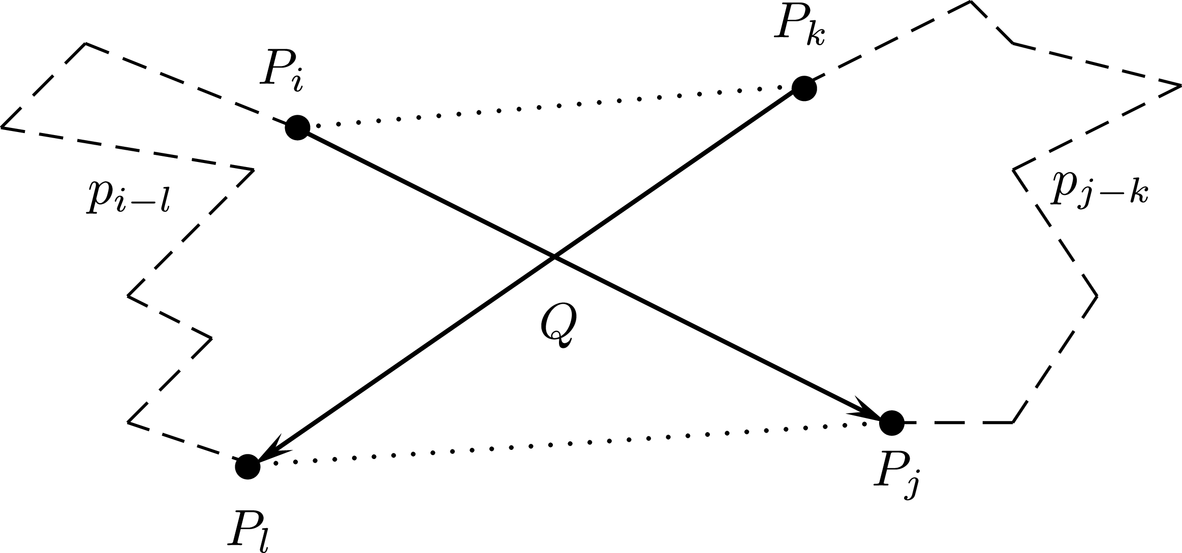
 PiPj¯
 PkPl¯
 PiPk¯
 PjPl¯
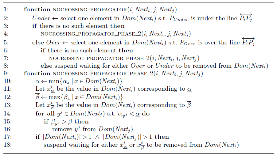
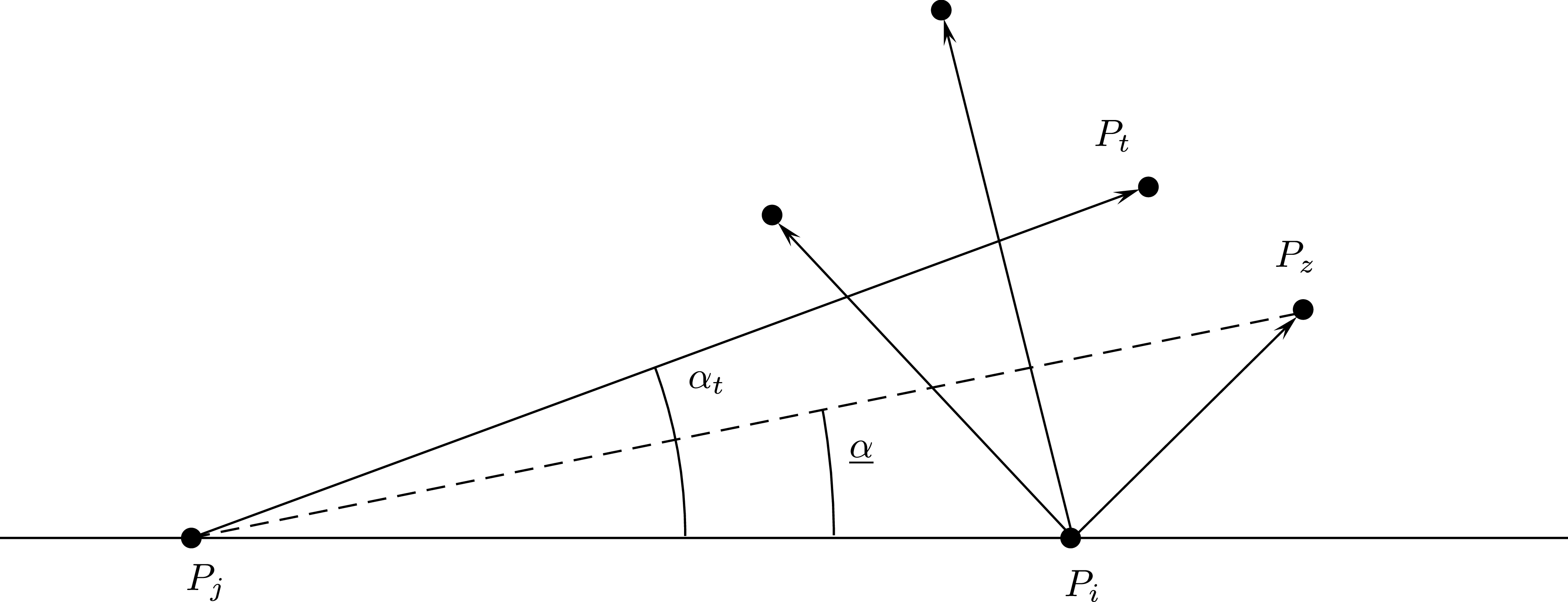
 Px
 Py
 y∈Dom( Nextx)
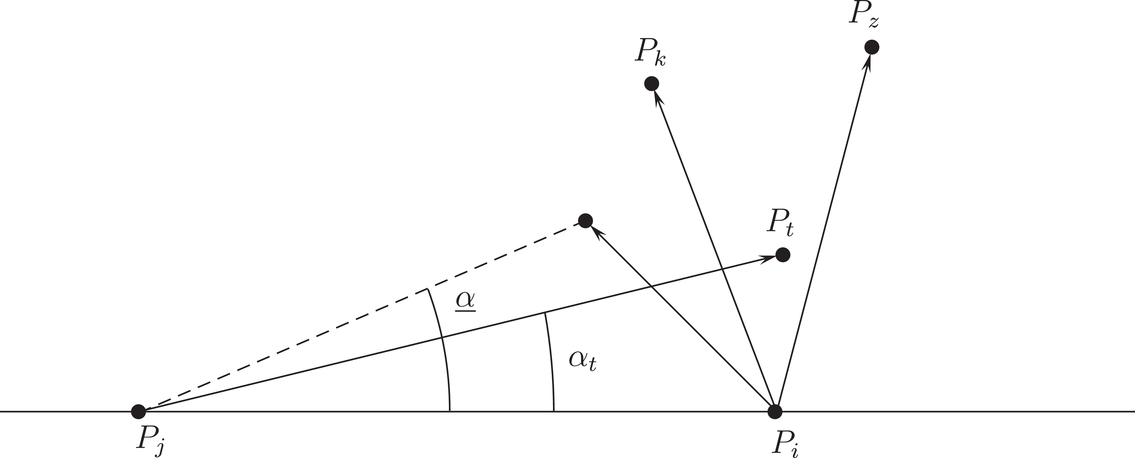
 αt<α_
 PjPt¯
 Pi
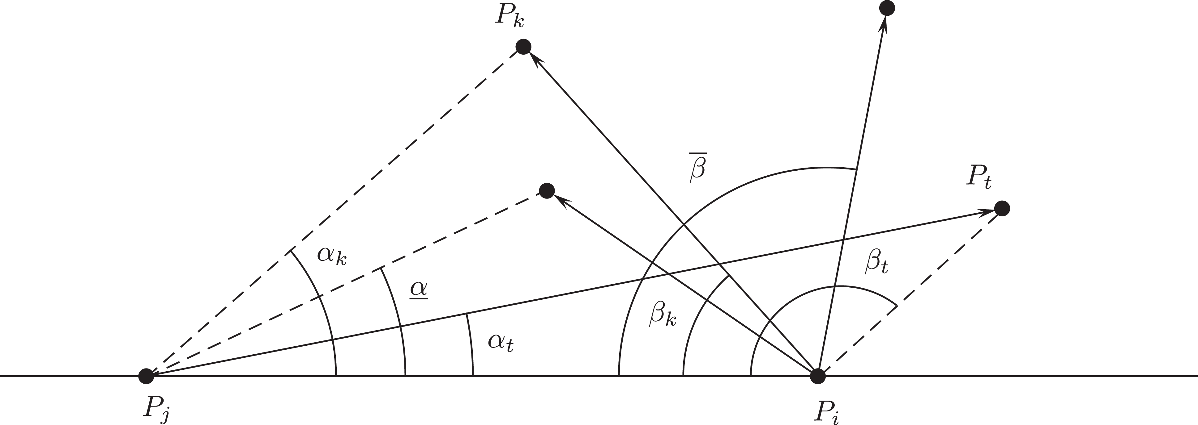
 Px
 Py
 y∈Dom( Nextx)
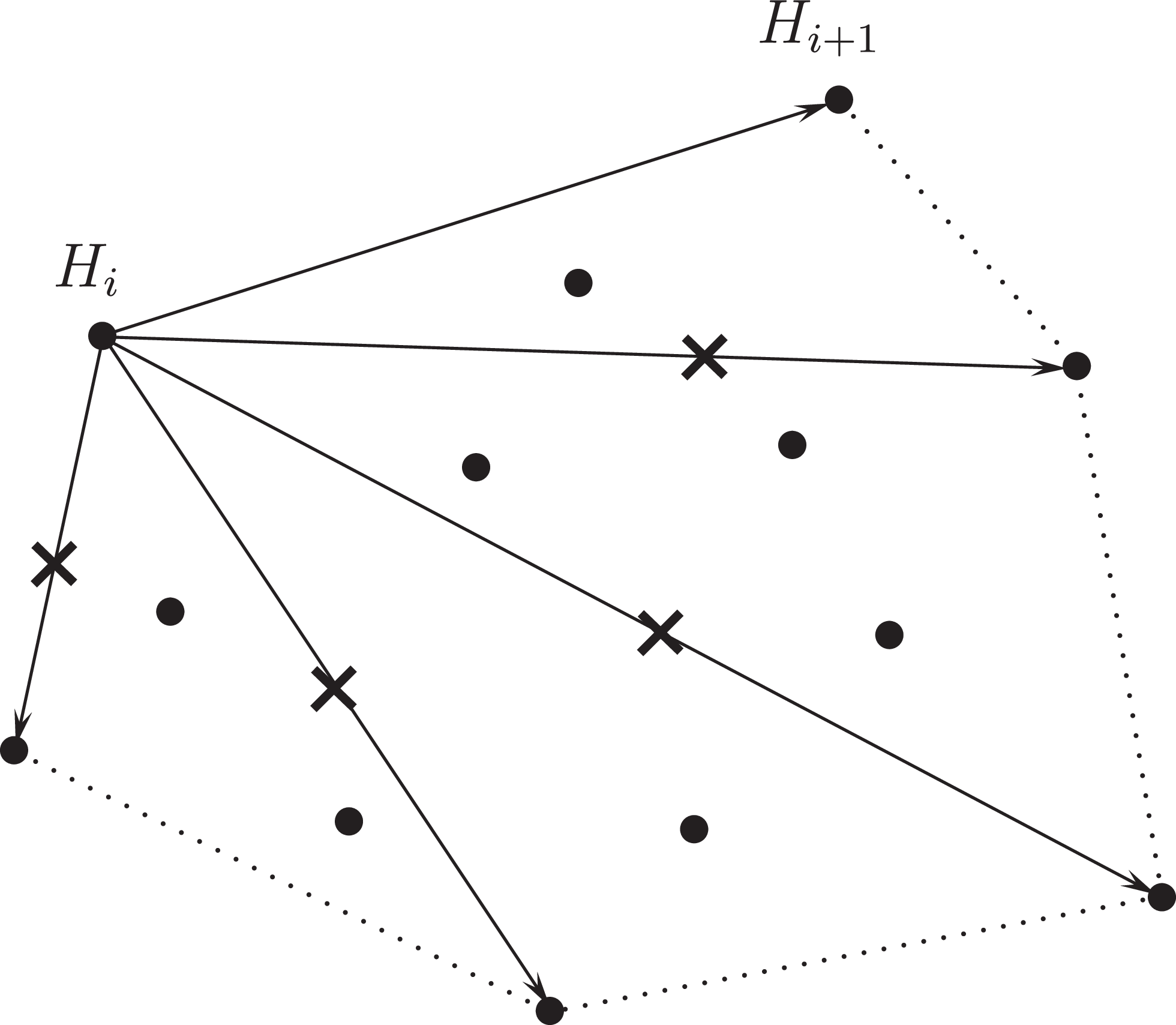
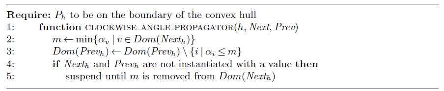
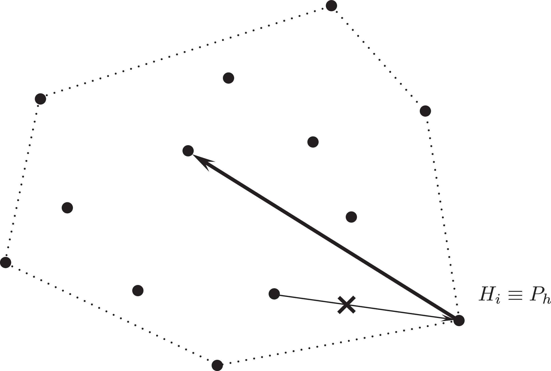
 −π
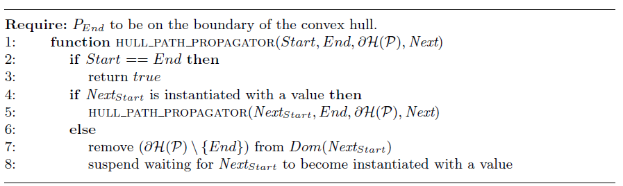
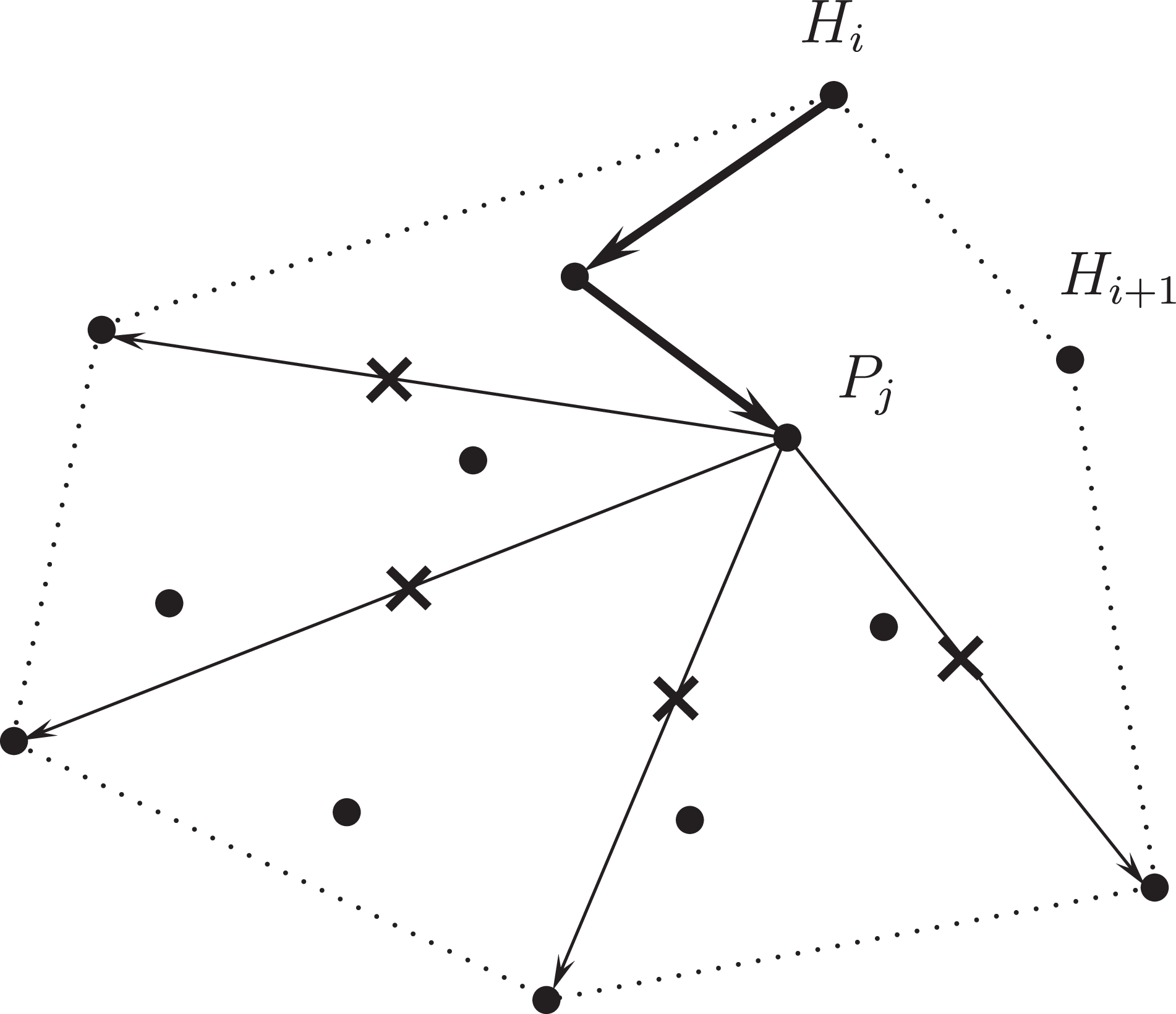
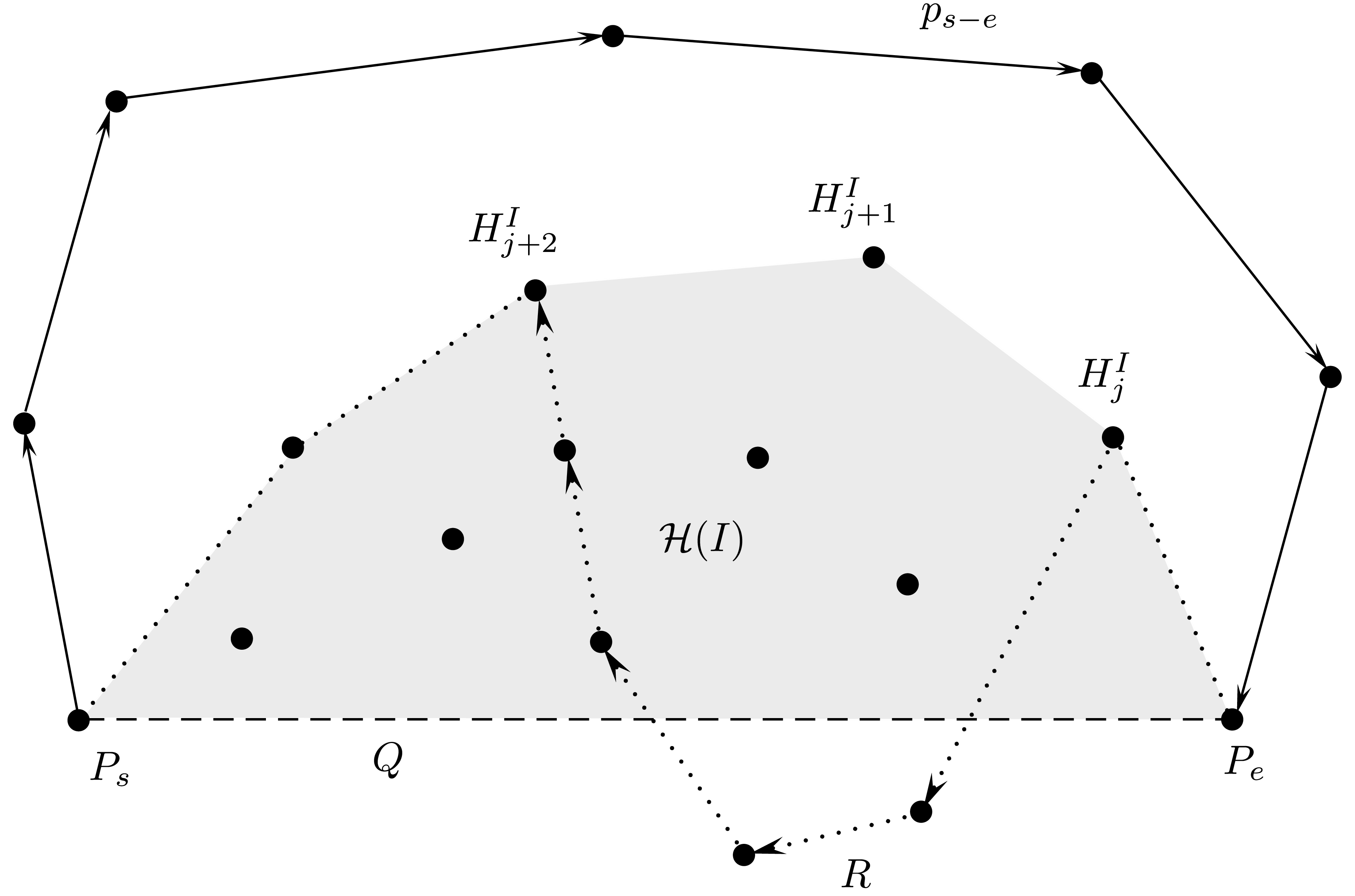
 ps−e
 Q
 ps−e
 PePs¯
 I
 Q
 Ps
 Pe
 H(I)
 R
 ps−e
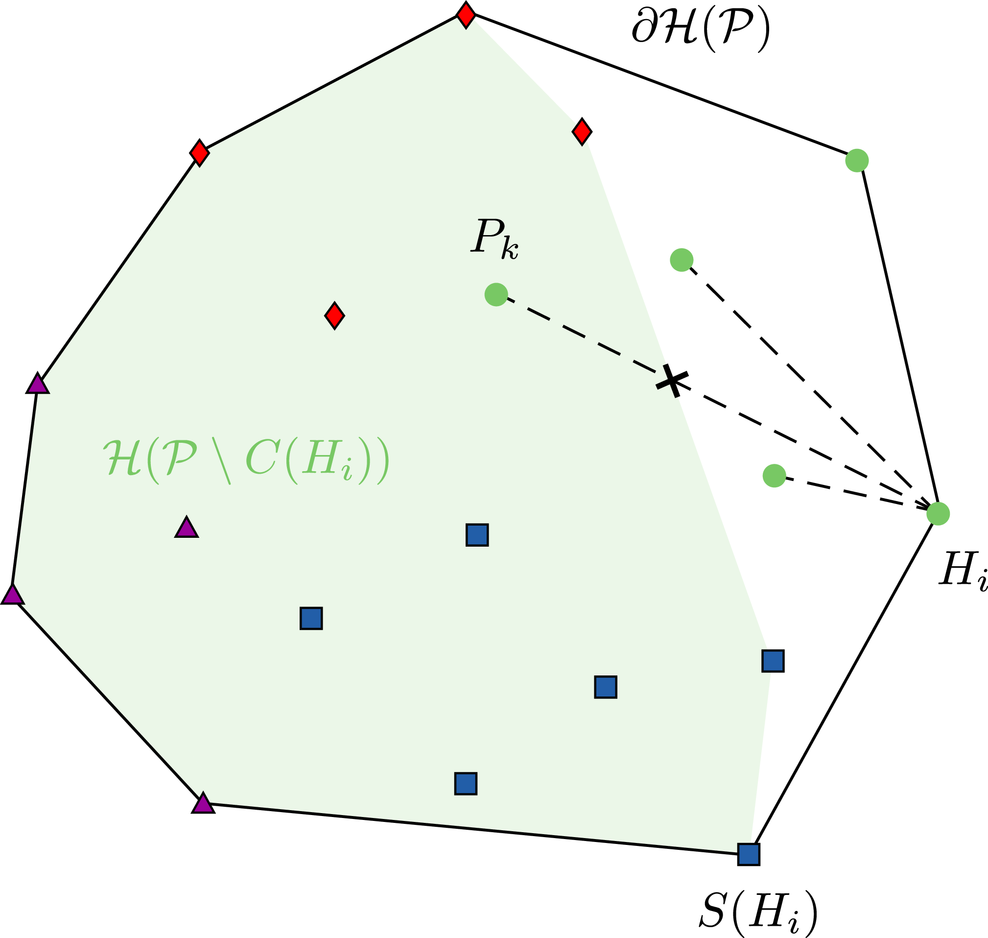
 Pk
 Hi
 HiPk¯
 H(P∖C(Hi))
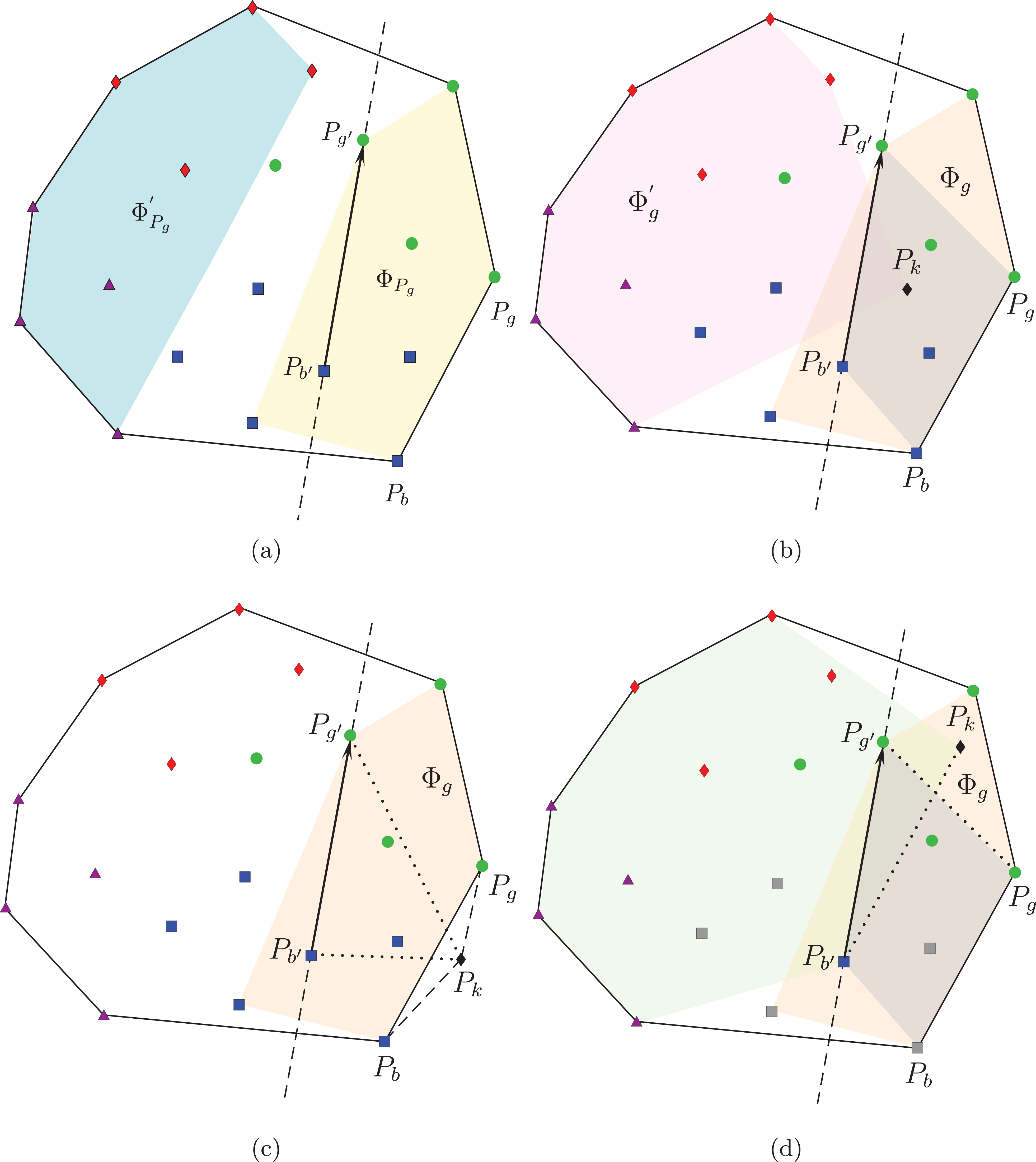
 Pb′
 Pg′
 ΦPg∩ΦPg′=∅
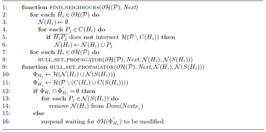
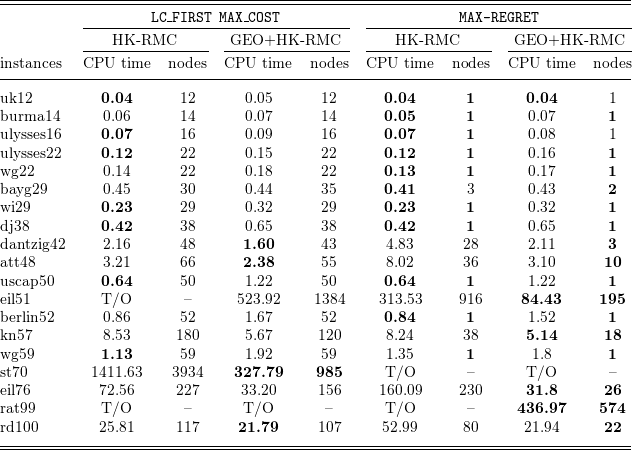
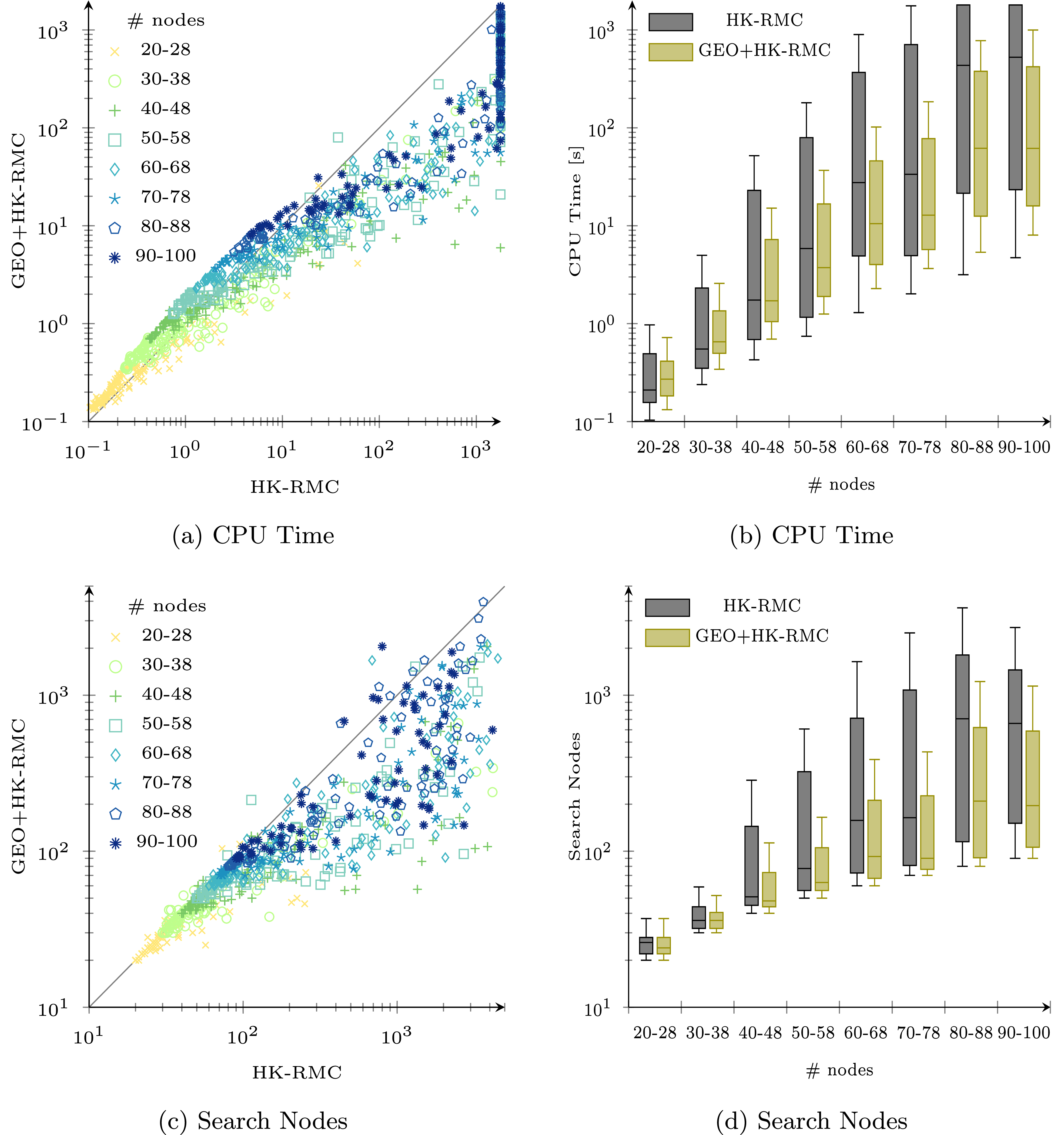
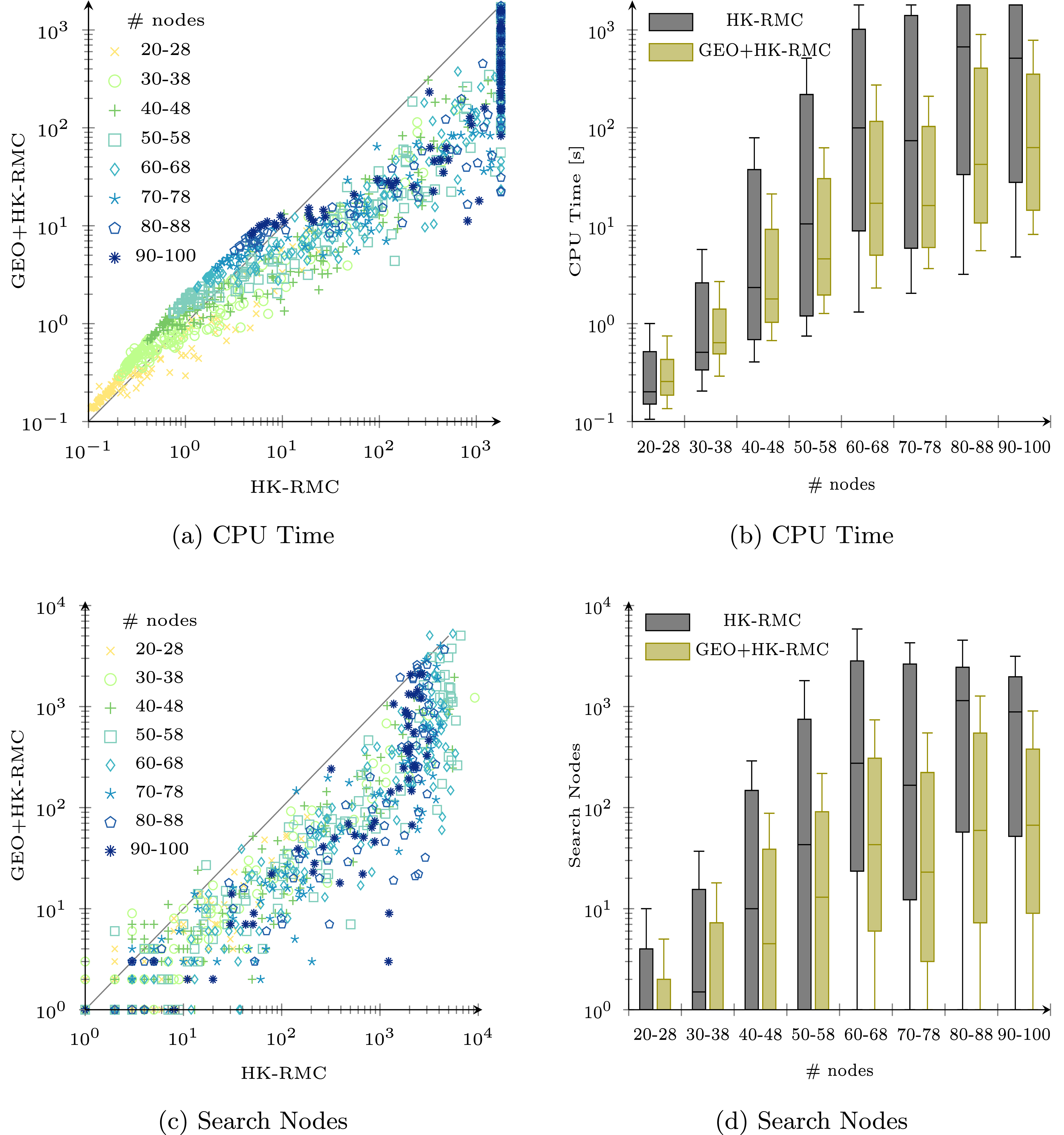
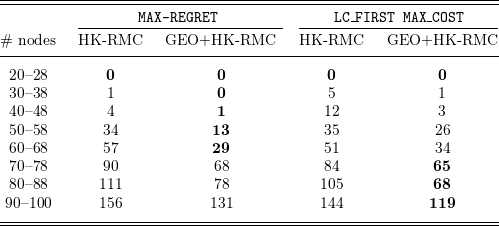
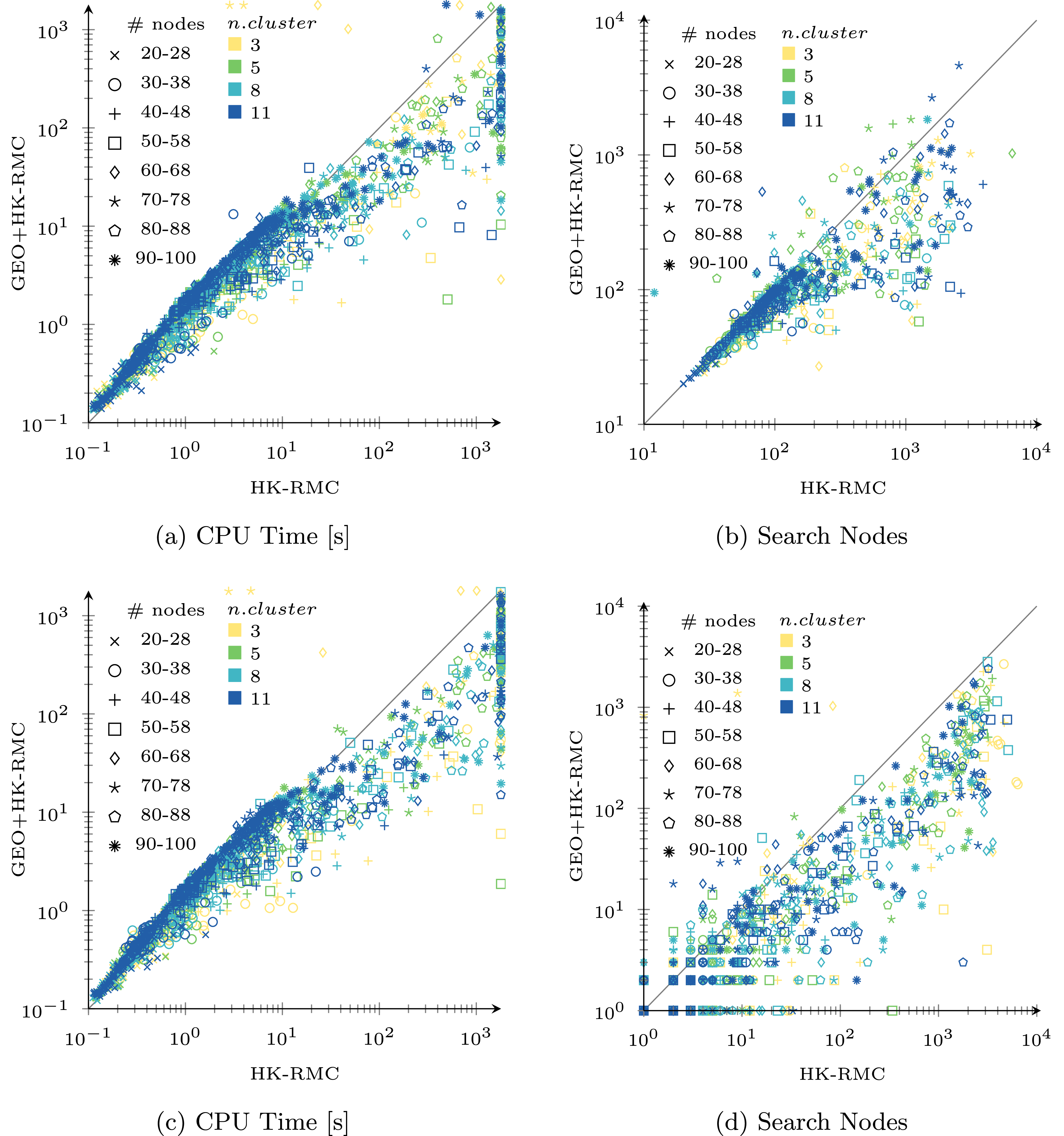
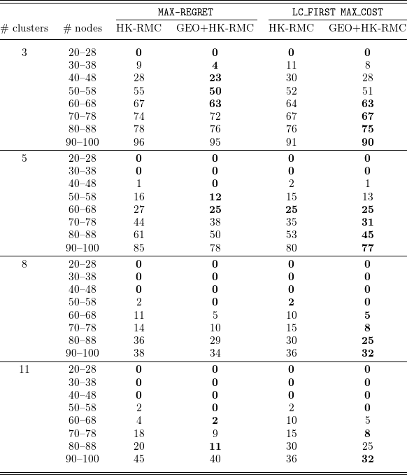
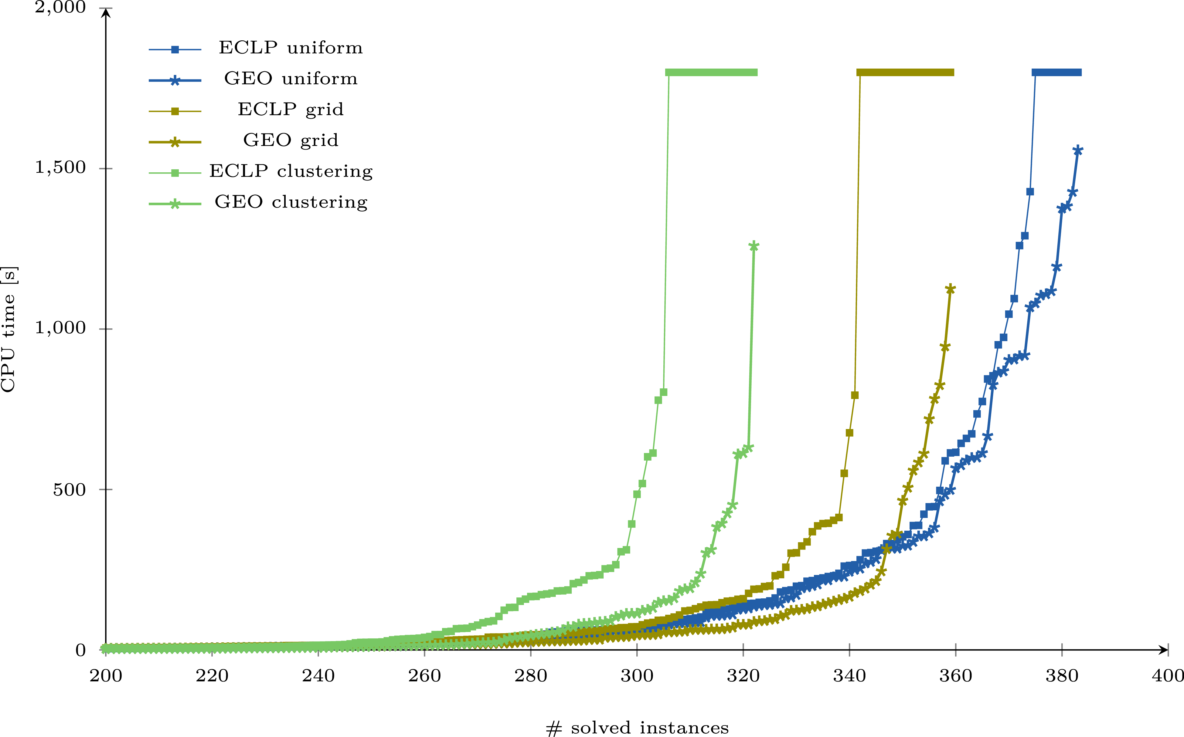

 Open access

