Secondary instabilities of Görtler vortices in high-speed boundary layer flows

Jie Ren; Song Fu

doi:10.1017/jfm.2015.490

Secondary instabilities of Görtler vortices in high-speed boundary layer flows

Published online by Cambridge University Press: 21 September 2015

Jie Ren and

Song Fu

Show author details

Jie Ren: Affiliation:
School of Aerospace Engineering, Tsinghua University, Beijing, 100084, China
Song Fu*: Affiliation:
School of Aerospace Engineering, Tsinghua University, Beijing, 100084, China
*: †Email address for correspondence: fs-dem@tsinghua.edu.cn

Article contents

Abstract
Introduction
Formulation of the problem
Spatial development of Görtler vortices
The secondary instability
Conclusions
References

Rights & Permissions

Abstract

Görtler vortices developed in laminar boundary layer experience remarkable changes when the flow is subjected to compressibility effects. In the present study, five $\mathit{Ma}$ numbers, covering incompressible to hypersonic flows, at $\mathit{Ma}=0.015$ , 1.5, 3.0, 4.5 and 6.0 are specified to illustrate these effects. Görtler vortices in subsonic and moderate supersonic flows ( $\mathit{Ma}=0.015$ , 1.5 and 3.0) are governed by the conventional wall-layer mode (mode W). In hypersonic flows ( $\mathit{Ma}=4.5$ , 6.0), the trapped-layer mode (mode T) becomes dominant. This difference is maintained and intensifies downstream leading to different scenarios of secondary instabilities. The linear and nonlinear development of Görtler vortices which are governed by dominant modal disturbances are investigated with direct marching of the nonlinear parabolic equations. The secondary instabilities of Görtler vortices set in when the resulting streaks are adequately developed. They are studied with Floquet theory at multiple streamwise locations. The secondary perturbations become unstable downstream following the sequence of sinuous mode type I, varicose mode and sinuous mode type II, indicating an increasing threshold amplitude. Onset conditions are determined for these modes. The above three modes can each have the largest growth rate under the right conditions. In the hypersonic cases, the threshold amplitude $A(u)$ is dramatically reduced, showing the significant impact of the thermal streaks. To investigate the parametric effect of the spanwise wavenumber, three global wavenumbers ( $B=0.5$ , 1.0 and $2.0\times 10^{-3}$ ) are specified. The relationship between the dominant mode (sinuous or varicose) and the spanwise wavenumber of Görtler vortices found in incompressible flows (Li & Malik, J. Fluid Mech., vol. 297, 1995, pp. 77–100) is shown to be not fully applicable in high-speed cases. The sinuous mode becomes the most dangerous, regardless of the spanwise wavelength when $\mathit{Ma}>3.0$ . The subharmonic type can be the most dangerous mode while the detuned type can be neglected, although some of the sub-dominant secondary modes reach their peak growth rates under detuned states.

JFM classification

Instability: Absolute/convective instability Compressible Flows: Compressible boundary layers Instability: Nonlinear instability

Information

Type: Papers
Information: Journal of Fluid Mechanics , Volume 781 , 25 October 2015, pp. 388 - 421
DOI: https://doi.org/10.1017/jfm.2015.490 [Opens in a new window]
Copyright: © 2015 Cambridge University Press

1. Introduction

Görtler instability (Görtler Reference Görtler1940), the centrifugal instability of a boundary layer over a concave wall, arises due to the imbalance between the centrifugal force and the wall-normal pressure gradient. Streamwise-oriented, counter-rotating vortices (Görtler vortices) are consequently generated, maintained and can be significantly intensified downstream promoting flow transition. Most of early studies were conducted within the framework of incompressible flows (see reviews by Herbert Reference Herbert1976; Hall Reference Hall1990; Floryan Reference Floryan1991; Saric Reference Saric1994, and the recent research by Wu, Zhao & Luo (Reference Wu, Zhao and Luo2011)).

Görtler instabilities have been formerly studied with normal mode analysis locally in order to obtain the so-called neutral curve (see Herbert Reference Herbert1976). The parallel flow assumption was often adopted. In fact, Görtler instabilities exhibit crucial differences compared to conventional Tollmien–Schlichting (T–S) waves. Görtler instability is governed by parabolic equations (see Hall Reference Hall1990). The initial conditions and the non-parallel nature of the boundary layer can exert a critical influence. Therefore, a unique neutral curve is no longer tenable (Hall Reference Hall1982, Reference Hall1983). The recent study by Wu et al. (Reference Wu, Zhao and Luo2011) has fully uncovered the different regimes of the excitation and spatial development of Görtler vortices. Local normal mode analysis is mathematically justified when the streamwise coordinate is large enough (where the inviscid regime is reached). From a numerical point of view, the eigenvalue problem (EVP) is valid only when the Görtler number $G=\mathit{Re}\sqrt{{\it\delta}_{x}^{\ast }/R^{\ast }}$ is large. Here $\mathit{Re}$ is based on the local boundary layer length scale ${\it\delta}_{x}^{\ast }=\sqrt{{\it\nu}_{\infty }^{\ast }x^{\ast }/U_{\infty }^{\ast }}$ , $R^{\ast }$ is the local radius of curvature and $x^{\ast }$ is the streamwise coordinate. The asterisk denotes any dimensional quantities hereafter. Typically, $G>7$ is satisfactory for applying the normal mode approach (Bottaro & Luchini Reference Bottaro and Luchini1999). Discussions on the validity of the local EVP can also be found in Day, Herbert & Saric (Reference Day, Herbert and Saric1990) and Goulpié, Klingmann & Bottaro (Reference Goulpié, Klingmann and Bottaro1996). Similar restrictions exist for compressible flows with $O(1)~\mathit{Ma}$ number (see Hall & Fu Reference Hall and Fu1989; Spall & Malik Reference Spall and Malik1989).

Görtler instability, by itself, does not lead to flow transition. Instead, low- and high-speed streaks are produced and enhanced by persistent streamwise counter-rotating vortices (termed Görtler vortices or Görtler rolls). Besides the Görtler flow, streaks can form in a laminar boundary layer in other situations through the lift-up mechanism (Ellingsen & Palm Reference Ellingsen and Palm1975; Landahl Reference Landahl1975, Reference Landahl1980). For instance, streaks develop due to the transient growth of optimal disturbances (Hultgren & Gustavsson Reference Hultgren and Gustavsson1981; Andersson, Berggren & Henningson Reference Andersson, Berggren and Henningson1999; Luchini Reference Luchini2000) which are not necessarily physically realizable perturbations. Streaks can be generated by free stream turbulence (FST) and this was analysed by Leib, Wundrow & Goldstein (Reference Leib, Wundrow and Goldstein1999) and Ricco & Wu (Reference Ricco and Wu2007). Streaks may also be generated by roughness elements of the right size (Morkovin Reference Morkovin, Hussaini and Voigt1990; Joslin & Grosch Reference Joslin and Grosch1995; Tumin & Reshotko Reference Tumin and Reshotko2005). Counterparts of the above mechanisms were also observed in compressible flows (see, for example, Hanifi, Schmid & Henningson Reference Hanifi, Schmid and Henningson1996; Tumin & Reshotko Reference Tumin and Reshotko2001, Reference Tumin and Reshotko2003; De Tullio et al. Reference De Tullio, Paredes, Sandham and Theofilis2013). These flows thus share many similarities. The secondary instability of streaks has been recognized as a key factor leading the boundary layer to transition. The subsequent breakdown process is observed to proceed rather rapidly (Swearingen & Blackwelder Reference Swearingen and Blackwelder1987). Studying the secondary instability is thus important to understand the physical mechanism of the transition process. A number of numerical investigations (see Hall & Horseman Reference Hall and Horseman1991; Sabry & Liu Reference Sabry and Liu1991; Yu & Liu Reference Yu and Liu1991, Reference Yu and Liu1994; Liu & Domaradzki Reference Liu and Domaradzki1993; Li & Malik Reference Li and Malik1995; Park & Huerre Reference Park and Huerre1995; Bottaro & Klingmann Reference Bottaro and Klingmann1996) were carried out using parameters taken from experiment (Swearingen & Blackwelder Reference Swearingen and Blackwelder1987). Identifying the most dangerous secondary mode is of fundamental importance as it determines both the scenario and location of transition. For incompressible Görtler flow, the sinuous and varicose modes are found (Hall & Horseman Reference Hall and Horseman1991; Yu & Liu Reference Yu and Liu1991) and analysed with energy balancing mechanisms (Liu & Domaradzki Reference Liu and Domaradzki1993; Yu & Liu Reference Yu and Liu1994; Park & Huerre Reference Park and Huerre1995). Schrader, Brandt & Zaki (Reference Schrader, Brandt and Zaki2011) performed the first spatial DNS for a Görtler flow including the experimental conditions of Tandiono, Winoto & Shah (Reference Tandiono, Winoto and Shah2008), Tandiono, Winoto & Shah (Reference Tandiono, Winoto and Shah2009) for incompressible flows. In the breakdown process reported, both the sinuous and varicose modes were observed. It was found that the sinuous mode appeared first and required a lower amplitude of the streak (see Bottaro & Klingmann Reference Bottaro and Klingmann1996; Andersson et al. Reference Andersson, Brandt, Bottaro and Henningson2001) while varicose modes were stronger for large wavelengths of Görtler vortices (Li & Malik Reference Li and Malik1995). This was later verified in an experiment for the secondary instability of streaks along a flat plate (Asai, Minagawa & Nishioka Reference Asai, Minagawa and Nishioka2002). In the study of Li & Malik (Reference Li and Malik1995), the subharmonic type was also highlighted as they had comparable growth rate to the fundamental counterparts. Among these studies, a particular sinuous mode had been missed out. This mode is sinuous in nature but its disturbances are distributed near the stem of the mushroom (see Ren & Fu Reference Ren and Fu2014b , p. 560, figure 6d). In the wake of an isolated roughness element, this type of mode (which is not the most dangerous) was also reported (see the Bi-global analysis of De Tullio et al. Reference De Tullio, Paredes, Sandham and Theofilis2013). In the current study, we shall show this mode can have the largest growth rate and is therefore responsible for the sinuous breakdown under certain conditions.

Concerning the receptivity problem (see Hall Reference Hall1990; Bassom & Seddougui Reference Bassom and Seddougui1995, for early reviews), Görtler vortices can be excited through surface roughness (Denier, Hall & Seddougui Reference Denier, Hall and Seddougui1991; Bassom & Hall Reference Bassom and Hall1994; Luchini & Bottaro Reference Luchini and Bottaro1998; Schrader et al. Reference Schrader, Brandt and Zaki2011) or/and FST (Luchini & Bottaro Reference Luchini and Bottaro1998; Schrader et al. Reference Schrader, Brandt and Zaki2011; Wu et al. Reference Wu, Zhao and Luo2011). A recent study indicates that zero or low-frequency free stream vortices most effectively excite the Görtler vortices (Schrader et al. Reference Schrader, Brandt and Zaki2011). In previous DNS studies, (see Schrader et al. Reference Schrader, Brandt and Zaki2011, for example), FST and the inlet condition were often represented by continuous spectrum of the O-S/Squire equations, such a practice was questioned by Dong & Wu (Reference Dong and Wu2013), who showed that continuous modes do not represent FST or its entrainment into the boundary layer. More recently, Sescu & Thompson (Reference Sescu and Thompson2015) revealed the influence of the roughness geometry on the excitation, development and secondary instability of Görtler vortices.

For hypersonic Görtler flows, the most significant flow feature is the existence of the temperature adjustment layer near the upper edge of the boundary layer, which gives rise to the trapped-layer mode (mode T disturbances rest in the layer near the upper edge of boundary layer) (Fu & Hall Reference Fu and Hall1992, Reference Fu and Hall1993). This mode becomes the most dangerous when the $\mathit{Ma}$ number is larger than a critical value, e.g. $\mathit{Ma}\geqslant 4$ , approximately. The mode T can also intersect with the conventional wall-layer mode (mode W disturbances exist in the layer close to the wall) at very large $\mathit{Re}$ numbers. The crossover of the growth rate between the two modes has been studied with the asymptotic (Dando & Seddougui Reference Dando and Seddougui1993) and the local & marching methods (Ren & Fu Reference Ren and Fu2014a ). Recently, Ren & Fu (Reference Ren and Fu2015) studied the discrete spectrum in a $\mathit{Ma}=4.5$ flow, highlighting the possible synchronizations for Görtler modes.

Experimental studies of Görtler vortices in high-speed flows are scarce. The $\mathit{Ma}=7$ experiment by Luca et al. (Reference Luca, Cardone, Aymer de la Chevalerie and Fonteneau1993) demonstrated the generation of Görtler vortices from spanwise periodic temperature variations. The wavelength was found to maintain a constant value along the streamwise direction. However, neither the base flow nor perturbation quantities were reported in the experiment. Other experiments were conducted over a compression ramp (de la Chevalerie et al. Reference de la Chevalerie, Fonteneau, Luca and Cardone1997; Schrijer Reference Schrijer2010). Due to the concave curvature of the streamlines in the region of the flow separation, the Görtler mechanism is engaged. However, properly handling the Görtler instability is of vital importance in the design of high-speed wind tunnel nozzles (Chen, Wilkinson & Beckwith Reference Chen, Wilkinson and Beckwith1993; Schneider Reference Schneider1998, Reference Schneider2008).

Discussions on the secondary instability of Görtler vortices in compressible flows can be found in Fu & Hall (Reference Fu and Hall1992), Whang & Zhong (Reference Whang and Zhong2001) and Li et al. (Reference Li, Choudhari, Chang, Wu and Greene2010). In the numerical study by Whang & Zhong (Reference Whang and Zhong2001), a $\mathit{Ma}=15$ flow with a concave surface was simulated with DNS. The varicose mode which develops into the horseshoe vortex was found to be dominant over the sinuous mode. In the $\mathit{Ma}=6$ study by Li et al. (Reference Li, Choudhari, Chang, Wu and Greene2010), however, the most dangerous mode was demonstrated to be the sinuous mode. Besides the secondary instability of Görtler vortices, the other routes towards transition, e.g. the Görtler–Mack mode interactions, were also explored (Li et al. Reference Li, Choudhari, Chang, Wu and Greene2010).

Taking a broad view of existing studies in compressible Görtler flows, however, we note that many aspects related to the secondary instabilities of Görtler vortices remain unclear. For example, what is the effect of increasing $\mathit{Ma}$ number on the secondary instability with the mode T being the governing mode? How is the threshold amplitude (Andersson et al. Reference Andersson, Brandt, Bottaro and Henningson2001) influenced by the Mach number? Is the relationship between the growth rate of the varicose/sinuous mode and the basic wavelength of Görtler vortices (Li & Malik Reference Li and Malik1995) still valid in compressible flows? Should the subharmonic and detuned secondary instabilities be responsible for the transition process? The present study attempts to investigate, comprehensively the secondary instabilities of compressible Görtler vortices in order to answer these questions.

In § 2, the mathematical formulation of the secondary instability and the definition of the global parameters are provided. The linear and nonlinear spatial development of Görtler vortices are discussed in § 3. Results for the fundamental, subharmonic and detuned secondary instabilities of Görtler vortices are presented and discussed in § 4. Further discussions are provided and the present study is concluded with § 5.

2. Formulation of the problem

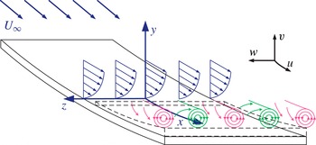
In the coordinates defined in figure 1, the flow is governed by the compressible Navier–Stokes (N–S) equations. Axes $x$ , $y$ and $z$ are along streamwise, wall-normal and spanwise directions, respectively. The corresponding Lamé coefficients are $h_{1}=1+ky$ , $h_{2}=h_{3}=1$ with $k$ representing the streamwise curvature (negative). The coordinates are scaled with the boundary layer length scale ${\it\delta}_{0}^{\ast }$ at the inlet of the flow, e.g. $x=x^{\ast }/{\it\delta}_{0}^{\ast }=x^{\ast }/\sqrt{{\it\nu}_{\infty }^{\ast }x_{0}^{\ast }/U_{\infty }^{\ast }}$ . All flow quantities are scaled with their free stream values except the pressure which is scaled by ${\it\rho}_{\infty }^{\ast }(U_{\infty }^{\ast })^{2}$ . The dimensionless form of the Navier–Stokes equations are thus characterized with the dimensionless numbers:

(2.1a−c )

$$\begin{eqnarray}\mathit{Re}_{0}={\displaystyle \frac{{\it\rho}_{\infty }^{\ast }U_{\infty }^{\ast }{\it\delta}_{0}^{\ast }}{{\it\mu}_{\infty }^{\ast }}},\quad \mathit{Ma}={\displaystyle \frac{U_{\infty }^{\ast }}{\sqrt{{\it\gamma}R_{air}^{\ast }T_{\infty }^{\ast }}}},\quad \mathit{Pr}={\displaystyle \frac{{\it\mu}_{\infty }^{\ast }C_{p}^{\ast }}{{\it\kappa}_{\infty }^{\ast }}}.\end{eqnarray}$$

The disturbance $\tilde{\boldsymbol{q}}=(\tilde{{\it\rho}},\tilde{u} ,\tilde{v},\tilde{w},\tilde{T})^{\text{T}}$ is governed by nonlinear stability equations. The governing equation is derived from compressible Navier–Stokes equations by introducing disturbances to the laminar flow $\boldsymbol{q}(x,y,z,t)=\boldsymbol{q}_{0}(x,y)+\tilde{\boldsymbol{q}}(x,y,z,t)$ and subtracting the basic flow relations. The disturbances are then expressed with Fourier series

(2.2)

$$\begin{eqnarray}\tilde{\boldsymbol{q}}(x,y,z,t)=\mathop{\sum }_{m=-M}^{M}\mathop{\sum }_{n=-N}^{N}\hat{\boldsymbol{q}}_{mn}(x,y)\exp (\text{i}n{\it\beta}z-\text{i}m{\it\omega}t).\end{eqnarray}$$

In compact form, the stability equations can be written as

(2.3)

$$\begin{eqnarray}\mathbf{\mathscr{L}}_{0}\hat{\boldsymbol{q}}_{mn}+\mathbf{\mathscr{L}}_{1}{\displaystyle \frac{\partial \hat{\boldsymbol{q}}_{mn}}{\partial x}}+\mathbf{\mathscr{L}}_{2}{\displaystyle \frac{\partial \hat{\boldsymbol{q}}_{mn}}{\partial y}}+\mathbf{\mathscr{L}}_{3}{\displaystyle \frac{\partial ^{2}\hat{\boldsymbol{q}}_{mn}}{\partial x^{2}}}+\mathbf{\mathscr{L}}_{4}{\displaystyle \frac{\partial ^{2}\hat{\boldsymbol{q}}_{mn}}{\partial x\partial y}}+\mathbf{\mathscr{L}}_{5}{\displaystyle \frac{\partial ^{2}\hat{\boldsymbol{q}}_{mn}}{\partial y^{2}}}+\hat{\boldsymbol{N}}_{mn}=0.\end{eqnarray}$$

The operators $\mathbf{\mathscr{L}}_{0},\mathbf{\mathscr{L}}_{1},\ldots ,\mathbf{\mathscr{L}}_{5}$ in (2.3) are functions of $\mathit{Re}_{0}$ , $\mathit{Ma}$ , $\mathit{Pr}$ , $n{\it\beta}$ , $m{\it\omega}$ , $k$ and basic flows (see appendix A for detailed expressions of these operators). The vector $\hat{\boldsymbol{N}}_{mn}$ stands for nonlinear terms. Sutherland’s law and Stoke’s hypothesis are applied for closure of the N–S equations. The fluid is assumed to be calorically perfect gas with $\mathit{Pr}$ number being constant. Typically, $\mathit{Pr}=0.72$ is specified in this study. An adiabatic wall is considered with a stagnation temperature of $T_{s}^{\ast }=300~\text{K}$ . It can be inferred from (2.3) that the four leading curvature terms are ${\it\rho}k/h_{1}$ in $\mathbf{\mathscr{L}}_{0}(1,3)$ , ${\it\rho}uk/h_{1}$ in $\mathbf{\mathscr{L}}_{0}(2,3)$ , $-u^{2}k/h_{1}$ in $\mathbf{\mathscr{L}}_{0}(3,1)$ and $-2{\it\rho}uk/h_{1}$ in $\mathbf{\mathscr{L}}_{0}(3,2)$ . The curvature is coupled with the basic flows and acts on the zeroth-order derivative operator $\mathbf{\mathscr{L}}_{0}$ . The basic flows here are specified as the self-similar solution of the compressible boundary layer.

Figure 1.

Sketch of the counter-rotating Görtler vortices encountered on a slightly concave wall. The orthogonal curvilinear coordinates $x$ , $y$ and $z$ denote streamwise, wall-normal and spanwise directions. Velocity components $u$ , $v$ and $w$ are defined in the directions shown. The near wall area (dashed lines) indicates the undisturbed region due to the dominance of trapped-layer modes (mode T) in hypersonic boundary layers.

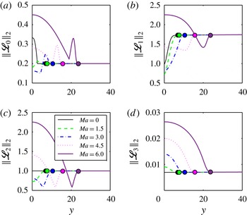
Going through the stability equations (2.3), one observes that the $\mathit{Ma}$ number, representing the compressibility effect, plays an important role in the operator $\mathbf{\mathscr{L}}_{i}$ . To evaluate the $\mathit{Ma}$ number effect, the two-norm of the operators in (2.3) are plotted in figure 2 with representative parameters. The two-norm $\Vert \mathbf{\mathscr{L}}_{i}\Vert _{2}={\it\sigma}_{max}(\mathbf{\mathscr{L}}_{i})$ corresponds to the largest singular value of the matrix and measures the amplitude of the operator. In figure 2, we have $\mathit{Re}_{0}=200$ , local curvature $k=-2\times 10^{-4}$ , spanwise wavenumber ${\it\beta}=0.2$ , angular frequency ${\it\omega}=0$ and $m=n=1$ . The zeroth and first-order derivative terms $\mathbf{\mathscr{L}}_{0}$ , $\mathbf{\mathscr{L}}_{1}$ and $\mathbf{\mathscr{L}}_{2}$ are of the order of $O(1)$ . As shown in the figure, when $\mathit{Ma}$ is increased, $\Vert \mathbf{\mathscr{L}}_{0}\Vert _{2}$ , $\Vert \mathbf{\mathscr{L}}_{1}\Vert _{2}$ and $\Vert \mathbf{\mathscr{L}}_{2}\Vert _{2}$ decrease first but then increase near the wall. Meanwhile, a second peak is observed near the edge of the boundary layer. The operators then act as constants outside the boundary layer. The second-order derivative operators $\mathbf{\mathscr{L}}_{3}$ , $\mathbf{\mathscr{L}}_{4}$ and $\mathbf{\mathscr{L}}_{5}$ have simple expressions as can be seen in appendix A and are derived from the viscous terms of the N–S equations. The order of these operators are of $O(1/\mathit{Re})$ , small enough to be neglected except for the term which is related to $\mathbf{\mathscr{L}}_{5}$ for the second-derivative in the wall-normal direction. This is consistent with the fact that Görtler vortices develop along the streamwise direction as slowly as the boundary layer does. The stability equations (2.3), hence, can be parabolized by dropping $\mathbf{\mathscr{L}}_{3}$ and $\mathbf{\mathscr{L}}_{4}$ .

Figure 2.

Two-norm of the operators $\Vert \mathbf{\mathscr{L}}_{0}\Vert _{2}$ , $\Vert \mathbf{\mathscr{L}}_{1}\Vert _{2}$ , $\Vert \mathbf{\mathscr{L}}_{2}\Vert _{2}$ and $\Vert \mathbf{\mathscr{L}}_{3}\Vert _{2}$ of the stability equations (2.3) as a function of the wall-normal coordinate. $\mathit{Re}_{0}=200$ , $k=-2\times 10^{-4}$ , ${\it\beta}=0.2$ , ${\it\omega}=0$ , $m=n=1$ , $\mathit{Ma}=0.015$ , 1.5, 3.0, 4.5 and 6.0. The solid circles show the upper edge of the boundary layer defined as 99.99 % of the freestream velocity.

The nonlinear development of Görtler vortices are integrated up to a (quasi-) saturated status. The fully developed Görtler vortices then act as the base flow for secondary stability analysis. The readers may refer to Li & Malik (Reference Li and Malik1995), Li et al. (Reference Li, Choudhari, Duan and Chang2014), Ren & Fu (Reference Ren and Fu2014a ) for details of the nonlinear marching of the basic states and validations.

In the methodology of the linear secondary instability (Herbert Reference Herbert1988; Schmid & Henningson Reference Schmid and Henningson2001), the stability analysis is performed typically in a $y{-}z$ cross-section (so-called Bi-global). The disturbances, therefore, are assumed to be inhomogeneous in the wall-normal and spanwise direction but periodic in time and streamwise direction, i.e.

(2.4)

$$\begin{eqnarray}\left.\begin{array}{@{}c@{}}\displaystyle \tilde{q}_{s}(x,y,z,t)=\text{e}^{{\it\gamma}z}\text{e}^{{\it\omega}_{s}t+\text{i}{\it\alpha}_{s}x}\mathop{\sum }_{m=-\infty }^{\infty }\hat{q}_{m}(y)\text{e}^{\text{i}m{\it\beta}z}\\ 0\leqslant {\it\gamma}_{i}\leqslant \displaystyle \frac{{\it\beta}}{2}.\end{array}\right\}\end{eqnarray}$$

Here, $\tilde{q}_{s}=(\tilde{{\it\rho}}_{s},\tilde{u} _{s},\tilde{v}_{s},\tilde{w}_{s},\tilde{T}_{s})^{\text{T}}$ is the secondary disturbance on Görtler vortices and ${\it\beta}$ is the spanwise wavenumber of the primary Görtler mode. The subscript $s$ indicates the quantities with respect to secondary instabilities. In the temporal analysis considered here, the streamwise wavenumber ${\it\alpha}_{s}$ is specified and the angular frequency ${\it\omega}_{s}$ is the eigenvalue to be determined. The Floquet parameter ${\it\gamma}$ decides the type of the secondary instability and ${\it\gamma}_{i}/{\it\beta}\in [0,0.5]$ . ${\it\gamma}_{i}/{\it\beta}=0$ produces the fundamental, ${\it\gamma}_{i}/{\it\beta}=0.5$ the subharmonic and the other values result in detuned types. The periodic base flow at a specified streamwise location is written as

(2.5)

$$\begin{eqnarray}Q(y,z)=\bar{q}_{0}(y)+\mathop{\sum }_{n=-\infty }^{\infty }\bar{Q}_{n}(y)\text{e}^{\text{i}n{\it\beta}z}.\end{eqnarray}$$

Substituting (2.4) and (2.5) into the N–S equations, the secondary instability equation finally reduces to the EVP, i.e.

(2.6)

$$\begin{eqnarray}\mathbf{\mathscr{L}}{\it\Theta}={\it\omega}_{s}\mathbf{\mathscr{R}}{\it\Theta}.\end{eqnarray}$$

The EVP is numerically solved with the Chebyshev and Fourier collocation methods in the $y$ and $z$ directions, respectively. The dimension of the sparse matrix $\mathbf{\mathscr{L}}$ and $\mathbf{\mathscr{R}}$ is $(N_{s}\times N_{s})$ with $N_{s}=5N_{y}\cdot N_{z}$ . Here $N_{y}$ is the number of points in the wall-normal direction and $N_{z}$ is the number of the Fourier components. The Arnoldi method is applied for shooting the targeted eigenvalues.

Before the discussion of results, the global stability parameters are defined first. They are also recommended for future studies of the stability problem. In conventional stability analysis, the concept of the local normal mode analysis assumes a simple wave-like disturbance $\tilde{q}(x,y,z,t)=\hat{q}(y)\exp [\text{i}({\it\alpha}x+{\it\beta}z-{\it\omega}t)]$ (Mack Reference Mack1975), thus, the wavenumber ${\it\alpha},{\it\beta}$ and the angular frequency ${\it\omega}$ are introduced. However, these local variables are scaled with the boundary layer thickness which is a variable itself. This is an inconvenience when the marching or global method is applied. As a result, the dimensionless frequency $F$ is often employed, e.g. in Ma & Zhong (Reference Ma and Zhong2003)

(2.7)

$$\begin{eqnarray}F=\frac{{\it\omega}^{\ast }{\it\nu}_{\infty }^{\ast }}{U_{\infty }^{\ast 2}}=\frac{{\it\omega}}{\mathit{Re}}.\end{eqnarray}$$

Here $\mathit{Re}=\sqrt{{\it\rho}_{\infty }^{\ast }U_{\infty }^{\ast }x^{\ast }/{\it\mu}_{\infty }^{\ast }}$ represents the local Reynolds number which scales with $\sqrt{x^{\ast }}$ . This will be used in the present study as a measure of the streamwise coordinate. The dimensionless frequency $F$ corresponds to a physical frequency free from the streamwise coordinate. In this study, $F$ is termed the global frequency. Similarly, the global wavenumber $B$ and the global streamwise curvature $K$ are also defined as

(2.8)

$$\begin{eqnarray}\displaystyle & B=\displaystyle \frac{2{\rm\pi}{\it\nu}_{\infty }^{\ast }}{U_{\infty }^{\ast }{\it\lambda}^{\ast }}=\displaystyle \frac{{\it\beta}}{\mathit{Re}}, & \displaystyle\end{eqnarray}$$

(2.9)

$$\begin{eqnarray}\displaystyle & K=-\displaystyle \frac{{\it\nu}_{\infty }^{\ast }}{U_{\infty }^{\ast }R^{\ast }}=\displaystyle \frac{k}{\mathit{Re}}. & \displaystyle\end{eqnarray}$$

$B$ and

$K$ thus reflect the physical wavelength

${\it\lambda}^{\ast }$ and radius of curvature

$R^{\ast }$ . They are related to the wavelength parameter of Görtler vortices (see Saric 1994, for example)

(2.10)

$$\begin{eqnarray}{\it\Lambda}=\frac{U_{\infty }^{\ast }{\it\lambda}^{\ast }}{{\it\nu}_{\infty }^{\ast }}\sqrt{\frac{{\it\lambda}^{\ast }}{R^{\ast }}}=\sqrt{\left(\frac{2{\rm\pi}}{B}\right)^{3}(-K)}.\end{eqnarray}$$

3. Spatial development of Görtler vortices

3.1. Görtler modes from the local normal mode analysis

As the steady state for secondary instabilities to appear the linear and nonlinear development of Görtler vortices are discussed in this section. To investigate the effect of the $\mathit{Ma}$ number on the secondary instability of Görtler vortices, five groups of cases are studies here with $\mathit{Ma}=0.015$ , 1.5, 3.0, 4.5 and 6.0. The $\mathit{Ma}=0.015$ case represents the incompressible flow and coincides with the experimental conditions of Swearingen & Blackwelder (Reference Swearingen and Blackwelder1987). The $\mathit{Ma}=1.5$ and 3.0 cases are for moderate supersonic flows, while $\mathit{Ma}=4.5$ and 6.0 are for hypersonic flows. For each $\mathit{Ma}$ number, a number of cases with different combinations of wavenumbers $B$ and Floquet parameters ${\it\gamma}$ are considered to study the effect of the spanwise wavelength and the tuning parameter. These cases share the following flow parameters: global curvature $K=-10^{-6}$ , Reynolds number $\mathit{Re}\in [200,1000]$ and thus Görtler number $G\in [2.8,31.6]$ . The global curvature is chosen to represent the most commonly engaged Görtler flows. 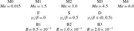Recall that in the experiments of Swearingen & Blackwelder (Reference Swearingen and Blackwelder1987) and Mitsudharmadi, Winoto & Shah (Reference Mitsudharmadi, Winoto and Shah2005), $K=-0.94\times 10^{-6}$ and $-2.5\times 10^{-6}$ , respectively. The flow parameters of all the cases are listed in table 1. For example, the case M3-S-B2 indicates the flow with Mach number $\mathit{Ma}=4.5$ , Floquet parameter ${\it\gamma}_{i}/{\it\beta}=0.5$ (subharmonic) and global wavenumber $B=1.0\times 10^{-3}$ .

Table 1.

Parameters of the flow cases in the current study. The five Mach numbers increase linearly from incompressible to hypersonic conditions. The three global spanwise wavenumbers cover the (quasi-) most amplified Görtler modes in all the five Mach numbers. In the incompressible case, these wavenumbers coincide with the wavelengths 36, 18 and 9 mm considered in Li & Malik (Reference Li and Malik1995).

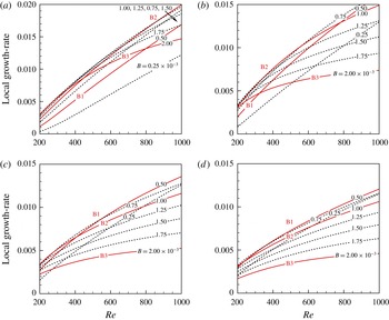
In figure 3, the local growth rate of the primary Görtler modes as a function of $\mathit{Re}$ is given for the supersonic cases. Only the most amplified mode is plotted here apart from the other sub-dominant Görtler modes. The local normal mode analysis is performed within $\mathit{Re}\in [200,1000]$ located in the post-neutral regime. The growth rate for $\mathit{Re}\geqslant 400$ (i.e. $G\geqslant 8$ ) can be accurately predicted with the local approach as discussed in § 1. Unlike the Mack mode, which grows only when the mode F synchronizes with the mode S, the unstable bands of Görtler vortices are much larger (see for example Ren & Fu Reference Ren and Fu2015). They continue to grow downstream until the right-branch regime is reached (Wu et al. Reference Wu, Zhao and Luo2011). As shown in figure 3, the increase in the Mach number generally decreases the growth rate of Görtler modes, therefore having a stabilizing effect on the primary instability. In addition to the cases B1, B2 and B3, the growth rate of another five wavenumbers are plotted with dashed lines. These wavenumbers are uniformly distributed within the range of $B=[0.25\times 10^{-3},2.00\times 10^{-3}]$ . Integrating the growth rate within $\mathit{Re}\in [400,1000]$ (not shown in the figure), the most dangerous wavenumbers are identified as $B=1.25\times 10^{-3}$ for case M1, $B=0.75\times 10^{-3}$ for M2 and $B=0.50\times 10^{-3}$ for M3 and M4. The above result shows that when the $\mathit{Ma}$ number increases, the most dangerous wavenumber decreases. As can be inferred from figure 3, the specified three wavenumbers $\text{B}1=0.5\times 10^{-3}$ , $\text{B}2=1.0\times 10^{-3}$ and $\text{B}3=2.0\times 10^{-3}$ cover the most amplified and also the least amplified Görtler vortices within the eight wavenumbers, thus ensuring that the cases listed in table 1 are representative.

Figure 3.

Local growth rate of the most amplified Görtler mode predicted with normal mode analysis. Results for eight global spanwise wavenumbers are provided (see line labels). $\mathit{Re}\in [200,1000]$ . (a) $\mathit{Ma}=1.5$ , (b) $\mathit{Ma}=3.0$ , (c) $\mathit{Ma}=4.5$ , (d) $\mathit{Ma}=6.0$ .

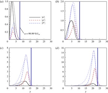
As stated in § 1, the mode T has the largest growth rate in hypersonic cases except for very large $\mathit{Re}$ numbers. Figure 4 shows the modal profiles $|u^{\prime }|~|{\it\rho}^{\prime }|$ and $|T^{\prime }|$ for case M1, M2, M3 and M4 at $\mathit{Re}=400$ and 1000. The disturbance components $v^{\prime }$ and $w^{\prime }$ (not shown in the figure) have much smaller amplitudes. Nevertheless, they take the leading roles in the lift-up mechanism. The boundary layer edge defined as $99.99\,\%~U_{\infty }$ is also plotted in the figure. The four cases have the same wavenumber, B2, but the $\mathit{Ma}$ numbers are different. The disturbances are scaled so that the streamwise velocity disturbance $|u^{\prime }|$ has unit maximum value. With the increase in the $\mathit{Ma}$ number, amplitudes of the disturbance components $|{\it\rho}^{\prime }|$ and $|T^{\prime }|$ become larger. The dominant component, therefore, is the temperature disturbance when $\mathit{Ma}\geqslant 3$ . In moderate supersonic cases ( $\mathit{Ma}=1.5$ , 3.0), the profiles of the disturbances attach to the boundary layer wall while for hypersonic cases ( $\mathit{Ma}=4.5$ , 6.0), all disturbance components detach from the wall. It is evident that the disturbances for $\mathit{Ma}=1.5$ and $\mathit{Ma}=3.0$ belong to the mode W while mode T governs the disturbances for $\mathit{Ma}=4.5$ and $\mathit{Ma}=6.0$ cases. The disturbances of the mode T and mode W are located within the boundary layer. The two types of Görtler mode both are steady and have zero streamwise wavenumber, i.e. ${\it\alpha}_{r}=0$ . The differences between the two modes are reflected in the Reynolds number effect also. By increasing the Reynolds number, the modal shapes tend to become more mature. As a result, the disturbances of the mode W move towards the wall while those for mode T move in the reverse direction when the profiles at $\mathit{Re}=400$ and $\mathit{Re}=1000$ are compared. It should be stressed that the crossover of the two modes (Dando & Seddougui Reference Dando and Seddougui1993; Ren & Fu Reference Ren and Fu2014a ) does not occur in the present study as the $\mathit{Re}$ number is not large enough. Therefore, the linear spatial development of Görtler vortices is governed by the most amplified mode, say, the behaviour of a single mode.

Figure 4.

Disturbance profiles of $|u^{\prime }|$ , $|{\it\rho}^{\prime }|$ and $|T^{\prime }|$ at $\mathit{Re}=400$ (thin lines) and $\mathit{Re}=1000$ (thick lines) with the global spanwise wavenumber $B=1.0\times 10^{-3}$ . The $|u^{\prime }|$ -amplitude is normalized to maintain unit maximum value. The vertical lines show the upper edge of the boundary layer defined as 99.99 % of the freestream velocity. (a) $\mathit{Ma}=1.5$ , (b) $\mathit{Ma}=3.0$ , (c) $\mathit{Ma}=4.5$ , (d) $\mathit{Ma}=6.0$ .

3.2. Spatial development of Görtler vortices

With an understanding of the modal growth, the nonlinear development of Görtler vortices for the five groups of Mach numbers and three wavenumbers are performed. The initial disturbance is introduced into the boundary layer at $\mathit{Re}=200$ with disturbance profiles from the normal mode analysis. The marching reaches a saturated status due to the nonlinear effects for incompressible and moderate compressible flows. In hypersonic flow, the saturation state hardly exists. This will be explained later in this section. The position of the starting point selected here causes no difference to the resulting Görtler vortices (see the discussions by Lee & Liu Reference Lee and Liu1992; Girgis & Liu Reference Girgis and Liu2006). 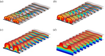The initial amplitude of the disturbances (based on the streamwise velocity disturbance) are specified as $A(u)=2\times 10^{-3}$ to allow sufficient linear growth (see (3.1)). The development of Görtler vortices with spanwise wavenumber B2 in the nonlinear regime for cases M1, M2, M3 and M4 are provided in figure 5. The contours of the streamwise velocity $u$ are at the levels of $0.1,0.2,\ldots ,0.9$ . Ten slices distributed within $\mathit{Re}\in [520,720]$ are plotted to illustrate the rise and development of the mushrooms. The disturbances begin to alter the profiles of the boundary layer visibly at $\mathit{Re}\approx 520$ , where the amplitude of the disturbances reaches 5 % of the base flow. The contours of the density and the temperature are analogous to the streamwise velocity in figure 5.

Figure 5.

Nonlinear development of Görtler vortices and the formation of low- and high-speed streaks. Contour plots of the streamwise velocity are within $\mathit{Re}\in [520,720]$ . Contour $\text{levels}=0.1,0.2,\ldots ,0.9$ . Global spanwise wavenumber $\text{B}2=1.0~\times ~10^{-3}$ . (a) $\mathit{Ma}=1.5$ , (b) $\mathit{Ma}=3.0$ , (c) $\mathit{Ma}=4.5$ , (d) $\mathit{Ma}=6.0$ .

It is seen in figure 5 that the counter-rotating streamwise vortices carry the fluids with high momentum and low temperature towards the wall and fluids with low momentum and high temperature to the reverse direction exerting the lift up mechanism. The boundary layer streaks, and also the thermal streaks (Ricco & Wu Reference Ricco and Wu2007), form as a result. One can observe the changes in the boundary layer due to the increase in the $\mathit{Ma}$ number:

(i) The boundary layer thickness varies with $\mathit{Ma}$ parabolically as ${\it\delta}_{99}\propto \mathit{Ma}^{2}$ . This can be identified from the first slice of the contours in each panel in figure 5 where the boundary layer flow starts to receive perceptible increments from the disturbances.
(ii) Due to the reduction of the growth rate of Görtler modes as $\mathit{Ma}$ number increases, the lift up effect weakens, hampering the formation of the mushrooms. Scrutinizing the two hypersonic cases shown in figure 5(c,d), no mushroom is yet matured. Thus, a bell shape best describes this structure in comparison with the conventional mushroom shape. This phenomenon was first reported by Li et al. (Reference Li, Choudhari, Chang, Wu and Greene2010).
(iii) The moderate supersonic ( $\mathit{Ma}=1.5$ and 3.0) and hypersonic ( $\mathit{Ma}=4.5$ and 6.0) cases are governed by the mode W and mode T, respectively. As a result, the near-wall flows remain uninfluenced, especially in the $\mathit{Ma}=6.0$ case. The thickness of the boundary layer is almost unchanged in the interval of the bells for the $\mathit{Ma}=6.0$ case, whereas in the other cases the streamwise vortices take the high-speed flows towards the wall, hence reducing the thickness of the boundary layer. An unperturbed area where the boundary layer is not affected by the disturbances thus forms in hypersonic cases (also sketched in figure 1).

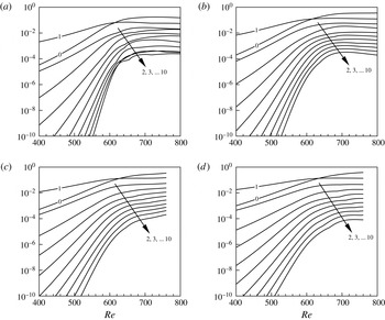
Figure 6 shows the nonlinear development of the amplitude of the Fourier components (based on density disturbances $\hat{{\it\rho}}$ ). The crossover between the base flow correction mode (mode 0) and the fundamental mode (mode 1) occurs in all the cases considered here. The start of the saturation is characterized by the flattening of the disturbance amplitude that clearly occurs for the cases M1 and M2. In the region of saturation, the rapid growth of the amplitudes slows down and is replaced with the redistribution of the disturbance energy among harmonics. In fact, in the non-parallel boundary layer flows which slowly develop in the streamwise direction, a definite saturation may never exist. Comparing the four cases shown in figure 6, the saturation amplitude is not much influenced by the $\mathit{Ma}$ number.

Figure 6.

Development of the amplitude of the disturbances’ Fourier components $\hat{{\it\rho}}_{0}$ , $\hat{{\it\rho}}_{1},\ldots ,\hat{{\it\rho}}_{10}$ as a function of the $\mathit{Re}$ number. The number labelled indicates the wavenumber $n$ of the harmonics as defined in (2.2). (a) $\mathit{Ma}=1.5$ , (b) $\mathit{Ma}=3.0$ , (c) $\mathit{Ma}=4.5$ , (d) $\mathit{Ma}=6.0$ .

Following the definition introduced by Andersson et al. (Reference Andersson, Brandt, Bottaro and Henningson2001), the streak amplitude based on the streamwise velocity disturbance is

(3.1)

$$\begin{eqnarray}A(u)=0.5\left(\max _{y,z}(\tilde{u} )-\min _{y,z}(\tilde{u} )\right).\end{eqnarray}$$

For compressible flows, we also introduce the thermal streak amplitude

(3.2)

$$\begin{eqnarray}A(T)=0.5\left(\max _{y,z}(\tilde{T})-\min _{y,z}(\tilde{T})\right),\end{eqnarray}$$

as a measure of the gradient. The amplitude of the gradient is defined as (see Bottaro & Klingmann Reference Bottaro and Klingmann1996)

(3.3)

$$\begin{eqnarray}\left.\begin{array}{@{}l@{}}A(u_{y})=\displaystyle \max _{y,z}|(U+\tilde{u} )_{y}|,\quad A(u_{z})=\displaystyle \max _{y,z}|(U+\tilde{u} )_{z}|\\ A(T_{y})=\displaystyle \max _{y,z}|(T+\tilde{T})_{y}|,\quad A(T_{z})=\displaystyle \max _{y,z}|(T+\tilde{T})_{z}|.\end{array}\right\}\end{eqnarray}$$

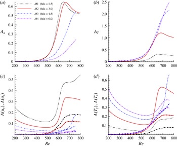
In figure 7(a,b), the streak amplitude $A(u)$ and $A(T)$ are plotted as functions of $\mathit{Re}$ . The global wavenumber $\text{B}2=1.0\times 10^{-3}$ . For the two moderate supersonic cases M1 and M2, $A(u)$ increase first and both reach a maximum value around 0.64. The amplitudes $A(u)$ and $A(T)$ start to decrease in the region of saturation. For the two hypersonic cases M3 and M4, $A(u)$ keeps increasing to 0.54 and 0.24, respectively. A general trend is that the amplitude $A(u)$ decreases while $A(T)$ increases when the Mach number is increased. It is worth noting that $A(T)$ finally reaches 2.2 and 2.5 in M3 and M4 which becomes more than twice that of the base flow. As a result, the nonlinear terms become large enough to require an increasing number of iterations at each station. This creates obstacles for the governing parabolic stability equations and also for the steady development of Görtler vortices in high-speed flows. This is the reason why nonlinear marching becomes difficult to maintain and saturation hardly exists in hypersonic cases. One can improve the situation by increasing the number of harmonics included and reducing the step size ${\rm\Delta}x$ thus diminishing the differences between two steps. The marching is stopped when the mushrooms or bells (based on $A(u)$ and $A(T)$ ) are fully or over developed.

Figure 7.

Spatial development of the streaks indicated with streak amplitude and gradient amplitude. $\mathit{Re}\in [200,800]$ ; $\text{B}2=1.0\times 10^{-3}$ ; $\mathit{Ma}=1.5$ , 3.0, 4.5 and 6.0. (a) Streak amplitude $A(u)$ based on streamwise velocity disturbance $\tilde{u}$ . (b) Streak amplitude $A(T)$ based on temperature disturbance $\tilde{T}$ . (c) Streamwise velocity gradient amplitude $A(u_{y})$ (lines without symbols) and $A(u_{z})$ (with solid circle symbols). (d) Temperature gradient amplitude $A(T_{y})$ (lines without symbols) and $A(T_{z})$ (with solid circle symbols).

Figure 7(c,d) show the amplitude of the gradients for $u_{y}$ , $u_{z}$ and $T_{y}$ , $T_{z}$ defined in (3.3). The lines with and without circle symbols indicate the $y$ - and $z$ -gradient respectively. The $y$ -gradient naturally exists in the undisturbed boundary and thus is not zero when the initial disturbance is introduced. Along with the development of the streak, both $A(u_{y})$ and $A(T_{y})$ first decrease and then increase. In the cases M1 and M2, the saturation finally prevents the rapid growth of this gradient. The $z$ -gradients are generally related to the sinuous secondary mode. In all the cases considered here, they keep growing until the saturation (if it exists) occurs.

On the whole, the $\mathit{Ma}$ number greatly affects the spatial development of Görtler vortices. In addition to the preceding analysis, the increase in the Mach number also brings the following changes to the primary steady states: (i) the temperature disturbance as well as the related gradients become the dominant components; and (ii) saturation of the disturbance hardly exists in hypersonic cases due to the dramatic increase of the temperature disturbances. It can be expected that the secondary instability shall experience a very different scenario depending on the $\mathit{Ma}$ number of the flow.

4. The secondary instability

4.1. Sinuous and varicose modes

The streamwise elongated streaks are receptive to the secondary disturbances when the amplitude is large enough and the secondary instability reaches the maximum growth rate near the saturation of the primary disturbances. To better understand the development of the secondary disturbances, a secondary instability analysis is performed for the fundamental, subharmonic and detuned cases at multiple locations. In this subsection, the secondary perturbations are considered at $\mathit{Re}=700$ .

The secondary instabilities which give rise to the high-frequency unsteady disturbances are regarded as the elementary factor leading to the flow transition. Due to the periodicity of Görtler vortices in the spanwise direction, the secondary instability modes can be divided into odd and even modes which determine the symmetry or antisymmetry of the disturbances. For example, for the odd modes, the secondary disturbances $\tilde{{\it\rho}}_{s}$ , $\tilde{u} _{s}$ , $\tilde{v}_{s}$ and $\tilde{T}_{s}$ are antisymmetric while $\tilde{w}_{s}$ is symmetric in the $y{-}z$ cross section. The even modes have inverse symmetry as do the odd modes. The odd and even modes are essentially responsible for the sinuous and varicose motions of the transition process. Therefore, in this study, they are termed the sinuous and varicose modes respectively.

Figure 8.

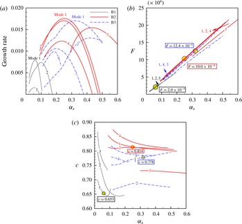
(a) Growth rate of the fundamental secondary disturbances as a function of the streamwise wavenumber ${\it\alpha}_{s}$ at $\mathit{Re}=700$ . Case M1-F-B1, M1-F-B2 and M1-F-B3 are shown. $\mathit{Ma}=1.5$ , ${\it\gamma}_{i}=0$ , $B=0.5,1.0$ and $2.0\times 10^{-3}$ . The labels ‘Mode $1,2,\ldots$ ’ indicate the ranking of maximum growth rate. The most amplified four modes (if they exist) are provided. (b) Dimensionless frequency $F$ (see (2.7)). The dominant frequencies $F=2.0$ , 10.0 and $12.4\times 10^{-4}$ (belong to the largest growth rates) are circled for the three cases. (c) Phase velocity $c$ of the corresponding disturbances. The dominant phase velocity $c=0.653$ , 0.778 and 0.814 are circled.

Generally speaking, a series of varicose and sinuous modes are supported by the fully developed Görtler flows. These modes become amplified within a limited range of wavenumbers or frequencies. Figure 8(a) shows the most amplified four modes (if they exist) for the cases M1-F-B1, M1-F-B2 and M1-F-B3 at $\mathit{Re}=700$ . These secondary modes are labelled ‘mode 1, mode $2\ldots$ ’ according to their maximum growth rates. As shown in the figure, there is an optimal wavenumber ${\it\alpha}_{s,opt}$ for each of the secondary modes. The growth rate decreases when the wavenumber deviates from this value. For the case B1, the growing disturbances occur in a narrower band of the streamwise wavenumbers, i.e. ${\it\alpha}_{s}\in (0,0.2)$ compared to B2 and B3 in which ${\it\alpha}_{s}\in (0,0.6)$ . By examining the peak growth rates of the three cases, the B2 case has the maximum growth rate followed by B3 and B1. Recalling the primary instability shown in figure 3(a), the primary instability observes the same rank as $\text{B}2>\text{B}3>\text{B}1$ . These results show that a larger integrated primary growth, and thus a higher amplitude level, produces the corresponding priority for the secondary instability thus leading to an earlier flow transition. It shall be noticed that some of the modes reach their peak growth rate at an obviously larger wavenumber ${\it\alpha}_{s,opt}$ , e.g. mode 3 for case B2 and mode 2 for case B3. In fact, they are of the sinuous type but have the disturbances concentrated in the stem of the mushroom, which will be highlighted in this study. To distinguish them, they are termed the sinuous mode type II here while the convectional sinuous modes are referred to as sinuous mode type I.

The frequency, to some extent, distinguishes the disturbance types. The dimensionless frequency $F$ of the T–S mode and the Mack second mode (Mack Reference Mack1975, Reference Mack1984), or the mode F/S in the framework suggested by Federov & Tumin (Reference Federov and Tumin2011), has a typical value of $O(10^{-4})$ (see, for example, Ma & Zhong Reference Ma and Zhong2003). Figure 8(b) shows the frequencies of the current secondary disturbances. They are virtually of the order of $O(10^{-3})$ and often termed high-frequency. The varicose and sinuous mode type I with the same spanwise wavenumber $B$ (mode 1, 2, 3 for case B1; mode 1, 2, 4 for B2 and mode 1, 3, 4 for B3) have a very similar frequency while it is smaller for the sinuous mode type II (mode 3 for B2 and mode 2 for B3). The most dangerous frequencies (belonging to the largest growth rate) are $F=2.0$ , 10.0 and $12.4\times 10^{-4}$ for the three cases. As shown in figure 8(b), the frequencies increase almost linearly with the wavenumber ${\it\alpha}_{s}$ showing the phase velocities weakly dependent on the wavenumber (see figure 8 c). The critical phase velocity at the maximum growth rate reads $c=0.653$ , 0.778 and 0.814, respectively for the three cases. The sinuous mode type II has an obviously lower phase velocity.

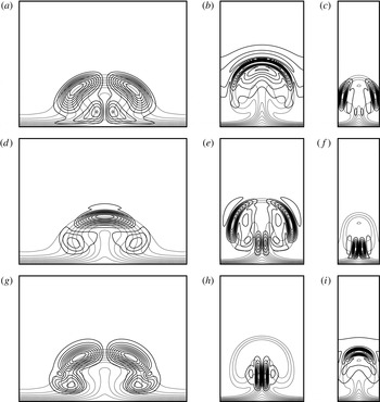
The contours of the streamwise velocity disturbances (absolute value, solid lines) together with the base flow (dashed lines) are plotted in figure 9 at the wavenumber ${\it\alpha}_{s,opt}$ with which they experience the peak growth rates. The most amplified three modes are provided. Both the base flow and the disturbances are normalized to have unit maximum values. The most dangerous mode (mode 1 as indicated in figure 8) for the three wavelengths B1, B2 and B3 are sinuous type I, varicose and sinuous type I, respectively.

Figure 9.

Fundamental secondary disturbances of the most amplified three modes for case M1-F-B1 (a,d,g), M1-F-B2 (b,e,h) and M1-F-B3 (c,f,i) at $\mathit{Re}=700$ ((a,c,e,g) sinuous type I, ( f) sinuous type II, (b,d,i) varicose). Contours of the streamwise velocity disturbance $|\hat{u} _{s}(y,z)|$ (solid lines) and the base flows (dashed lines). Contour $\text{levels}=0.1,0.2,\ldots ,0.9$ . Disturbances subject to the wavenumbers ${\it\alpha}_{s}$ which are the optimal values of ${\it\alpha}_{s,opt}$ at peak growth rates as labelled in each panel. ‘Mode 1, Mode 2 and Mode 3’ correspond to the ranking shown in figure 8. (a) ${\it\alpha}^{s}=0.06$ , (b) ${\it\alpha}^{s}=0.25$ , (c) ${\it\alpha}^{s}=0.32$ , (d) ${\it\alpha}^{s}=0.10$ , (e) ${\it\alpha}^{s}=0.25$ , ( f) ${\it\alpha}^{s}=0.42$ , (g) ${\it\alpha}^{s}=0.06$ , (h) ${\it\alpha}^{s}=0.43$ , (i) ${\it\alpha}^{s}=0.20$ .

4.2. Mach number and wavenumber effects

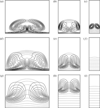
At the same location at $\mathit{Re}=700$ , when the $\mathit{Ma}$ number is increased, the most dangerous modes are all sinuous modes, as can be inferred from figure 10 showing the most dangerous modes for cases M2, M3 and M4. The streamwise wavenumber corresponds to the optimal value ${\it\alpha}_{s,opt}$ of each case. Scrutinizing cases M2-F-B1, M3-F-B1 and M4-F-B1, the $\mathit{Ma}$ number effect is manifested by the secondary disturbances: (i) as discussed in the previous section, the transformation from mode W to mode T uplifts the streaks leaving the near-wall region unperturbed. In other words, the near-wall boundary layer flow is not much affected by Görtler vortices in hypersonic flows. The spanwise shear in the base flow, therefore, concentrates near the upper part of the boundary layer. The sinuous disturbances, consequently, shift towards the upper edge of the boundary layer as the $\mathit{Ma}$ number increases; and (ii) there are three peak values $\hat{u} _{s}$ for case M2-F-B1 but two for M3-F-B1 and one for M4-F-B1. This is due to the reduction in the growth rate of the primary instability which leads to the retrogress of the mushroom. The distortion of the base flow is thus weakened. Furthermore, in M3-F-B3 and M4-F-B3, there are no unstable modes as the streak is too weak.

Figure 10.

Secondary disturbances of the most amplified modes for case M2 (a–c), M3 (d–f) and M4 (g–i) with wavenumbers B1 (a,d,g), B2 (b,e,h) and B3 (c,f,i) at $\mathit{Re}=700$ . Contours of the streamwise velocity disturbance $|\hat{u} _{s}(y,z)|$ (solid lines) and the base flow (dashed lines). Contour $\text{levels}=0.1,0.2,\ldots ,0.9$ . Disturbances subject to wavenumbers ${\it\alpha}_{s}$ which are the optimal values ${\it\alpha}_{s,opt}$ at peak growth rates.

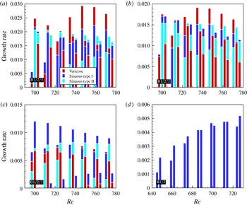
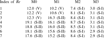
The above analysis is based on a single location corresponding to $\mathit{Re}=700$ . To highlight the effect of Mach number $\mathit{Ma}$ and wavenumber $B$ , results of multiple streamwise locations are summarized in figure 11. Here, the growth rates at seven streamwise locations in the (quasi-) saturated regime are given for cases M0, M1, M2 and M3. The three most dangerous modes, i.e. the varicose mode, sinuous mode type I and sinuous mode type II appear in M0, M1 and M2. In case M3, only the sinuous mode type I exists.

Figure 11.

Growth rates of the secondary disturbances for incompressible, moderate supersonic and hypersonic cases. (a) M0, (b) M1, (c) M2 and (d) M3. Seven streamwise coordinates with $\mathit{Re}=700$ , 713, 726, 738, 750, 762 and 773 are specified for cases M0, M1 and M2 while $\mathit{Re}=647$ , 660, 674, 687, 700, 713 and 725 for case M3. The growth rate is given by the upper bound of the bar with a certain colour. The red, dark blue and light blue bars denote the varicose mode, sinuous mode type I and sinuous mode type II respectively (see also the legend). In the case M3, only the sinuous mode type I exists. Three groups of wavenumbers B1, B2 and B3 (for case M3 only B1 and B2) are shown next to each other as labelled in the left bottom of each panel.

Although high-speed flows are of main interest here, discussions are first given for case M0. Recalling the incompressible study by Li & Malik (Reference Li and Malik1995), these authors showed that the even mode dominated for large wavelengths while the odd mode was more severe for small wavelengths. This conclusion results from the stability analysis up to $x=1.0~\text{m}$ . Within this range, the 18 mm (B2) and 36 mm (B1) wavelength cases had larger growth rates with the even mode while the most dangerous mode in the 9 mm (B3) case was the odd mode. In the experiment (the spanwise wavelength ${\approx}18~\text{mm}$ , case B2), both sinuous and varicose motions arose during the transition process (see Swearingen & Blackwelder Reference Swearingen and Blackwelder1987, figure 14). The sinuous mode is more frequently produced. According to the analysis given by Li & Malik (Reference Li and Malik1995), for this B2 case, the varicose mode had a comparable growth rate to the sinuous mode but maintained the maximum growth rate when the Reynolds number was large. In a recent study, Ren & Fu (Reference Ren and Fu2014b ) revisited the B2 case and realized that the sinuous mode type II was missing in their studies. The sinuous mode type II do exist under experimental conditions however its growth rate is less than the most dangerous mode (varicose mode) (see p. 559, figure 5 Ren & Fu Reference Ren and Fu2014b ). The growth rate of the sinuous mode type II exceeds the varicose mode downstream ( $x>120~\text{cm}$ ) which falls outside the scope of the experimental measurement. In the experimental observation, most of the streaks start to breakdown at around $x=100{-}120~\text{cm}$ burying the sinuous mode type II. It will be elucidated here that this mode can have the largest growth rate downstream and may be responsible for the sinuous transition. For case M0-F-B2, the varicose mode has a larger growth rate than the sinuous mode type I but eventually loses out to the sinuous mode type II from $\mathit{Re}=725$ . It should be emphasized that, besides the growth rate from the Bi-Global stability analysis, receptivity to secondary disturbances (see for example Crouch Reference Crouch1997) and the transient growth (multi-mode behaviour), can influence the outcome of the transition process also. This provides interesting topics for future studies. As a result, it is not common that two adjacent streaks breakdown at the same time. Some of the streaks remain stable as can be found in Swearingen & Blackwelder (Reference Swearingen and Blackwelder1987, pp. 262–263, figures 4 and 5). It can be deduced that the sinuous mode II must have a dominant influence on the streaks which become unstable downstream.

For the other two wavenumbers, case M0-F-B1 is initially dominated by the sinuous mode type I and finally the varicose mode has a considerable advantage. The sinuous mode type II (followed by sinuous mode type I) dominates case M0-F-B3. In short, the conclusion drawn by Li & Malik (Reference Li and Malik1995) reappears in figure 11(a) either if the sinuous mode type II is neglected or the flow condition is limited to the experimental conditions.

In the compressible case with low Mach number, i.e. case M1 in figure 11(b), it is evident that the varicose mode is stronger at small wavenumbers while the sinuous mode takes over at large wavenumbers. This is demonstrated as cases M1-F-B1, M1-F-B2 and M1-F-B3 are governed by the varicose mode, sinuous mode type II and sinuous mode type I, respectively. When the Mach number is increased to 3.0, i.e. case M2 in figure 11(c), the varicose mode loses the competitive edge for the wavenumber B1. Evaluating all three wavenumbers, the overall disturbances fall into the control of the sinuous mode type I. The sinuous mode type I indeed becomes the only existing growing mode in cases M3 (figure 11 d) and M4 (not shown). Figure 11 also illustrates the reduction of the secondary growth rate by increasing the Mach numbers. The stabilizing effect of the Mach number is justified both for the primary and secondary instabilities and hence the flow transition.

The dimensionless frequency $F$ of the dominate disturbance for wavenumber B2 is provided in table 2. Increase in the Mach number reduces this dimensionless frequency. As also shown in figure 8, mode S-II has a considerably larger frequency as this mode achieves its maximum growth rate at a larger wavenumber ${\it\alpha}_{s}$ .

Table 2.

Dimensionless frequency $F$ of the dominant disturbance for wavenumber B2 multiplied by 10⁴. The seven Reynolds number are the same as in figure 11. The type of the secondary mode is given in the brackets.

The sinuous mode type II exists in the incompressible (M0) and the moderately compressible cases (M1 and M2). For the cases evaluated herein, this mode has actually the largest growth rate for the cases M0-F-B2, M0-F-B3 and M1-F-B2 in the saturated regime. Thus, the sinuous mode type II must be closely watched as it can play a very important role in the transition process for subsonic and moderate supersonic flows.

Bottaro & Klingmann (Reference Bottaro and Klingmann1996) formulated a relation between the frequency ${\it\omega}$ or the wavenumber ${\it\alpha}_{s}$ with amplitude $A(U_{z})$ . In the present study, a similar relation is also proposed up to moderate compressible flows for both types of sinuous modes partly reflecting the characteristics of the secondary instability. The scaling with wavenumber B2 is provided below:

(4.1)

$$\begin{eqnarray}{\displaystyle \frac{A(U_{z})}{{\it\omega}_{i}({\it\alpha}_{s,opt})}}=\left\{\begin{array}{@{}ll@{}}0.88\pm 0.06\quad & \text{M0, sinuous mode type I}\\ 0.84\pm 0.04\quad & \text{M1, sinuous mode type I}\\ 0.75\pm 0.06\quad & \text{M2, sinuous mode type I}\\ 0.57\pm 0.03\quad & \text{M0, sinuous mode type II}\\ 0.58\pm 0.02\quad & \text{M1, sinuous mode type II}\\ 0.62\pm 0.03\quad & \text{M2, sinuous mode type II}.\end{array}\right.\end{eqnarray}$$

The values here for the incompressible case are less than 1.2 as given by Bottaro & Klingmann (Reference Bottaro and Klingmann1996). One reason is that different initial amplitudes and different $x$ coordinates are considered. Here, the relationship derived is based on the seven positions at $\mathit{Re}\approx 700$ , 713, 725, 738, 750, 762, 773 (in the saturated regime) where $A(U_{z})$ reaches a quasi-constant state (see figure 7 c). In fact, we find $A(U_{z})/{\it\omega}_{i}({\it\alpha}_{s,opt})$ decreases slowly with $\mathit{Re}$ . Therefore, this ratio must be given together with the parameters ( $\mathit{Re}$ , $\mathit{Ma}$ , initial condition) provided.

In hypersonic cases (M3 and M4), no such a simple relation can be found. Recalling figure 7(c,d), one observes that $A(T_{z})$ becomes the dominant spanwise gradient when $\mathit{Ma}\geqslant 3$ . This is most probably due to the emerging influence of the temperature/density gradients when Mach numbers is increased (see also § 4.3).

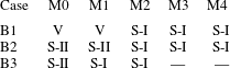
Table 3 summaries the most dangerous modes (with regard to the integrated secondary growth rates in the (quasi-) saturated regime) of the fundamental secondary instabilities for the $\mathit{Ma}$ number and wavenumber investigated. The letter V indicates the varicose mode. S-I and S-II are for the sinuous mode types I and II, respectively. The relationship between the dominant modes (sinuous or varicose) and the spanwise wavenumber put forward by Li & Malik (Reference Li and Malik1995) therefore hold only when the Mach number is not large, even if the sinuous mode type II is ignored. For high-speed flows (in this study $\mathit{Ma}>3$ ), the sinuous mode always has a larger growth rate.

Table 3.

The dominating (fundamental) secondary instability modes. The letter ‘V’, ‘S-I’ and ‘S-II’ indicate the varicose mode, sinuous mode type I and sinuous mode type II.

4.3. Onset conditions

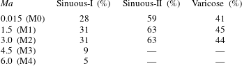
Onset conditions for the five Mach numbers are given in table 4. Results are based on the spanwise wavenumber $B=1\times 10^{-3}$ . The critical streak amplitude $A(u)\approx 28\,\%$ , 59 % and 41 % for the sinuous mode type I, II and the varicose mode, respectively, in the incompressible case (M0). This is close to but larger than the values given by Andersson et al. (Reference Andersson, Brandt, Bottaro and Henningson2001) (26 % and 37 % for sinuous and varicose modes respectively). The reason for this inconsistency could be the following: (i) the primary state of the streak is not exactly the same. The Görtler mode and the Klebanoff mode, though similar, never possess an identical profile. Initial conditions are also not the same. Differences accumulate and feature the spatial development of the streaks; and (ii) though $A(u)$ is a commendable measure of the streak amplitude, it does not tell the whole story through which the shape of the streak is hidden.

Table 4.

Onset conditions of the secondary instability modes measured by the streak amplitude $A(u)$ . Spanwise wavenumber $B=1\times 10^{-3}$ .

In the moderate supersonic cases considered (M1, M2), the critical amplitude $A(u)$ is increased compared with the M0 case. Interestingly, the amplitude is almost identical for the M1 and M2 cases showing that it is the kinetic streak that governs the onset condition in moderate supersonic flows. In hypersonic cases however, the critical amplitude is reduced to 9 % and 5 % for M3 and M4, respectively. Recall § 3.2, a primary feature in hypersonic cases is the significant increase in $A(T)$ and decrease in $A(u)$ highlighting the importance of the thermal streak.

4.4. Subharmonic and detuned modes

The subharmonic and the detuned secondary instabilities of Görtler vortices in high-speed flows also require better understanding. To the authors’ knowledge, this topic has not been well investigated. Here, we focus on the effect of the Floquet parameter ${\it\gamma}$ . The streamwise location is fixed at $\mathit{Re}=700$ .

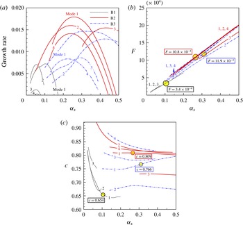
Considering the subharmonic type with ${\it\gamma}_{i}/{\it\beta}=0.5$ , the perturbations experience a $180^{\circ }$ phase change between the mushrooms. The growth rate of disturbances for cases M1-S-B1, M1-S-B2 and M1-S-B3 are given in figure 12(a) as a function of the streamwise wavenumber ${\it\alpha}_{s}$ . The curves are similar to the fundamental counterparts shown in figure 8(a). The sinuous mode type II appears as mode 3 in M1-S-B2 and mode 2 in M1-S-B3. The growth rate for each of the modes is of the same order of amplitude as its fundamental counterpart. The peak growth rate of the most dangerous mode can be smaller (case M1-S-B3) or larger (case M1-S-B2) compared to the fundamental case. Therefore, the subharmonic secondary instability can have the largest growth rate leading to flow transition. The frequency and phase velocity shown in figure 12(b,c) are quite similar to the fundamental case. The sinuous mode type II again stands out. A slight difference in the most dangerous frequency and velocity is observed in figure 12(b,c).

Figure 12.

(a) Growth rate of the subharmonic secondary disturbances as a function of the streamwise wavenumber ${\it\alpha}_{s}$ at $\mathit{Re}=700$ . Cases M1-S-B1, M1-S-B2 and M1-S-B3 are shown. $\mathit{Ma}=1.5$ , ${\it\gamma}_{i}=0.5$ , $B=0.5,1.0$ and $2.0\times 10^{-3}$ . The labels ‘Mode $1,2,\ldots$ ’ indicate the ranking of maximum growth rate. The most amplified four modes (if they exist) are provided. (b) Dimensionless frequency $F$ (see (2.7)). The dominant frequencies $F=3.4$ , 10.8 and $11.9\times 10^{-4}$ (belonging to the largest growth rates) are circled for the three cases. (c) Phase velocity $c$ of the corresponding disturbances. The dominant phase velocity $c=0.654$ , 0.809 and 0.766 are circled.

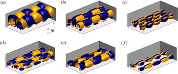
A global view of the normalized disturbance $u_{s}$ (under subharmonic and detuned conditions) of the varicose mode, sinuous mode type I and sinuous mode type II is provided in figure 13. Contour surfaces corresponding to $u_{s}=\pm 0.1$ are coloured blue and yellow, respectively. The plot includes one period in the spanwise and two in the streamwise directions. The disturbance repeats itself in both directions. The detuned mode exhibits a phase change of angle ${\it\psi}$ ( $0^{\circ }<{\it\psi}<180^{\circ }$ , depending on the Floquet parameter ${\it\gamma}$ ) from neighbouring disturbances. In addition to modifications to the steady state (mushrooms or bells), subharmonic and detuned disturbances result in a disruption of the original spanwise periodicity of the primary state.

Figure 13.

Contour surfaces of the normalized streamwise velocity perturbations $u_{s}$ at $\mathit{Ma}=1.5$ , $\mathit{Re}=700$ . The surfaces coloured yellow and blue indicate $u_{s}=0.1$ and $-0.1$ , respectively. One period in spanwise and two periods in streamwise directions are shown. (a) Subharmonic varicose mode, $B=1.0\times 10^{-3}$ , ${\it\alpha}_{s}=0.266$ ; (b) subharmonic sinuous mode type I, $B=1.0\times 10^{-3}$ , ${\it\alpha}_{s}=0.248$ ; (c) subharmonic sinuous mode type II, $B=1.0\times 10^{-3}$ , ${\it\alpha}_{s}=0.428$ ; (d) detuned varicose mode, $B=2.0\times 10^{-3}$ , ${\it\gamma}_{i}=0.24$ , ${\it\alpha}_{s}=0.320$ ; (e) detuned sinuous mode type I, $B=2.0\times 10^{-3}$ , ${\it\gamma}_{i}=0.24$ , ${\it\alpha}_{s}=0.320$ ; ( f) detuned sinuous mode type II, $B=2.0\times 10^{-3}$ , ${\it\gamma}_{i}=0.24$ , ${\it\alpha}_{s}=0.320$ .

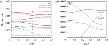
Figure 14(a) shows the growth rate of secondary disturbances as a function of the Floquet parameter ${\it\gamma}$ for M1-D-B1, M1-D-B2 and M1-D-B3. The streamwise wavenumber ${\it\alpha}_{s}$ is specified to the value at which the fundamental disturbance has the maximum growth rate. When ${\it\gamma}_{i}/{\it\beta}$ increases from 0 to 0.5, the growth rate of the mode increases or decreases monotonically. Some modes (e.g. mode 2 in M1-D-B3) are actually insensitive to the Floquet parameter. Detuned modes, therefore, are not dominating in these cases. Computations have been carried out for all the five Mach numbers and three wavenumbers in table 1. We demonstrate that detuned modes generally have smaller growth rates compared with their fundamental or subharmonic counterparts except for case M2-D-B1 ( $\mathit{Ma}=3.0$ ) and M3-D-B1 ( $\mathit{Ma}=4.5$ ). The case M2-D-B1 is highlighted in figure 14(b). Again, the modes are named after their maximum growth rate as mode 1, mode $2\ldots \,$ . The second amplified mode reaches its maximum growth at a detuned state. This phenomenon was not observed in the incompressible case. Within the cases studied in this article, these two exceptions are both the second amplified mode which would not create a primary influence on the transition process.

Figure 14.

Growth rate of the secondary disturbances versus the Floquet parameter ${\it\gamma}$ at $\mathit{Re}=700$ . ‘Mode $1,2\ldots$ ’ are named after the maximum growth rate of the fundamental disturbances (see figure 8 a). (a) Cases M1-D-B1, M1-D-B2 and M1-D-B3. (b) Case M2-D-B1.

In the above analysis, we have shown that Floquet parameter can indeed alter the growth rate of disturbances. This is true for both the streak type flows (Li & Malik Reference Li and Malik1995; Andersson et al. Reference Andersson, Brandt, Bottaro and Henningson2001; Ricco, Luo & Wu Reference Ricco, Luo and Wu2011) and the secondary instability of T–S waves (see Herbert Reference Herbert1988, and the references therein) for which the growth rate of the subharmonic mode can have a distinct difference, larger or smaller than the fundamental type. One notable exception are crossflow vortices. It was shown that the detuned eigensolution can be regarded as a superposition of the eigenfunctions with identical eigenvalues (see Wassermann & Kloker Reference Wassermann and Kloker2005; Bonfigli & Kloker Reference Bonfigli and Kloker2007), thus, having the same growth rate. This is also validated in a recent Floquet analysis (Xu, Liu & Jiang Reference Xu, Liu and Jiang2014).

5. Conclusions

The spatial development and fundamental, subharmonic and detuned secondary instabilities of Görtler vortices in high-speed boundary layer flows are numerically investigated in this paper. Five groups of $\mathit{Ma}$ numbers ( $\mathit{Ma}=0.015$ , $\mathit{Ma}=1.5$ , 3.0, 4.5 and 6.0) are studied to illustrate the compressibility effect. The Görtler vortices with three groups of representative global spanwise wavenumbers ( $B=0.5$ , 1.0 and $2.0\times 10^{-3}$ ) are considered to reveal the effect of primary spanwise wavelength.

The development of Görtler vortices acts to strengthen the boundary layer streaks regardless of the Mach number. In the current study, the streak amplitude $A(u)$ keeps growing downstream (before the right-branch regime is reached). The sinuous mode type I becomes unstable first, followed by the varicose mode and then the sinuous mode type II.

Mach number affects Görtler vortices in two ways: (i) The growth rate of the primary Görtler mode decreases with Mach number. The streaks are thus weakened; and (ii) increase in $\mathit{Ma}$ gives rise to the trapped-layer mode (mode T) for the primary instability. This mode has its disturbances detached from the wall. As a result of the above changes, conventional mushroom structures are replaced by bell-shaped structures, leaving the near-wall region an unperturbed area. The difference in the primary instability leads to a remarkable change on the secondary instability. In subsonic and moderate supersonic flows, varicose and sinuous (type I and type II) modes can both be responsible for the transition process. The sinuous mode type II, whose disturbances concentrate near the stem of the mushroom, is demonstrated to have the largest growth rate when the streak amplitude is large. However, it is missing in existing studies. The relationship between the dominance of sinuous or varicose modes and the primary wavelength in incompressible flow (Li & Malik Reference Li and Malik1995) is no longer valid in hypersonic flows. The sinuous mode becomes the most dangerous regardless of the spanwise wavelength when $\mathit{Ma}>3$ . The effect of the Floquet parameter ${\it\gamma}$ on the growth rate of the secondary instability is clarified. The subharmonic type can become the most dangerous mode, e.g. in the case M2-S-B3. The detuned type, however, is not responsible for the flow transition though in case M2-D-B1 and M3-D-B1, one of the sub-dominant modes reaches its maximum growth rate under detuned state.

The boundary layer transition promoted with concave curvature (Görtler instability), roughness elements or the FST (Klebanoff mode) can follow a similar path utilizing the lift up mechanism. Streamwise curvature acts as an unsophisticated influence, providing a chance to conduct this comprehensive study. The introduction of roughness elements not only brings in discernible wakes which support sinuous and varicose modes, but also creates new mechanisms relating to receptivity, flow separation and shock wave boundary layer interactions. All these phenomena, of course, are closely related to the geometry of the roughness elements. In moderate supersonic flows (Choudhari et al. Reference Choudhari, Li, Chang, Edwards, Kegerise and King2010; De Tullio et al. Reference De Tullio, Paredes, Sandham and Theofilis2013), the varicose mode is demonstrated to be the most dangerous in the wake of diamond ( $\mathit{Ma}=3.5$ ) and square ( $\mathit{Ma}=2.5$ ) shaped roughness elements. In a subsequent study by Choudhari et al. (Reference Choudhari, Li, Chang, Norris and Edwards2013), the Mach number is increased to 5.9 and sinuous perturbations become dominant. In the study of Groskopf, Kloker & Marxen (Reference Groskopf, Kloker, Marxen, Schlatter and Henningson2010) and Kegerise et al. (Reference Kegerise, King, Owens, Choudhari, Norris, Li and Chang2012), the Mach numbers are 4.8 and 3.5, respectively, both types of perturbations emerge. In brief, the various parameters, $\mathit{Re}$ , $\mathit{Ma}$ , shape, height and arrangement of the roughness elements, on the roughness induced transition are far from fully clear. The role of sinuous mode type II in this flow also needs clarification. Future studies are thus required on this topic.

Recalling the discussions in § 3, with an initial amplitude of $A(u)=2\times 10^{-3}$ which is in the range of those observed in the environment, it takes a long distance for the streaks to be matured and for the secondary instabilities to set in (see figure 6). Increase in the $\mathit{Ma}$ number hampers the development of the streaks further and thus may cause failure in flow transition. In some practical situations, for example, before the entrance of the scramjet combustor, this flow behaviour is undesirable. An open question remains as how to achieve optimal control of hypersonic flow transition based on the secondary instability of Görtler vortices.

Acknowledgements

The authors acknowledge financial support from National Natural Science Foundation of China through grants 11272183 and 11572176 and National Key Basic Research Program of China with grant no. 2014CB744801. We would like to thank Professor A. Hanifi for helpful discussions. The anonymous referees provided very valuable comments and suggestions.

Appendix A

The expressions for the operators in (2.3) are given below.

(A 1)

$$\begin{eqnarray}\displaystyle \left.\begin{array}{@{}l@{}}\displaystyle \mathbf{\mathscr{L}}_{0}(1,1)=\frac{1}{h_{1}}\frac{\partial u}{\partial x}+\frac{\partial v}{\partial y}+k\frac{v}{h_{1}}-\text{i}m{\it\omega}\\ \displaystyle \mathbf{\mathscr{L}}_{0}(1,2)=\frac{1}{h_{1}}\frac{\partial {\it\rho}}{\partial x}\\ \mathbf{\mathscr{L}}_{0}(1,3)=\displaystyle \frac{\partial {\it\rho}}{\partial y}+k\frac{{\it\rho}}{h_{1}}\\ \mathbf{\mathscr{L}}_{0}(1,4)=\text{i}n{\it\beta}{\it\rho}\\ \mathbf{\mathscr{L}}_{0}(1,5)=0\end{array}\right\} & & \displaystyle\end{eqnarray}$$

(A 2)

$$\begin{eqnarray}\displaystyle \left.\begin{array}{@{}rcl@{}}\mathbf{\mathscr{L}}_{0}(2,1)\ & =\ & \displaystyle \frac{u}{h_{1}}\frac{\partial u}{\partial x}+v\frac{\partial u}{\partial y}+k\frac{uv}{h_{1}}+\frac{1}{{\it\gamma}\mathit{Ma}^{2}}\frac{1}{h_{1}}\frac{\partial T}{\partial x}\\ \mathbf{\mathscr{L}}_{0}(2,2)\ & =\ & \displaystyle \frac{{\it\rho}}{h_{1}}\frac{\partial u}{\partial x}+k\frac{{\it\rho}v}{h_{1}}+\frac{k}{h_{1}}\frac{\text{d}{\it\mu}}{\text{d}T}\frac{\partial T}{\partial y}\frac{1}{\mathit{Re}_{0}}+27\frac{k^{2}}{h_{1}^{2}}\frac{{\it\mu}}{\mathit{Re}_{0}}-\text{i}m{\it\omega}{\it\rho}-n^{2}{\it\beta}^{2}\frac{{\it\mu}}{\mathit{Re}_{0}}\\ \mathbf{\mathscr{L}}_{0}(2,3)\ & =\ & \displaystyle {\it\rho}\frac{\partial u}{\partial y}+k\frac{{\it\rho}u}{h_{1}}-\frac{4}{3}\frac{k}{h_{1}^{2}}\frac{\text{d}{\it\mu}}{\text{d}T}\frac{\partial T}{\partial x}\frac{1}{\mathit{Re}_{0}}\\ \mathbf{\mathscr{L}}_{0}(2,4)\ & =\ & \displaystyle (\text{i}n{\it\beta})\frac{2}{3}\frac{1}{h_{1}}\frac{\text{d}{\it\mu}}{\text{d}T}\frac{\partial T}{\partial x}\frac{1}{\mathit{Re}_{0}}\\ \mathbf{\mathscr{L}}_{0}(2,5)\ & =\ & \displaystyle -\frac{1}{h_{1}}\frac{\text{d}^{2}{\it\mu}}{\text{d}T^{2}}\frac{\partial T}{\partial x}\frac{1}{\mathit{Re}_{0}}\left(\frac{4}{3}\frac{1}{h_{1}}\frac{\partial u}{\partial x}+\frac{4}{3}\frac{v}{h_{1}}k-\frac{2}{3}\frac{\partial v}{\partial y}\right)\\ \ & \ & \displaystyle -\,\frac{1}{h_{1}}\frac{\text{d}^{2}{\it\mu}}{\text{d}T^{2}}\frac{\partial T}{\partial y}\frac{1}{\mathit{Re}_{0}}\left(h_{1}\frac{\partial u}{\partial y}+\frac{\partial v}{\partial x}-uk\right)\\ \ & \ & \displaystyle -\,\frac{\text{d}{\it\mu}}{\text{d}T}\frac{1}{\mathit{Re}_{0}}\frac{k}{h_{1}}\!\left(\frac{\partial u}{\partial y}+\frac{1}{h_{1}}\frac{\partial v}{\partial x}-k\frac{u}{h_{1}}\right)\!-\frac{1}{h_{1}}\frac{\text{d}{\it\mu}}{\text{d}T}\frac{1}{\mathit{Re}_{0}}\!\left(h_{1}\frac{\partial ^{2}u}{\partial y^{2}}+\frac{\partial ^{2}v}{\partial x\partial y}\right)\\ \ & \ & \displaystyle +\,\frac{1}{{\it\gamma}\mathit{Ma}^{2}}\frac{1}{h_{1}}\frac{\partial {\it\rho}}{\partial x}-\frac{1}{h_{1}}\frac{\text{d}{\it\mu}}{\text{d}T}\frac{1}{\mathit{Re}_{0}}\left(\frac{4}{3}\frac{1}{h_{1}}\frac{\partial ^{2}u}{\partial x^{2}}+\frac{4}{3}\frac{\partial v}{\partial x}\frac{k}{h_{1}}-\frac{2}{3}\frac{\partial ^{2}v}{\partial x\partial y}\right)\end{array}\right\} & & \displaystyle\end{eqnarray}$$

(A 3)

$$\begin{eqnarray}\displaystyle \left.\begin{array}{@{}rcl@{}}\mathbf{\mathscr{L}}_{0}(3,1)\ & =\ & \displaystyle \frac{u}{h_{1}}\frac{\partial v}{\partial x}+v\frac{\partial v}{\partial y}-k\frac{uu}{h_{1}}+\frac{1}{{\it\gamma}\mathit{Ma}^{2}}\frac{\partial T}{\partial y}\\ \mathbf{\mathscr{L}}_{0}(3,2)\ & =\ & \displaystyle \frac{{\it\rho}}{h_{1}}\frac{\partial v}{\partial x}-2k{\it\rho}\frac{u}{h_{1}}+\frac{k}{{h_{1}}^{2}}\frac{1}{\mathit{Re}_{0}}\frac{\text{d}{\it\mu}}{\text{d}T}\frac{\partial T}{\partial x}\\ \mathbf{\mathscr{L}}_{0}(3,3)\ & =\ & \displaystyle {\it\rho}\frac{\partial v}{\partial y}+\frac{2k^{2}}{{h_{1}}^{2}}\frac{{\it\mu}}{\mathit{Re}_{0}}+\frac{2}{3}\frac{1}{\mathit{Re}_{0}}\frac{\text{d}{\it\mu}}{\text{d}T}\frac{\partial T}{\partial y}\frac{k}{h_{1}}-\frac{2}{3}\frac{1}{\mathit{Re}_{0}}{\it\mu}\frac{k^{2}}{h_{1}^{2}}\\ \ & \ & \displaystyle -\,\text{i}m{\it\omega}{\it\rho}-n^{2}{\it\beta}^{2}\frac{{\it\mu}}{\mathit{Re}_{0}}\\ \mathbf{\mathscr{L}}_{0}(3,4)\ & =\ & \displaystyle (\text{i}n{\it\beta})\frac{2}{3}\frac{1}{\mathit{Re}_{0}}\frac{\text{d}{\it\mu}}{\text{d}T}\frac{\partial T}{\partial y}\\ \mathbf{\mathscr{L}}_{0}(3,5)\ & =\ & \displaystyle \frac{1}{{\it\gamma}\mathit{Ma}^{2}}\frac{\partial {\it\rho}}{\partial y}-\frac{1}{h_{1}}\frac{1}{\mathit{Re}_{0}}\frac{\text{d}^{2}{\it\mu}}{\text{d}T^{2}}\frac{\partial T}{\partial x}\left(\frac{\partial u}{\partial y}+\frac{1}{h_{1}}\frac{\partial v}{\partial x}-k\frac{u}{h_{1}}\right)\\ \ & \ & \displaystyle -\,\frac{1}{h_{1}}\frac{1}{\mathit{Re}_{0}}\frac{\text{d}{\it\mu}}{\text{d}T}\left(\frac{\partial ^{2}u}{\partial x\partial y}+\frac{1}{h_{1}}\frac{\partial ^{2}v}{\partial x^{2}}-\frac{\partial u}{\partial x}\frac{k}{h_{1}}\right)\\ \ & \ & \displaystyle -\,\frac{2k}{h_{1}}\frac{1}{\mathit{Re}_{0}}\frac{\text{d}{\it\mu}}{\text{d}T}\left(\frac{\partial v}{\partial y}-\frac{1}{h_{1}}\frac{\partial u}{\partial x}-k\frac{v}{h_{1}}\right)\\ \ & \ & \displaystyle +\,\frac{1}{\mathit{Re}_{0}}\frac{\text{d}^{2}{\it\mu}}{\text{d}T^{2}}\frac{\partial T}{\partial y}\left(\frac{2}{3}\frac{1}{h_{1}}\frac{\partial u}{\partial x}+\frac{2k}{3}\frac{v}{h_{1}}-\frac{4}{3}\frac{\partial v}{\partial y}\right)\\ \ & \ & \displaystyle -\,\frac{1}{\mathit{Re}_{0}}\frac{\text{d}{\it\mu}}{\text{d}T}\left(-\frac{2}{3}\frac{1}{h_{1}}\frac{\partial ^{2}u}{\partial x\partial y}-\frac{2}{3}\frac{k}{h_{1}}\frac{\partial v}{\partial y}+\frac{4}{3}\frac{\partial ^{2}v}{\partial y^{2}}+\frac{2}{3}\frac{k}{{h_{1}}^{2}}\frac{\partial u}{\partial x}+\frac{2}{3}\frac{k^{2}v}{h_{1}^{2}}\right)\end{array}\right\} & & \displaystyle\end{eqnarray}$$

(A 4)

$$\begin{eqnarray}\displaystyle \left.\begin{array}{@{}l@{}}\displaystyle \mathbf{\mathscr{L}}_{0}(4,1)=\text{i}n{\it\beta}\frac{T}{{\it\gamma}\mathit{Ma}^{2}}\\ \displaystyle \mathbf{\mathscr{L}}_{0}(4,2)=-\text{i}n{\it\beta}\frac{1}{h_{1}}\frac{\text{d}{\it\mu}}{\text{d}T}\frac{\partial T}{\partial x}\frac{1}{\mathit{Re}_{0}}\\ \displaystyle \mathbf{\mathscr{L}}_{0}(4,3)=\text{i}n{\it\beta}\left(-\frac{1}{3}{\it\mu}\frac{1}{\mathit{Re}_{0}}\frac{1}{h_{1}}k-\frac{1}{\mathit{Re}_{0}}\frac{\text{d}{\it\mu}}{\text{d}T}\frac{\partial T}{\partial y}\right)\\ \displaystyle \mathbf{\mathscr{L}}_{0}(4,4)=-\text{i}m{\it\omega}{\it\rho}-(n^{2}{\it\beta}^{2})\frac{3}{4}\frac{{\it\mu}}{\mathit{Re}_{0}}\\ \displaystyle \mathbf{\mathscr{L}}_{0}(4,5)=\text{i}n{\it\beta}\left(\frac{1}{{\it\gamma}\mathit{Ma}^{2}}{\it\rho}-\frac{\partial {\it\mu}}{\partial T}\left(-\frac{2}{3}\frac{1}{\mathit{Re}_{0}}\frac{1}{h_{1}}\frac{\partial u}{\partial x}-\frac{2}{3}\frac{1}{\mathit{Re}_{0}}\frac{vk}{h_{1}}-\frac{2}{3}\frac{1}{\mathit{Re}_{0}}\frac{\partial v}{\partial y}\right)\right)\end{array}\right\} & & \displaystyle\end{eqnarray}$$

(A 5)

$$\begin{eqnarray}\displaystyle \left.\begin{array}{@{}rcl@{}}\mathbf{\mathscr{L}}_{0}(5,1)\ & =\ & \displaystyle \frac{u}{h_{1}}\frac{\partial T}{\partial x}+v\frac{\partial T}{\partial y}-\frac{{\it\gamma}-1}{{\it\gamma}}\frac{u}{h_{1}}\frac{\partial T}{\partial x}-\frac{{\it\gamma}-1}{{\it\gamma}}v\frac{\partial T}{\partial y}+\text{i}m{\it\omega}\frac{{\it\gamma}-1}{{\it\gamma}}T\\ \mathbf{\mathscr{L}}_{0}(5,2)\ & =\ & \displaystyle \frac{{\it\rho}}{h_{1}}\frac{\partial T}{\partial x}-\frac{{\it\gamma}-1}{{\it\gamma}}\left(\frac{1}{h_{1}}{\it\rho}\frac{\partial T}{\partial x}+\frac{1}{h_{1}}T\frac{\partial {\it\rho}}{\partial x}\right)\\ \ & \ & \displaystyle +\,2\frac{({\it\gamma}-1)\mathit{Ma}^{2}}{\mathit{Re}_{0}}{\it\mu}\left(-\frac{k^{2}}{{h_{1}}^{2}}u+\frac{k}{{h_{1}}^{2}}\frac{\partial v}{\partial x}+\frac{\partial u}{\partial y}\frac{k}{h_{1}}\right)\\ \mathbf{\mathscr{L}}_{0}(5,3)\ & =\ & \displaystyle {\it\rho}\frac{\partial T}{\partial y}-\frac{{\it\gamma}-1}{{\it\gamma}}\left({\it\rho}\frac{\partial T}{\partial y}+T\frac{\partial {\it\rho}}{\partial y}\right)\\ \ & \ & \displaystyle -\,2\frac{({\it\gamma}-1)\mathit{Ma}^{2}}{\mathit{Re}_{0}}{\it\mu}\left(\frac{4}{3}\frac{k}{{h_{1}}^{2}}\frac{\partial u}{\partial x}+\frac{4}{3}\frac{k^{2}v}{{h_{1}}^{2}}-\frac{2}{3}\frac{k}{h_{1}}\frac{\partial v}{\partial y}\right)\\ \mathbf{\mathscr{L}}_{0}(5,4)\ & =\ & \displaystyle (\text{i}n{\it\beta})\frac{4}{3}\frac{({\it\gamma}-1)\mathit{Ma}^{2}}{\mathit{Re}_{0}}{\it\mu}\left(\frac{1}{h_{1}}\frac{\partial u}{\partial x}+\frac{vk}{h_{1}}+\frac{\partial v}{\partial y}\right)\\ \mathbf{\mathscr{L}}_{0}(5,5)\ & =\ & \displaystyle -\frac{{\it\gamma}-1}{{\it\gamma}}\frac{u}{h_{1}}\frac{\partial {\it\rho}}{\partial x}-\frac{{\it\gamma}-1}{{\it\gamma}}v\frac{\partial {\it\rho}}{\partial y}-\frac{1}{\mathit{Re}_{0}\mathit{Pr}}\frac{1}{{h_{1}}^{2}}\frac{\text{d}^{2}{\it\kappa}}{\text{d}T^{2}}\frac{\partial T}{\partial x}\frac{\partial T}{\partial x}\\ \ & \ & \displaystyle -\,\frac{1}{\mathit{Re}_{0}\mathit{Pr}}\frac{1}{{h_{1}}^{2}}\frac{\text{d}{\it\kappa}}{\text{d}T}\frac{\partial ^{2}T}{\partial x^{2}}-\frac{1}{\mathit{Re}_{0}\mathit{Pr}}\frac{\text{d}^{2}{\it\kappa}}{\text{d}T^{2}}\frac{\partial T}{\partial y}\frac{\partial T}{\partial y}\\ \ & \ & \displaystyle -\,\frac{1}{\mathit{Re}_{0}\mathit{Pr}}\frac{k}{h_{1}}\frac{\text{d}{\it\kappa}}{\text{d}T}\frac{\partial T}{\partial y}-\frac{1}{\mathit{Re}_{0}\mathit{Pr}}\frac{\text{d}{\it\kappa}}{\text{d}T}\frac{\partial ^{2}T}{\partial y^{2}}\\ \ & \ & \displaystyle -\,\frac{({\it\gamma}-1)\mathit{Ma}^{2}}{\mathit{Re}_{0}}\frac{\text{d}{\it\mu}}{\text{d}T}\left(\frac{4}{3}\left(\frac{1}{h_{1}}\frac{\partial u}{\partial x}+\frac{vk}{h_{1}}\right)^{2}+\frac{4}{3}\frac{\partial v}{\partial y}\frac{\partial v}{\partial y}\right)\\ \ & \ & \displaystyle -\,\frac{({\it\gamma}-1)\mathit{Ma}^{2}}{\mathit{Re}_{0}}\frac{\text{d}{\it\mu}}{\text{d}T}\left(-\frac{4}{3}\left(\frac{1}{h_{1}}\frac{\partial u}{\partial x}+\frac{vk}{h_{1}}\right)\left(\frac{\partial v}{\partial y}\right)\right.\\ \ & \ & \displaystyle \left.+\left(\frac{1}{h_{1}}\frac{\partial v}{\partial x}+\frac{\partial u}{\partial y}-\frac{uk}{h_{1}}\right)^{2}\right)\\ \ & \ & \displaystyle -\,\text{i}m{\it\omega}\left(\frac{{\it\rho}}{{\it\gamma}}\right)-n^{2}{\it\beta}^{2}\frac{{\it\kappa}}{\mathit{Re}_{0}\mathit{Pr}}\end{array}\right\} & & \displaystyle\end{eqnarray}$$

(A 6a−c )

$$\begin{eqnarray}\mathbf{\mathscr{L}}_{1}(1,1)=\frac{u}{h_{1}},\quad \mathbf{\mathscr{L}}_{1}(1,2)=\frac{{\it\rho}}{h_{1}},\quad \mathbf{\mathscr{L}}_{1}(1,3)=\mathbf{\mathscr{L}}_{1}(1,4)=\mathbf{\mathscr{L}}_{1}(1,5)=0\end{eqnarray}$$

(A 7)

$$\begin{eqnarray}\displaystyle \left.\begin{array}{@{}l@{}}\displaystyle \mathbf{\mathscr{L}}_{1}(2,1)=\frac{1}{{\it\gamma}\mathit{Ma}^{2}}\frac{1}{h_{1}}T\\ \displaystyle \mathbf{\mathscr{L}}_{1}(2,2)={\it\rho}\frac{u}{h_{1}}-\frac{1}{{h_{1}}^{2}}\frac{4}{3}\frac{\text{d}{\it\mu}}{\text{d}T}\frac{\partial T}{\partial x}\frac{1}{\mathit{Re}_{0}}\\ \displaystyle \mathbf{\mathscr{L}}_{1}(2,3)=-\frac{4}{3}\frac{k}{{h_{1}}^{2}}\frac{{\it\mu}}{\mathit{Re}_{0}}-\frac{1}{h_{1}}\frac{\text{d}{\it\mu}}{\text{d}T}\frac{\partial T}{\partial y}\frac{1}{\mathit{Re}_{0}}-\frac{k}{{h_{1}}^{2}}\frac{{\it\mu}}{\mathit{Re}_{0}}\\ \displaystyle \mathbf{\mathscr{L}}_{1}(2,4)=-(\text{i}n{\it\beta})\frac{1}{3}\frac{1}{h_{1}}\frac{{\it\mu}}{\mathit{Re}_{0}}\\ \displaystyle \mathbf{\mathscr{L}}_{1}(2,5)=-\frac{1}{h_{1}}\frac{\text{d}{\it\mu}}{\text{d}T}\frac{1}{\mathit{Re}_{0}}\left(\frac{4}{3}\frac{1}{h_{1}}\frac{\partial u}{\partial x}+\frac{4}{3}\frac{vk}{h_{1}}-\frac{2}{3}\frac{\partial v}{\partial y}\right)+\frac{1}{{\it\gamma}\mathit{Ma}^{2}}\frac{{\it\rho}}{h_{1}}\end{array}\right\} & & \displaystyle\end{eqnarray}$$

(A 8)

$$\begin{eqnarray}\displaystyle \left.\begin{array}{@{}l@{}}\mathbf{\mathscr{L}}_{1}(3,1)=0\\ \displaystyle \mathbf{\mathscr{L}}_{1}(3,2)=\frac{3}{{h_{1}}^{2}}k\frac{1}{\mathit{Re}_{0}}{\it\mu}+\frac{2}{3}\frac{1}{\mathit{Re}_{0}}\frac{\text{d}{\it\mu}}{\text{d}T}\frac{\partial T}{\partial y}\frac{1}{h_{1}}-\frac{2}{3}k\frac{{\it\mu}}{\mathit{Re}_{0}}\frac{1}{{h_{1}}^{2}}\\ \displaystyle \mathbf{\mathscr{L}}_{1}(3,3)={\it\rho}\frac{u}{h_{1}}-\frac{1}{{h_{1}}^{2}}\frac{1}{\mathit{Re}_{0}}\frac{\text{d}{\it\mu}}{\text{d}T}\frac{\partial T}{\partial x}\\ \mathbf{\mathscr{L}}_{1}(3,4)=0\\ \displaystyle \mathbf{\mathscr{L}}_{1}(3,5)=-\frac{1}{h_{1}}\frac{1}{\mathit{Re}_{0}}\frac{\text{d}{\it\mu}}{\text{d}T}\left(\frac{\partial u}{\partial y}+\frac{1}{h_{1}}\frac{\partial v}{\partial x}-\frac{u}{h_{1}}k\right)\end{array}\right\} & & \displaystyle\end{eqnarray}$$

(A 9)

$$\begin{eqnarray}\displaystyle \left.\begin{array}{@{}l@{}}\mathbf{\mathscr{L}}_{1}(4,1)=0\\ \displaystyle \mathbf{\mathscr{L}}_{1}(4,2)=-(\text{i}n{\it\beta})\frac{1}{3}\frac{1}{h_{1}}\frac{{\it\mu}}{\mathit{Re}_{0}}\\ \mathbf{\mathscr{L}}_{1}(4,3)=0\\ \displaystyle \mathbf{\mathscr{L}}_{1}(4,4)={\it\rho}\frac{u}{{h_{1}}^{2}}-\frac{1}{h_{1}}\frac{\text{d}{\it\mu}}{\text{d}T}\frac{\partial T}{\partial x}\frac{1}{\mathit{Re}_{0}}\\ \mathbf{\mathscr{L}}_{1}(4,5)=0\end{array}\right\} & & \displaystyle\end{eqnarray}$$

(A 10)

$$\begin{eqnarray}\displaystyle \left.\begin{array}{@{}l@{}}\displaystyle \mathbf{\mathscr{L}}_{1}(5,1)=-\frac{{\it\gamma}-1}{{\it\gamma}}T\frac{u}{h_{1}}\\ \displaystyle \mathbf{\mathscr{L}}_{1}(5,2)=\frac{4}{3}\frac{({\it\gamma}-1)\mathit{Ma}^{2}}{\mathit{Re}_{0}}{\it\mu}\left(\frac{1}{h_{1}}\frac{\partial v}{\partial y}-\frac{2}{{h_{1}}^{2}}\frac{\partial u}{\partial x}-\frac{2vk}{{h_{1}}^{2}}\right)\\ \displaystyle \mathbf{\mathscr{L}}_{1}(5,3)=-2\frac{({\it\gamma}-1)\mathit{Ma}^{2}}{\mathit{Re}_{0}}{\it\mu}\left(\frac{1}{{h_{1}}^{2}}\frac{\partial v}{\partial x}+\frac{1}{h_{1}}\frac{\partial u}{\partial y}-\frac{uk}{{h_{1}}^{2}}\right)\\ \mathbf{\mathscr{L}}_{1}(5,4)=0\\ \displaystyle \mathbf{\mathscr{L}}_{1}(5,5)=\frac{{\it\rho}}{{\it\gamma}}\frac{u}{h_{1}}-\frac{2}{\mathit{Re}_{0}\mathit{Pr}}\frac{1}{{h_{1}}^{2}}\frac{\text{d}{\it\kappa}}{\text{d}T}\frac{\partial T}{\partial x}\end{array}\right\} & & \displaystyle\end{eqnarray}$$

(A 11)

$$\begin{eqnarray}\left.\begin{array}{@{}c@{}}\mathbf{\mathscr{L}}_{2}(1,1)=v\\ \mathbf{\mathscr{L}}_{2}(1,2)=0\\ \mathbf{\mathscr{L}}_{2}(1,3)={\it\rho}\\ \mathbf{\mathscr{L}}_{2}(1,4)=0\\ \mathbf{\mathscr{L}}_{2}(1,5)=0\end{array}\right\}\end{eqnarray}$$

(A 12)

$$\begin{eqnarray}\displaystyle \left.\begin{array}{@{}l@{}}\mathbf{\mathscr{L}}_{2}(2,1)=0\\ \displaystyle \mathbf{\mathscr{L}}_{2}(2,2)={\it\rho}v-\frac{\text{d}{\it\mu}}{\text{d}T}\frac{\partial T}{\partial y}\frac{1}{\mathit{Re}_{0}}-\frac{{\it\mu}}{\mathit{Re }_{0}}\frac{k}{h_{1}}\\ \displaystyle \mathbf{\mathscr{L}}_{2}(2,3)=\frac{2}{3}\frac{\text{d}{\it\mu}}{\text{d}T}\frac{\partial T}{\partial x}\frac{1}{\mathit{Re}_{0}}\frac{1}{h_{1}}\\ \mathbf{\mathscr{L}}_{2}(2,4)=0\\ \displaystyle \mathbf{\mathscr{L}}_{2}(2,5)=-\frac{1}{h_{1}}\frac{\text{d}{\it\mu}}{\text{d}T}\frac{1}{\mathit{Re}_{0}}\left(h_{1}\frac{\partial u}{\partial y}+\frac{\partial v}{\partial x}-uk\right)\end{array}\right\} & & \displaystyle\end{eqnarray}$$

(A 13)

$$\begin{eqnarray}\displaystyle \left.\begin{array}{@{}l@{}}\displaystyle \mathbf{\mathscr{L}}_{2}(3,1)=\frac{T}{{\it\gamma}\mathit{Ma}^{2}}\\ \displaystyle \mathbf{\mathscr{L}}_{2}(3,2)=-\frac{1}{h_{1}}\frac{1}{\mathit{Re}_{0}}\frac{\text{d}{\it\mu}}{\text{d}T}\frac{\partial T}{\partial x}\\ \displaystyle \mathbf{\mathscr{L}}_{2}(3,3)={\it\rho}v-\frac{2k}{h_{1}}\frac{{\it\mu}}{\mathit{Re}_{0}}-\frac{4}{3}\frac{1}{\mathit{Re}_{0}}\frac{\text{d}{\it\mu}}{\text{d}T}\frac{\partial T}{\partial y}+\frac{2}{3}\frac{{\it\mu}}{\mathit{Re}_{0}}\frac{k}{h_{1}}\\ \displaystyle \mathbf{\mathscr{L}}_{2}(3,4)=-\text{i}n{\it\beta}\frac{1}{3}\frac{{\it\mu}}{\mathit{Re}_{0}}\\ \displaystyle \mathbf{\mathscr{L}}_{2}(3,5)=\frac{{\it\rho}}{{\it\gamma}\mathit{Ma }^{2}}+\frac{1}{\mathit{Re}_{0}}\frac{\text{d}{\it\mu}}{\text{d}T}\left(\frac{2}{3}\frac{1}{h_{1}}\frac{\partial u}{\partial x}+\frac{2}{3}\frac{vk}{h_{1}}-\frac{4}{3}\frac{\partial v}{\partial y}\right)\end{array}\right\} & & \displaystyle\end{eqnarray}$$

(A 14)

$$\begin{eqnarray}\displaystyle \left.\begin{array}{@{}l@{}}\mathbf{\mathscr{L}}_{2}(4,1)=0\\ \mathbf{\mathscr{L}}_{2}(4,2)=0\\ \displaystyle \mathbf{\mathscr{L}}_{2}(4,3)=-\text{i}n{\it\beta}\frac{1}{3}\frac{{\it\mu}}{\mathit{Re}_{0}}\\ \displaystyle \mathbf{\mathscr{L}}_{2}(4,4)={\it\rho}v-\frac{k}{h_{1}}\frac{{\it\mu}}{\mathit{Re}_{0}}-\frac{1}{\mathit{Re}_{0}}\frac{\text{d}{\it\mu}}{\text{d}T}\frac{\partial T}{\partial y}\\ \mathbf{\mathscr{L}}_{2}(4,5)=0\end{array}\right\} & & \displaystyle\end{eqnarray}$$

(A 15)

$$\begin{eqnarray}\displaystyle \left.\begin{array}{@{}l@{}}\displaystyle \mathbf{\mathscr{L}}_{2}(5,1)=-\frac{{\it\gamma}-1}{{\it\gamma}}Tv\\ \displaystyle \mathbf{\mathscr{L}}_{2}(5,2)=-2\frac{({\it\gamma}-1)\mathit{Ma}^{2}}{\mathit{Re}_{0}}{\it\mu}\left(\frac{\partial u}{\partial y}+\frac{1}{h_{1}}\frac{\partial v}{\partial x}-\frac{uk}{h_{1}}\right)\\ \displaystyle \mathbf{\mathscr{L}}_{2}(5,3)=\frac{4}{3}\frac{({\it\gamma}-1)\mathit{Ma}^{2}}{\mathit{Re}_{0}}{\it\mu}\left(-2\frac{\partial v}{\partial y}+\frac{1}{h_{1}}\frac{\partial u}{\partial x}+\frac{vk}{h_{1}}\right)\\ \mathbf{\mathscr{L}}_{2}(5,4)=0\\ \displaystyle \mathbf{\mathscr{L}}_{2}(5,5)=\frac{{\it\rho}v}{{\it\gamma}}-\frac{2}{\mathit{Re}_{0}\mathit{Pr}}\frac{\text{d}{\it\kappa}}{\text{d}T}\frac{\partial T}{\partial y}-\frac{1}{\mathit{Re}_{0}\mathit{Pr}}\frac{k}{h_{1}}{\it\kappa}.\end{array}\right\} & & \displaystyle\end{eqnarray}$$

Only non-zero components are given for $\mathbf{\mathscr{L}}_{3}$ , $\mathbf{\mathscr{L}}_{4}$ and $\mathbf{\mathscr{L}}_{5}$

(A 16a−c )

$$\begin{eqnarray}\mathbf{\mathscr{L}}_{3}(2,2)=-\frac{4}{3}\frac{1}{h_{1}^{2}}\frac{{\it\mu}}{\mathit{Re}_{0}},\quad \mathbf{\mathscr{L}}_{3}(3,3)=\mathbf{\mathscr{L}}_{3}(4,4)=-\frac{1}{h_{1}^{2}}\frac{{\it\mu}}{\mathit{Re}_{0}},\quad \mathbf{\mathscr{L}}_{3}(5,5)=-\frac{1}{h_{1}^{2}}\frac{{\it\kappa}}{\mathit{Re}_{0}\mathit{Pr}}\vphantom{\mathop{\sum }_{\sum }}\end{eqnarray}$$

(A 17)

$$\begin{eqnarray}\mathbf{\mathscr{L}}_{4}(2,3)=\mathbf{\mathscr{L}}_{4}(3,2)=-\frac{1}{3}\frac{1}{h_{1}}\frac{{\it\mu}}{\mathit{Re}_{0}}\end{eqnarray}$$

(A 18a−c )

$$\begin{eqnarray}\mathbf{\mathscr{L}}_{5}(2,2)=\mathbf{\mathscr{L}}_{5}(4,4)=-\frac{{\it\mu}}{\mathit{Re}_{0}},\quad \mathbf{\mathscr{L}}_{5}(3,3)=-\frac{4}{3}\frac{{\it\mu}}{\mathit{Re}_{0}},\quad \mathbf{\mathscr{L}}_{5}(5,5)=-\frac{{\it\kappa}}{\mathit{Re}_{0}\mathit{Pr}}.\end{eqnarray}$$

References

Andersson, P., Berggren, M. & Henningson, D. S. 1999 Optimal disturbances and bypass transition in boundary layers. Phys. Fluids 11 (1), 134–150.CrossRef Google Scholar

Andersson, P., Brandt, L., Bottaro, A. & Henningson, D. S. 2001 On the breakdown of boundary layer streaks. J. Fluid Mech. 428, 29–60.CrossRef Google Scholar

Asai, M., Minagawa, M. & Nishioka, M. 2002 The instability and breakdown of a near-wall low-speed streak. J. Fluid Mech. 455, 289–314.CrossRef Google Scholar

Bassom, A. P. & Hall, P. 1994 The receptivity problem for

$O(1)$ wavelength Görtler vortices. Proc. R. Soc. Lond. A 446 (1928), 499–516.Google Scholar

Bassom, A. P. & Seddougui, S. O. 1995 Receptivity mechanisms for Görtler vortex modes. Theor. Comput. Fluid Dyn. 7 (5), 317–339.CrossRef Google Scholar

Bonfigli, G. & Kloker, M. 2007 Secondary instability of crossflow vortices: validation of the stability theory by direct numerical simulation. J. Fluid Mech. 583, 229–272.CrossRef Google Scholar

Bottaro, A. & Klingmann, B. G. B. 1996 On the linear breakdown of Görtler vortices. Eur. J. Mech. (B/Fluids) 15 (3), 301–330.Google Scholar

Bottaro, A. & Luchini, P. 1999 Görtler vortices: Are they amenable to local eigenvalue analysis? Eur. J. Mech. (B/Fluids) 18 (1), 47–65.CrossRef Google Scholar

de la Chevalerie, D. A., Fonteneau, A., Luca, L. D. & Cardone, G. 1997 Görtler-type vortices in hypersonic flows: the ramp problem. Exp. Therm. Fluid Sci. 15 (2), 69–81.CrossRef Google Scholar

Chen, F.-J., Wilkinson, S. P. & Beckwith, I. E. 1993 Görtler instability and hypersonic quiet nozzle design. J. Spacecr. Rockets 30 (2), 170–175.CrossRef Google Scholar

Choudhari, M., Li, F., Chang, C.-L., Edwards, J., Kegerise, M. & King, R.2010 Laminar-turbulent transition behind discrete roughness elements in a high-speed boundary layer. In 48th AIAA Aerospace Sciences Meeting Including the New Horizons Forum and Aerospace Exposition, AIAA-2010-1575. American Institute of Aeronautics and Astronautics (AIAA).CrossRef Google Scholar

Choudhari, M., Li, F., Chang, C.-L., Norris, A. & Edwards, J.2013 Wake instabilities behind discrete roughness elements in high speed boundary layers. In 51st AIAA Aerospace Sciences Meeting including the New Horizons Forum and Aerospace Exposition, AIAA-2013-0081.Google Scholar

Crouch, J. D. 1997 Excitation of secondary instabilities in boundary layers. J. Fluid Mech. 336, 245–266.CrossRef Google Scholar

Dando, A. H. & Seddougui, S. O. 1993 The compressible Görtler problem in two-dimensional boundary layers. IMA J. Appl. Maths 51 (1), 27–67.CrossRef Google Scholar

Day, H. P., Herbert, T. & Saric, W. S. 1990 Comparing local and marching analysis of Görtler instability. AIAA J. 28 (6), 1010–1015.CrossRef Google Scholar

Denier, J. P., Hall, P. & Seddougui, S. O. 1991 On the receptivity problem for Görtler vortices: vortex motions induced by wall roughness. Phil. Trans. R. Soc. Lond. A 335 (1636), 51–85.Google Scholar

De Tullio, N., Paredes, P., Sandham, N. D. & Theofilis, V. 2013 Laminar-turbulent transition induced by a discrete roughness element in a supersonic boundary layer. J. Fluid Mech. 735, 613–646.CrossRef Google Scholar

Dong, M. & Wu, X. 2013 On continuous spectra of the orr-sommerfeld/squire equations and entrainment of free-stream vortical disturbances. J. Fluid Mech. 732, 616–659.CrossRef Google Scholar

Ellingsen, T. & Palm, E. 1975 Stability of linear flow. Phys. Fluids 18 (4), 487–488.CrossRef Google Scholar

Federov, A. & Tumin, A. 2011 High-speed boundary-layer instability: old terminology and a new framework. AIAA J. 49 (8), 1647–1657.CrossRef Google Scholar

Floryan, J. M. 1991 On the Görtler instability of boundary layers. Prog. Aerosp. Sci. 28 (3), 235–271.CrossRef Google Scholar

Fu, Y. & Hall, P. 1992 Nonlinear development and secondary instability of large-amplitude Görtler vortices in hypersonic boundary-layers. Eur. J. Mech. (B/Fluids) 11 (4), 465–510.Google Scholar

Fu, Y. & Hall, P. 1993 Effects of Görtler vortices, wall cooling and gas dissociation on the Rayleigh instability in a hypersonic boundary layer. J. Fluid Mech. 247, 503–525.CrossRef Google Scholar

Girgis, I. G. & Liu, J. T. C. 2006 Nonlinear mechanics of wavy instability of steady longitudinal vortices and its effect on skin friction rise in boundary layer flow. Phys. Fluids 18 (2), 024102.CrossRef Google Scholar

Görtler, H. 1940 Über eine dreidimensionale instabilität laminarer grenzschichten an konkaven wänden. Ges. D. Wiss. Göttingen, Nachr 1 (2), translated as ‘On the three-dimensional instability of laminar boundary layers on concave walls. NACA TM 1375, 1954’.Google Scholar

Goulpié, P., Klingmann, B. G. B. & Bottaro, A. 1996 Görtler vortices in boundary layers with streamwise pressure gradient: linear theory. Phys. Fluids 8 (2), 451–459.CrossRef Google Scholar

Groskopf, G., Kloker, M. J. & Marxen, O. 2010 Bi-global crossplane stability analysis of high-speed boundary-layer flows with discrete roughness. In 7th IUTAM Symposium on Laminar–Turbulent Transition (ed. Schlatter, P. & Henningson, D. S.), IUTAM Bookseries, vol. 18, pp. 171–176. Springer.CrossRef Google Scholar

Hall, P. 1982 Taylor–Gortler vortices in fully developed or boundary-layer flows: linear theory. J. Fluid Mech. 124, 475–494.CrossRef Google Scholar

Hall, P. 1983 The linear development of Görtler vortices in growing boundary layers. J. Fluid Mech. 130, 41–58.CrossRef Google Scholar

Hall, P. 1990 Görtler vortices in growing boundary layers: the leading edge receptivity problem, linear growth and the nonlinear breakdown stage. Mathematika 37, 151–189.CrossRef Google Scholar

Hall, P. & Fu, Y. 1989 On the Görtler vortex instability mechanism at hypersonic speeds. Theor. Comput. Fluid Dyn. 1 (3), 125–134.CrossRef Google Scholar

Hall, P. & Horseman, N. J. 1991 The linear inviscid secondary instability of longitudinal vortex structures in boundary layers. J. Fluid Mech. 232, 357–375.CrossRef Google Scholar

Hanifi, A., Schmid, P. J. & Henningson, D. S. 1996 Transient growth in compressible boundary layer flow. Phys. Fluids 8 (3), 826–837.CrossRef Google Scholar

Herbert, T. 1976 On the stability of the boundary layer along a concave wall. Arch. Mech. Stosowanej 28 (5–6), 1039–1055.Google Scholar

Herbert, T. 1988 Secondary instability of boundary layers. Annu. Rev. Fluid Mech. 20, 487–526.CrossRef Google Scholar

Hultgren, L. S. & Gustavsson, L. H. 1981 Algebraic growth of disturbances in a laminar boundary layer. Phys. Fluids 24 (6), 1000–1004.CrossRef Google Scholar

Joslin, R. D. & Grosch, C. E. 1995 Growth characteristics downstream of a shallow bump: computation and experiment. Phys. Fluids 7 (12), 3042–3047.CrossRef Google Scholar

Kegerise, M. A., King, R. A., Owens, L. R., Choudhari, M. M., Norris, A. T., Li, F. & Chang, C.-L.2012 An experimental and numerical study of roughness-induced instabilities in a Mach 3.5 boundary layer. In RTO AVT-200 RSM-030 Specialists’ Meeting on Hypersonic Laminar–Turbulent Transition, nF1676L-14423.Google Scholar

Landahl, M. T. 1975 Wave breakdown and turbulence. SIAM J. Appl. Maths 28 (4), 735–756.CrossRef Google Scholar

Landahl, M. T. 1980 A note on an algebraic instability of inviscid parallel shear flows. J. Fluid Mech. 98, 243–251.CrossRef Google Scholar

Lee, K. & Liu, J. T. C. 1992 On the growth of mushroomlike structures in nonlinear spatially developing Goertler vortex flow. Phys. Fluids A 4 (1), 95–103.CrossRef Google Scholar

Leib, S. J., Wundrow, D. W. & Goldstein, M. E. 1999 Effect of free-stream turbulence and other vortical disturbances on a laminar boundary layer. J. Fluid Mech. 380, 169–203.CrossRef Google Scholar

Li, F., Choudhari, M., Chang, C.-L., Wu, M. & Greene, P.2010 Development and breakdown of Görtler vortices in high speed boundary layers. In 50th Aerospace Sciences Meeting Including the New Horizons Forum and Aerospace Exposition, AIAA-2010-0705.Google Scholar

Li, F., Choudhari, M. M., Duan, L. & Chang, C.-L. 2014 Nonlinear development and secondary instability of traveling crossflow vortices. Phys. Fluids 26 (6), 064104.CrossRef Google Scholar

Li, F. & Malik, M. R. 1995 Fundamental and subharmonic secondary instabilities of Görtler vortices. J. Fluid Mech. 297, 77–100.CrossRef Google Scholar

Liu, W. & Domaradzki, J. A. 1993 Direct numerical simulation of transition to turbulence in Görtler flow. J. Fluid Mech. 246, 267–299.CrossRef Google Scholar

Luca, L., Cardone, G., Aymer de la Chevalerie, D. & Fonteneau, A. 1993 Goertler instability of a hypersonic boundary layer. Exp. Fluids 16 (1), 10–16.CrossRef Google Scholar

Luchini, P. 2000 Reynolds-number-independent instability of the boundary layer over a flat surface: optimal perturbations. J. Fluid Mech. 404, 289–309.CrossRef Google Scholar

Luchini, P. & Bottaro, A. 1998 Görtler vortices: a backward-in-time approach to the receptivity problem. J. Fluid Mech. 363, 1–23.CrossRef Google Scholar

Ma, Y. & Zhong, X. 2003 Receptivity of a supersonic boundary layer over a flat plate. Part 1. Wave structures and interactions. J. Fluid Mech. 488, 31–78.CrossRef Google Scholar

Mack, L. M. 1975 Linear stability theory and the problem of supersonic boundary-layer transition. AIAA J. 13 (3), 278–289.CrossRef Google Scholar

Mack, L. M.1984 Boundary-layer linear stability theory. Tech. Rep. DTIC Document.Google Scholar

Mitsudharmadi, H., Winoto, S. H. & Shah, D. A. 2005 Secondary instability in forced wavelength Görtler vortices. Phys. Fluids 17 (7), 074104.CrossRef Google Scholar

Morkovin, M. V. 1990 On roughness induced transition: facts, views, and speculations. In Instability and Transition (ed. Hussaini, M. Y. & Voigt, R. G.), pp. 281–295. Springer.Google Scholar

Park, D. S. & Huerre, P. 1995 Primary and secondary instabilities of the asymptotic suction boundary layer on a curved plate. J. Fluid Mech. 283, 249–272.CrossRef Google Scholar

Ren, J. & Fu, S. 2014a Competition of the multiple Görtler modes in hypersonic boundary layer flows. Sci. China Phys. Mech. Astron. 57 (6), 1178–1193.CrossRef Google Scholar

Ren, J. & Fu, S. 2014b Floquet analysis of fundamental, subharmonic and detuned secondary instabilities of Görtler vortices. Sci. China Phys. Mech. Astron. 57 (3), 555–561.CrossRef Google Scholar

Ren, J. & Fu, S. 2015 Study of the discrete spectrum in a Mach 4.5 Görtler flow. Flow Turbul. Combust. 94 (2), 339–357.CrossRef Google Scholar

Ricco, P., Luo, J. & Wu, X. 2011 Evolution and instability of unsteady nonlinear streaks generated by free-stream vortical disturbances. J. Fluid Mech. 677, 1–38.CrossRef Google Scholar

Ricco, P. & Wu, X. 2007 Response of a compressible laminar boundary layer to free-stream vortical disturbances. J. Fluid Mech. 587, 97–138.CrossRef Google Scholar

Sabry, A. S. & Liu, J. T. C. 1991 Longitudinal vorticity elements in boundary layers: nonlinear development from initial Görtler vortices as a prototype problem. J. Fluid Mech. 231, 615–663.CrossRef Google Scholar

Saric, W. S. 1994 Görtler vortices. Annu. Rev. Fluid Mech. 26 (1), 379–409.CrossRef Google Scholar

Schmid, P. J. & Henningson, D. S. 2001 Stability and Transition in Shear Flows. Springer.CrossRef Google Scholar

Schneider, S. P.1998 Design of a Mach-6 quiet-flow wind-tunnel nozzle using the e**n method for transition estimation. In 36th AIAA Aerospace Sciences Meeting and Exhibit, AIAA-1998-0547.Google Scholar

Schneider, S. P. 2008 Development of hypersonic quiet tunnels. J. Spacecr. Rockets 45 (4), 641–664.CrossRef Google Scholar

Schrader, L., Brandt, L. & Zaki, T. A. 2011 Receptivity, instability and breakdown of Görtler flow. J. Fluid Mech. 682, 362–396.CrossRef Google Scholar

Schrijer, F. 2010 Investigation of Görtler vortices in a hypersonic double compression ramp flow by means of infrared thermography. Quant. Infrared Thermograph. J. 7 (2), 201–215.CrossRef Google Scholar

Sescu, A. & Thompson, D. 2015 On the excitation of Götler vortices by distributed roughness elements. Theor. Comput. Fluid Dyn. 29 (1–2), 67–92.CrossRef Google Scholar

Spall, R. E. & Malik, M. R. 1989 Goertler vortices in supersonic and hypersonic boundary layers. Phys. Fluids A 1 (11), 1822–1835.CrossRef Google Scholar

Swearingen, J. D. & Blackwelder, R. F. 1987 The growth and breakdown of streamwise vortices in the presence of a wall. J. Fluid Mech. 182, 255–290.CrossRef Google Scholar

Tandiono, T., Winoto, S. H. & Shah, D. A. 2008 On the linear and nonlinear development of Görtler vortices. Phys. Fluids 20 (9), 094103.CrossRef Google Scholar

Tandiono, T., Winoto, S. H. & Shah, D. A. 2009 Wall shear stress in Görtler vortex boundary layer flow. Phys. Fluids 21 (8), 084106.CrossRef Google Scholar

Tumin, A. & Reshotko, E. 2001 Spatial theory of optimal disturbances in boundary layers. Phys. Fluids 13 (7), 2097–2104.CrossRef Google Scholar

Tumin, A. & Reshotko, E. 2003 Optimal disturbances in compressible boundary layers. AIAA J. 41 (12), 2357–2363.CrossRef Google Scholar

Tumin, A. & Reshotko, E. 2005 Receptivity of a boundary-layer flow to a three-dimensional hump at finite Reynolds numbers. Phys. Fluids 17 (9), 094101.CrossRef Google Scholar

Wassermann, P. & Kloker, M. 2005 Transition mechanisms in a three-dimensional boundary-layer flow with pressure-gradient changeover. J. Fluid Mech. 530, 265–293.CrossRef Google Scholar

Whang, C. & Zhong, X.2001 Secondary Görtler instability in hypersonic boundary layers. In 39th Aerospace Sciences Meeting & Exhibit, AIAA-2001-0273.Google Scholar

Wu, X., Zhao, D. & Luo, J. 2011 Excitation of steady and unsteady Görtler vortices by free-stream vortical disturbances. J. Fluid Mech. 682, 66–100.CrossRef Google Scholar

Xu, G., Liu, G. & Jiang, X.2014 The nonlinear instability of the supersonic crossflow vortex. In 44th AIAA Fluid Dynamics Conference, AIAA-2014-2637.Google Scholar

Yu, X. & Liu, J. T. C. 1991 The secondary instability in Göertler flow. Phys. Fluids A 3 (8), 1845–1847.CrossRef Google Scholar

Yu, X. & Liu, J. T. C. 1994 On the mechanism of sinuous and varicose modes in three-dimensional viscous secondary instability of nonlinear Görtler rolls. Phys. Fluids 6 (2), 736–750.CrossRef Google Scholar

Figure 1.Sketch of the counter-rotating Görtler vortices encountered on a slightly concave wall. The orthogonal curvilinear coordinates $x$, $y$ and $z$ denote streamwise, wall-normal and spanwise directions. Velocity components $u$, $v$ and $w$ are defined in the directions shown. The near wall area (dashed lines) indicates the undisturbed region due to the dominance of trapped-layer modes (mode T) in hypersonic boundary layers.

Figure 2.Two-norm of the operators $\Vert \mathbf{\mathscr{L}}_{0}\Vert _{2}$, $\Vert \mathbf{\mathscr{L}}_{1}\Vert _{2}$, $\Vert \mathbf{\mathscr{L}}_{2}\Vert _{2}$ and $\Vert \mathbf{\mathscr{L}}_{3}\Vert _{2}$ of the stability equations (2.3) as a function of the wall-normal coordinate. $\mathit{Re}_{0}=200$, $k=-2\times 10^{-4}$, ${\it\beta}=0.2$, ${\it\omega}=0$, $m=n=1$, $\mathit{Ma}=0.015$, 1.5, 3.0, 4.5 and 6.0. The solid circles show the upper edge of the boundary layer defined as 99.99 % of the freestream velocity.

Table 1.Parameters of the flow cases in the current study. The five Mach numbers increase linearly from incompressible to hypersonic conditions. The three global spanwise wavenumbers cover the (quasi-) most amplified Görtler modes in all the five Mach numbers. In the incompressible case, these wavenumbers coincide with the wavelengths 36, 18 and 9 mm considered in Li & Malik (1995).

Figure 3.Local growth rate of the most amplified Görtler mode predicted with normal mode analysis. Results for eight global spanwise wavenumbers are provided (see line labels). $\mathit{Re}\in [200,1000]$. (a) $\mathit{Ma}=1.5$, (b) $\mathit{Ma}=3.0$, (c) $\mathit{Ma}=4.5$, (d) $\mathit{Ma}=6.0$.

Figure 4.Disturbance profiles of $|u^{\prime }|$, $|{\it\rho}^{\prime }|$ and $|T^{\prime }|$ at $\mathit{Re}=400$ (thin lines) and $\mathit{Re}=1000$ (thick lines) with the global spanwise wavenumber $B=1.0\times 10^{-3}$. The $|u^{\prime }|$-amplitude is normalized to maintain unit maximum value. The vertical lines show the upper edge of the boundary layer defined as 99.99 % of the freestream velocity. (a) $\mathit{Ma}=1.5$, (b) $\mathit{Ma}=3.0$, (c) $\mathit{Ma}=4.5$, (d) $\mathit{Ma}=6.0$.

Figure 5.Nonlinear development of Görtler vortices and the formation of low- and high-speed streaks. Contour plots of the streamwise velocity are within $\mathit{Re}\in [520,720]$. Contour $\text{levels}=0.1,0.2,\ldots ,0.9$. Global spanwise wavenumber $\text{B}2=1.0~\times ~10^{-3}$. (a) $\mathit{Ma}=1.5$, (b) $\mathit{Ma}=3.0$, (c) $\mathit{Ma}=4.5$, (d) $\mathit{Ma}=6.0$.

Figure 6.Development of the amplitude of the disturbances’ Fourier components $\hat{{\it\rho}}_{0}$, $\hat{{\it\rho}}_{1},\ldots ,\hat{{\it\rho}}_{10}$ as a function of the $\mathit{Re}$ number. The number labelled indicates the wavenumber $n$ of the harmonics as defined in (2.2). (a) $\mathit{Ma}=1.5$, (b) $\mathit{Ma}=3.0$, (c) $\mathit{Ma}=4.5$, (d) $\mathit{Ma}=6.0$.

Figure 7.Spatial development of the streaks indicated with streak amplitude and gradient amplitude. $\mathit{Re}\in [200,800]$; $\text{B}2=1.0\times 10^{-3}$; $\mathit{Ma}=1.5$, 3.0, 4.5 and 6.0. (a) Streak amplitude $A(u)$ based on streamwise velocity disturbance $\tilde{u}$. (b) Streak amplitude $A(T)$ based on temperature disturbance $\tilde{T}$. (c) Streamwise velocity gradient amplitude $A(u_{y})$ (lines without symbols) and $A(u_{z})$ (with solid circle symbols). (d) Temperature gradient amplitude $A(T_{y})$ (lines without symbols) and $A(T_{z})$ (with solid circle symbols).

Figure 8.(a) Growth rate of the fundamental secondary disturbances as a function of the streamwise wavenumber ${\it\alpha}_{s}$ at $\mathit{Re}=700$. Case M1-F-B1, M1-F-B2 and M1-F-B3 are shown. $\mathit{Ma}=1.5$, ${\it\gamma}_{i}=0$, $B=0.5,1.0$ and $2.0\times 10^{-3}$. The labels ‘Mode $1,2,\ldots$’ indicate the ranking of maximum growth rate. The most amplified four modes (if they exist) are provided. (b) Dimensionless frequency $F$ (see (2.7)). The dominant frequencies $F=2.0$, 10.0 and $12.4\times 10^{-4}$ (belong to the largest growth rates) are circled for the three cases. (c) Phase velocity $c$ of the corresponding disturbances. The dominant phase velocity $c=0.653$, 0.778 and 0.814 are circled.

Figure 9.Fundamental secondary disturbances of the most amplified three modes for case M1-F-B1 (a,d,g), M1-F-B2 (b,e,h) and M1-F-B3 (c,f,i) at $\mathit{Re}=700$ ((a,c,e,g) sinuous type I, ( f) sinuous type II, (b,d,i) varicose). Contours of the streamwise velocity disturbance $|\hat{u} _{s}(y,z)|$ (solid lines) and the base flows (dashed lines). Contour $\text{levels}=0.1,0.2,\ldots ,0.9$. Disturbances subject to the wavenumbers ${\it\alpha}_{s}$ which are the optimal values of ${\it\alpha}_{s,opt}$ at peak growth rates as labelled in each panel. ‘Mode 1, Mode 2 and Mode 3’ correspond to the ranking shown in figure 8. (a) ${\it\alpha}^{s}=0.06$, (b) ${\it\alpha}^{s}=0.25$, (c) ${\it\alpha}^{s}=0.32$, (d) ${\it\alpha}^{s}=0.10$, (e) ${\it\alpha}^{s}=0.25$, ( f) ${\it\alpha}^{s}=0.42$, (g) ${\it\alpha}^{s}=0.06$, (h) ${\it\alpha}^{s}=0.43$, (i) ${\it\alpha}^{s}=0.20$.

Figure 10.Secondary disturbances of the most amplified modes for case M2 (a–c), M3 (d–f) and M4 (g–i) with wavenumbers B1 (a,d,g), B2 (b,e,h) and B3 (c,f,i) at $\mathit{Re}=700$. Contours of the streamwise velocity disturbance $|\hat{u} _{s}(y,z)|$ (solid lines) and the base flow (dashed lines). Contour $\text{levels}=0.1,0.2,\ldots ,0.9$. Disturbances subject to wavenumbers ${\it\alpha}_{s}$ which are the optimal values ${\it\alpha}_{s,opt}$ at peak growth rates.

Figure 11.Growth rates of the secondary disturbances for incompressible, moderate supersonic and hypersonic cases. (a) M0, (b) M1, (c) M2 and (d) M3. Seven streamwise coordinates with $\mathit{Re}=700$, 713, 726, 738, 750, 762 and 773 are specified for cases M0, M1 and M2 while $\mathit{Re}=647$, 660, 674, 687, 700, 713 and 725 for case M3. The growth rate is given by the upper bound of the bar with a certain colour. The red, dark blue and light blue bars denote the varicose mode, sinuous mode type I and sinuous mode type II respectively (see also the legend). In the case M3, only the sinuous mode type I exists. Three groups of wavenumbers B1, B2 and B3 (for case M3 only B1 and B2) are shown next to each other as labelled in the left bottom of each panel.

Table 2.Dimensionless frequency $F$ of the dominant disturbance for wavenumber B2 multiplied by 104. The seven Reynolds number are the same as in figure 11. The type of the secondary mode is given in the brackets.

Table 3.The dominating (fundamental) secondary instability modes. The letter ‘V’, ‘S-I’ and ‘S-II’ indicate the varicose mode, sinuous mode type I and sinuous mode type II.

Table 4.Onset conditions of the secondary instability modes measured by the streak amplitude $A(u)$. Spanwise wavenumber $B=1\times 10^{-3}$.

Figure 12.(a) Growth rate of the subharmonic secondary disturbances as a function of the streamwise wavenumber ${\it\alpha}_{s}$ at $\mathit{Re}=700$. Cases M1-S-B1, M1-S-B2 and M1-S-B3 are shown. $\mathit{Ma}=1.5$, ${\it\gamma}_{i}=0.5$, $B=0.5,1.0$ and $2.0\times 10^{-3}$. The labels ‘Mode $1,2,\ldots$’ indicate the ranking of maximum growth rate. The most amplified four modes (if they exist) are provided. (b) Dimensionless frequency $F$ (see (2.7)). The dominant frequencies $F=3.4$, 10.8 and $11.9\times 10^{-4}$ (belonging to the largest growth rates) are circled for the three cases. (c) Phase velocity $c$ of the corresponding disturbances. The dominant phase velocity $c=0.654$, 0.809 and 0.766 are circled.

Figure 13.Contour surfaces of the normalized streamwise velocity perturbations $u_{s}$ at $\mathit{Ma}=1.5$, $\mathit{Re}=700$. The surfaces coloured yellow and blue indicate $u_{s}=0.1$ and $-0.1$, respectively. One period in spanwise and two periods in streamwise directions are shown. (a) Subharmonic varicose mode, $B=1.0\times 10^{-3}$, ${\it\alpha}_{s}=0.266$; (b) subharmonic sinuous mode type I, $B=1.0\times 10^{-3}$, ${\it\alpha}_{s}=0.248$; (c) subharmonic sinuous mode type II, $B=1.0\times 10^{-3}$, ${\it\alpha}_{s}=0.428$; (d) detuned varicose mode, $B=2.0\times 10^{-3}$, ${\it\gamma}_{i}=0.24$, ${\it\alpha}_{s}=0.320$; (e) detuned sinuous mode type I, $B=2.0\times 10^{-3}$, ${\it\gamma}_{i}=0.24$, ${\it\alpha}_{s}=0.320$; ( f) detuned sinuous mode type II, $B=2.0\times 10^{-3}$, ${\it\gamma}_{i}=0.24$, ${\it\alpha}_{s}=0.320$.

Figure 14.Growth rate of the secondary disturbances versus the Floquet parameter ${\it\gamma}$ at $\mathit{Re}=700$. ‘Mode $1,2\ldots$’ are named after the maximum growth rate of the fundamental disturbances (see figure 8a). (a) Cases M1-D-B1, M1-D-B2 and M1-D-B3. (b) Case M2-D-B1.

Article contents

Secondary instabilities of Görtler vortices in high-speed boundary layer flows

Abstract

JFM classification

Information

1. Introduction

2. Formulation of the problem

3. Spatial development of Görtler vortices

3.1. Görtler modes from the local normal mode analysis

3.2. Spatial development of Görtler vortices

4. The secondary instability

4.1. Sinuous and varicose modes

4.2. Mach number and wavenumber effects

4.3. Onset conditions

4.4. Subharmonic and detuned modes

5. Conclusions

Acknowledgements

Appendix A

References

Save article to Kindle

Save article to Dropbox

Save article to Google Drive

Reply to: Submit a response

Your details

You have entered the maximum number of contributors

Conflicting interests