1. Introduction
The dynamics of suspended, neutrally buoyant spherical particles in Poiseuille flow through circular pipes are of central importance in many engineering and technological applications. Yet, the particle-scale mechanisms governing such particle-laden flows remain incompletely understood. A particularly intriguing feature is the inertial migration of particles towards an equilibrium radial position located between the pipe axis and the wall – a phenomenon known as the tubular pinch effect, or Segré–Silberberg effect, after the pioneering observations of Segré & Silberberg (Reference Segré and Silberberg1961, Reference Segré and Silberberg1962). This effect has attracted sustained attention owing to its wide-ranging applications in particle focusing, separation and sorting (Di Carlo et al. Reference Di Carlo, Edd, Humphry, Stone and Toner2009; Martel & Toner Reference Martel and Toner2012; Pan et al. Reference Pan, Zhang, Yuan and Wu2018; Anand & Subramanian Reference Anand and Subramanian2024). A deeper understanding of inertial migration dynamics is therefore essential for designing and optimising devices that enable efficient and precise particle manipulation.
Experimental studies of inertial migration have mainly addressed the dependence of the equilibrium radial position on particle size (Jeffrey & Pearson Reference Jeffrey and Pearson1965; Karnis, Goldsmith & Mason Reference Karnis, Goldsmith and Mason1966; Matas, Morris & Guazelli Reference Matas, Morris and Guazelli2004; Nakayama et al. Reference Nakayama, Yamashita, Yabu, Itano and Sugihara-Seki2019) and the fluid Reynolds number (Matas et al. Reference Matas, Morris and Guazelli2004; Morita, Itano & Sugihara-Seki Reference Morita, Itano and Sugihara-Seki2017; Nakayama et al. Reference Nakayama, Yamashita, Yabu, Itano and Sugihara-Seki2019). In contrast, the migration dynamics has received little experimental attention. A notable exception is the study by Karnis et al. (Reference Karnis, Goldsmith and Mason1966), who observed both monotonic migration towards equilibrium and, in some cases, overshoot of the equilibrium position followed by damped oscillations.
In addition to experiments, analytical and numerical studies contributed to clarifying the mechanisms of inertial migration. The analytical matched asymptotic theory has been used to predict the equilibrium radial position and the entry length of fully developed migration (Morita et al. Reference Morita, Itano and Sugihara-Seki2017; Nakayama et al. Reference Nakayama, Yamashita, Yabu, Itano and Sugihara-Seki2019). However, its validity is restricted to particle Reynolds numbers
 ${\textit{Re}}_{p}=\, Re(d/D)^2 \ll 1$
, which impedes its applicability at high fluid Reynolds numbers,
 ${\textit{Re}}$
, and large particle-to-pipe diameter ratios,
 $d/D$
.
Numerical approaches have been widely employed to study inertial migration, including finite elements (Feng et al. Reference Feng, Hu and Joseph1994b ; Wang & Joseph Reference Wang and Joseph2003), lattice Boltzmann-discrete element method (Yuan, Pan & Wu Reference Yuan, Pan and Wu2018; Liu & Wu Reference Liu and Wu2021; Aouane et al. Reference Aouane, Sega, Bäuerlein, Avila and Harting2022) and distributed Lagrange multiplier/fictitious domain method (Shao, Yu & Sun Reference Shao, Yu and Sun2008; Pan, Li & Glowinski Reference Pan, Li and Glowinski2021). Early two-dimensional simulations (Feng et al. Reference Feng, Hu and Joseph1994b ; Wang & Joseph Reference Wang and Joseph2003) were insufficient to capture the three-dimensional dynamics of spheres in pipe Poiseuille flow. Three-dimensional simulations used short periodic domains to reduce computational cost (Yuan et al. Reference Yuan, Pan and Wu2018; Pan et al. Reference Pan, Li and Glowinski2021; Aouane et al. Reference Aouane, Sega, Bäuerlein, Avila and Harting2022), however, Shao et al. (Reference Shao, Yu and Sun2008) demonstrated that the domain length strongly affects the equilibrium position, leading to errors when the sphere crosses the periodic boundaries. The dynamic process by which particles migrate to equilibrium remains poorly characterised. Moreover, oscillatory trajectories, similar to experimental observations by Karnis et al. (Reference Karnis, Goldsmith and Mason1966), have been reported in some simulations (Shao et al. Reference Shao, Yu and Sun2008; Yuan et al. Reference Yuan, Pan and Wu2018; Pan et al. Reference Pan, Li and Glowinski2021). However, these studies merely demonstrated the existence of oscillations. The conditions under which oscillations occur and the mechanisms by which they occur remain obscure. For practical applications, the entry length is of particular interest, such as for the design of particle manipulation devices. Its prediction is difficult as it depends sensitively on the details of the migration process, including oscillatory aspects of inertial migration. Unfortunately, there is currently no reliable method for predicting this quantity.
We present three-dimensional direct numerical simulations of the inertial migration of a single neutrally buoyant rigid sphere in pipe Poiseuille flow. The simulations span moderately high Reynolds numbers,
 $100 \leq Re \leq 800$
, and sphere-to-pipe diameter ratios,
 $0.083 \leq d/D \leq 0.25$
. A fully developed Poiseuille profile is imposed to remove the influence of hydrodynamic entry effects, allowing us to isolate the sphere’s migration dynamics. The accuracy of the simulations is confirmed by comparison with experimental measurements of the equilibrium radial position from the literature. Our simulations reveal three regimes of inertial migration: a monotonic approach to the equilibrium radial position, an overshooting approach followed by relaxation and damped oscillations about equilibrium. We investigate the mechanisms governing the transitions between these regimes and analyse the entry length in relation to predictions from matched asymptotic theory. Our study elucidates the particle dynamics across a wide range of Reynolds numbers and sphere-to-pipe diameter ratios, thereby offering insights into the transition between different neighbouring migration regimes. Furthermore, our numerical simulations establish a correlation between the dependence of both the equilibrium radial position and the entry length on the Reynolds number and the observed migration regimes, thereby advancing our understanding of particle dynamics in confined suspensions.
2. Model description
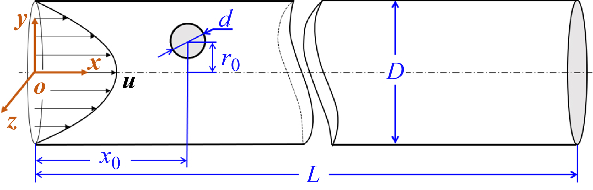
We consider a neutrally buoyant, rigid sphere immersed in a pressure-driven incompressible Newtonian Poiseuille pipe flow, see figure 1. The particle density is identical to that of the fluid,
 $\rho = 1050\,\text{kg}\,\text{m}^{-3}$
, and the kinematic viscosity is
 $\nu = 1.4286\times 10^{-6}\,\text{m}^2\,\text{s}^{-1}$
. The pipe diameter is
 $D=8\,\text{mm}$
and its length
 $L$
= 250
 $D$
= 2 m, sufficient for the sphere to reach equilibrium. The fluid flows in the positive
 $x$
-direction, with a fully developed velocity profile imposed at the inlet. The corresponding velocity and pressure fields for fully developed circular Poiseuille flow are
 \begin{align} u(r) &= 2\bar {u}\left [1 - \left (\frac {2r}{D}\right )^2\right ], \end{align}
 \begin{align} p(x) &= \lambda \frac {L-x}{D} \, \frac {\rho \,\bar {u}^2}{2}, \end{align}
where
 $u(r)$
is the axial velocity at radial position
 $r$
,
 $\bar {u}$
the mean velocity and
 $\lambda = 64/Re$
is the resistance coefficient. The axial pressure
 $p(x)$
drives the flow, where
 $x$
is the axial position relative to the inlet.
Schematic of the simulation set-up for inertial migration of a sphere of diameter
 $d$
in a circular pipe of diameter
 $D=8\,\text{mm}$
and length
 $L$
. A fully developed velocity profile is preset at the inlet and the sphere is initially placed at
 $(r_0, x_0=4d)$
.

A constant static pressure of zero is specified at the pipe outlet and a no-slip condition is imposed at the wall. The sphere is initially positioned at radial location
 $r_0$
relative to the pipe axis (
 $r = 0$
) and axial location
 $x_0=4d$
relative to the inlet (
 $x=0$
) (figure 1). The choice of
 $x_0$
was verified to not influence the inertial migration dynamics. Unless otherwise specified, the sphere’s initial axial velocity matches the undisturbed fluid velocity at the sphere centre, while the initial radial and angular velocities of the sphere are both zero.
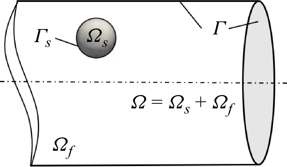
The computational domain (figure 2) is denoted by
 $\varOmega = \varOmega _{{f}} \cup \varOmega _{{s}}$
, where
 $\varOmega _{{f}}$
is the fluid subdomain and
 $\varOmega _{{s}}$
the solid (particle) subdomain. Additionally,
 $\varGamma _{{s}} = \partial \varOmega _{{s}}$
is the solid boundary, that is, the fluid–particle interface, and
 $\varGamma = \partial \varOmega$
is the boundary of the entire domain.
Schematic of the computational domain for a sphere immersed in Poiseuille flow. The fluid domain is denoted by
 $\varOmega _{{f}}$
, the solid (particle) domain by
 $\varOmega _{{s}}$
with boundary
 $\varGamma _{{s}}$
and the total domain by
 $\varOmega = \varOmega _{{f}} \cup \varOmega _{{s}}$
with boundary
 $\varGamma$
.

The flow in the domain
 $\varOmega$
is governed by the continuity and momentum equations (Shirgaonkar, Maciver & Patankar Reference Shirgaonkar, Maciver and Patankar2009):
 \begin{align} \boldsymbol{\nabla }\boldsymbol{\cdot }\boldsymbol{u} &= 0, \end{align}
 \begin{align} \rho \left (\frac {\partial \boldsymbol{u}} {\partial t} + \boldsymbol{u} \boldsymbol{\cdot }\boldsymbol{\nabla }\right ) \boldsymbol{u} &= \boldsymbol{\nabla }\boldsymbol{\cdot }\boldsymbol{\sigma } =\rho \nu {\nabla} ^2 \boldsymbol{u}- \boldsymbol{\nabla }p. \\[9pt] \nonumber \end{align}
Here,
 $\boldsymbol{u}$
is the velocity,
 $\boldsymbol{\mathsf{\sigma }}$
the stress tensor,
 $p$
the pressure,
 $\rho$
the fluid density and
 $t$
the time.
The initial and boundary conditions for the fluid are
 \begin{align} \boldsymbol{u}(t=0)=\boldsymbol{u}_0 \quad & \text{in}\;\quad \varOmega , \end{align}
 \begin{align} \boldsymbol{u}=\boldsymbol{u}_{\varGamma }\,, \quad p= p_\varGamma \quad & \text{on}\;\quad \varGamma. \end{align}
Here,
 $\boldsymbol{u}_0$
is the initial velocity, and
 $\boldsymbol{u}_\varGamma$
and
 $p_\varGamma$
are the specified velocity and pressure at the boundary
 $\varGamma$
.
The effect of the solid domain occupied by the sphere can be expressed as (Shen et al. Reference Shen, Wang, Huang and Feng2022; Ren et al. Reference Ren, Zhang, Zhang and Lu2023; Li et al. Reference Li, Zhang, Shen and Zhang2024)
 \begin{align} \boldsymbol{u} = \boldsymbol{u}_{p} + \boldsymbol{\omega } \times \big (\boldsymbol{r} - \boldsymbol{r}_{\kern-2pt p}\big ) \quad \text{in}\;\quad \varOmega _{{s}}, \end{align}
 \begin{align} \boldsymbol{F}_{\kern-2.5pt{f-p}} = \oint \limits _{\varGamma _{{s}}}\boldsymbol{\sigma } \boldsymbol{\cdot }\boldsymbol{n}\,\text{d}\varGamma _{{s}} \quad \text{on}\;\quad \varGamma _{{s}}. \end{align}
Here,
 $\boldsymbol{u}_{p}$
is the particle translational velocity,
 $\boldsymbol{\omega }$
its angular velocity,
 $\boldsymbol{r}$
the position vector,
 $\boldsymbol{r}_{\kern-2pt p}$
the particle centroid position,
 $\boldsymbol{F}_{\kern-2.5pt{f-p}}$
the fluid–particle interaction force and
 $\boldsymbol{n}$
is the outward normal unit vector on the particle surface.
In the discrete element method (DEM), the translational and rotational motion of a rigid sphere is governed by Newton’s second law,
 \begin{align} m_{p}\,\frac {\textrm{d}\boldsymbol{u}_{p}}{\textrm{d}t} &= m_{p}\,\boldsymbol{g} + \boldsymbol{F}_{\kern-2.5pt{f-p}}, \end{align}
 \begin{align} I_{p}\,\frac {\textrm{d}\boldsymbol{\omega }}{\textrm{d}t} &= \boldsymbol{T}_{\kern-2.5pt{f-p}}. \end{align}
Here,
 $m_{p}$
is the sphere’s mass,
 $I_{p}$
its moment of inertia and
 $\boldsymbol{g}$
the gravitational acceleration. The hydrodynamic torque,
 $\boldsymbol{T}_{\kern-2.5pt{f-p}}$
, due to fluid–particle interactions is given by (Hager et al. Reference Hager, Kloss, Pirker and Goniva2014; Shen et al. Reference Shen, Wang, Huang and Feng2022; Li et al. Reference Li, Zhang, Shen and Zhang2024)
 \begin{equation} \boldsymbol{T}_{\kern-2.5pt{f-p}} = \int \limits _{\varOmega _{{s}}} \big (\boldsymbol{r} - \boldsymbol{r}_{\kern-2pt p}\big ) \times \big (\rho \nu {\nabla} ^2 \boldsymbol{u} - \boldsymbol{\nabla }p\big ) \, \text{d}\varOmega _{{s}}. \end{equation}
3. Numerical method
The simulations are carried out using a two-way coupled CFD–DEM approach, implemented in the open-source software package CFDEMcoupling (Kloss et al. Reference Kloss, Goniva, Hager, Amberger and Pirker2012). In this framework, the fluid phase is solved with the CFD solver OpenFOAM, while the particle dynamics are computed with the DEM code LIGGGHTS. The fictitious domain method (FDM) is employed to account for the moving boundaries of the sphere by treating the solid sphere as a fictitious fluid region (Shao, Wu & Yu Reference Shao, Wu and Yu2012; Wang, Abbas & Cliement Reference Wang, Abbas and Cliement2017; Xia et al. Reference Xia, Xiong, Yu and Zhu2020). This allows the fluid and particle equations of motion to be fully resolved and consistently coupled through fluid–solid interaction forces.
The computational domain
 $\varOmega$
is initially discretised using hexahedral meshes (figure 3), which provide efficient resolution of the fluid field. A detailed description of the numerical procedure can be found in Appendix A. The downstream length of the simulation domain is set as equal to the pipe length (
 $L$
= 2 m). A maximum mesh size of
 $0.05D$
in the radial direction and a mesh size of
 $0.1D$
in the axial direction are adopted in the simulations, based on the mesh convergence test described in Appendix B. Initially, the simulation domain contains 1 050 000 mesh elements and 1 102 941 nodes. A time step of
 $\Delta t = 1.6 \times 10^{-5}$
s is applied for both CFD and DEM computations, while dynamic mesh refinement is conducted at every iteration of the numerical simulation to capture the fluid–particle interactions with high accuracy (figure 4).
Computational mesh for a circular pipe: (a) zoomed longitudinal section; (b) outlet region; (c) pipe cross-section.

Dynamic mesh refinement used in the simulations to resolve fluid–particle interactions: (a) longitudinal section through the sphere centre; (b) cross-section at the sphere centre. The local refinement ensures accurate resolution of the flow field around the moving sphere.

4. Model validation
The model and numerical method described in §§ 2 and 3 are validated against theoretical predictions for velocity and pressure fields, as well as against published experimental data on equilibrium positions of inertial migration.
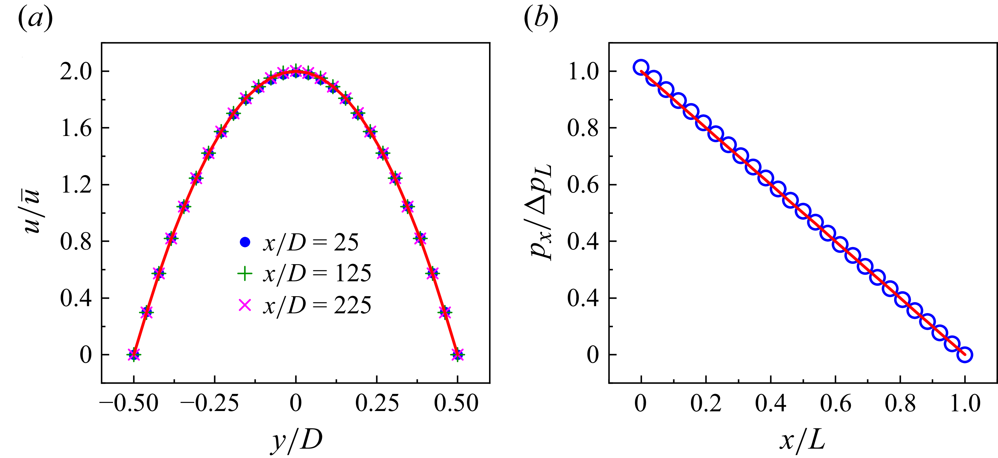
Figure 5(a) shows the steady-state axial velocity profiles across the pipe cross-section,
 $u(y/D)$
, obtained at different axial locations for particle-free flow at
 $Re=256$
. Figure 5(b) shows the corresponding axial pressure distribution. In both cases, the numerical results (symbols) agree closely with the analytical predictions for Poiseuille flow (2.1), (2.2): the velocity profiles are parabolic, while the pressure decreases linearly along the axis. These results confirm the accuracy of the CFD model in predicting the flow field in the absence of particles.
Comparison of numerical and analytical solutions for velocity and pressure profiles: (a) cross-section velocity profiles at
 $x/D=25$
, 125 and 225, with
 $y/D$
denoting the radial coordinate normalised by the pipe diameter; (b) axial pressure profile. The simulations were performed for particle-free flow at
 $Re=256$
in a pipe of length
 $L=250\, D$
. Symbols denote steady-state numerical results, while continuous lines show the analytical solutions from (2.1) and (2.2). Here,
 $\Delta p_L$
is the pressure drop across the full pipe length
 $L$
and
 $p_x$
is the pressure at axial position
 $x$
.

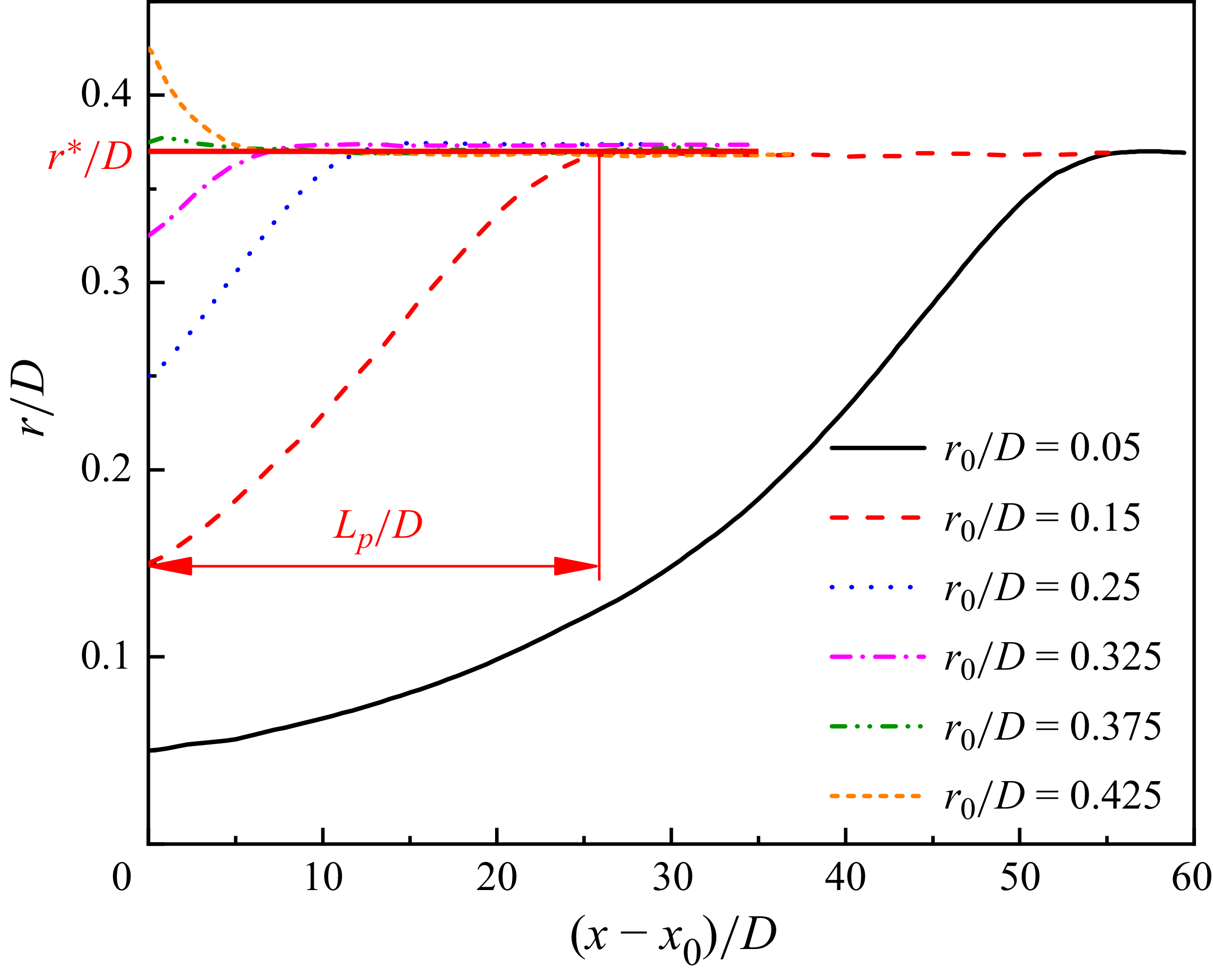
Inertial migration of a neutrally buoyant sphere in circular Poiseuille flow for different initial radial positions,
 $r_0$
. Simulations were performed at
 $Re=256$
and
 $d/D=0.125$
. The normalised length
 $L_{p}/D$
, with
 $L_{p}=x-x_0$
, required to reach the equilibrium radial position,
 $r^\ast$
, is indicated for the case
 $r_0/D=0.15$
.

Next, we consider a sphere in pipe flow at
 $Re=256$
with
 $d/D=0.125$
. The particle trajectories are shown in figure 6. The radial position
 $r/D$
evolves monotonically towards an equilibrium value
 $r^*/D \approx 0.37$
, independent of the initial radial position. This so-called tubular pinch effect arises from inertial migration and agrees with previous experimental (Karnis et al. Reference Karnis, Goldsmith and Mason1966; Nakayama et al. Reference Nakayama, Yamashita, Yabu, Itano and Sugihara-Seki2019) and numerical (Choi & Kim Reference Choi and Kim2010; Pan et al. Reference Pan, Li and Glowinski2021; Aouane et al. Reference Aouane, Sega, Bäuerlein, Avila and Harting2022) studies. The equilibrium value is in quantitative agreement with the experiments by Matas et al. (Reference Matas, Morris and Guazelli2004), who used the same fluid and particle properties, geometry, and Reynolds number. The associated entry length
 $L_{p}$
, defined as the axial distance required for the sphere to reach its equilibrium position, depends on
 $r_0$
, in agreement with previous numerical studies (Aouane et al. Reference Aouane, Sega, Bäuerlein, Avila and Harting2022; Feng et al. Reference Feng, Hu and Joseph1994b
).
For further validation, we vary
 ${\textit{Re}}$
between 57 and 800 for
 $d/D=0.125$
and 0.11, with the particle initially placed at
 $r_0/D=0.25$
. Figure 7 compares the numerically predicted equilibrium positions with experimental data by Matas et al. (Reference Matas, Morris and Guazelli2004) and Morita et al. (Reference Morita, Itano and Sugihara-Seki2017). We achieve quantitative agreement with an absolute deviation of less than 8.8 % and a mean absolute deviation of 2.5 %. As
 ${\textit{Re}}$
increases,
 $r^*/D$
shifts towards the wall, in line with previous numerical observations (Aouane et al. Reference Aouane, Sega, Bäuerlein, Avila and Harting2022). The simulation data in figure 7 can be fitted by an exponential relaxation law,
 \begin{equation} \frac {r^*}{D} = \frac {r^*_\infty }{D} \left \{ 1 - \exp \left [ -\left (\frac {Re}{Re_{{c}}}+\delta \right ) \right ] \right \}, \end{equation}
where the asymptotic radial position,
 $r^*_\infty /D \approx 0.384$
and
 $0.395$
for
 $d/D=0.125$
and
 $0.11$
, respectively. Moreover, the characteristic Reynolds number
 ${\textit{Re}}_{{c}}$
and
 $\delta$
are fit parameters. For
 $d/D = 0.125$
,
 ${\textit{Re}}_{{c}} \approx 110$
and
 $\delta \approx 1.44$
; while for
 $d/D = 0.11$
,
 ${\textit{Re}}_{{c}} \approx 150$
and
 $\delta \approx 1.67$
. While this expression captures the low-
 ${\textit{Re}}$
regime well, deviations appear at higher
 ${\textit{Re}}$
, reflecting the onset of distinct inertial migration regimes discussed later.
Comparison of numerically predicted equilibrium radial positions with experimental data by Matas et al. (Reference Matas, Morris and Guazelli2004) and Morita et al. (Reference Morita, Itano and Sugihara-Seki2017) and the theory by Matas, Morris & Guazelli (Reference Matas, Morris and Guazelli2009): (a) for
 $d/D=0.125$
and (b) for
 $d/D=0.11$
. In the simulations, the initial radial position is
 $r_0/D=0.25$
, however, as shown in figure 6, the asymptotic state is independent of the initial position. The solid lines are a fit of (4.1) to the simulation results.

5. Results
5.1. Inertial migration regimes
In the Stokes limit (
 $Re \to 0$
), a neutrally buoyant sphere starting at
 $r_0/D=0.25$
follows the fluid streamlines with no lateral migration. Inertia alters this behaviour for finite
 ${\textit{Re}}$
. By varying
 ${\textit{Re}}$
between 100 and 800 through increasing the fluid velocity, we identify three distinct regimes of inertial migration. These regimes differ in their dependence on
 ${\textit{Re}}$
, the associated radial dynamics and the particle rotational velocities.
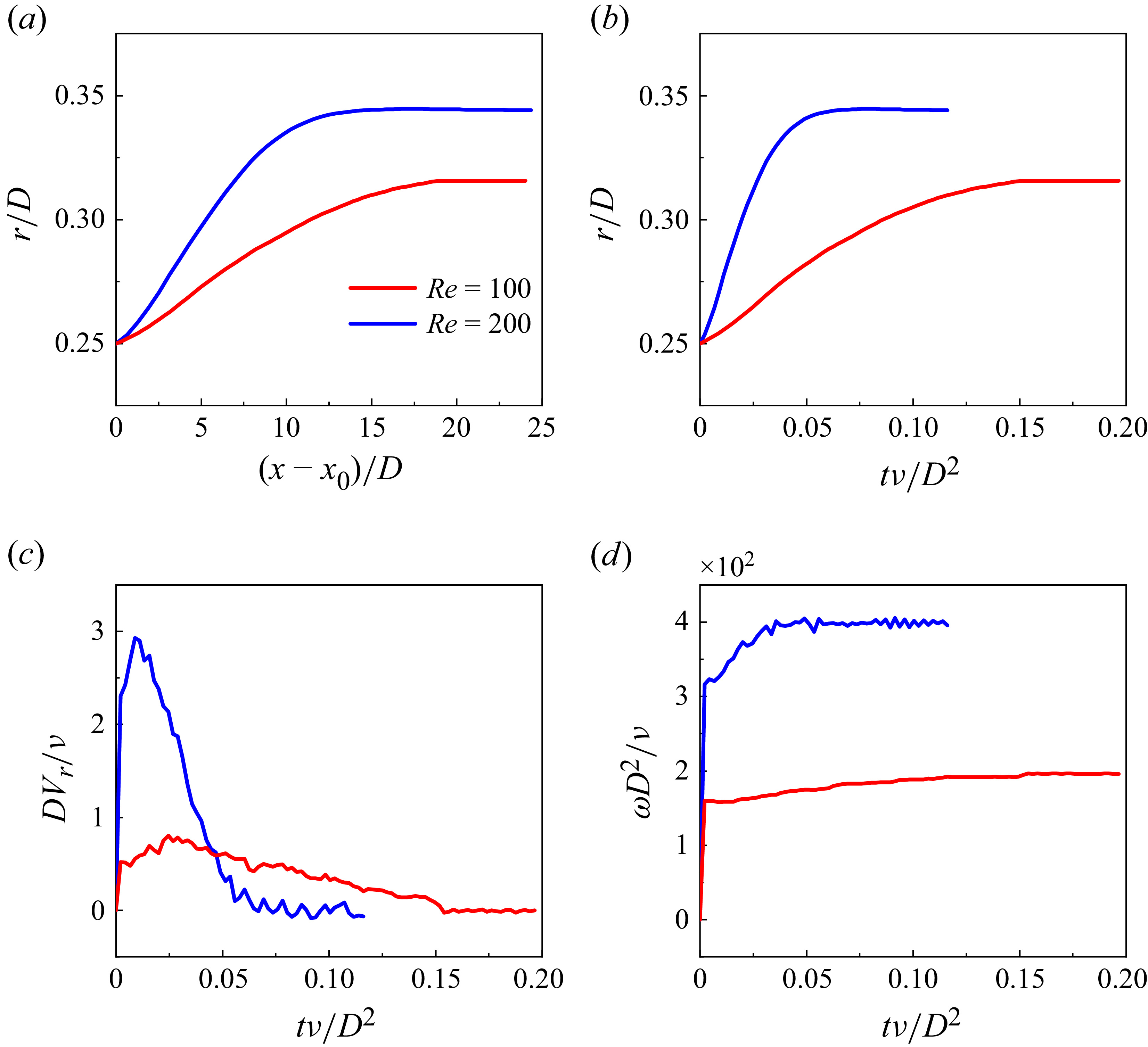
Monotonic regime (figure 8): for
 $Re\lesssim 200$
, the sphere migrates monotonically from its initial radial position
 $r_0/D$
to the equilibrium position
 $r^\ast /D$
. The radial migration velocity first increases and then decays as the sphere approaches its equilibrium position, while the angular velocity rises and saturates when the sphere assumes
 $r^\ast /D$
. Small fluctuations in both quantities are attributed to numerical errors from fluid–particle interactions, which become more pronounced at higher
 ${\textit{Re}}$
.
Monotonic regime for
 $Re\lesssim 200$
. (a) Trajectories for
 $Re\in \{100, 200\}$
; (b)–(d) radial position, radial migration velocity and rotational velocity as functions of dimensionless time. Parameters:
 $d/D=0.167$
,
 $r_0/D=0.25$
. Variation in
 ${\textit{Re}}$
was achieved by changing the flow velocity while keeping the viscosity and pipe diameter fixed.

Overshooting regime (figure 9): for
 $250 \lesssim Re \lesssim 350$
, the sphere overshoots the equilibrium radial position
 $r^*/D$
before eventually relaxing to it. In this regime, both the maximum radial displacement during the overshoot and the radial migration velocity increase with
 ${\textit{Re}}$
. The particle’s rotational velocity likewise exhibits an overshoot before stabilising at a constant value, which depends strongly on
 ${\textit{Re}}$
.
Overshooting regime for
 $250 \lesssim Re \lesssim 350$
. Same variables as in figure 8, but for
 $Re=250$
and
 $300$
(overshooting regime) and
 $Re=350$
(near the transition to the oscillatory regime).

Oscillatory regime (figure 10): at sufficiently high Reynolds numbers (
 $Re \gtrsim 400$
), the overshooting regime transitions to an oscillatory one, where the sphere undergoes damped oscillations about the equilibrium position. Both the maximum oscillation amplitude and the entry length required to reach equilibrium increase with
 ${\textit{Re}}$
, while the rotational velocity exhibits only weak oscillations.


The three regimes are not sharply separated. The transition from monotonic to overshooting migration occurs at
 $Re\approx 200{-}250$
and the overshooting–oscillatory transition at
 $Re\approx 350$
.
The phenomenon resembles the behaviour reported by Feng et al. (Reference Feng, Hu and Joseph1994b
) for the lateral migration of a non-neutrally buoyant circular disc in two-dimensional Poiseuille flow, where monotonic, overshooting and oscillatory migration trajectories were obtained by varying the particle-to-fluid density ratio between 0.85 and 1.1 at
 $Re=60$
and
 $d/D=0.125$
.
5.2. Particle-scale mechanics of inertial migration
To develop a mechanistic understanding of inertial migration, we examine the fluid forces acting on the particle and their impact on the particle trajectory. As noted in previous studies (Liu et al. Reference Liu, Xue, Sun and Hu2016; Zhou & Papautsky Reference Zhou and Papautsky2020; Zhang et al. Reference Zhang, Wang, Onck and Toonder2020; Shi et al. Reference Shi, Rzehak, Lucas and Magnaudet2020; Bai et al. Reference Bai, Jin, Liu, Wang and Zhang2022; Feng et al. Reference Feng, Hu and Joseph1994a
), the particle experiences a shear-gradient lift force,
 $F_{{sg}}$
, arising from the curvature of the Poiseuille velocity profile and directed towards the wall.
A wall-induced lift force,
 $F_{{w}}$
, results from the asymmetry of the near-wall and near-centre flow fields. The velocity lag (slip velocity) between the particle and the surrounding fluid generates a slip-shear (Saffman) lift force,
 $F_{{ss}}$
, while the particle’s rotation gives rise to a Magnus lift force,
 $F_{{M}}$
. These lift forces,
 $F_{{w}}$
,
 $F_{{ss}}$
and
 $F_{{M}}$
, act towards the pipe centre and cause the sphere’s radial inertial migration shown in figures 8, 9 and 10. The total lift force is thus (Liu et al. Reference Liu, Xue, Sun and Hu2016; Su, Zheng & Hu Reference Su, Zheng and Hu2023; Feng et al. Reference Feng, Hu and Joseph1994b
)
 \begin{equation} F_{{L}} = F_{{sg}} - F_{{w}} - F_{{ss}} - F_{{M}}, \end{equation}
with positive values indicating a force directed from the pipe centre towards the wall. Equation (5.1) implies that the lift force is composed of four terms arising from different mechanisms.
The competition among these forces determines the equilibrium position and the migration regime. If the particle is initially away from the wall but not near the axis,
 $F_{{sg}}$
dominates, driving migration towards the wall. In contrast, a particle starting close to the wall experiences dominant
 $F_{{w}}$
and migrates towards the centre. At the equilibrium radial position, the lift forces balance and the sphere finds its asymptotic location.
As
 ${\textit{Re}}$
increases, the curvature of the velocity profile intensifies, thereby enhancing
 $F_{{sg}}$
. Larger slip and rotational velocities increase
 $F_{{ss}}$
and
 $F_{{M}}$
. Larger
 ${\textit{Re}}$
also increases the flow asymmetry felt by the sphere at the wall-faced side and the centre-faced side, strengthening
 $F_{{w}}$
(figure 11).
 $Q$
-criterion fields in a longitudinal section through the sphere centre for different Reynolds numbers at
 $d/D=0.167$
.
 $Q$
is an invariant defined as
 $Q = 0.5(\|\boldsymbol{\varOmega }\|^2 - \|\boldsymbol{S}\|^2)$
, where
 $\|\boldsymbol{\cdot }\|$
denotes the Frobenius norm, while
 $\boldsymbol{\varOmega }$
and
 $\boldsymbol{S}$
are the angular rotation-rate tensor and the strain-rate tensor, respectively (Kovács & Balla Reference Kovács and Balla2025). The fields correspond to the instant when the particle first reaches
 $r/D=0.3$
during migration.

In summary, all lift forces acting on the sphere scale with
 ${\textit{Re}}$
and collectively govern the sphere’s inertial migration. The distinct migration regimes arise from the changing balance of the forces in (5.1) as
 ${\textit{Re}}$
varies.
At
 $Re \lesssim 200$
(monotonic regime), a particle initially at
 $r_0/D=0.25$
experiences only a weak
 $F_{{sg}}$
, resulting in slow lateral migration. In this regime,
 $F_{{ss}}$
and
 $F_{{M}}$
counteract migration towards the wall, while
 $F_{{w}}$
remains negligible due to weak near-wall flow asymmetry (figure 11
a).
At
 $Re \approx 250$
(overshooting regime),
 $F_{{sg}}$
increases substantially and accelerates the particle towards the wall. This acceleration is not fully balanced by
 $F_{{ss}}$
and
 $F_{{M}}$
. Consequently, the sphere acquires a higher radial velocity towards the wall, thus overshooting its equilibrium radial position
 $r^\ast /D$
. As the particle moves past equilibrium,
 $F_{{w}}$
becomes significant and restores it towards the centre, but without inducing a second overshoot; instead,
 $r/D$
approaches
 $r^\ast /D$
asymptotically (figure 9
a).
At
 $Re \gtrsim 400$
(oscillatory regime), the particle overshoots
 $r^\ast /D$
multiple times, with the number of oscillations increasing with
 ${\textit{Re}}$
. Oscillations arise because inward-directed forces (
 $F_{{w}}+F_{{ss}}+F_{{M}}$
) dominate for
 $r/D \gt r^\ast /D$
, while
 $F_{{sg}}$
(pointing towards the wall) dominates for
 $r/D \lt r^\ast /D$
. The oscillation amplitude decays due to viscous damping by drag.
The balance of lift forces also explains the dependence of
 $r^\ast /D$
on
 ${\textit{Re}}$
seen in figure 7. In the monotonic regime,
 $r^\ast /D$
increases with
 ${\textit{Re}}$
, but saturates for
 $Re \gtrsim 250$
. The location of the stable position is, thus, insensitive to
 ${\textit{Re}}$
in the overshooting and oscillatory regimes. This saturation occurs when inward-directed lift forces balance
 $F_{{sg}}$
at a nearly constant
 $r^\ast /D$
. While earlier studies also reported saturation of the radial equilibrium position as a function of the Reynolds number, our simulations show this saturation arises in the overshooting and oscillatory regimes of inertial migration and is associated with the balance of the contributing forces.
The overshooting and oscillatory migration regimes originate from the finite inertia of the fluid–particle system, which includes the contribution of added-mass effect. In the oscillatory regime, the mean radial position of the particle, around which the trajectory displays oscillatory behaviour, is close to the equilibrium position. However, despite the mean radial position of oscillations corresponding to an approximate balance of lift forces, the particle can overshoot the radial equilibrium position owing to inertial effects. This overshoot leads to a reversal in the direction of lift and, thus, to a reversal in the radial motion of the particle. The dynamics is associated with a force field that alternates between the inward and outward directions, thereby leading to a damped oscillation that progressively decays due to viscous dissipation.
5.3. Role of sphere-to-pipe diameter ratio on the inertial migration regimes
We performed simulations with different sphere diameters
 $d$
while keeping the pipe diameter fixed at
 $D=8$
mm to study the influence of the sphere-to-pipe diameter ratio
 $d/D$
. Figure 12 shows the trajectories for
 $200\le Re \le 800$
.
Particle migration trajectories at different Reynolds numbers. Results are shown for (i)
 $d/D=0.083$
, (ii) 0.1, (iii) 0.125, (iv) 0.167 and (v) 0.25.

Both threshold Reynolds numbers separating the regimes decrease with
 $d/D$
, thus, larger particles transition between regimes at lower
 ${\textit{Re}}$
. This trend arises because the lift forces,
 $F_{{sg}}$
(shear-gradient),
 $F_{{w}}$
(wall-induced),
 $F_{{ss}}$
(slip-shear) and
 $F_{{M}}$
(rotation-induced), scale with the particle size. Consequently, the net lift force grows with
 $d$
, shifting the regime boundaries to lower
 ${\textit{Re}}$
.
Figure 12 also shows that the equilibrium radial position shifts towards the pipe axis as
 $d/D$
increases, largely independent of
 ${\textit{Re}}$
. This trend arises because the equilibrium position reflects a balance of inward- and outward-directed lift forces, while the inward wall-induced lift
 $F_{{w}}$
grows more strongly with
 $d/D$
than the outward shear-gradient force
 $F_{{sg}}$
. Thus, larger particles experience a stronger wall-repelling effect, which shifts the equilibrium position towards the pipe’s centreline.
It should be emphasised that this study aims at improving our fundamental understanding of the Segré–Silberberg effect, rather than focusing on a specific application. This understanding must incorporate oscillatory situations of particle migration associated with spatial changes in flow conditions – the length scale of which is dictated by the entry length. Indeed, the Segré–Silberberg effect has a very broad range of applications throughout a spectrum of flow length scales. The practical importance of the Segré–Silberberg effect is, thus, unquestionable, with applications that include, for instance, microfluidic processes for particle sorting, counting, and separation by size and shape in channels of various dimensions and geometric shapes. Depending on the Reynolds number and the sphere-to-pipe diameter ratio, oscillatory migration behaviour becomes an intrinsic aspect of the flow transport process, with potential implications for various fields, from diagnostics and cell/biomolecule manipulation to proppant transport in oil. As well noted by Di Carlo et al. (Reference Di Carlo, Irimia, Tompkins and Toner2007) and Park, Lee & Kim (Reference Park, Lee and Kim2025), the capability of accurately predicting particle trajectories is indispensable for the efficient and precise particle manipulation in practical applications.
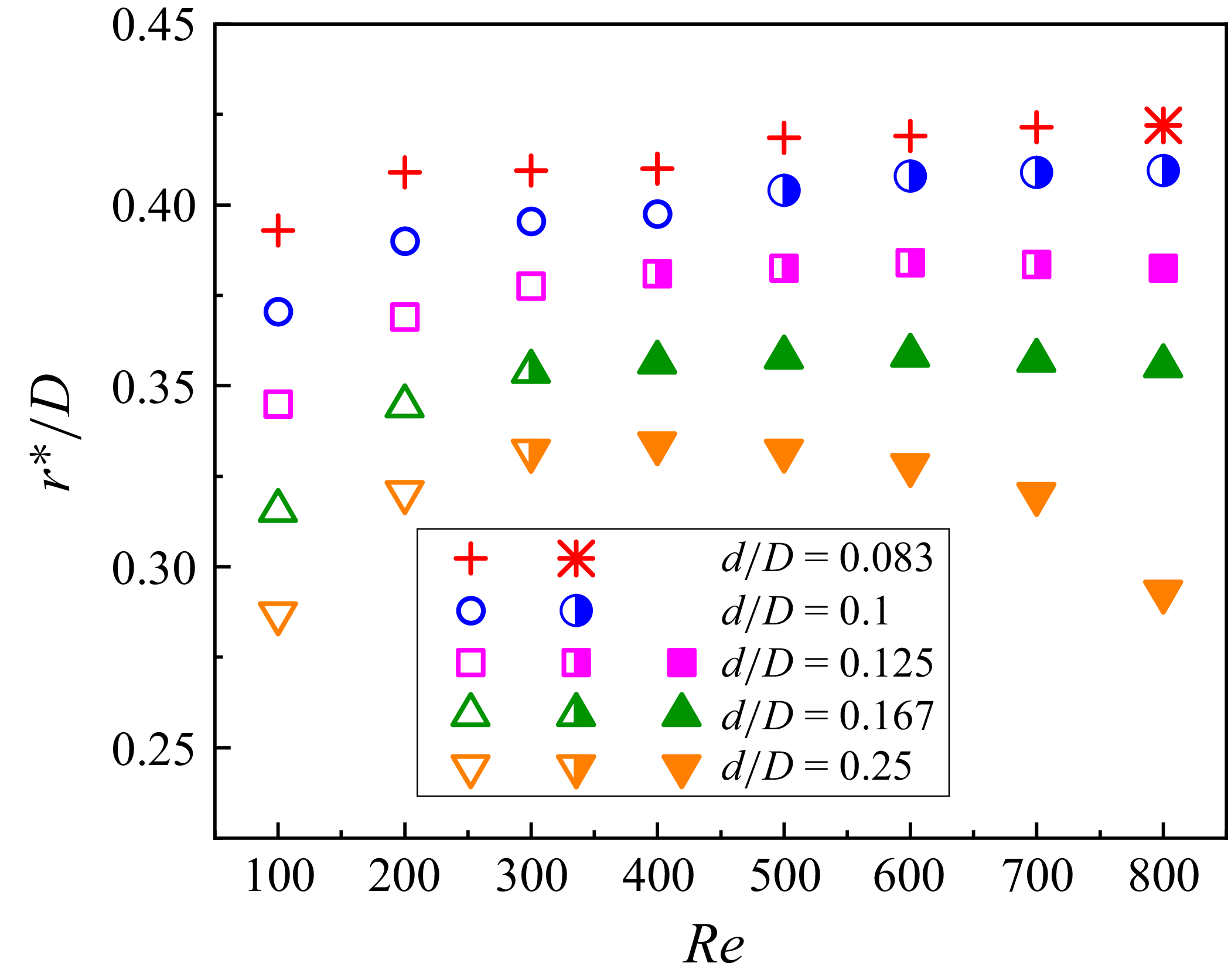
Figure 13 summarises the dependence of the equilibrium radial position
 $r^\ast /D$
on the sphere-to-pipe diameter ratio
 $d/D$
and Reynolds number
 ${\textit{Re}}$
. It is worth noting that the migration behaviour is independent of the particle’s initial position and initial conditions, as detailed in Appendix C. The migration regimes are distinguished by the symbol filling, as explained in the caption. In the monotonic regime,
 $r^\ast /D$
increases with
 ${\textit{Re}}$
, consistent with the matched asymptotic theory (Asmolov Reference Asmolov1999; Matas et al. Reference Matas, Morris and Guazelli2009).
Variation of the equilibrium radial position
 $r^\ast /D$
with
 ${Re}$
. For each value of
 $d/D$
, we indicate the transition between the regimes by modifying the symbol. The cross (
 $+$
) and open symbols, monotonic regime;
 $\ast$
and half-filled, overshooting regime; filled symbols, oscillatory regime. All simulations start at
 $r_0/D=0.25$
.

Once the overshooting regime is reached and even more in the oscillatory regime,
 $r^\ast /D$
shifts progressively towards the pipe’s centre as
 ${\textit{Re}}$
increases. This inward shift is much more pronounced for the largest particles (
 $d/D=0.25$
) than for intermediate ones (
 $d/D=0.167$
), reflecting the growing influence of particle inertia in the oscillatory regime. At Reynolds numbers approaching
 $10^3$
, nonlinear effects associated with the transition from laminar to turbulent flow are expected to become increasingly important and should be addressed in future work. Overall, figure 13 demonstrates that the tubular pinch effect depends jointly on
 ${\textit{Re}}$
and
 $d/D$
, providing further insight into the physics of the different inertial migration regimes.
To characterise the oscillatory behaviour of inertial migration, we model the sphere’s oscillatory motion as a damped harmonic oscillator and find that the theoretically calculated oscillation periods agree reasonably with those obtained from numerical simulations, as detailed in Appendix D. We thus conclude that the damped harmonic oscillator can be regarded, to first order, as a model for the mechanics of the radial motion of the particle in the oscillatory regime.
To give insights into the sphere’s rotation at equilibrium, the final rotational velocity is normalised by the undisturbed fluid velocity gradient at the sphere centre, as detailed in Appendix E. We note that the normalised rotational velocities are consistently smaller than 0.5, the value for a non-inertial, neutrally buoyant sphere in linear shear flow. Furthermore, these velocities decrease with increasing
 ${\textit{Re}}$
and
 $d/D$
, indicating that inertial effects play an increasingly important role as both parameters rise.
We note that Shao et al. (Reference Shao, Yu and Sun2008) and Nakayama et al. (Reference Nakayama, Yamashita, Yabu, Itano and Sugihara-Seki2019) reported the occurrence of a discontinuous jump from the outer equilibrium point to the inner equilibrium point (or two equilibrium points) in the range of parameters studied in our work, as the Reynolds number increases. By contrast, we have not observed any discontinuous jump from one equilibrium position to another in our numerical simulations. We have performed additional simulations at different initial positions using finer mesh elements and observed that the inertial migration behaviour and the equilibrium radial position remain almost unchanged with respect to the mesh structure applied. Further details regarding the additional simulations can be found in Appendix B.
However, we hypothesise that the discrepancy between our results and those of Shao et al. (Reference Shao, Yu and Sun2008) and Nakayama et al. (Reference Nakayama, Yamashita, Yabu, Itano and Sugihara-Seki2019) lies in the different physical configurations of particle-laden pipe flow considered. Shao et al. (Reference Shao, Yu and Sun2008) numerically observed the presence of two equilibrium positions at
 $d/D = 0.15$
for
 $1000 \le Re \le 1300$
when using a short periodic pipe with a length-to-diameter ratio of
 $L/D = 1$
in their numerical simulations. Their results indicated that the final equilibrium position of the particle depends on its initial location. However, when a periodic pipe with
 $L/D = 2$
was used, the particle released from different initial positions consistently migrated to the same equilibrium position (Shao et al. Reference Shao, Yu and Sun2008). Therefore, the two equilibrium positions may result from hydrodynamic interactions as the particle crosses the boundary.
Moreover, Nakayama et al. (Reference Nakayama, Yamashita, Yabu, Itano and Sugihara-Seki2019) experimentally observed that particles focused on two annuli when
 ${\textit{Re}}$
was between 750 and 830, and explained this phenomenon by analysing the numerically obtained lateral (radial) force as a function of radial position. In their study, a pipe diameter of
 $0.6\,{\textrm{mm}}$
and particle diameters of approximately
 $0.06\,{\textrm{mm}}$
were employed. Therefore, the dimensions of the particles and the pipe were much smaller than those applied in our simulations. The lift forces are affected not only by
 ${\textit{Re}}$
and
 $d/D$
, but also by geometrical parameters such as
 $d$
and
 $D$
. The complexity of the lift forces may alter the force balance at different combinations of
 $d$
and
 $D$
, even when
 $d/D$
remains constant, potentially shifting the equilibrium position as a result.
In summary, while we have found that the discrepancy between our numerical simulations and the results reported by Shao et al. (Reference Shao, Yu and Sun2008) and Nakayama et al. (Reference Nakayama, Yamashita, Yabu, Itano and Sugihara-Seki2019) could not be attributed to mesh resolution, further work is needed to elucidate such discrepancy by considering, in particular, the role of the geometric dimensions of the system. Our simulations focus on a single sphere released into a fully developed Poiseuille flow within a circular pipe of length
 $L = 250D = 2\,{\textrm{m}}$
, thereby excluding both hydrodynamic interactions between particles and entrance effects. Future work should investigate the potential role of such interactions for the observation of a single equilibrium position, as well as in the migration regimes of particles as a function of the Reynolds number, building on the analysis presented in this work.
5.4. Entry length of inertial migration
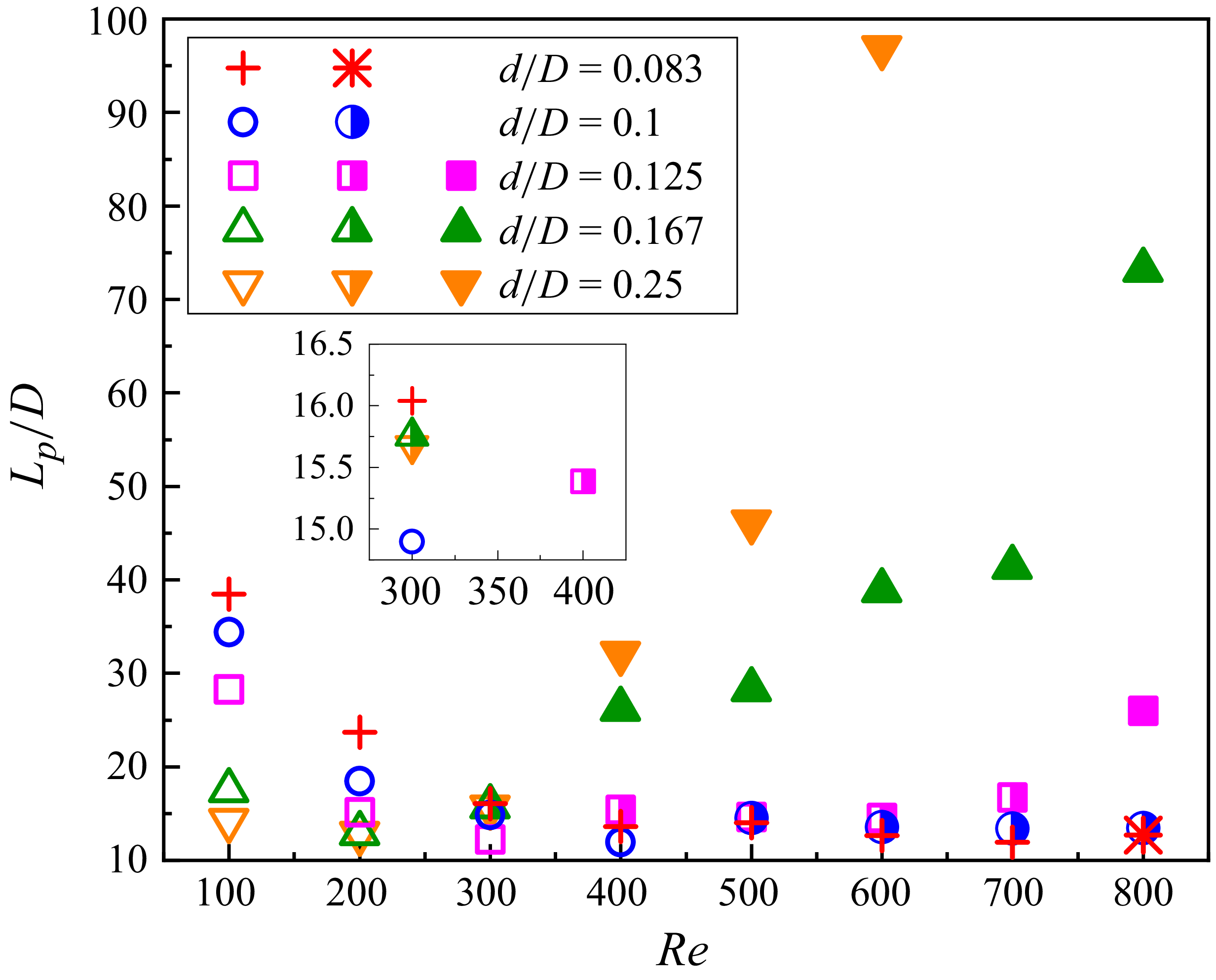
From figure 12, it is evident that the entry length for inertial migration depends on both
 $d/D$
and
 ${\textit{Re}}$
. In the monotonic regime,
 $L_{p}$
decreases with increasing
 $d/D$
, whereas in the overshooting and oscillatory regimes, it increases with
 $d/D$
.
Matas et al. (Reference Matas, Morris and Guazelli2004) developed a theoretical model for
 $L_{p}$
based on matched asymptotic theory, assuming a balance between the lateral lift force
 $F_{{L}}$
and the Stokes drag
 $F_{{d}}$
throughout the migration process until equilibrium is reached. The force balance reads
 \begin{equation} \frac {1}{4} C_{{L}}\left (\frac {d}{D}\right )^4\rho \bar {u}^2 D ^2 =3\pi \nu \rho {d} V_r, \end{equation}
where the left-hand side represents the lift force
 $F_{{L}}$
and the right-hand side the Stokes drag
 $F_{{d}}$
. The coefficient
 $C_{{L}}$
scales the lift force and depends on
 ${\textit{Re}}$
. From this balance, Matas et al. (Reference Matas, Morris and Guazelli2004, Reference Matas, Morris and Guazelli2009) obtained
 \begin{equation} \frac {L_{p}}{D} \approx 6 \pi C_{{L}}^{-1} Re^{-1} \left (\frac {d}{D}\right )^{-3}. \end{equation}
Using matched asymptotic theory to analyse the lateral force on the particle, they showed that
 \begin{equation} C_{{L}} \approx 31.68\,Re^{-0.84}\quad \text{for}\; \quad 50 \le Re \le 1750. \end{equation}
Substituting this expression into (5.3) yields a predictive relation for the entry length
 $L_{p}$
.
Our simulations show that, in the monotonic regime, the sphere migrates towards its equilibrium position with nearly constant radial velocity – except when it is released very close to the pipe axis (see
 $r_0/D=0.05$
in figure 6). Such constant radial migration is consistent with the force-balance assumption of Matas et al. (Reference Matas, Morris and Guazelli2004, Reference Matas, Morris and Guazelli2009), which forms the basis of their trajectory model in the monotonic regime. By contrast, in the overshooting and oscillatory regimes, the migration velocity varies with time and radial position. Moreover, as shown in figure 6 and reported by Aouane et al. (Reference Aouane, Sega, Bäuerlein, Avila and Harting2022), the initial radial position strongly influences the entry length
 $L_{p}$
. This effect is, however, not captured by (5.3).
We therefore propose an extension of (5.3) that incorporates the initial radial position to improve the predictive power of the entry length
 $L_{p}$
in the monotonic regime. For a particle migrating from its initial position
 $r_0$
towards the equilibrium position
 $r^\ast$
(with
 $r_0 \leq r^\ast$
, i.e. outward motion), we have
 \begin{equation} \frac {1}{4}C_{{L}}\left (\frac {d}{D}\right )^{\!4}\rho \bar {u}^2 D ^2 = 3\pi \nu \rho d \frac {\text{d}r}{\text{d}t}. \end{equation}
Thus, we obtain
 \begin{equation} \frac {\text{d}r}{\text{d}t} = \frac {C_{{L}} Re\,\bar {u}}{12\pi }\left (\frac {d}{D}\right )^{\!3}. \end{equation}
Using the undisturbed flow velocity from (2.1), to represent the sphere’s axial velocity,
 $\text{d}x/\text{d}t$
, we can write
 \begin{equation} \frac {\text{d}x}{\text{d}r} = \left .\frac {\text{d}x}{\text{d}t} \right / \frac {\text{d}r}{\text{d}t} =24\pi C_{{L}}^{-1} Re^{-1} \left (\frac {d}{D}\right )^{-3} \left (1-\frac {4r^2}{D^2}\right ). \end{equation}
Integration of (5.7) yields
 \begin{equation} L_{p} = 24\pi C_{{L}}^{-1} Re^{-1} \left (\frac {d}{D}\right )^{-3} \int \limits _{r_0}^{r^*} \left (1-\frac {4r^2}{D^2}\right )\,\text{d}r. \end{equation}
Thus, we obtain
 \begin{equation} \frac {L_{p}}{D} = 24\pi C_{{L}}^{-1} Re^{-1} \left (\frac {d}{D}\right )^{-3} \left [\frac {r^*-r_0}{D} - \frac {4(r^{*3}-r_0^3)}{3 D^3}\right ]\!. \end{equation}
For inward migration, where a particle moves from an initial position
 $r_0 \gt r^\ast$
towards the equilibrium position, the expression becomes
 \begin{equation} \frac {L_{p}}{D} = 24\pi C_{{L}}^{-1} Re^{-1} \left (\frac {d}{D}\right )^{-3} \left [\frac {r_0-r^*}{D} - \frac {4(r_0^3-r^{*3})}{3 D^3}\right ]\!. \end{equation}
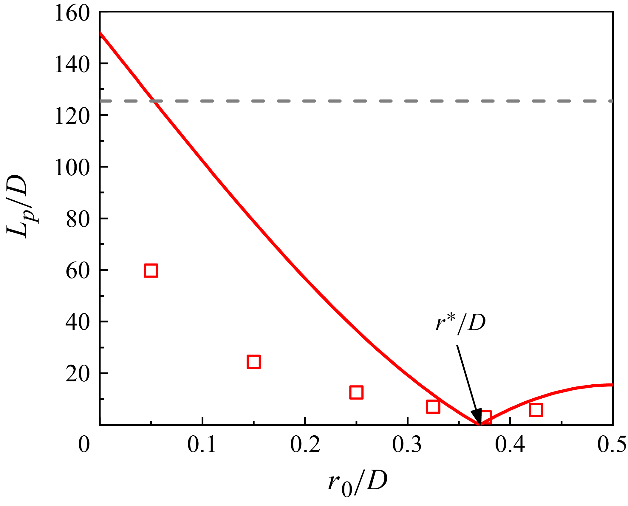
Figure 14 shows the dimensionless entry length
 $L_{p}/D$
as a function of the initial radial position
 $r_0/D$
, obtained from our simulations together with the analytical solutions given by (5.9) and (5.10). For comparison, the prediction of Matas et al. (Reference Matas, Morris and Guazelli2009), as given by (5.3), is also included. As evident from the figure, our model reproduces the numerically observed trend that
 $L_{p}$
decreases as
 $\left | r_0{-}r^\ast \right |$
becomes smaller. The discrepancy between theory and simulation grows as the particle is released closer to the pipe axis, reflecting that the force-balance assumption is only approximately valid near the equilibrium position and breaks down as
 $r_0$
approaches the symmetry axis.
Comparison of the dimensionless entry length
 $L_{p}/D$
from simulations (squares, cf. figure 6) with theoretical predictions: dashed line, (5.3) based on matched asymptotic theory by Matas et al. (Reference Matas, Morris and Guazelli2009); solid line, extended theory (5.9) and (5.10). Simulations and theoretical models use
 $Re=256$
and
 $d/D=0.125$
.

The extended model applies to low Reynolds numbers within the monotonic regime of inertial migration. In this regime,
 $L_{p}/D$
decreases with both
 ${\textit{Re}}$
and
 $d/D$
(see (5.9), (5.10)), since larger
 ${\textit{Re}}$
or
 $d/D$
increases the radial lift force and hence the migration velocity. When the system enters the oscillatory regime,
 $L_{p}$
increases with
 ${\textit{Re}}$
because the oscillation amplitude grows with Reynolds number, resulting in the opposite trend as in the monotonic regime.
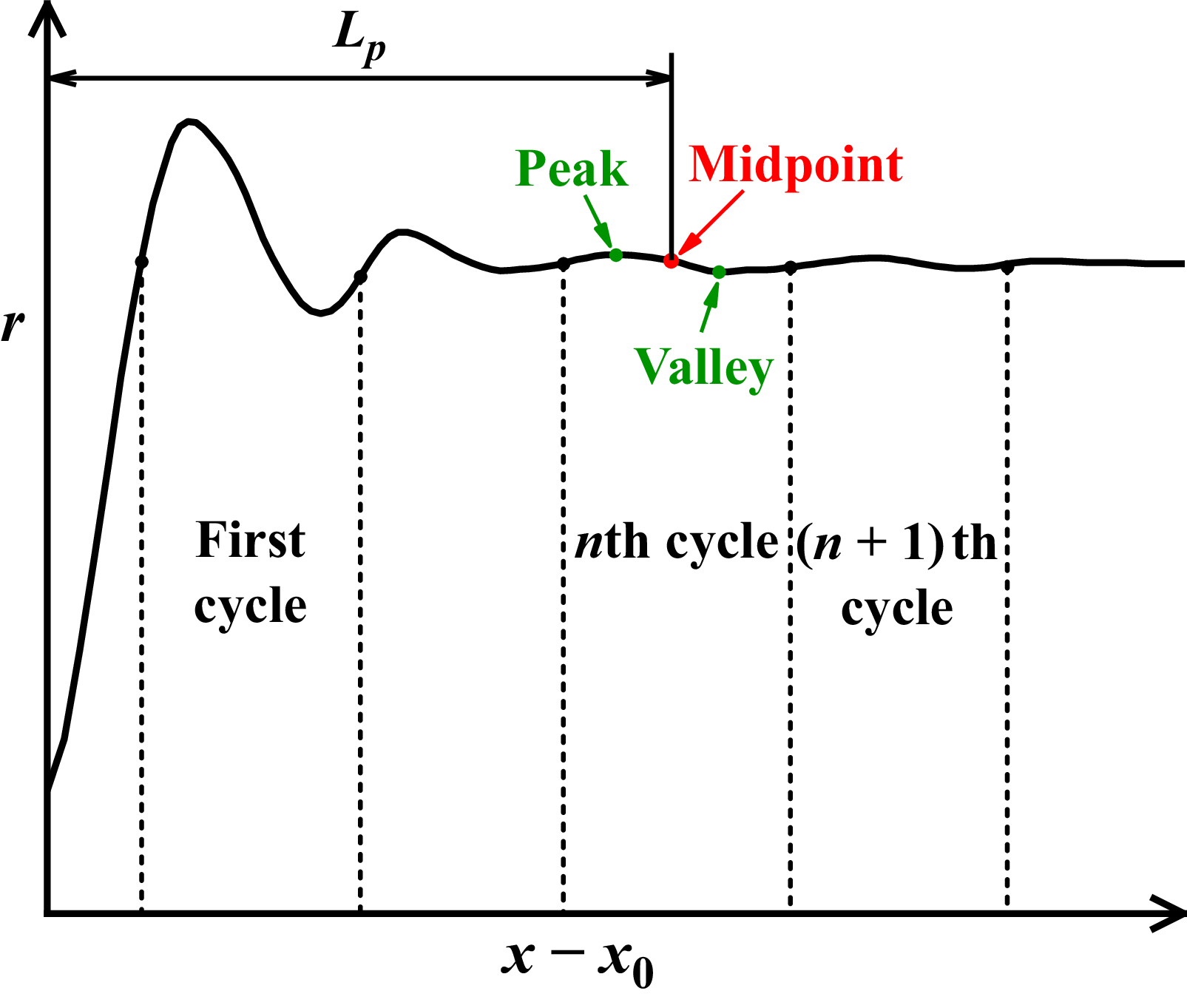
To determine
 $L_{p}$
in the oscillatory regime, we evaluate the relative deviation
 $\delta _n$
of the radial position between successive peak–valley pairs of the migration trajectory. Migration is considered complete when
 $\delta _n \leq 1\,\%$
, and
 $L_{p}$
is defined as the axial distance from the initial position to the midpoint between the corresponding peak and valley. Figure 15 illustrates the procedure.
Illustration of the procedure used to determine the entry length in the oscillatory regime.

Figure 16 shows the dimensionless entry length
 $L_{p}/D$
as a function of Reynolds number across the different migration regimes for various sphere-to-pipe diameter ratios. Note that the values of
 $L_{p}/D$
at
 $Re=700$
and 800 for the largest particle (
 $d/D=0.25$
) are not included, since at high
 ${\textit{Re}}$
, the migration enters the oscillatory regime where oscillations are strong and decay extremely slowly (figure 12
f), making
 $L_{p}$
difficult to determine.
Variation of the entry length
 $L_{p}/D$
with
 ${\textit{Re}}$
for different
 $d/D$
across the migration regimes. Crosses (+) and open symbols denote the monotonic regime, asterisks (
 $\ast$
) and half-filled symbols the overshooting regime, and filled symbols the oscillatory regime. The inset shows an enlarged view of the range
 $14.75 \leq L_{p}/D \leq 16.5$
and
 $275 \leq Re \leq 425$
. Simulations were performed with
 $r_0/D=0.25$
.

The simulation results in figure 16 are consistent with theoretical expectations: in the monotonic regime,
 $L_{p}$
decreases with increasing
 ${\textit{Re}}$
and
 $d/D$
, in agreement with the predictions of (5.9) and (5.10). By contrast, in the oscillatory regime
 $L_{p}$
increases with
 ${\textit{Re}}$
and
 $d/D$
, while the overshooting regime marks a transition between these two opposite trends. These findings highlight that the distinct dynamics of the different inertial migration regimes must be considered in future work to accurately predict
 $L_{p}$
.
Note that the results shown in figure 16 correspond to the case where the particle is initially positioned at
 $r_0/D=0.25$
, which is the midpoint between the pipe wall and the centreline. As observed from figure 14 (and figure 6), the entry length depends on the initial radial position relative to the pipe diameter,
 $r_0/D$
. This dependence is still incompletely understood. Figure 16 further elucidates the entry length at various
 ${\textit{Re}}$
and
 $d/D$
using a fixed
 $r_0/D$
. Consistently with our expectation, our simulations reveal distinct dependences of entry length on
 ${\textit{Re}}$
and
 $d/D$
for different migration regimes. However, state-of-the-art theory for the entry length as a function of
 $r_0/D$
,
 ${\textit{Re}}$
and
 $d/D$
fails to reproduce the results from our simulations by a large amount (see figures 14 and 16). Therefore, numerical simulations like the ones presented in this section are of crucial importance as starting point for future modelling.
Furthermore, we emphasise that the conclusions on the migration regimes, particle-scale mechanics and role of
 $d/D$
on migration regimes presented in §§ 5.1–5.3, respectively, are robust with respect to the value of
 $r_0/D$
. This is attributed to the fact that the migration regimes are insensitive to the particle’s initial position, as presented in Appendix C. Moreover, one of the main findings in § 5.4 is the dependence of the entry length on
 ${\textit{Re}}$
and on
 $d/D$
at a fixed initial position (see figure 16), which is associated with the migration regimes and thus not affected by the initial position. This can be seen from the results presented in Appendix C. Therefore, all main conclusions about the inertial migration dynamics drawn from the results obtained for
 $r_0/D = 0.25$
are valid for all non-zero values of
 $r_0/D$
, with implications for future studies.
6. Conclusions
We conducted a numerical investigation of the inertial migration of a single neutrally buoyant, rigid sphere in fully developed circular Poiseuille flow using the CFD–DEM approach. The undisturbed fluid field and the particle migration behaviour were validated against the analytical solution of Poiseuille flow and experimental data for the equilibrium radial position available in the literature. Following validation, simulations were performed for Reynolds numbers in the range
 $100 \leq Re \leq 800$
and sphere-to-pipe diameter ratios
 $0.083 \leq d/D \leq 0.25$
.
Our results reveal three distinct regimes of inertial migration governed by
 ${\textit{Re}}$
. At low
 ${\textit{Re}}$
, a monotonic regime is observed, where the sphere migrates directly towards its equilibrium position without overshooting. At intermediate
 ${\textit{Re}}$
, migration transitions to an overshooting regime, where the particle overshoots the equilibrium once before asymptotically approaching it. At higher
 ${\textit{Re}}$
, an oscillatory regime emerges, characterised by damped oscillations around the equilibrium. The regime transitions are dictated by the relative balance between the outward shear-gradient lift force and the inward wall-induced, slip-shear and rotation-induced lift forces. In addition,
 $d/D$
plays a central role: increasing
 $d/D$
lowers the critical Reynolds numbers separating the regimes, due to the stronger lift forces acting on larger particles.
The entry length
 $L_{p}/D$
required for full migration also depends strongly on the regime. In the monotonic regime,
 $L_{p}/D$
decreases with both
 ${\textit{Re}}$
and
 $d/D$
, in qualitative agreement with theoretical predictions. In contrast, in the oscillatory regime,
 $L_{p}/D$
increases with
 ${\textit{Re}}$
and
 $d/D$
, reflecting the growth of oscillation amplitude with flow speed and particle inertia, which delays relaxation to the equilibrium position. These findings highlight the importance of accounting for regime-dependent dynamics when modelling the entry length associated with the tubular pinch effect. Future work should, moreover, extend the present study to higher Reynolds numbers and address the influence of turbulence, which is expected to alter both the migration regimes and the associated entry lengths.
Acknowledgements
Support from High Performance Computing Centre at University of Shanghai for Science and Technology is greatly acknowledged. The authors also would like to thank Professor Cameron Tropea at Technische Universität Darmstadt, Germany for enlightening discussions.
Funding
This work was supported by the National Natural Science Foundation of China (grant number 52476157) and the High-end Foreign Expert Introduction Program (Grant No. 2022013002).
Declaration of interests
The authors report no conflict of interest.
Appendix A. Numerical procedure
The coupled CFD-DEM simulation is performed using the cfdemSolverIB solver (Kloss et al. Reference Kloss, Goniva, Hager, Amberger and Pirker2012; Hager Reference Hager2014). The overall solution procedure follows the subsequent workflow (see also figure 17).
-
(i) Initialise the fluid velocity and pressure fields for the CFD domain
 $\varOmega$
, and set the initial position and velocity for the particle in the DEM simulation.
-
(ii) The DEM solver accesses the information of the particle and transfers it to the ‘coupling’ toolbox.
-
(iii) A ‘location model’ within the ‘coupling’ toolbox sets the CFD mesh elements associated with the particle volume according to its position (as determined in the DEM simulation), whereupon the void fraction in each mesh element occupied by the particle is computed; the corresponding solid domain
$\varOmega _{{s}}$
is thereby identified as a fictitious fluid region. -
(iv) The mesh elements within the solid domain
$\varOmega _{{s}}$
occupied by the particle are refined. -
(v) The fluid pressure and velocity fields within the fictitious fluid region computed by the CFD solver are transferred to the DEM solver in the form of a fluid–particle interaction force,
$\boldsymbol{F}_{\kern-1.5pt f-p}$
, and a corresponding torque,
$\boldsymbol{T}_{\kern-1.5pt f-p}$
. -
(vi) The DEM solver computes the translational and rotational motion of the particle in a time step
$\Delta t$
. The values of particle position and velocity are then updated, and the time of DEM simulation
$t_{\textit{DEM}}$
advances
$\Delta t$
. -
(vii) The CFD solver computes the continuity and momentum equations across the computational domain
$\varOmega$
using the PISO algorithm. It then corrects the flow field of the computational domain
$\varOmega$
by incorporating the particle velocity within the fictitious fluid region from the ‘coupling’ toolbox. The time of CFD simulation
$t_{\textit{CFD}}$
advances
$\Delta t$
. -
(viii) Steps (ii)–(vii) are repeated until the time reaches the value of
$t_{end}$
defined in the simulation script.


Workflow of the numerical simulation.

Appendix B. Mesh convergence test
To verify the accuracy of our numerical simulations, we performed a mesh convergence test by taking as reference the case
 $Re = 600$
,
 $d/D = 0.167$
and
 $r_0/D = 0.25$
. Specifically, we considered five different mesh configurations, including
 $1.05$
million initial mesh elements with maximum dynamic mesh refinement levels of
 $0$
,
 $1$
,
 $2$
and
 $3$
, as well as
 $2.10$
million initial mesh elements with a maximum dynamic mesh refinement level of
 $3$
. During the mesh refinement, hexahedral mesh elements were split using an octree structure, with a refinement level associated with each cell as described by Hager et al. (Reference Hager, Kloss, Pirker and Goniva2014).
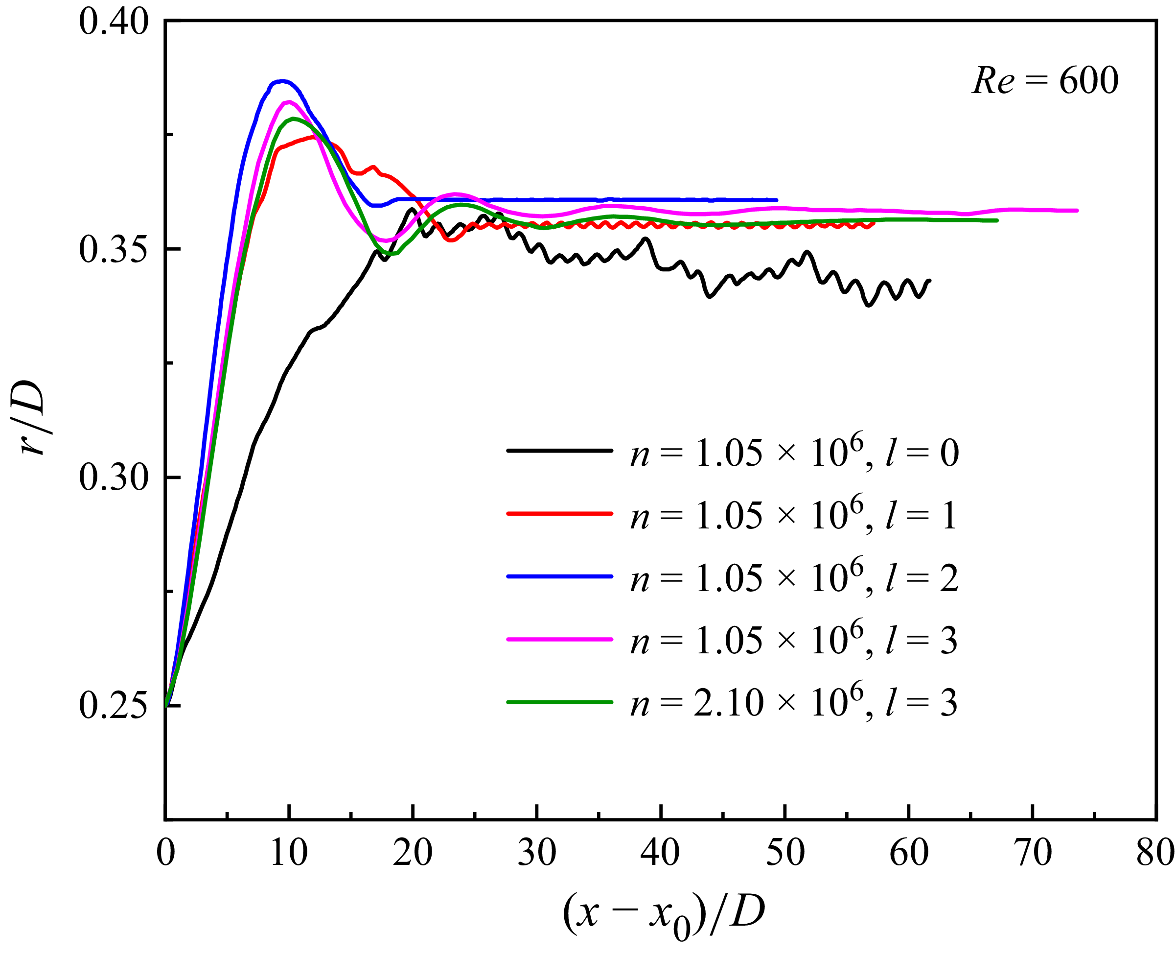
Figure 18 presents the inertial migration trajectory of a neutrally buoyant sphere in circular Poiseuille flow for different initial mesh element numbers and dynamic mesh refinement levels. As shown in figure 18, as the number of initial mesh elements and the maximum refinement level increase, the particle trajectory becomes smoother and a convergence of the simulation results can be observed. In particular, at the maximum refinement level of
 $3$
, the simulation with
 $1.05$
million initial mesh elements is associated with a normalised equilibrium position of
 $r^{*}/D = 0.358$
and a normalised entry length of
 $L_p/D = 38.878$
, while the simulation with
 $2.10$
million initial mesh elements yields
 $r^{*}/D = 0.356$
and
 $L_p/D = 40.115$
. The relative deviations of
 $r^{*}/D$
and
 $L_p/D$
between the simulation results are
 $0.56\,\%$
and
 $3.0\,\%$
, respectively, indicating that the mesh configuration with
 $1.05$
million initial mesh elements and a maximum refinement level of
 $3$
is a good choice to achieve acceptable accuracy at reasonable computational cost.
Inertial migration of a neutrally buoyant sphere in circular Poiseuille flow for different initial mesh element numbers and dynamic mesh refinement levels.
 $n$
denotes the number of initial mesh elements in each simulation, while
 $l$
denotes the corresponding maximum refinement level. Simulations were performed at
 ${Re} = 600$
,
 $d/D = 0.167$
and
 $r_0/D = 0.25$
.

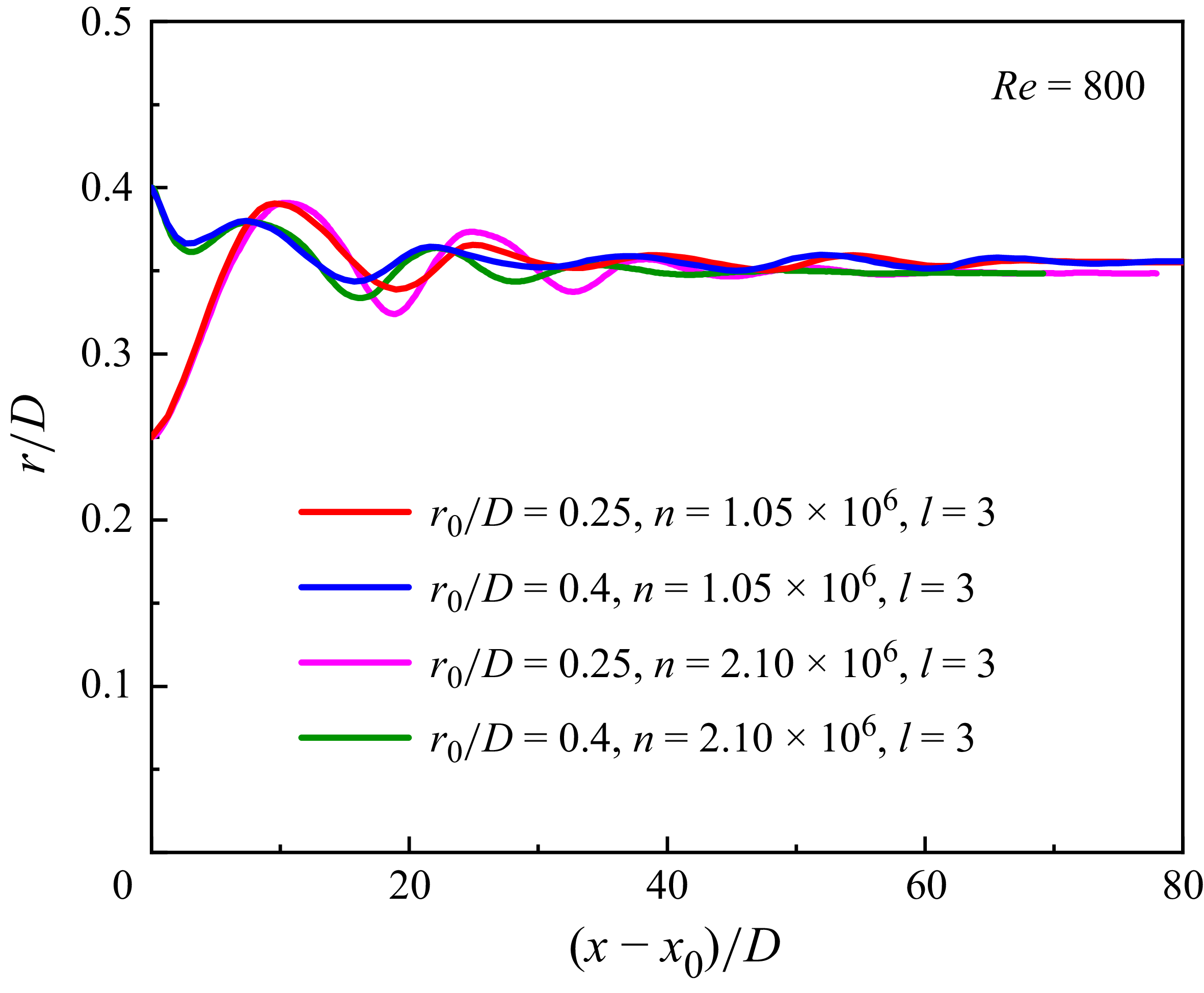
To investigate the potential role of mesh resolution on the occurrence of two equilibrium points, we have performed additional simulations at two initial positions, namely
 $r_0/D = 0.25$
and
 $0.4$
, for the case with
 $Re = 800$
and
 $d/D = 0.167$
using finer initial mesh elements. As can be seen from figure 19, the inertial migration behaviour and the equilibrium radial position remain almost unchanged with respect to the mesh structure applied, while no inner equilibrium position is observed.
Inertial migration of a neutrally buoyant sphere in circular Poiseuille flow for different initial mesh element numbers. Simulations were performed at
 $r_0/D = 0.25$
and
 $0.4$
for the case with
 $Re = 800$
and
 $d/D = 0.167$
.

Appendix C. Effect of initial position and initial conditions
We performed simulations to assess the influence of the initial position as well as of the initial translational and angular velocities of the particle.
Figure 20 shows the particle trajectories for various initial radial positions under different Reynolds numbers. As shown in figure 20, the behaviour of inertial migration, including the critical Reynolds number separating the neighbouring regimes, is essentially independent of the initial position
 $r_0$
. Of course, if the sphere is initially located at the equilibrium radial position
 $r^*$
, then a short initial transient occurs. This initial phenomenon arises because the sphere cannot immediately adapt to the flow field due to inertial effects.
Inertial migration of a neutrally buoyant sphere in circular Poiseuille flow for different initial radial positions at
 $Re = 200$
–
 $800$
. Simulations were performed using
 $d/D = 0.167$
and different values of the particle’s initial radial position
 $r_0$
, encompassing all situations
 $r_0 \lt r^*$
,
 $r_0 = r^*$
and
 $r_0 \gt r^*$
.

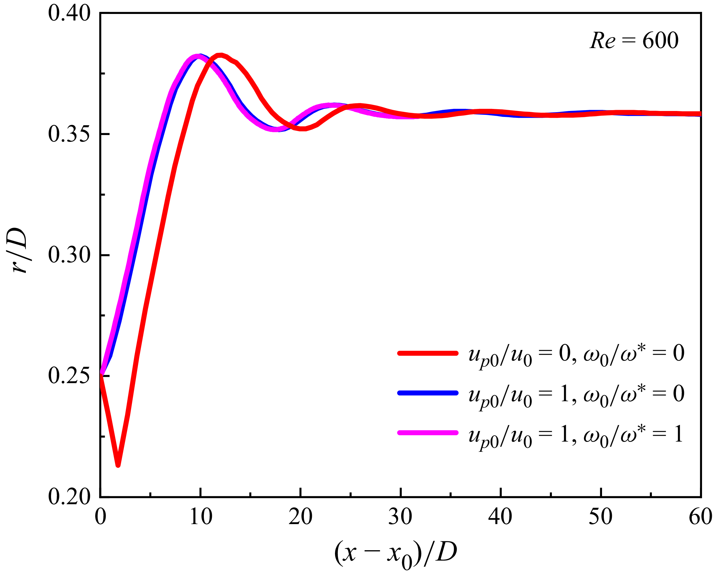
Figure 21 presents the particle trajectories for different initial velocities. As observed, the migration behaviour of the particle is nearly insensitive to its initial angular velocity as well. The particle’s initial translational velocity does not affect the final migration regime, although it has a small influence on the particle trajectory within the initial transient stage, during which the particle speed is adapting to the fluid velocity. Moreover, our simulations also reveal that, when
 $u_{{p0}}/u_0 = 0$
, the initial slip velocity between the fluid and the particle is large, generating a large slip-shear lift force, which in turn drives the particle towards the pipe’s central axis, initially.
Inertial migration of a neutrally buoyant sphere in circular Poiseuille flow for different initial velocities. Simulations were performed using
 $d/D = 0.167$
,
 $r_0/D = 0.25$
and
 $Re = 600$
. In the legend,
 $u_{{p0}}$
denotes the particle’s initial translational velocity,
 $u_0$
corresponds to the undisturbed fluid velocity at the centre of the particle at
 $t = 0$
,
 $\omega _0$
is the particle’s initial angular velocity and
 $\omega ^*$
denotes the particle’s final angular velocity at its equilibrium radial position.

Appendix D. Estimation of oscillation period
Using the results of our numerical simulations, we relate the period of the oscillations to the slope (stiffness) of the force profile around the equilibrium position and to the particle mass. According to the model of the damped harmonic oscillator, the particle’s radial displacement,
 $\xi = r {-} r^{*}$
, satisfies the equation
 \begin{equation} m_{p} \frac {\textrm{d}^{2}\xi }{\textrm{d}t_0^{2}} + \gamma \frac {\textrm{d}\xi }{\textrm{d}t_0} + k \xi = 0, \end{equation}
where
 $t_{{0}}$
is the oscillation time,
 $\gamma$
the damping coefficient and
 $k$
the slope (stiffness) of the force profile around the equilibrium position. Given the initial conditions
 $\xi = 0$
and
 $\xi ' = V_0$
at
 $t_{{0}} = 0$
, with
 $V_0$
denoting the radial migration velocity of the sphere as it first crosses the equilibrium radial position (
 $t_0 = 0$
), the solution of (D1) reads
 \begin{equation} \xi (t_0) = \frac {V_0}{\omega _{{d}}} \exp (-\zeta \omega _{{n}} t_0) \sin (\omega _{{d}} t_0), \end{equation}
where
 $\omega _{{d}}$
is the damped natural frequency,
 $\omega _{{n}}$
the natural frequency and
 $\zeta$
the damping ratio. These are given by the equations
 \begin{equation} \omega _{{d}} = \omega _{{n}} \sqrt {1 - \zeta ^2}, \quad \omega _{{n}} = \sqrt {\frac {k}{m_{p}}}, \quad \zeta = \frac {\gamma }{2 \sqrt {k m_{p}}}. \end{equation}
The period of the sphere’s oscillatory motion can thus be written as
 \begin{equation} T = \frac {2 \pi }{\omega _{{d}}} =2 \pi \sqrt {\frac {m_{p}}{k(1 - \zeta ^{2})}}. \end{equation}
In (D4), the stiffness
 $k$
is determined from the absolute value of the slope of the radial resultant force
 $F_r(\xi )$
at
 $\xi = 0$
, i.e. when the particle is at its equilibrium position and on the way towards the minimum radial position, within the first cycle of its oscillatory motion. Furthermore, the damping ratio
 $\zeta$
is evaluated as (Thomsen Reference Thomsen2021)
 \begin{equation} \zeta = \frac {\Delta }{\sqrt {4 \pi ^2 + \Delta ^2}}, \end{equation}
where
 $\Delta = \ln (A_1/A_2)$
is the logarithmic decrement, with
 $A_1$
and
 $A_2$
standing for the amplitudes in the first and second oscillation cycles, respectively.
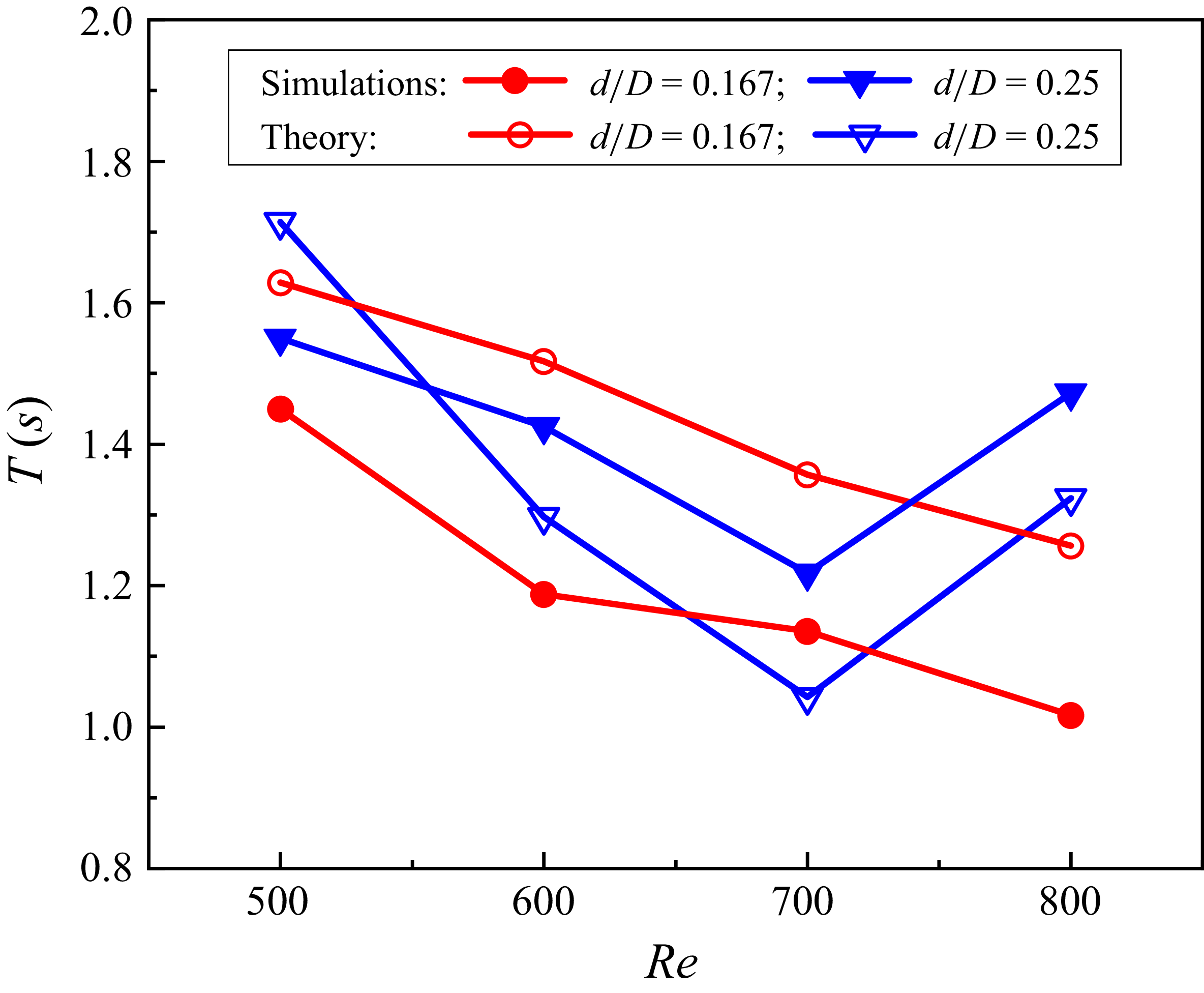
Figure 22 presents a comparison of the oscillation periods calculated theoretically using (D4) with those obtained from the numerical simulations for different values of
 ${\textit{Re}}$
and
 $d/D$
. As can be seen from figure 22, reasonable agreement between the values predicted from the theoretical model and those obtained from the numerical simulation is achieved.
Comparison of the oscillation periods calculated theoretically using (D4) with those obtained from numerical simulations at different
 ${\textit{Re}}$
and
 $d/D$
.

Appendix E. Final rotational velocity rescaled by local shear
We note that the local shear,
 $\tau$
, at the particle’s final equilibrium radial position in a circular Poiseuille flow is proportional to the fluid velocity gradient, following the expression
 \begin{equation} \tau \propto \left | \frac {\textrm{d}u}{\textrm{d}r} \right |= \frac {16\,\bar {u}\,r^{*}}{D^{2}}. \end{equation}
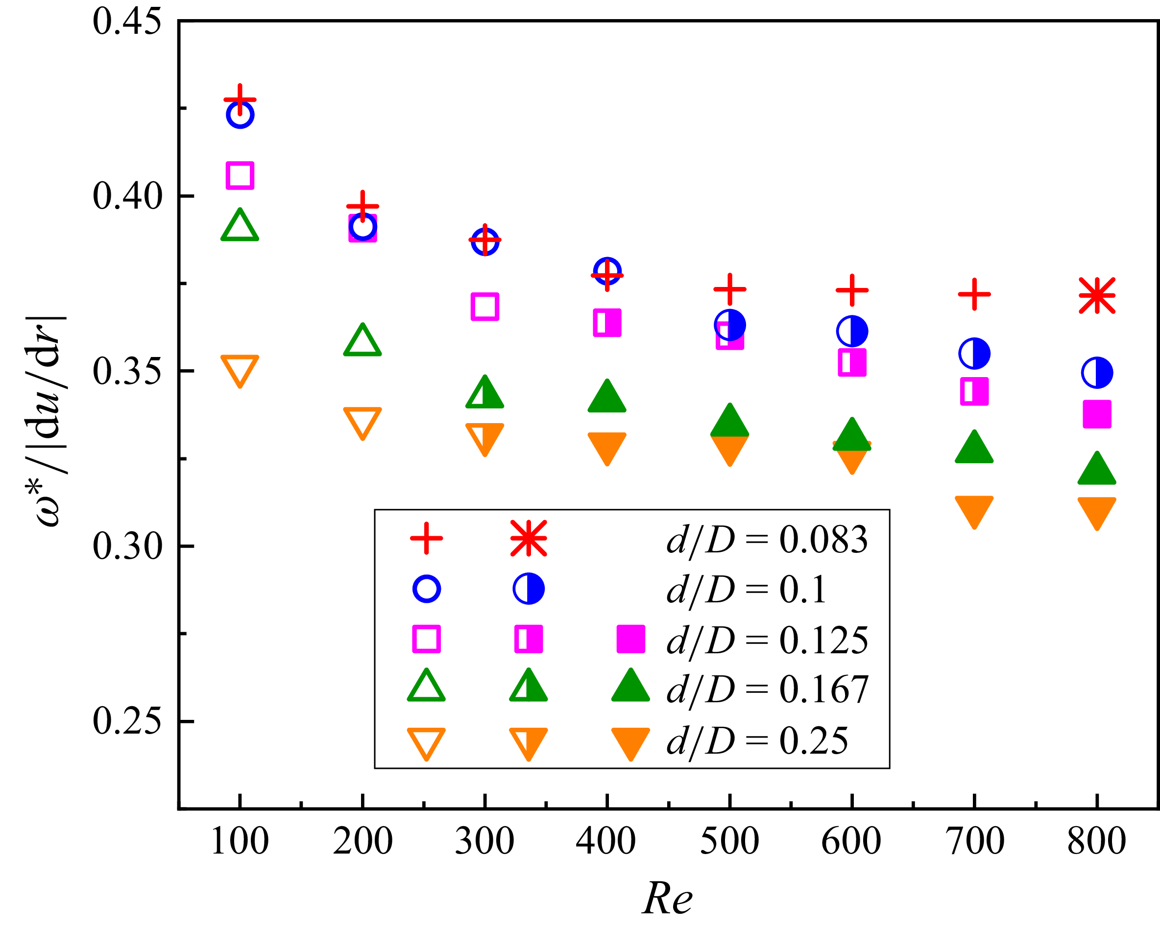
Figure 23 displays the final values of the sphere’s rotational velocity,
 $\omega ^{*}$
, rescaled by the velocity gradient
 $\left | \textrm{d}u / \textrm{d}r \right |$
at different values of
 ${\textit{Re}}$
and
 $d/D$
. As can be seen from figure 23, the variation of
 $\omega ^{*} / \left | \textrm{d}u / \textrm{d}r \right |$
with
 ${\textit{Re}}$
follows a similar trend across all values of
 $d/D$
; however, the respective magnitudes do not quantitatively agree over the entire range of
 ${\textit{Re}}$
and
 $d/D$
examined. As discussed by Bluemink et al. (Reference Bluemink, Lohse, Prosperetti and van Wijngaarden2008), for a non-inertial (
 $u_{0} d / \nu \approx 0$
, where
 $u_{0}$
is the undisturbed fluid velocity at the sphere centre), neutrally buoyant sphere in linear shear flow, the rotational velocity follows the relation
 $\omega ^{*} / \left | \textrm{d}u / \textrm{d}r \right | = 0.5$
. Our numerically obtained values of
 $\omega ^{*} / \left | \textrm{d}u / \textrm{d}r \right |$
are consistently smaller than 0.5 and exhibit a decreasing trend with increasing
 ${\textit{Re}}$
and
 $d/D$
. This behaviour indicates that inertial effects play an increasingly important role for the particle trajectory as the flow Reynolds number and the sphere-to-pipe diameter ratio increase.
Final values of the sphere’s rotational velocity,
 $\omega ^{*}$
, rescaled by the velocity gradient
 $| \textrm{d}u / \textrm{d}r |$
at different
 ${\textit{Re}}$
and
 $d/D$
. Crosses (
 $+$
) and open symbols denote the monotonic regime, asterisks (
 $\ast$
) and half-filled symbols the overshooting regime, and filled symbols the oscillatory regime.