Health and stature

A broad spectrum of health conditions are related to stature and skeletal remains, and stature reflects net nutrition among the living, while femur or long bone length reflects height and net nutrition among the dead (Fogel et al., Reference Fogel, Engerman, Trussell, Floud, Pope and Wimmer1978; Steckel & Rose, Reference Steckel and Rose2002; Stekel et al., 2019). Among early patterns found in stature studies was that average heights decreased during the earliest years of industrialization – patterns known as the early industrial growth puzzle and antebellum paradox (Komlos, Reference Komlos1987; Fogel, Reference Fogel, Engerman and Ballman1986, p. 454, Figure 9.1; Steckel et al., Reference Steckel, Clark Spencer, Roberts and Baten2018; Steckel, Reference Steckel and Komlos1994). Health and net nutritional conditions were also related to height variation. For example, anaemia is the lack of healthy red blood cells in the circulatory system, which leaves an individual tired and weak (Fogel, Reference Fogel1994, p. 370; Bollet & Brown, Reference Bollet, Brown and Kenneth2003, pp. 21–23), and anaemia in both modern and historical populations is a primary nutritional stress related to iron deficiency (Bothwell, Reference Bothwell1995; Papathanasiou et al., Reference Papathanasiou, Meinzer, Williams, Clark Spencer and Steckel2018). Anaemia is also related to haemoglobin and sickle-cell anaemia, and therefore race. Iron deficiency also affects the skeletal system through cribia orbitalis, which are the active lesions localized in the orbital roof. Porotic hyperostosis is the spongy or porous bone tissue located around the cranial vault and reflects poor nutrition (Walker, Reference Walker1986; Goodman & Martin, Reference Goodman, Martin, Steckel and Rose2002, p. 28; Steckel et al., Reference Steckel, Sciulli, Rose, Steckel and Rose2002, pp. 67–72; Walker et al, Reference Walker, Bathurst, Richman, Gjerdrum and Andrushko2009). Poor net nutrition is also related to osteoarthritis and degenerative joint disease, which are progressive age-related conditions with net nutrition that accounts for how adult stature decreases with age (Denko, Reference Denko and Kenneth2003, pp. 234–236; Adams & Dolan, Reference Adams and Dolan2005; Williams et al., Reference Williams, Meinzer, Clark Spencer and Steckel2019, p. 253). Oral conditions related to health are dental caries, anti-mortem tooth loss and linear enamel hypoplasia. Dental caries result because of poor oral hygiene but also from diets where carbohydrates are prominent and related to higher rates of dental caries (Ubelaker & Newson, Reference Ubelaker, Newson, Steckel and Rose2002, pp. 356–359; Goodman & Martin, Reference Goodman, Martin, Steckel and Rose2002, pp. 25–27; Bereczki et al., 2019, pp. 175–177). Ante mortem tooth loss also occurs when teeth are weakened by poor diets and tooth decay. Linear enamel hypoplasia is the failure of tooth enamel to develop correctly during formative years, is diet related and is a measure for poor net nutrition related to skeletal development and height (Goodman & Martin, Reference Goodman, Martin, Steckel and Rose2002; Berecaki et al., 2019).

Figure 1.

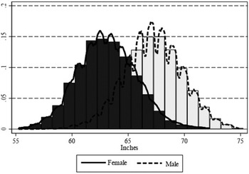
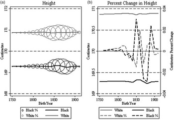
Late 18^th through early 20^th century women and men’s height. Source: Table 1.

Height as related to health is linked to mortality risk, and Waaler (Reference Waaler1984) and Fogel (Reference Fogel1994, pp. 378) illustrate that mortality risk is minimized for average male statures around 73 inches. Height is negatively related to all-source mortalities, which for women and men includes stroke and respiratory and coronary heart mortalities (Walker et al., Reference Walker, Shaper, Phillips and Cook1989; Palmer et al., Reference Palmer, Rosenberg and Shapiro1990; Yarnell et al., Reference Yarnell, Limb, Layzell and Baker1992; Leon et al., Reference Leon, Davey-Smith, Shipley and Strachan1995; Nwasokwa et al., Reference Nwasokwa, Weiss, Gladstone and Bodenheimer1997; Davey-Smith et al., Reference Davey-Smith, Hart, Upton, Hole, Gillis, Watt and Hawtorne2000, pp. 97–99; Song et al., Reference Song, Davey-Smith and Sung2003). Similar relationships exist between height, stomach and all-source cancers, indicating there is a link between mortality and height. Because stature reflects the cumulative net nutrition available to women from their formative years, understanding 18^th through early 20^th century gender-related stature variation and race throughout life sheds light on cumulative intra-family resource allocation. In addition, poor adolescent and childhood nutrition is related to later-life health outcomes (Barker, Reference Barker1992). For instance, shorter statures in early life are related to cognitive decline and dementia that may start during an adult’s early 50s (Sundet et al., Reference Sundet, Tambs, Harris, Mangus and Turjussen2005; Beauchamp et al., Reference Beachamp, Cesariri, Joehannesson, Lindquist and Apicella2011; Stewart et al., Reference Stewart, Hardy and Richards2015). In sum, stature is related to net nutrition, cumulative health and cognitive function in modern and historical populations.

Eighteenth through early 20^th century female and male stature data

Institutions in historical studies that randomly collected statures would have ideally collected height data under randomized controlled conditions. However, during early US economic development, these institutions were yet to develop. In the absence of historically randomized experiments, military and prison records are two sources used to evaluate historical height, and because of the number of male records that survive in military records, they are a primary source of data in stature studies. However, while plentiful, military records have various drawbacks, such as being drawn exclusively from men, and individuals in higher socioeconomic groups who were less vulnerable to nutritional variation (Sokoloff & Villaflor, Reference Sokoloff and Villaflor1982, pp. 456–458; Coclanis & Komlos, Reference Coclanis and Komlos1995, p. 93; Ellis, Reference Ellis2004, p. 27; Meinzer et al., Reference Meinzer, Steckel, Baten and Steckel2018, p. 239). Military records are also disproportionately drawn from individuals of European ancestry, and because women were not the focus of military physical requirements, military records offer no insight into 18^th through early 20^th century stature variation between genders. Fortunately, because of the size of the 18^th through early 20^th century US prison data set, a sufficient number of females exist to be compared with males.

Prison records are an alternative to military data, and there are advantages to using prison compared with military data. For example, prison resources include both females and males, and because the purpose of military records was violence, prison records are at an advantage to military records in representing the general population (Haines et al., Reference Haines, Haines and Steckel2000). Nevertheless, prison records are not beyond reproach, and incarceration reflects material and biological conditions among lower socioeconomic groups – that segment of society most vulnerable to biological change (Sokoloff & Vilaflor, Reference Sokoloff and Villaflor1982, pp. 456–458; Ellis, Reference Ellis2004, p. 27; Carson, Reference Carson2009c, Reference Carson2012; Bereczi et al., 2019, p. 190). Because inmates may have resorted to crime to survive, prison records may represent biological conditions among lower socioeconomic groups. Women also earned and accumulated less income and wealth than men and were unlikely to afford legal counsel at trial. Nevertheless, because prison records contain the greatest number of female statures, they are valuable resources when evaluating 18^th through 20^th century net nutritional conditions facing women and men.

Data to study 18^th through 20^th century female and male statures are part of an extensive effort to combine and collate historical heights using prison records (Carson, Reference Carson2008a, Reference Carson2009c). The prison sample used in this study was composed of 22 state prisons: Arizona, California’s Folsom and San Quinton, Colorado, Idaho, Illinois, Kansas, Kentucky, Maryland, Missouri, Mississippi, Montana, Nebraska, New Mexico, Ohio, Oregon, Pennsylvania’s East and West, Philadelphia, Tennessee, Texas and Washington prisons. There were 7682 females and 300,290 males, and women comprised about 2.5% of the US prison sample. In 1837 the Ohio State Prison was the first to construct an annex to house exclusively women, which was followed by New York in 1839, and the early perception of female prisoners was that they were threats to the moral foundations of society. During the earliest years of female incarceration, there were seldom female matrons, and physical and sexual abuse within prison was common (Rafter, Reference Rafter1985; Irwin, Reference Irwin1987).

Between the 1750s and early 1900s, prison enumerators recorded a broad set of personal characteristics, which included gender, birth period, complexion, nativity, decade received, age and occupation. Because they had legal implications in case an individual escaped and was later recaptured, physical characteristics were recorded in detail. Prison records were recorded at the time an individual was incarcerated; subsequently, prison records represent pre-incarceration conditions and not physical or occupational conditions within prisons. Physical characteristics also helped identify individuals within prisons.

Race was inferred from a complexion variable, and women and men of African descent were recorded as black, dark-black, chocolate and diverse shades of mulatto. Individuals of European ancestry were recorded as fair, white, light, medium and dark. These European complexions are supported further because individuals claiming European nativity in US prisons were also recorded with the same fair, white, light, medium and dark complexions. There were individuals of combined African and European ancestry who were recorded as mulattos. However, in the results that follow, women and men of combined African and European ancestry are referred to as ‘mixed-race’ (Carson, Reference Carson2015b). There was also a considerable share of individuals of Mexican ancestry in US prisons (Carson, Reference Carson2005, Reference Carson2007, Reference Carson2009a, Reference Carson2010b, Reference Carson2015a).

Prison enumerators recorded a broad set of occupations from which socioeconomic status was classified. Men from the clergy, government administrators and physicians were recorded as white-collar workers. Males who reported their occupations as butchers, carpenters and blacksmiths were recorded as skilled workers. Female white-collar and skilled workers were scarcer than males, and skilled women were typically in occupations that served the needs of other women (Burnette, Reference Burnette, Whaples and Parker2013; Carson, Reference Carson2018a). For example, skilled female workers included nurses and dress-makers. Farmers, ranchers and farm laborers were classified as farmers. Male labourers, cooks and miners were classified as unskilled workers. Female unskilled workers were domestic servants, labourers and cooks. A final category was included for individuals who recorded no decipherable or illegible occupation at the time of enumeration.

Over the 150 year span of this study, there are caveats when interpreting female and male occupations. Although occupations and job descriptions have changed considerably since the 19^th century, there was less 18^th and 19^th century job displacement because households were typically employed as unskilled workers or in agriculture (Steckel, Reference Steckel1983; Rosenbloom, Reference Rosenbloom2002, p. 88). Modern occupational distributions have also become less segregated along gender lines with technological change (Bleakley & Costa, Reference Bleakley and Costa2013, pp. 5–10). However, during the 18^th through early 20^th centuries, because of physical strength requirements, labour market opportunities differed considerably along gender lines (Goldin, Reference Goldin1990; Burnette, Reference Burnette, Whaples and Parker2013, p. 306; Marques et al., Reference Marques, Matos, Meinzer and Steckel2018, p. 158).

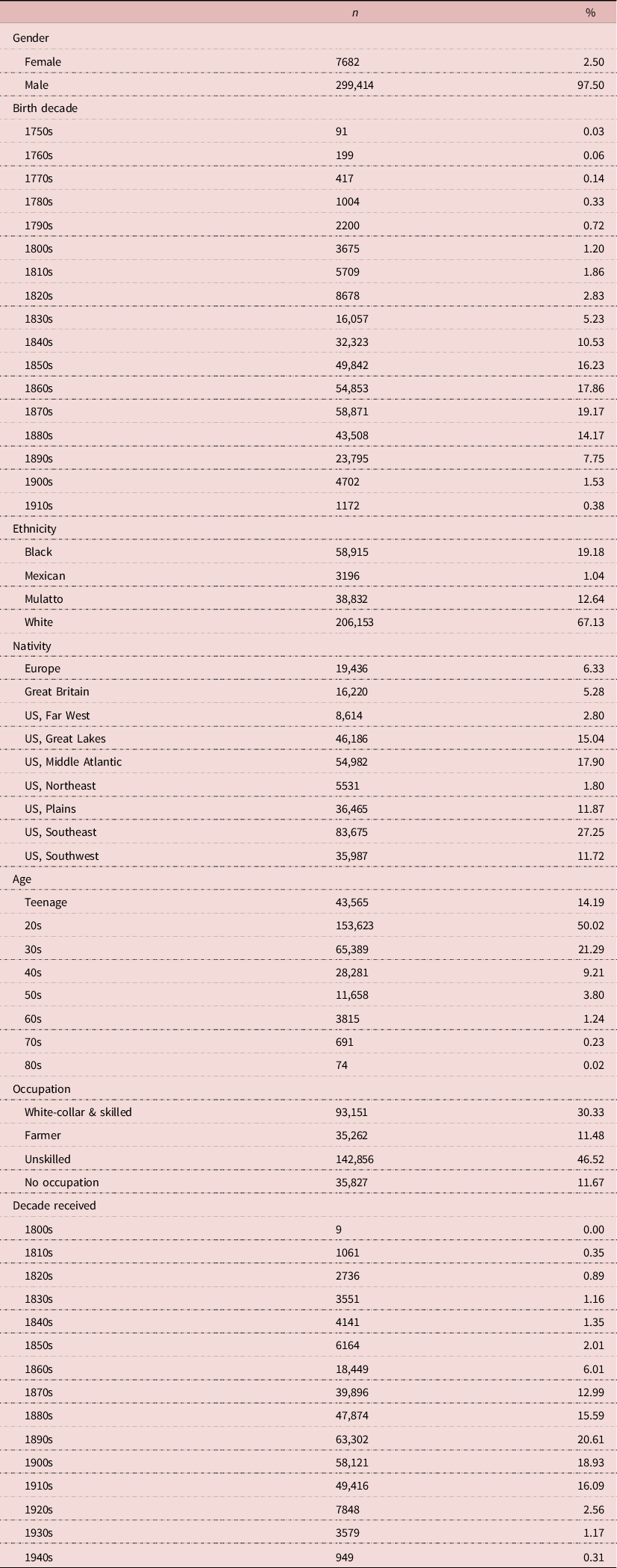
Whites were predictably the most common racial group; however, women and men of African descent were over-represented in US prisons relative to the general public (Table 1; Rafter, Reference Rafter1985; Steckel, 2000, Table 10.1, p. 435; Haines, Reference Haines, Haines and Steckel2000, Table 8.1, p. 306; Carson, Reference Carson2018a). Black over-representation in the prison sample may, in part, reflect vagrancy laws enacted during the years immediately after emancipation to prevent former slaves from exiting the labour force (Brands, Reference Brands2010, p. 156). The most common US nativity was the South. While there were substantial proportions native to the Great Lakes and Middle Atlantic, there were small proportions native to the Far West and Northeast. Individuals from Europe and Great Britain were sizeable cohorts in US prisons. Most individuals were born during the 1870s and observed in the 1890s. Whether it was from low income, little wealth and human capital or because of law enforcement targeting, younger individuals were more likely to be incarcerated in their 20s and 30s (Hirschi & Gottfredson, Reference Hirshchi and Gottfredson1983; Gottfredson & Hischi, Reference Gottfedson and Hirshchi1990; Carson, Reference Carson2009a, Reference Carson2018b; Baten et al., Reference Baten, Bierman, Luiten van Zanden and Foldvari2014; Baten & Steckel, Reference Baten, Steckel and Steckel2019). Low-skilled individuals were predictably the most likely to be incarcerated, while farmers were the least likely to be incarcerated. Subsequently, relative to workers in the general population, farmers were under-represented in the prison sample, while unskilled labourers were over-represented (Rosenbloom, Reference Rosenbloom2002, p. 88).

Table 1.

Female–male descriptive statistics

Sources: Arizona State Library, Archives and Public Records, 1700 W. Washington, Phoenix, AZ 85007; Colorado State Archives, 1313 Sherman Street, Room 120, Denver, CO 80203; Idaho State Archives, 2205 Old Penitentiary Road, Boise, Idaho 83712; Illinois State Archives, Margaret Cross Norton Building, Capital Complex, Springfield, IL 62756; Kentucky Department for Libraries and Archives, 300 Coffee Tree Road, Frankfort, KY 40602; Missouri State Archives, 600 West Main Street, Jefferson City, MO 65102; William F. Winter Archives and History Building, 200 North St., Jackson, MS 39201; Montana State Archives, 225 North Roberts, Helena, MT, 59620; Nebraska State Historical Society, 1500 R Street, Lincoln, Nebraska, 68501; New Mexico State Records and Archives, 1205 Camino Carlos Rey, Santa Fe, NM 87507Oregon State Archives, 800 Summer Street, Salem, OR 97310; Pennsylvania Historical and Museum Commission, 350 North Street, Harrisburg, PA 17120; Philadelphia City Archives, 3101 Market Street, Philadelphia, PA 19104; Tennessee State Library and Archives, 403 7^th Avenue North, Nashville, TN 37243; Texas State Library and Archives Commission, 1201 Brazos St., Austin TX 78701; Utah State Archives, 346 South Rio Grande Street, Salt Lake City, UT 84101; Washington State Archives, 1129 Washington Street Southeast, Olympia, WA 98504.

Between 1803 and 1946, female average stature was 160.10 cm, and male average stature was 170.80 cm, indicating males were over 10 cm taller than females (Figure 1; Gray & Wolfe, Reference Gray and Wolfe1980; Frayer & Wolpoff, Reference Frayer and Wolpoff1985). However, women’s stature standard deviation was greater than men: 7.11 to 6.84 cm. Female and male height distributions were also symmetric, indicating they were not affected by a truncation bias present in military samples (Sokoloff & Vilaflour, Reference Sokoloff and Villaflor1982, p. 456; Komlos & Kim, Reference Komlos and Kim1990).

Stature Coefficient of Variations and Gini Coefficients were used to illustrate cumulative net nutrition inequality (Morodi & Baten, Reference Moradi and Baten2005). To the extent that stature inequality represents material inequality, the male stature Gini Coefficient was 0.0223, and the female stature Gini Coefficient was 0.0244; the male stature Coefficient of Variation was 0.04006, and the female Coefficient of Variation was 0.04438; however, statures are genetically determined and are less responsive than other measures for inequality and are interpreted with caution. Subsequently, males were taller than females, whites were taller than blacks and stature inequality between females and males was similar.

Eighteenth through early 20^th century female and male statures by characteristics

Women and men’s 18^th through 20^th century statures are now regressed on demographic characteristics, complexion, age, nativity, birth decade and socioeconomic status.

\[\begin{gathered} Centimetre{s_i} = \;\alpha + {\beta _f}Femal{e_i} + \sum\limits_{c = 1}^3 {{\beta _c}} Complexio{n_i} + \sum\limits_{a = 1}^{15} {{\beta _a}Ag{e_i}} + \sum\limits_{n = 1}^8 {{\beta _n}Nativit{y_i}} \\ + \sum\limits_{t = 1750}^{1910} {{\beta _t}BirthYea{r_i}} {\text{ }} + \sum\limits_{l = 1}^3 {{\beta _l}Occupatio{n_i}} + {\varepsilon _i} \\ \end{gathered} \]

A binary female gender variable is included to account for the female–male stature difference (Gray & Wolfe, Reference Gray and Wolfe1980; Frayer & Wolpoff, Reference Frayer and Wolpoff1985; Floud et al., Reference Floud, Fogel, Harris and Sok Chul2011, p. 299). Black, mixed-race and Mexican race dummy variables are included to account for how stature and net nutrition vary by complexion and race (Steckel, Reference Steckel1979). Annual youth age dummy variables are included to account for female and male adolescent stature growth. Adult decade age dummy variables are included to account for how statures varied in older ages (Carson, Reference Carson2015b; Williams et al., Reference Williams, Meinzer, Clark Spencer and Steckel2019, p. 253; Goodman & Martin, Reference Goodman, Martin, Steckel and Rose2002, p. 44). There are two ways net nutrition is measured over time. Measured by birth year, biological measures reflect how individuals in the same birth cohort experience similar net nutritional conditions throughout life. Measured by current period, stature reflects how various groups experience the same biological conditions for the same period of measurement (Carson, Reference Carson2019, p. 32). Because stature growth had mostly ceased for women and men in their early 20s, statures are measured by birth year. Occupations reflect socioeconomic status, and five occupation variables are included: white-collar, skilled, farmers, unskilled and workers without occupations.

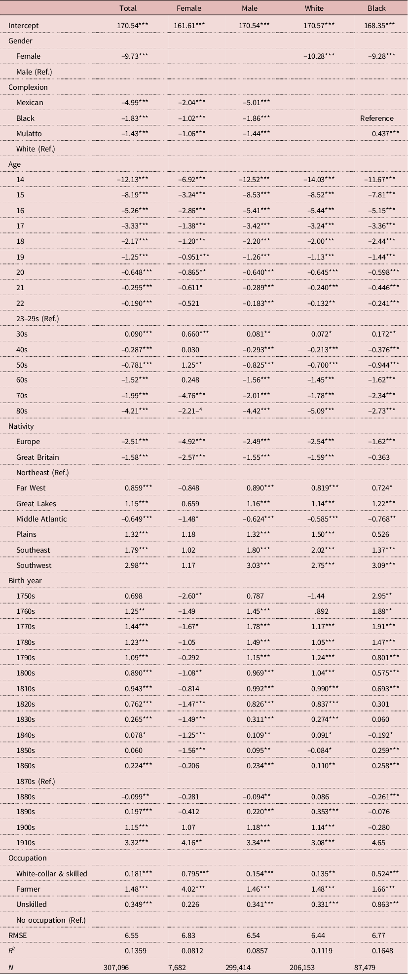
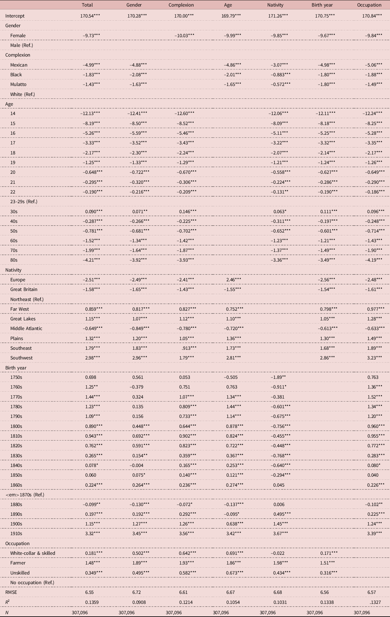
Table 2’s Model 1, Column 2, includes both female and male statures. Model 2, Column 3, includes only female statures, while Model 3 includes only male statures. To compare how net nutritional conditions varied throughout life by race, Models 4 and 5, Columns 4 and 5, include only individuals of European and African ancestry.

Table 2.

Female–male stature regressions, 1750–1820

Source: Table 1.

***p < 0.01; **p < 0.05; *p < 0.10.

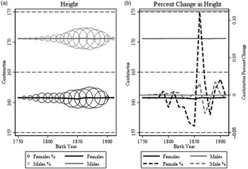
Three paths of inquiry are considered when comparing 18^th through 20^th century female and male stature variation. First, the antebellum paradox is the contradictory result that male statures ironically decreased during the 19^th century’s second and third quarters at the same time that wages and income monotonically increased (Lebergott, Reference Lebergott1984; Komlos, Reference Komlos1987; Bogart, Reference Bogart2009). However, this antebellum paradox and early growth puzzle have come under recent criticism that indicates stature variation is the result of selection bias (Bodenhorn et al., Reference Bodenhorn, Guinnane and Mroz2017). Nevertheless, selection was an important concern in early stature studies, and recent criticisms fail to account for an urbanization penalty across various studies and periods (Carson, Reference Carson2008b, Reference Carson2020; Komlos & A’Hearn, Reference Komlos and A’Hearn2019; Komlos, Reference Komlos2019). Little is known about how women and men’s statures in the US compared before the 19^th century, and to illustrate how net nutrition varied over time, stature trends in Figure 2 are presented with bubble figures, where circles represent proportional sample size (Carson, Reference Carson2011, Reference Carson2013). Eighteenth through 20^th century female and male statures remained approximately constant. Prior to the Civil War, female’s stature percentage decrease was greater than male’s and was larger at the end of the antebellum period. Male statures remained mostly constant throughout the 19^th through early 20^th centuries, and there was little convergence between female and male statures (Figure 2). Subsequently, males were taller than females, and female antebellum stature percentage changes were greater than male, indicating that women experienced greater net cumulative nutritional variation within the economy and the household. Collective stature variation is segregated into choice and non-choice characteristics, and stature variation over time is mostly a non-choice characteristic. The birth-year-restricted F-statistic is F(16, 307,049)=48.09 (p<0.001) indicating that birth years were collectively related for women and men, and birth period had a collective effect on stature variation.

Figure 2.

Male vs female stature by birth year. Source: Tables 1 and 2.

Figure 3.

White vs black male stature. Source: Tables 1 and 2.

Second, women and men classified as farmers had taller statures and superior net nutrition than workers in other occupations (Atack & Bateman, Reference Atack and Bateman1987, pp. 63–64). Moreover, the female farmer stature advantage was over twice that of males, whereas it was small and insignificant for women in other occupations. Two explanations account for taller agricultural worker statures relative to workers in other occupations. Agricultural workers may have been taller because rural agricultural lifestyles created greater access to diets rich in complex carbohydrates and animal proteins, which were associated with low disease burdens because they were in sparsely populated regions where disease was less likely spread (Carson, Reference Carson2010b, Reference Carson2020). Alternatively, farmers and agricultural workers were taller because agricultural occupations required greater strength and size to bear physical routines where size and strength were required (Margo & Steckel, Reference Margo, Steckel, Fogel and Engerman1992, p. 518; Steckel & Haurin, Reference Steckel, Haurin and Komlos1994, p. 122). Because women and men in rural agricultural areas were in close proximity to nutrition rich in animal proteins, farmers and agricultural workers were taller than workers in other occupations, indicating there were biological benefits to both female and male agricultural workers – taller female agricultural workers because there were positive cumulative net nutritional benefits that accrued to agricultural occupations related to rural agricultural lifestyles.

White-collar and skilled workers had taller statures than workers with no listed occupation, and the effect of female white-collar and skilled worker’s stature advantage was over five times the male white-collar and skilled advantage. However, unskilled female statures were about the same as women with no occupation, while the male unskilled effect was significant and greater than the male white-collar and skilled stature advantage. The black male white-collar and skilled occupational effect was nearly four times the size as the white male white-collar and skilled effect. The black unskilled stature effect was over twice the magnitude of the white unskilled stature effect. Women and men’s statures were collectively related to socioeconomic status, and the occupation-restricted F-statistic was F(3, 307,479)=385.89, indicating there was a collective effect between stature and socioeconomic status.

Third, height and net nutrition varied by race, and Steckel (Reference Steckel1979) was the first to find that individuals with fairer complexions were taller than individuals with darker complexions. Bodenhorn (Reference Bodenhorn2002) attributed the stature difference to 19^th century social preferences that disproportionately favoured individuals with fairer complexions. However, if whites were taller than blacks because of social preferences, whites should have had greater BMIs and heavier weights than workers with darker complexions. However, the opposite is true, and individuals with darker complexions consistently had higher BMIs and heavier weights (Carson, 2009, Reference Carson2012, 2015). Various explanations clarify why individuals with fairer complexions had higher BMIs and weight than whites. For example, with emancipation, freed slaves devoted a higher share of household wealth compared with whites to the acquisition of food (Higgs, Reference Higgs1977, p. 105); however, black diets included more fat-back pork. Statures were also collectively related to race, and the race-restricted F-statistic was F(3, 307,049) (p<0.001).

Other patterns are consistent with expectations. Net nutrition varied with respect to macro-nutrients, which reflect regional crop variation and animal husbandry (Carson, Reference Carson2020). The Northeast and Middle Atlantic were agriculturally productive in dairy but lagged behind other regions in corn, wheat, pork and beef production (Hilliard, Reference Hilliard1972, pp. 135, 156, 166, 94 and 114; Atack & Bateman, Reference Atack and Bateman1987; Brands, Reference Brands2010, p. 202; Carson, Reference Carson2020). Statures and net nutrition similarly varied regionally by gender, and whites from the Plains and South were taller than blacks. There was little female regional stature variation. Statures were collectively related to nativity, and the nativity restricted F-statistic was F(8, 307,049) = 1,414.07, indicating that women and men’s statures were collectively related to nativity.

Sensitivity analysis and collective marginal effects

Female and male statures are sensitive to choice and non-choice characteristics (Table 3). For example, occupations and residence are two characteristics over which individuals exercise considerable control, while gender, race and age are characteristics over which individuals have no control. Multiple restriction F-tests assess the statistical significance of a restricted set of variables, and observable gender, race, age, demographic and socioeconomic variables were collectively related to 18^th through 20^th century statures. F-Statistics do not, however, provide the magnitude for the collective restricted cohorts (Miller, Reference Miller2005, pp. 37–38). The relative importance of each collective group is the change in the sum-of-squares regression when a restricted set of variables is restricted to illustrate the relative magnitude of a characteristics effect (Miller, Reference Miller2005, pp. 37–38). The terms SSR_ur and SSR_r are unrestricted and restricted sum-of-squares regression; SSE_ur and SSE_r are unrestricted and restricted sum of squared errors; and $R_r^2$ and $R_{ur}^2$ are restricted and unrestricted coefficients of determination.

$$\%\Delta {\rm{SSR}} ={ {\rm{SSR}_{\rm r}-\rm{SSR}_{{\rm{ur}}}}\over{\rm{SSR}_{\rm{u}}} }= {{\rm{SSE}_{{\rm{ur}}}-{\rm{SSE}}_{\rm{r}}}\over{\rm{SST-SSE}_{\rm{ur}}}} = {{R_{\rm{r}}^2-R_{\rm{ur}}^2}\over{R_{\rm{ur}}^2}} = \% \Delta {R^2}$$

Table 3.

Female–male stature sensitivity analysis by demographic characteristics, socioeconomic status and birth decade

Source: See Table 1.

Notes: ***p < 0.01; **p < 0.05; *p < 0.10.

The stature magnitude difference between choice and non-choice characteristics is calculated by comparing restricted and unrestricted percentage changes in R ². The R ² percentage reduction when gender is excluded had the greatest reduction of –33.19 per cent, followed by nativity at –24.14 per cent and age at –22.44 per cent. Race and complexion, while still considerable, had less of a collective effect with stature variation with a –10.67 per cent R ² reduction. Socioeconomic status and birth year had the smallest effects with per cent R ² reductions of –2.36 and –1.55 per cent, indicating there were small collective stature effects for socioeconomic status and birth. In sum, after controlling for demographic and socioeconomic effects, gender has the greatest collective explanatory effect with stature variation, followed by age, nativity, race, socioeconomic status and birth year.

Accounting for the differences between structural and compositional effects

Female–male stature decompositions were used to assess how stature differences were attributable to returns to characteristics versus average characteristics. A Blinder–Oaxaca decomposition is a statistical technique used to partition the difference between two dependent variables into characteristic stature returns and average characteristic differences.

Gender

Let S _m and S _f be male and female statures; β _m and β _f and are structural sensitivity coefficients that reflect how male and female statures responded to changes in characteristics, whereas X _m and X _f are male and female average characteristic matrices. Because males are genetically taller than females due to genetics and sexual dimorphism, males are classified as the base structure (Gray & Wolfe, Reference Gray and Wolfe1980; Frayer & Wolpoff, Reference Frayer and Wolpoff1985; Floud et al., Reference Floud, Fogel, Harris and Sok Chul2011, p. 299; Carson Reference Carson, Komlos and Kelly2016):

(1) $$S_m = \alpha_m + \beta_m X_m $$

and

(2) $$S_f = \alpha_f +\beta_f X_f$$

The male–female stature gap is the difference between Equations (1) and (2):

(3) $$\Delta S = S_m - S_f = \alpha_m +\beta_m X_m - \alpha_f - \beta_f X_f $$

The Oaxaca decomposition is evaluated relative to a counterfactual. Equation (4) is male stature returns observed at female characteristics, while Equation (5) is female stature returns observed at average male characteristics:

(4) $$\beta_m X_f - \beta_m X_f =0 $$

and

(5) $$\beta_f X_m - \beta_f X_m =0 $$

Equation (6) is the male–female stature decomposition for male stature returns observed at female characteristics and is constructed by adding Equation (4) to Equation (3). Equation (7) is the male–female stature decomposition for female stature returns observed at male characteristics and constructed by adding Equation (5) to Equation (3).

(6) $$\Delta S=S_m - S_f =( \alpha_m - \alpha_f )+(\beta_m - \beta_f )X_f +\beta_m (X_m - X_f ) $$

(7) $$\Delta S=S_m - S_f =( \alpha_m - \alpha_f )+(\beta_m - \beta_f )X_f +\beta_m (X_m - X_f ) $$

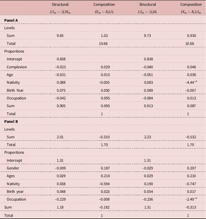
Average male stature was greater than that of females, and the greatest source of gender-based male stature advantage was in unobserved differences in the intercept, which includes differences in genetics, nutrition and income (Gray & Wolf, Reference Gray and Wolfe1980; Frayer & Wolpoff, Reference Frayer and Wolpoff1985). Nativity stature returns had the greatest explanatory effect across genders, followed by birth years. However, gender-based compositional effects by nativity were small, and there were large stature return differences by birth year, indicating gender-based nativity returns were greater for males than females.

Complexion

Statures were also decomposed by complexion. Because whites are, on average, taller than blacks, whites are assigned the base structure (Steckel, Reference Steckel1979; Carson, Reference Carson2009c).

(8) $$S_w = \alpha_w +\beta_w X_w $$

(9) $$S_b = \alpha_b +\beta_b X_b $$

The white–black stature gap is the difference between Equations (8) and (9):

(10) $$\Delta S=S_w - S_b = \alpha_w +\beta_w X_w - \alpha_b - \beta_b X_b $$

Equation (11) is white stature returns evaluated at black characteristics, and Equation (12) is black stature returns evaluated at average white characteristics:

(11) $$\beta_w X_b - \beta_w X_b =0 $$

(12) $$\beta_b X_w - \beta_b X_w =0 $$

Equation (13) is the white–black stature decomposition for white returns to characteristics observed at average black characteristics. Equation (14) is the white–black stature decomposition for black returns to characteristics observed at average black characteristics:

(13) $$\Delta S=S_w - S_b =( \alpha_w - \alpha_b )+(\beta_w - \beta_b )X_b +(X_w - X_b )\beta_w $$

(14) $$\Delta S=S_w - S_b =( \alpha_w - \alpha_b )+(\beta_w - \beta_b )X_w +(X_w - X_b )\beta_b $$

White statures were taller than black’s, and the greatest source of the race-based white stature advantage was in the unobserved intercept differences, which includes differences in genetics, nutrition and income (Table 4). Black socioeconomic structural returns were considerably greater than those of whites, with little difference in compositional returns, indicating gender-based socioeconomic returns were associated with large socioeconomic returns to black social status. Whites, on the other hand, had the greatest stature returns associated with birth year, nativity and age. Nevertheless, there were large white gender-based differences to compositional effects, indicating the white stature advantage by birth year, nativity and age was associated more with sample composition and were less causal.

Table 4.

Late 18^th through early 20^th century female–male stature decompositions

Source: Table 1 and Table 2.