





Policy Significance Statement
The Global Transnational Mobility Dataset 2.0, created as an outcome of this research, offers policymakers, development agencies, and public health authorities a resource to understand and respond to global mobility trends beyond conventional migration statistics. By incorporating diverse forms of transnational movement—and highlighting that conventional migration only captures less than 1% of global population movements—the dataset invites more nuanced migration policies, targeted remittance strategies, and sustainable tourism planning. Its long-term, global coverage supports climate policy design by revealing disparities in travel-related emissions between populations and informs epidemic preparedness through realistic mobility estimates. Furthermore, the dataset challenges existing globalization metrics by highlighting the human dimension of cross-border interaction. Insights from the dataset can help governments and international organizations craft more effective and equitable policies that reflect the full spectrum of global human mobility.
1. Introduction
Global mobility is one of the hallmarks of our age, representing the human dimension of globalization (Smith and Favell, Reference Smith and Favell2006; De Haas et al., Reference De Haas, Castles and Miller2020; Deutschmann, Reference Deutschmann2022; Recchi and Safi, Reference Recchi and Safi2024). This mobility is fed by migratory and non-migratory travel across countries. While migration is a major topic in public and academic discourse in most countries, non-migratory travel has only recently gained more attention. Conventionally, migrants (including asylum seekers and refugees) are defined as persons who change their country of residence for at least one year, while persons arriving in a country temporarily for non-residential purposes such as tourism, seasonal work, business travel, digital nomadism, or other reasons are classified as visitors (UNDESA, 1998, 2010, 2025).
Although this conventional categorization suggests a clear distinction between migrants and visitors, it is not obvious that non-migratory mobilities are entirely different from migration. For example, populations who repeatedly visit their international destinations—such as temporary workers, digital nomads, or transnational retirees—may not differ significantly from migrants in their life experiences and pathways—especially when compared to migrants near the one-year cut-off (i.e., the 12-month stay that qualifies as “migration” in the conventional definition). Additionally, despite the large volume of visitor mobility and its impact on destination societies, there is limited systematic information about the volume and direction of non-migratory global mobility flows. As a result, international mobility is almost exclusively discussed and studied in terms of migration.
To address this gap, this article presents estimates of global mobility flows between 243 countries and areas from 1995 to 2022 that combine both migratory and non-migratory forms of movement across borders. Our estimates aim to capture international mobility as represented in travel events serving a wide range of mobility goals, such as permanent settlement, seasonal migration, or those associated with mobile lifestyles. To achieve this, we synthesize three major sources of information about global mobility: tourism data from the UN World Tourism Organization, air passenger data from a private data provider, and migration data from estimates by Abel and Cohen (Reference Abel and Cohen2019, Reference Abel and Cohen2022a).
The Global Transnational Mobility Dataset 2.0 (GTMD2), created as an outcome of this research, is an update of Recchi et al.’s (Reference Recchi, Deutschmann and Vespe2019) GTMD, which estimated country-to-country human mobility between 2011 and 2016. Our GTMD2 considerably extends the annual coverage to 1995–2022 and refines the concepts and methods used in the previous version. This comprehensive dataset invites researchers and practitioners to widen their focus and direct their attention to the patterns, drivers, and consequences of those forms of international mobility that are otherwise made invisible by an exclusive focus on long-term resettlements only. We use the terms “international” and “transnational” interchangeably. In our reading, transnational refers to movements by non state actors that spans across national borders, as used in international relations, and thus being distinct from “international,” which refers to state actors (Nye and Keohane, 1971). In migration studies, “transnational” refers to movements of the same individuals across borders (Wimmer and Glick-Schiller, 2002), which does not apply in this work.
We demonstrate the usefulness of the new dataset by addressing three research questions.
-
1. How did total global mobility volumes develop between 1995 and 2022?
-
2. What is the relationship between migratory and non-migratory global mobility?
-
3. What are the dynamics in the global mobility network, and which are its major hubs?
Our estimates indicate that total global transnational mobility amounted to 5.29 billion trips in 1995, rising without major interruptions to 10.66 billion in 2019. Affected by the COVID-19 pandemic, mobility dropped to 4.77 billion in 2020 and recovered to 8.13 billion by 2022. In comparison, the world population increased from 5.75 billion in 1995 to 7.81 billion in 2019 (8.01 in 2022). With an average annual growth rate of 3.08% between 1995 and 2019, mobility has expanded faster than the global population (1.28% in the same period). On average, 56.7% of all border crossings are to European countries, the largest share by far, followed by Eastern and South-Eastern Asia at 10.9%. Oceania has the smallest share, with less than 1%.
International migration, defined as cross-border residence changes, constitutes only a small fraction of total border crossings. Central and Southern Asia has the highest share at 1.5%, followed by Oceania. In other regions, migration accounts for less than 1% of total mobility, with Europe having the lowest share at .12%. Overall, the share of migration in global mobility has decreased between 1995 and 2019.
While our estimates document a continued increase in international mobility, they also show that this increase is associated with intensified regional integration: four of five cross-border travels occur within the same world region, with an upward rather than downward trend. Although there are some “tectonic shifts” in the configuration of the global mobility network over time, such as the fusion of the Northern and Southern American clusters, or the eastward drift of the cluster around UAE, the network remains structured around eight or nine regional clusters continually.
The remainder of this article is structured as follows. In Section 2, we review existing resources on global mobility—both migratory and non-migratory—and discuss our GTMD2 in relation to them. In Section 3, we detail the conceptual framework behind our estimates of global travel volumes. In Section 4, we introduce the primary data sources on which we build the mobility estimates in the dataset. In Section 5, we lay out the details of our procedures to construct the dataset. In Section 6, we explore the dataset and describe general patterns of international mobility in response to the three research questions above. In Section 7, we discuss the empirical, theoretical, and practical implications of our new dataset and conclude.
2. Previous datasets on international mobility
As mentioned, the size and scope of international mobility are almost exclusively documented and discussed in relation to migration. The official sources are datasets curated by international organizations, such as the UN Trends in International Migrant Stocks database (TIMS), the World Bank’s Global Bilateral Migration database (GBM), or the OECD International Migration Database (IMDB), which draw on administrative data that their member states submit in regular intervals. These datasets differ in coverage and scope (see also Table 1). While TIMS covers all 233 UN countries and areas from 1990 to 2024, the IMDB covers only OECD countries starting in 1995. Yet, while the IMDB reports annual inflows of foreign-born population, TIMS only reports stocks of the foreign-born population in 5-year intervals. In contrast, the GBM reports migrant stocks from 1960 to 2018 in 10-year intervals (Özden et al., Reference Özden, Parsons, Schiff and Walmsley2011). Overall, the official reports point to a steady increase of migrants in the world from 2.3% in 1970 to 3.6% in 2020 (IOM, Reference McAuliffe and Oucho2024, Table 1).
Overview of global mobility datasets

Table 1. Long description
The table consists of four columns: Name, Mobility, Coverage, and Sources.
* G T M D 2: Migratory plus non-migratory mobility. Coverage from 1995 to 2022 across 243 countries with annual flows. Sources include U N tourism, flight data, and A and C migration estimates.
* G T M D 1 Recchi et al. 2019: Non-migratory mobility. Coverage from 2011 to 2016 across 196 countries with annual flows. Sources include U N tourism and flight data.
* Llano et al. 2023: Non-migratory mobility. Coverage from 1995 to 2018 across 74 countries with annual flows. Source is U N tourism.
* U N trends in international migrant stocks: Migration mobility. Coverage from 1990 to 2024 across 233 countries with 5-year stocks. Source is administrative data.
* O E C D international migration database I M D B: Migration mobility. Coverage from 1995 to 2022 for O E C D countries with annual flows. Source is administrative data.
* W B global bilateral migration database G B M: Migration mobility. Coverage from 1960 to 2018 across approximately 220 countries with 10-year stocks. Source is administrative data.
* Abel and Cohen 2019, 2022a, 2022b: Migration mobility. Coverage from 1990 to 2020 across 230 countries with 5-year flows. Source is T I M S.
* Standaert and Rayp 2022: Migration mobility. Coverage of annual flows. Sources include T I M S, I M D B, G B M, D E M I G, and I M F S C.
* Akbaritabar et al. 2024: Migration mobility. Coverage from 1998 to 2020 across 210 countries with annual flows. Source is online bibliometric data.
* Chi et al. 2025: Migration mobility. Coverage from 2019 to 2022 across 181 countries with monthly flows. Source is Facebook data.
Source: Authors’ own compilation.
Note. This table only includes datasets discussed in the main text.
In addition to these official sources, academic studies highlight previously unexplored aspects of international migration or use innovative ways to estimate migration flows. For example, Abel and Cohen (Reference Abel and Cohen2019, Reference Abel and Cohen2022a) use UN migrant stock data in a demographic accounting model to estimate outward, return, and transit migration flows and to distinguish sex-specific migration patterns; Standaert and Rayp (Reference Standaert and Rayp2022) use a Bayesian state-space model to combine multiple datasets on migrant stocks and flows into one estimate of global migration flows between 1960 and 2020; Chi et al. (Reference Chi, Abel, Johnston, Giraudy and Bailey2025) use digital records from Facebook users to estimate country-to-country migration flows; and Akbaritabar et al. (Reference Akbaritabar, Theile and Zagheni2024) use online bibliometric data to estimate international migration flows of scholars.
While the evidence shows that migration has increased, it is among the least common forms of international mobility. Non-migratory mobilities are much more prevalent, but only sparsely documented in large-scale datasets. For instance, the estimates by Recchi et al. (Reference Recchi, Deutschmann and Vespe2019) show that the volume of non-migratory mobility was more than 300 times larger than that of migration in 2016, meaning that international movements leading to long-term settlements accounted for only 0.3% of all annual mobility flows (ibid., p. 12). To illustrate this, on an international flight or train ride with 300+ passengers, only one will be a migrant; all others are visitors or returning visitors.
Recchi et al.’s (Reference Recchi, Deutschmann and Vespe2019) GTMD presents estimates of country-to-country human mobility between 2011 and 2016 that integrate global statistics on tourism and air passenger traffic. The innovation of their approach is combining tourism data from the UN World Tourism Organization (UNWTO) and air traffic data from Sabre, a private company providing market analyses to the travel industry. These sources had not been used jointly before. The idea behind merging both sources is that, in principle, administrative and transportation data yield the same volumes of travel between any two countries. This allows testing their relative contributions, correcting for limitations, and filling in missing data in either of the sources. To facilitate the merging, Recchi et al. (Reference Recchi, Deutschmann and Vespe2019) first construct a unified measure of tourism flows from the eight different tourist categories of the UNWTO data and, second, correct the Sabre air passenger volumes such that they approximate travel via all modes of transport. We follow similar steps but revise the specific procedures to reflect methodological improvements and formally include migration statistics as well.
A further contribution related to ours is the study by Llano et al. (Reference Llano, Pardo, Pérez-Balsalobre and Pérez2023) who estimate bilateral tourism flows among 74 countries from 1995 to 2018. Their main goal, which we share, is to harmonize the extremely heterogeneous information provided in the UNWTO tourism data. Thus, their study corresponds to the step in our dataset construction that prepares the tourism data for the merger with the air passenger data. In addition, Llano et al. (Reference Llano, Pardo, Pérez-Balsalobre and Pérez2023) aim to provide estimates of international and domestic tourism flows disaggregated by mode of transport. In contrast, we do not focus on the mode of transport, which is one of the factors limiting their sample to 74 countries. Moreover, they differentiate between overnight visitors (tourists) and the broader category visitors, which also include same-day visitors (excursionists), while we focus on visitors (overnight and same-day). A commonality between their paper and ours is the use of gravity models to harmonize the UNWTO data. While they follow conventions in the gravity of tourism literature, we adopt more recently developed methods in the trade and migration gravity literature.
Finally, an advantage of our data is that it not only covers more countries (243 vs. 74) but also extends to the period after 2018, which allows users of our data to evaluate the effect of the COVID-19 period travel restrictions imposed on large parts of the world population. We achieve a broader country coverage because we also integrate the air passenger data into our final estimates of non-migratory mobility flows.
Table 1 summarizes the characteristics of the other resources discussed in this review section.
3. Definitions and conceptual framework
3.1. Who are international travelers?
In this section, we define broad categories of international travelers. A traveler is a person who moves between different geographic locations for any purpose and duration (UNDESA, 2010, para. 2.4). Hence, if the locations are separated by international borders, the person moving between them is an international traveler. Conceptually, we intend to treat all cross-border movements equally, eschewing the methodological nationalism implied in conventional definitions of migration. Since, however, we need to draw our data from official (i.e., state-centered) sources, we distinguish between two kinds of international travelers—visitors and migrants—depending on whether their border crossing also represents a change of country of usual residence. Recently, the United Nations have issued revised Recommendations on Statistics of International Migration and Temporary Mobility (UNDESA, 2025). This document proposes a conceptual differentiation between international migration and international temporal mobility, depending on meeting a duration of stay criterion (typically 12 months or longer). Our concepts of visitors and migrants align with their two types of mobility; the GTMD2.0 is therefore a first global measurement of total mobility, leveraging existing sources.
3.1.1. Visitors
As visitors, we understand all people who travel across international borders without changing their country of usual residence. These include both same-day and overnight visitors, whatever their reason for travel. Reasons may include holiday, leisure, and recreational; business and professional; visiting friends and relatives; education and training; health and medical care; religion and pilgrimage; shopping; transit; adventure, or any other subjective reason humans may attribute to their spatial mobility. This definition of visitors is similar but not entirely congruent with the one in the UN’s Recommendations for Tourism Statistics 2008 (UNDESA, 2010, para. 2.41 ff.). For example, in contrast to the UN, we would conceptually also include international commuters who live in one country but regularly travel across international borders to reach their workplace without changing their usual residence. Think of employees whose employer deploys them to work in a country other than their country of residence (so-called “posted workers”) or cross-border workers who commute daily or weekly across international borders to their workplace. The latter category of international travel is more common in free-movement areas, such as the European Union, where non-residents can participate in a member state’s labor market based on their EU citizenship rights. Cross-border commuting is less common—albeit not absent—in other world regions.
3.1.2. Migrants
As migrants, we understand all people who travel across international borders and change their place of usual residence by doing so. We sometimes refer to them as “residence changers” or “future settlers.” This definition is similar to the UN’s Recommendations on Statistics of International Migration (UNDESA, 1998), which additionally distinguish between long-term and short-term migrants. Yet, our approach differs from most conventional categorizations as we do not differentiate between people by their motive of residence change, which may include work, study, family reunification, and threats to their life and health at home. Hence, for us, this group of residence-changing international travelers would conceptually include all those commonly referred to as permanent migrants (i.e., those staying abroad for longer than 12 months), but also refugees, temporary labor migrants, seasonal workers, transnational retirees, and digital nomads, provided that their international destinations are at least one of the places they usually reside in.
Finally, let us define the notions of origin and destination country. We will adopt a country of residence perspective, as opposed to a country of birth or citizenship perspective, to determine the origin country of a traveler. This means that a mobile person’s current country of residence is their country of origin, as they are currently part of that country’s population. Yet, the origin country of a traveler is not necessarily the same as the origin of an individual trip. So, imagine an
$ i $
 -country resident traveling between countries
$ j $
 and
$ k $
 . While country
$ i $
 is their origin country, country
$ j $
 is the origin of their current trip. However, most available migration and refugee statistics report the number of immigrants and refugees based on a country of birth or citizenship perspective. This has to do with how countries conduct population censuses, which is the typical source for international migration statistics, where migrant stocks and flows are usually reported in terms of foreign-born residents or foreign-born arrivals (UNDESA International Migrant Stock, 2020; OECD International Migration Database, 2024).
3.2. The composition and measurement of international mobility flows
Methodologically, our work is based on the idea that there are two main approaches to measuring the number of international border crossings. The first relies on administrative data about arrivals collected by receiving countries according to the broad categories outlined above. The second relies on passenger volumes in all possible modes of cross-border transport. We use elements of both to generate our estimates and discuss them in turn.
3.2.1. Trips as measured by type of traveler
Most receiving countries classify incoming travelers according to the above categories and keep records of these arrivals. Thus, in principle, the number of incoming persons from the different registries could be added to compute the annual total of trips between countries.
One difficulty with this approach is that receiving countries register arriving persons at different places and store this information in different registries. Typically, there is not one single reception desk for check-in upon arrival in a country. For instance, tourist visitors may be registered through their accommodation; cross-border workers may only be registered through their work permits; immigrants are registered by the respective government agencies (further distinguishing asylum seekers, for instance), and so forth. This means, however, that if one wanted to add up all arrival categories, first, one would need data from all the different registers, and second, these registry data would have to be comparable between countries (i.e., countries should classify arrivals based on the same criteria). Yet, although the UN issues recommendations on how to count tourists and other visitors (UNDESA, 2010), immigrants (UNDESA, 1998), and refugees (EU and UN, 2018), there is heterogeneity in how member states implement these recommendations. In particular, there is quite some difference in how receiving countries classify temporary and circular migration (ILO, 2022).
Notwithstanding these practical considerations, in principle, arriving visitors and migrants could be summed up to yield the total number of trips between countries. We note that the persons traveling through the
$ ij $
 -corridor could be
$ i $
 -residents leaving their country of residence
$ i $
 , or
$ j $
 -country residents returning from
$ i $
 to their country of residence
$ j $
 , or
$ k $
 -country residents who transit through country
$ i $
 on their way to their destination
$ j $
 . Hence,

where
$ {out}_{i, ijt} $
 stands for outgoing trips carried out by
$ i $
 -country residents,
$ {return}_{j, ijt} $
 stands for return trips carried out by
$ j $
 -country residents, and
$ {transit}_{k, ijt} $
 stands for transit trips carried out by third-country
$ k $
 residents.
More specifically,
$ {out}_{ijt} $
 includes travelers from both broad categories introduced above:
$ i $
 -resident visitors on their way to country
$ j $
 and migrants who change their residence from country
$ i $
 to country
$ j $
 . In contrast, the return trips
$ {return}_{ijt} $
 only include
$ j $
 -resident visitors returning from their stay in country
$ i. $
 So-called “return migrants,” that is,
$ j $
 -born individuals who return from their current or temporary country of residence
$ i $
 to their country of birth, are not present in the return trips. This is because migrants are residents in their host country and, therefore, are counted in the outgoing trips of
$ i $
 -residents. While they are called “return migrants” from a country-of-birth perspective, they are simply migrants, that is, repeated residence changers, from a country-of-residence perspective. Finally, the transit trips,
$ {transit}_{ijt} $
 , include
$ k $
 -resident visitors and migrants who transit through country
$ i $
 on their way to the final destination of their current travel in country
$ j $
 . We will not consider this kind of travel in our dataset. Transiting travelers usually represent only technical border crossings, for example, layovers at international airports, involving next to no meaningful engagement with a country or society.
Given these considerations, in this article, we use the following decomposition to operationalize our estimate of total cross-border trips between all countries of the world:

Hence,
$ {trips}^A $
 measures the total volume of travel in each travel corridor between the 243 countries in our study. It corresponds to all the travel events in a corridor performed by anyone, including the trips by outgoing visitors, returning visitors, and outgoing migrants.
Incidentally, equipped with the above concepts, one could construct a second measure of international travel, which, in contrast to trips A , includes outgoing visitors and outgoing migrants but does not include returning visitors. This second measure would, thus, capture the travel events of origin-country residents in each corridor. This could be useful to study the international mobility propensities of a country’s population. However, we leave this for future research and focus on the total volume of international travel between countries in the remainder of this article.
3.2.2. Trips as measured through transport volumes
The second approach to measuring border crossings relies on the volumes of passengers in various modes of transport. Typical forms of transport include airplane, car, rail, and ship traffic, but in some border regions, crossings on foot, bike, etc., are also not entirely uncommon. So, if one had records on incoming passengers, one could simply add up their numbers across all modes of transport to arrive at the total volume of trips between two countries.

where
$ {air}_{ijt} $
 represents the volume of passengers crossing international borders between country
$ i $
 and country
$ j $
 by airplane;
$ {land}_{ijt} $
 those in cars, trains, and other land-based modes of transport; and
$ {water}_{ijt} $
 all those traveling in ships and other water-based vessels.
One feature of this approach is that it does not allow us to distinguish between the two categories of transnational travelers discussed above (e.g., visitors and migrants). Moreover, this approach does not allow for distinction between outgoing, return, or transit trips if the passenger’s records do not include the residence country of the traveling person.
3.3. Strategy to estimate transnational mobility
Our strategy to estimate total border crossings between countries relies on the idea that, in principle, the two measurements should record the same amount of border crossings. So, our procedure follows two main steps: first, we estimate
$ trip{s}^A $
 and
$ trip{s}^B $
 using three of the largest existing records of border crossings; second, we combine them into one coherent measure of transnational mobility. Figure 1 illustrates our workflow. Here, we briefly outline its main building blocks and discuss details in the following sections.
Outline of the two-step procedure for dataset assemblage. Note: The dataset assemblage uses as input data from (a) the UN World Tourism Organization (UNWTO), (b) Abel and Cohen (Reference Abel and Cohen2019), and (c) Sabre air passenger flows. The resulting Series 1 (without imputation) and Series 2 (with imputation) are shown at the bottom and make up the GTMD 2.0 dataset. Source: Authors’ own illustration.

Figure 1. Long description
The flowchart is divided into two horizontal sections labeled Step 1 and Step 2.
Step 1 involves three input streams:
1. Left column: U N W T O inbound tourism data 1995-2022 undergoes data cleaning, transformation of tourists to visitor flows, and accounting for returning visitors. This results in revised U N W T O visitors plus returning visitors.
2. Middle column: Guy Abel migration flow estimates 1990-2020 are transformed to annual flows, resulting in revised Abel migration flow estimates 1995-2019.
3. Right column: Sabre passenger volumes 2010-2022 undergo replacement of missings in low-volume corridors by zero and distance correction.
At the end of Step 1, the left and middle streams merge into a box labeled trips super A equals visitors plus returning visitors plus migrants. The right stream leads to a box labeled trips super B equals distance adjusted passenger volumes.
Step 2 processes these two variables based on availability:
- If only trips super A available, it flows directly to the final dataset.
- If only trips super B available, it flows directly to the final dataset.
- If trips super A and trips super B available, a logic box applies: if trips super A is greater than or equal to trips super B, use trips super A; if trips super A is less than trips super B, use trips super B.
The final output is the Global Transnational Mobility Dataset 2.0 (G T M D 2.0), containing two series:
- Series 1: No imputation of missing values in trips super A and trips super B; no backcasting of trips super B.
- Series 2: Imputed isolated, missing values in trips super A and trips super B using linear interpolation; backcast of trips super B using a parsimonious gravity model.
Our three data sources are:
-
1. Inbound tourism, 243 origin and 211 destination countries, 1995–2022, UN Tourism Data, World Tourism Organization (UNWTO).
-
2. Migration flow estimates, 230 origin and destination countries, 1990–2020, Guy Abel.
-
3. Air passenger volumes, 254 origin and destination countries, 2010–2023, Market Intelligence Data, Sabre.
We limit our timeframe to the 1995–2022 period, for which we maximize data availability from the three sources. To unlock on the full potential of the Sabre data, we back-cast its information on a yearly basis to cover the 1995–2009 period. In later sections, we provide details and documentation on the robustness of this operation.
It should be noted that while these three datasets cover many forms of international travel, there are notable limitations. For instance, the UNWTO data do not cover commuting cross-border workers, while the Sabre data do not include land and sea travel. We will describe the methods we undertake to remedy some of these limitations (e.g., distance correction of the air passenger data) in the following and further discuss which mobilities are covered by the data when we introduce the data records in detail (Section 4).
Step 1 of our pipeline to assemble the dataset consists in estimating the constructs
$ trip{s}^A $
 and
$ trip{s}^B $
 . This involves revising the three data records such that they match our grid of origin–destination–year cells for all existing countries since 1995. Moreover, in the UNWTO data, which are reported in different tourism categories (e.g., arrivals at national borders, arrivals in hotels, and arrivals by non-nationals vs non-residents), we generate a unified metric of “non-resident visitors arriving at national borders.” Also, we add the same volume of visitors traveling in the
$ ij $
 -direction to those traveling in the
$ ji $
 -direction to approximate returning visitors. In the migration data, which is reported in 5-year intervals, we compute annual migrant flows by dividing by five. Finally, we add visitors, returning visitors, and migrant flows to obtain an estimate of
$ trip{s}^A $
 .
Then, to estimate
$ trip{s}^B $
 , we generate distance-adjusted air passenger volumes. The reasoning is that passenger volumes on airplanes will closely approximate the number of travelers between countries the farther apart they are; the closer these countries are, the more travelers will use other modes of transport. So, using the cases in which visitor data and air passenger data are available, we regress visitors on passengers and distance (and other accessory geographical information, such as the existence of land borders between countries), and use the coefficients to adjust the air passenger volumes to represent all modes of transport in corridors that are not only accessible by plane. This “distance” adjustment yields
$ trip{s}^B $
 .
In our second step, we combine
$ trip{s}^A $
 and
$ trip{s}^B $
 to create our dataset of global mobility flow estimates. We assume that, in principle, the two ways of measuring the number of international border crossings yield the same amount of border crossings. Therefore, we use the equality

to validate our
$ trip{s}^A $
 and
$ trip{s}^B $
 estimates, as well as to fill in values whenever
$ trip{s}^A $
 are missing. Based on Series 1 of our estimates, in some cases, we only have
$ trip{s}^A $
 (12%), in others only
$ trip{s}^B $
 (73%), and in the rest, we have both (15%). In cases we have only one of the two, we use this as an estimate of global transnational mobility. If we have both, we pick the record that returns the higher total volume in a corridor, assuming both will underestimate actual mobility flows (mostly because our data by default do not include irregular mobility and underestimate flows by cross-border workers). This maximizes the total amount of country-to-country estimates of human transnational mobility. We will provide statistics on which percentage comes from which source later on (Table 4).
4. Data records
We now introduce the data records we use to operationalize the conceptual constructs from the previous section. Note that the groups of migrants and visitors recorded by the administrative data sources do not fully align with our constructs. In this respect, we acknowledge a tension between our conceptual framework, which aims to move beyond rigid categorical distinctions, and the empirical implementation, which relies on data sources that are anchored in conventional definitions. However, as there are no other global mobility data records than the ones introduced below, we are bound by their current limitations. We will highlight differences between them and our definitions accordingly.
4.1. Visitor flows
To represent bilateral flows of non-resident visitors, we use data from the UNWTO’s Tourism Data in Excel Format—Data from 1995 onwards (UNWTO, 2024). More specifically, we use the data on Inbound Tourism, which reports tourist arrivals in destination countries annually between 1995 and 2002. The data record is a collection of 219 Excel files, each corresponding to one destination country. Among other indicators, these destination country-specific files contain the annual volume of arrivals by origin country, which we use as the bilateral visitor flows in Equation (2).
Arrivals represent the flow of international visitors to the reference country, where each arrival represents one inbound tourism trip. When a person visits multiple countries within a single trip, the arrival in each country is documented separately; hence, within a given accounting period, the number of arrivals may exceed the number of unique travelers; for example, if a person visits the same country multiple times in a year.
In this data record, inbound visitors refer to overnight and same-day foreign visitors who travel for specific reasons, such as holidays, business, visits to friends and relatives, etc., as specified in the classification of inbound visitors according to the UN’s International Recommendations for Tourism Statistics 2008 (UNDESA, 2010) (see Figure 2). Other categories of travelers—such as border, seasonal, and short-term workers—are excluded, as they do not fit the definition of visitors. Thus, the UN Tourism Data does not completely match our definition of visitors in Section 3.1, which is much broader and includes, for example, commuting workers who operate in a foreign country without this country becoming their usual residence. It is not detectable from the reported figures to which degree seasonal workers and other short-term workers are excluded from the UNWTO visitor data. For example, in countries that count visitors through records of people staying in hotels and similar establishments (e.g., many European countries), they might be captured by the UNWTO visitor data, at least to some proportion. Yet, as suitable data on short-term cross-border workers are notoriously difficult to obtain (ILO, 2022; OECD, 2019), we do with the UN Tourism Data and contend that our estimates will at least represent a lower bound of international border crossings.
Classification scheme for inbound travel data records. Note: Categories on the right-hand side are excluded from the inbound visitor statistics used in this study, which are broadly categorized into tourists and visitors. Reporting countries may classify visitors by nationality and/or country of residence. Spelling inconsistencies reflect the original source. Source: International Recommendations for Tourism Statistics 2008 (UNDESA, 2010).

Figure 2. Long description
A central vertical column begins with Other inbound travellers at the top, which connects down to Inbound travellers, then to Inbound visitors.
From Inbound visitors, the chart branches into two sub-categories: Tourists (Overnight visitors) on the left and Same-day visitors (Excursionists) on the right. Below these, the chart identifies residency classifications: Nationals residing abroad and Other non-residents (foreigners).
A horizontal line connects the central Inbound visitors section to a vertical list on the far left titled Main purpose of tourism trips. This list includes: Business and proffesional; Holiday, leisure and recreation; Visiting friends and relatives; Education and training; Health and medical care; Religion / pilgrimages; Shopping; Transit; and Other.
A line from the top box, Other inbound travellers, connects to a vertical list on the right representing excluded categories: Border workers; Seasonal workers; Other short-term workers; Long-term workers; Nomads and refugees; Transit passengers not entering the economic and legal territory; Crews on public modes of transport; Persons entering the country to establish there their country of residence; long-term students and patients and their family joining them; and Other travellers deemed not to enter the economic territory, which includes Diplomats, consular staff, military personnell and their dependants, and Armed forces on maneuver.
Finally, the reference countries in the UN Tourism Data record arrivals differently: some through border surveys, some through immigration offices, and some through accommodation surveys. Moreover, some countries count only overnight visitors but not same-day excursionists, and some define foreigners by nationality rather than residence. Overall, this results in eight arrival categories reported in the source data (see Table 2). As the visitor flow volumes cannot be compared across categories, we convert the arrival categories into one statistic, thus creating a unified measure of inbound visitors. Details are described in Section 5.2.
UNWTO arrival categories

Table 2. Long description
The table consists of three columns: code, label, and description.
* Row 1: Code 112, Label T F R, Description: Arrivals of non-resident tourists at national borders, by country of residence.
* Row 2: Code 111, Label T F N, Description: Arrivals of non-resident tourists at national borders, by nationality.
* Row 3: Code 122, Label V F R, Description: Arrivals of non-resident visitors at national borders, by country of residence.
* Row 4: Code 121, Label V F N, Description: Arrivals of non-resident visitors at national borders, by nationality.
* Row 5: Code 1912, Label T H S R, Description: Arrivals of non-resident tourists in hotels and similar establishments, by country of residence.
* Row 6: Code 1911, Label T H S N, Description: Arrivals of non-resident tourists in hotels and similar establishments, by nationality.
* Row 7: Code 712, Label T C E R, Description: Arrivals of non-resident tourists in all types of accommodation establishments, by country of residence.
* Row 8: Code 711, Label T C E N, Description: Arrivals of non-resident tourists in all types of accommodation establishments, by nationality.
Source: The numerical code is from the UNWTO inbound data files; label and description are taken from World Tourism Organization (2023) Methodological Notes to the Tourism Statistics Database, page 213.
Note: Reporting countries vary in how they define and count visitors, depending on their chosen statistical definitions and methods. This table lists the relevant UNWTO statistics codes, labels, and descriptions in full.
4.2. Migrant flows
To represent bilateral migration flows, that is, number of residence changes, we use data from Abel and Cohen’s Bilateral international migration flow estimates for 200 countries (Abel and Cohen, Reference Abel and Cohen2019, Reference Abel and Cohen2022b, Version 7 (October 2024)). This data record provides estimates of bilateral migration flows between 230 countries in six 5-year periods (1990–95, 1995–2000, …, and 2015–2020). To obtain annual data, we divide the 5-year flows by five and distribute them over the respective years, weighted by the population size in the origin country. This means that we end up with annual migration flows from 1990 to 2019.
We use these estimates rather than actual migrant flow counts, such as the OECD International Migration Database, because there is simply no dataset of international migrant flows with the country coverage appropriate for our project (cf. Table 1). Many countries do not publish data on bilateral migration flows and the countries that collect such data use differing criteria for defining migrants, preventing detailed cross-country comparisons.
To address these problems, the estimates in Abel and Cohen’s database are based on bilateral migrant stocks from the UN’s International Migrant Stock dataset (UNDESA, 2020). Migrant stock data measure the number of migrants living in each country at a given time by country of birth. Such measurements are reported regularly by all UN countries and are much easier to collect than flows, as only questions about place of birth need to be asked in a country’s census, population registers, or administrative data collection systems. The migrant stocks are adjusted to include refugee populations (UNDESA, 2020, p. 4 f.).
“Demographic accounting,” the estimation method used by Abel and Cohen (Abel, Reference Abel2013; Abel and Cohen, Reference Abel and Cohen2019; see also Azose and Raftery, Reference Azose and Raftery2019), transforms the birthplace-specific migrant stock data into flows between residence countries. This method ensures that migrant flows in each corridor include out-migration as well as return- and transit-migration. In our setting of residence-changing mobility, each out-, return, and transit-migrant counts as one border crossing. While these estimates capture migrants as residence-changers and, in principle, correspond to the definition of migrants we use in this article, the underlying migrant stocks are based on the conventional “longer than 12 months” definition of migrants. Hence, individuals who may reside in more than one country per year are not captured by these. Furthermore, we acknowledge that the Abel and Cohen estimates are only as good as the underlying stock data, which implies that if the stock data grossly underestimate migrant populations, for instance, in low- and middle-income countries, the Abel and Cohen estimates will do so too. However, their data represent the most complete record of migration flow data for the entire world, particularly because other datasets do not report on South–South migration at all (cf. Table 1).
As will become apparent later, the total number of migrants represents only a fraction of total border crossings. We like to emphasize that this is not an artefact of our choice of migration estimates. In fact, Abel and Cohen’s migration flow estimates yield the highest total annual flows compared to other migration estimates and are, on average, higher than actual, counted migration flows (Abel and Cohen, Reference Abel and Cohen2019 and updates on Guy Abel’s website; Grohmann, Reference Grohmann2024, Chapter 2).
4.3. Passenger volumes
To represent air passenger flows, we use the Sabre Market Intelligence dataset from 2010 onward. Sabre is a private company providing market analyses to the travel industry; its Community Portal includes detailed information originating from airline reservation systems and airports reporting the numbers of passengers on commercial flights. We aggregate the data at the country and year level to obtain annual country-to-country flows of passengers that match our origin–destination–year grid. We obtain 642,679 non-missing observations in the 2010–2022 period from the Sabre dataset.
The Sabre Market Intelligence dataset provides the number of passengers between embarkation and disembarkation points for flights under the same flight number. This means it includes traffic statistics for the origin and final destination city pairs without reporting intermediate stops. For instance, passengers flying from Florence (Italy) to Perth (Australia) with a layover in, for example, Dubai (UAE), appear only once in this dataset, not twice. This feature makes the dataset useful for describing mobility flows between more distant country pairs and, therefore, is ideal for the objectives of this article. Moreover, it also aligns well with our decision not to include transit visitors in the dataset. Finally, a word on zero values and missing data in our three resources. Sabre does not report zero passenger volumes when there are no passengers. Instead, the respective corridor year observation is left empty. We identify corridors with missing observations over time that show low passenger volumes (either when the total for the years 2010–2022 is <= 1000 OR when preceding and succeeding values are <= 100). We assume that the missing values in such corridors are, in fact, zero and, consequently, replace them with zeros.We do not apply this method to the other data records. In the UNWTO data, it is not always clear whether missing values are indeed missing or whether they indicate zeros. For instance, there are missing values that undoubtedly indicate a missing record (e.g., all UNWTO visitor flows from Israel to Portugal between 2001 and 2019), whereas others may very likely indicate zero values (e.g., Fiji to Portugal since 1995). In the Abel migration data, zero values indicate corridors with no migration flows, while missing data indicate observations that are not covered by that dataset.
5. Methods: constructing the dataset
5.1. The origin–destination–year grid
We place each of the data records into a matrix whose cells are given by all origin–destination country combinations for all years between 1995 and 2022. Each cell can be identified by
$ {f}_{ijt} $
 , where the indices stand for origin country
$ (i) $
 , destination country
$ (j) $
 , and year
$ (t) $
 . In line with our earlier considerations, origin and destination represent the beginning and end points of a cross-border movement; in particular, the origin country does not refer to the country of birth, citizenship, or ancestry of the people who cross borders.
The grid is organized as a panel of unidirectional corridors between countries. Each direction between countries
$ A $
 and
$ B $
 , that is the
$ A\to B $
 corridor and the
$ B\to A $
 corridor, constitutes a separate panel.
Throughout the article, we refer to “countries” as our units of analysis. To designate a country or area, we use the “statistical units” defined by the M49 standard of the UN Statistics Division. The three-digit numerical codes associated with each unit constitute a set of mutually exclusive statistical units each year. Our dataset contains 243 such countries. While 195 of them are sovereign states recognized by the UN, the others have more complex political status. Since 1995, several countries have come into existence or ceased to exist in their previous form and, therefore, entered or exited the UN universe (https://unstats.un.org/unsd/methodology/m49). So, not all 243 countries are present through all years and, consequently, the grid is non-symmetric across years as states or territories enter and exit (if newly created or dissolved). Accounting for these entries and exits, our grid has 1,542,430 corridor year cells in the 28 years between 1995 and 2022. Supplementary Appendix A1 provides a detailed overview of all countries in the dataset, including their start and end points.
Placing the data records into this grid requires several steps of data cleaning and harmonization. Details are given in Supplementary Appendix A2.
5.2. A unified measure of international visitors
As a next step, we generate a unified measure of international visitors from the UNWTO dataset. This is necessary because the reporting destination countries use different ways of categorizing arrivals at their borders, which are not readily comparable. So, inbound tourism figures reported by destination countries differ, depending on (i) whether foreigners are defined by nationality or by country of residence, (ii) whether the statistic refers to tourists or visitors, (iii) whether travelers are counted at national borders or in accommodation establishments, and (iv) whether accommodation establishments include hotels and similar establishments or other forms of accommodation. This yields in total eight different arrival categories (Table 2).
As the UNWTO arrival categories are not comparable—for instance, the number of tourist arrivals in hotels does not represent the total number of border crossings—we transform all traveler counts into one category, the VFR (visitor) category. This matches our definition of border crossings by non-residence-changing international travelers.
Our transformation procedure consists of two main steps, as shown in Figure 3. The first step is based on the simplifying empirical assumption that, overall, flows measured by citizenship approximate flows measured by residence accurately. This assumption allows us to reduce the eight arrival categories to four: VFR, TFR, THSR, and TCER. Although they are conceptually different, we assume that the by citizenship flows are de facto a good empirical approximation of the by residence flows. We test this assumption by comparing it to other, regression-based, methods to translate by citizenship flows into by residence flows. Our cross-validation results suggest that the 1:1 translation of by citizenship flows into by residence flows perform better than any alternative translation. See Appendix A3 for details.
Conversion process from various UNWTO arrival categories to non-resident visitor flows. Note: UNWTO arrival categories tabulated by mode of registration (rows) and by nationality/residence category (columns). The green box in the top right highlights the target category—visitor flows by country of residence (VFR_122)—into which the data are transformed. The circled numbers refer to the two step-procedure described in Section 5.2. Source:Authors’ own illustration.

Figure 3. Long description
The flowchart is organized as a grid with four rows and two main columns.
Column headers at the top are By Nationality and By Country of Residence.
Row headers on the left are:
* Visitor Arrivals
* Tourists Arrivals
* Arrivals at Hotels and Establishments
* Arrivals in All Types of Accommodation Establishments
The grid cells contain the following codes:
* Row 1: V F N _ 121 points to V F R _ 122. V F R _ 122 is highlighted in a green box.
* Row 2: T F N _ 111 points to T F R _ 112.
* Row 3: T H S N _ 1911 points to T H S R _ 1912.
* Row 4: T C E N _ 711 points to T C E R _ 712.
Two transformation steps are indicated:
* Step 1: Represented by a circled number 1 between the columns, with horizontal arrows pointing from the Nationality column to the Residence column.
* Step 2: Represented by a circled number 2 on the far right. Dashed curved arrows originate from T F R _ 112, T H S R _ 1912, and T C E R _ 712, all converging toward V F R _ 122. A dashed box labeled P P M L-estimated prediction is positioned along these curved paths.
The following step transforms traveler counts from the TFR, THSR, and TCER categories into VFR counts. To do so, we use the predicted values from a Poisson regression, in which we regress the VFR counts on the counts of the respective other arrival category
$ k $
 in the subsamples in which both the VFR counts and the category
$ k $
 counts are available. The exact procedure, including a cross-validation which tests alternative models, is described in Supplementary Appendix A3.
This marks a departure from Recchi et al.’s (Reference Recchi, Deutschmann and Vespe2019) GTMD1.0, which focused on the TFR (112, tourist) category as the preferred measure and left the arrival counts untransformed. As expected, our visitor flows are substantially larger in volume compared to GTMD1.0-style tourist flows because they capture a broader set of border crossings (Supplementary Appendixes A3 and A7).
5.3. Returning visitors
As discussed earlier, all border crossings also include visitors on their return journey home (cf. Equation (1)). Yet, the UNWTO data represent border crossings in one direction only, namely as arrivals of country
$ i $
 residents at the borders of country
$ j $
 . In line with our definition, we assume that every arriving visitor will return to their country of residence within the same year (see also Recchi et al., Reference Recchi, Deutschmann and Vespe2019). Thus, we generate returning visitors from our current UNWTO visitor flow data by reversing every incoming
$ ijt $
 -flow and adding that number to the corresponding
$ jit $
 -flow.
However, we add visitors and return visitors in a corridor year only if both countries report tourism data. This has two related effects. First, it makes the visitors dataset symmetric with as many origin countries as destination countries. Second, it shrinks the dataset considerably. So, instead of the 388,995 non-missing observations we obtained from the transformations in the previous section, we now have 182,690 non-missing observations (see Table 3).
Summary statistics of mobility flow variables

Table 3. Long description
The table contains 8 columns: Variables, N, Mean, S d, Min, max in millions, total 1995 in millions, and total 2019 in millions.
Administrative data section:
- visitor flows, unified tourism, 1995–2022: N 388,995; Mean 160803.73; S d 2064487.41; Min 0; max 144.53; total 1995 1470.04; total 2019 3451.58.
- return visitor flows, 1995–2022: N 388,995; Mean 160803.73; S d 2064487.41; Min 0; max 144.53; total 1995 1470.04; total 2019 3451.58.
- migration flows, 1995–2019: N 1,247,154; Mean 364.82; S d 5078.27; Min 0; max 0.61; total 1995 13.60; total 2019 22.26.
- trips A, 1995–2022: N 182,690; Mean 638712.73; S d 5300123.46; Min 1; max 220.14; total 1995 2639.78; total 2019 6556.31.
Transportation data section:
- air passenger flows, 2010–2022: N 593,271; Mean 24181.21; S d 253978.48; Min 0; max 21.11; total 1995 is null; total 2019 1649.75.
- air passenger flows, 2010–2022, dist-corr: N 593,269; Mean 140642.92; S d 1645604.02; Min 17; max 85.72; total 1995 is null; total 2019 8061.34.
- air passenger flows, 1995–2009, back-casted: N 859,062; Mean 122688.54; S d 1383309.12; Min 15; max 81.59; total 1995 4157.01; total 2019 is null.
- trips B, series 2, 1995–2022: N 1,225,492; Mean 130052.07; S d 1474350.40; Min 0; max 85.72; total 1995 4157.01; total 2019 8451.35.
Final section:
- G T M D 2 trips, series 1: N 673,330; Mean 240632.26; S d 2980453.94; Min 0; max 220.14; total 1995 2639.78; total 2019 10657.49.
- G T M D 2 trips, series 2: N 1,228,501; Mean 165610.12; S d 2293857.32; Min 0; max 220.14; total 1995 5291.80; total 2019 10657.49.
Source: UNWTO tourism data, Abel and Cohen (Reference Abel and Cohen2019, Reference Abel and Cohen2022a, Reference Abel and Cohen2022b), and Sabre; authors’ own calculations.
Note. The table shows the summary statistics of all the mobility flow variables used in this study. Those under the heading “Administrative Data” are derived from the UNWTO tourism data and Abel and Cohen’s (Reference Abel and Cohen2019, Reference Abel and Cohen2022a, Reference Abel and Cohen2022b) migration flow estimates; those under the heading “Transportation data” are derived from the Sabre air passenger data. Those under the heading “Final” represent the final GTMD2 estimates. Methods are described in the text.
5.4. Adding migration data
In line with our general view of mobility, following Equation (2), we add Abel’s migration flow estimates to the UNWTO visitor + returning visitor flows to obtain
$ trip{s}^A $
 . Recall that the Abel data capture flows of people who change their place of usual residence—no matter their motive for changing residence. So, the data include both voluntary and forced migration.
Abel’s migration data cover a larger set of corridor year observations than the visitor+return visitor flows (
$ visitor{s}_{i, ijt}+ visitor{s}_{j, ijt}\Big) $
 created in the previous step. However, not all corridor years have corresponding migration data: first, the annual migration data go only until 2019; second, some countries (e.g., Taiwan) are in our dataset but not in Abel’s. Yet, since the migration flow volumes are magnitudes smaller compared to the visitor flow volumes (e.g., <0.5% in 2019; see Table 3), we use only the visitor + return visitor flows to approximate
$ trip{s}^A $
 when the migration flows are missing.
This concludes our process of generating
$ trip{s}^A $
 , the measure of border crossings based on the type of travelers who cross international borders. We now turn to
$ trip{s}^B $
 , which uses data based on the mode of transport to measure total border crossings per year.
5.5. Distance-corrected air travel passenger volumes
The volume of passengers on commercial flights must be taken with care as an indicator of human mobility. Air travel, as a share of all transportation means, is notoriously more common than other modes of transport the farther the distance traveled. To equate it to the number of transnational visitors, including those who travel on land or water, we correct the raw number as a function of travel distance between countries.
Following Equation (3),
$ trip{s}_{ijt}^B $
 should be the sum of passengers traveling from
$ i $
 to
$ j $
 using means of transport by air, on land, and by water. Since we do not have passenger volumes on land and water, we estimate
$ trip{s}^B $
 by implementing a geographic distance correction on the air passenger volumes. The idea is that air passenger volumes should be the same as visitor volumes in corridors between countries that are far apart. This is because faraway countries are almost exclusively accessible via airplane to most travelers, while closer countries can be reached using land or water-based means of transport too. Indeed, the greater the distance between countries, the more similar air passenger volumes and
$ trip{s}^A $
 are (Supplementary Appendix A4, Supplementary Figure A3).
This intuition was first used by Recchi et al. (Reference Recchi, Deutschmann and Vespe2019), who proposed a distance correction factor that maximizes the correlation between tourists and air travel passenger volumes. In this article, we use a regression-based approach that allows us to account for multiple factors—not just geographic distance—to distance correct the air passenger volumes. More specifically, we assume that geographic, historical, cultural, demographic, and socioeconomic factors may determine the accessibility of country
$ j $
 from country
$ i $
 and thereby determine which share of
$ trip{s}^A $
 $ {trips}_{ijt}^B $
 is taken via air, land, or water. Thus, the number of passengers between
$ i $
 and
$ j $
 can be modeled as:

where
$ {\boldsymbol{\phi}}_{ijt} $
 is a vector of variables representing the accessibility of country
$ j $
 from country
$ i $
 using air, land, or water-based means of transport.
As mentioned earlier, we do not have data on the volume of passengers by
$ {land}_{ijt} $
 and
$ {water}_{ijt} $
 . Yet, in a large number of cases we have
$ trip{s}^A $
 , which include not only
$ {air}_{ijt} $
 but also
$ {land}_{ijt} $
 and
$ {water}_{ijt} $
 . Consequently, our strategy is to determine the share of air passengers,
$ {air}_{ijt} $
 ; in these cases, conditional on the accessibility represented by
$ \boldsymbol{\phi} $
 . Therefore, relying on the equality that
$ {trips}_{ijt}^A={trips}_{ijt}^B $
 , we estimate the following equation using the Poisson pseudo maximum likelihood estimator:

We then compute the predicted
$ \hat{trips_{ijt}^A} $
 from this estimation and use them as distance-corrected air passenger volumes. We test different empirical specifications and find that the one that operationalizes
$ \boldsymbol{\phi} $
 as including variables that measure distance, contiguity, being landlocked, being an island state, colonial past, and common language performs best in approximating
$ trip{s}^A $
 without compromising the number of observations we can predict from it (see Supplementary Appendix A4). Thus, we not only correct for distance but also other factors determining the accessibility between two countries.
Overall, the correction increases the passenger volumes per corridor (cf. means, min, max, totals; Table 3). However, the procedure also corrects some values downward. Therefore, we use the corrected values when they are larger than the uncorrected values and uncorrected ones when the corrected values are smaller.
5.6. Missing data imputation
Eventually, we will generate two different series of border crossing estimates. These two series treat missing values differently: Series 1 uses the
$ trip{s}^A $
 and
$ trip{s}^B $
 estimates as described above without missing data imputation; Series 2 uses
$ trip{s}^A $
 and
$ trip{s}^B $
 estimates after imputing isolated missing values and after back-casting
$ trip{s}^B $
 . The back-casting is used to generate distance-corrected air passenger volumes from 1995 to 2009.
To generate Series 2, we first impute isolated missing values in
$ trip{s}^A $
 and
$ trip{s}^B $
 by linear interpolation with a maximum distance of two years. We do not impute in the years 2020–2022, as the pandemic may have substantially driven down the numbers and the assumption of continuity behind our interpolation may be unfounded. Through the interpolation, we add 3898 observations to
$ trip{s}^A $
 in 1995–2019 and 306 observations to
$ trip{s}^B $
 in 2010–2019.
The second imputation method concerns the missing values of
$ trip{s}^B $
 in 1995–2009. We impute these by back-casting from the non-missing values in the 2010–2019 period. The back-casting is done by estimating gravity models of
$ trip{s}^B $
 in the 2010–2019 period and then “backwards predicting” its values to the years in the 1995–2009 period using the coefficients from the gravity estimations. Through back-casting, we generate a total of 859,062 observations and are able to add 632,223 observations to
$ trip{s}^B $
 in 1995–2009 that were previously unobserved (see Table 3). Details of the procedure can be found in Supplementary Appendix A5.
Table 4 documents the composition of our final border crossing estimates by source. As
$ trip{s}^B $
 are only available since 2010, from 1995 to 2009, Series 1 is composed solely of
$ trip{s}^A $
 , and from 2010 to 2022, it is composed of either
$ trip{s}^A $
 or
$ trip{s}^B $
 , depending on which is available or which is larger. In contrast, the back-casting procedure also generates observations of
$ trip{s}^B $
 before 2010. So, Series 2 is composed of either
$ trip{s}^A $
 or
$ trip{s}^B $
 in all years between 1995 and 2022. Moreover, since the corridor coverage of
$ trip{s}^B $
 is much larger, Series 2 will also have better coverage due to back-casting. Finally, while
$ trip{s}^A $
 only covers less than 5% of all corridor year observations, it nonetheless supplies around 40% of the volume of transnational border crossings in our dataset. At the end of the day,
$ trip{s}^A $
 is integral to cover the corridors that are large in volume. We offer Series 1 alongside Series 2, which contains our main estimates, to make our methodological decisions more transparent.
Composition of GTMD2 trip estimates by source

Table 4. Long description
Panel A: Corridor year statistics.
* Possible corridor years: 796,204 for 1995-2009 and 744,260 for 2010-2022 in both Series 1 and Series 2.
* Non-missing corridor year observations: Series 1 has 78,380 (1995-2009) and 594,950 (2010-2022). Series 2 has 633,224 (1995-2009) and 595,277 (2010-2022).
* Source composition (percent of non-missing observations):
- trips super A: Series 1 is 100.00 percent (1995-2009) and 5.31 percent (2010-2022). Series 2 is 3.89 percent (1995-2009) and 5.30 percent (2010-2022).
- trips super A, interpolated: Series 2 is 0.06 percent (1995-2009) and 0.07 percent (2010-2022).
- trips super B: Series 1 is 94.69 percent (2010-2022). Series 2 is 94.58 percent (2010-2022).
- trips super B, interpolated: Series 2 is 0.05 percent (2010-2022).
- trips super B, backcast: Series 2 is 96.05 percent (1995-2009).
Panel B: Volume statistics.
* Total border crossings in million: Series 1 has 53,141.51 (1995-2009) and 108,883.41 (2010-2022). Series 2 has 94,553.26 (1995-2009) and 108,898.93 (2010-2022).
* Source composition (percent of total border crossings):
- trips super A: Series 1 is 100.00 percent (1995-2009) and 39.33 percent (2010-2022). Series 2 is 42.30 percent (1995-2009) and 39.32 percent (2010-2022).
- trips super A, interpolated: Series 2 is 0.04 percent (1995-2009) and 0.01 percent (2010-2022).
- trips super B: Series 1 is 60.67 percent (2010-2022). Series 2 is 60.66 percent (2010-2022).
- trips super B, interpolated: Series 2 is 0.01 percent (2010-2022).
- trips super B, backcast: Series 2 is 57.66 percent (1995-2009).
Source: Authors’ own calculations.
Note: Panel A reports coverage and composition in terms of corridor years (i.e., cells in the dyadic data matrix), while Panel B presents the same breakdown by measured passenger volumes.
5.7. Final estimates of border crossings
The distance correction completes our process of estimating
$ trip{s}^A $
 and
$ trip{s}^B $
 . The next step is to combine
$ trip{s}^A $
 and
$ trip{s}^B $
 to generate our final estimates of border crossings. In some cases, we only have
$ trip{s}^A $
 , in others only
$ trip{s}^B $
 , and in others we have both. When we have only one of the two, we use this as an estimate of border crossings. If we have both, we pick the record that yields the higher total volume in a corridor, assuming both tend to underestimate actual mobility flows.
This assumption aligns with existing literature. Even in the context of relatively high-quality public statistics like the European Union, it is frequently noted that short-term population movements are underreported by existing sources (Marchand et al., Reference Marchand, Fajth and Siegel2019, p. 99; Poulain et al., Reference Poulain, Perrin, Singleton and Simar2006). Recent developments in digital demography equally underline that administrative records tend to yield lower numbers than actual movements across borders (e.g., Chi et al., Reference Chi, Abel, Johnston, Giraudy and Bailey2025). One reason is that administrative data (
$ trip{s}^A $
 ) do not capture irregular movements, such as visa overstayers (e.g., Recchi et al., Reference Recchi, Bernasconi and Sanchez2026). Secondly, tourist data can miss out travelers who do not register in a hotel or similar accommodation because they visit friends and family. Finally, as mentioned before, the administrative data used here do not capture international commuters or border workers in free-movement zones, such as Schengen or MERCOSUR (OECD, 2019; ILO, 2022).
The use of the transportation-based data, which is specific to our dataset, does not systematically overshoot the administrative data either. In fact, a non-negligible share of
$ trip{s}^B $
 estimates are lower than their
$ trip{s}^A $
 counterparts when both are available (29.4%). This is particularly pronounced in North America and Oceania, where more than half of
$ trip{s}^B $
 are lower than
$ trip{s}^A $
 . This is documented in Supplementary Appendix A5, where we explore the relationship between
$ trip{s}^A $
 and
$ trip{s}^B $
 in greater detail. For transparency, in any case, we also show how global totals and major trends differ under alternative combination rules (Supplementary Appendix A6).
6. Exploring the dataset
6.1. Development of global transnational mobility over time
According to our Series 2 estimates, total global transnational mobility amounted to 5.29 billion trips in 1995 and rose to 10.66 billion in 2019, dropping to 4.77 during the COVID-19 pandemic in 2020, and recovering to 8.13 billion in 2022. In comparison, total world population was 5.75 billion in 1995, 7.81 billion in 2019, and 8.02 billion in 2022. In the quarter of a century between 1995 and 2019 (i.e., the eve of the pandemic), the world population grew by an average of 1.28% a year; global transnational mobility grew by a yearly average of 3.08%. The slope of the growth curve became steeper from 2010 onward, culminating with the abrupt decline provoked by travel restrictions during the COVID-19 pandemic (Figure 4).
Annual volumes of global transnational mobility, 1995–2022. Note: Annual volumes (in billions) are aggregated by destination world region. The dashed line represents total world population in each year. Source: GTMD2.0 Series 2 estimates.

Figure 4. Long description
The X axis represents years from 1995 to 2022. The Y axis represents incoming border crossings and population in billions, ranging from 0 to 10. A dashed line representing world population shows a steady linear increase from approximately 5.8 billion in 1995 to 8 billion in 2022.
The stacked area data represents mobility volumes by destination region. From the bottom of the stack to the top, the regions are:
* Central and Southern Asia (maroon)
* East and Southeast Asia (light blue)
* Europe (orange)
* Latin America and the Caribbean (purple)
* Northern Africa and Western Asia (yellow)
* Northern America (green)
* Oceania (pink)
* Sub-Saharan Africa (medium blue)
From 1995 to 2019, the total volume of mobility shows a consistent upward trend, starting at roughly 5 billion and peaking at over 10 billion in 2019. Europe represents the largest single destination share throughout the period. In 2020, there is a sharp, dramatic drop in all categories, with the total volume falling to approximately 5 billion, followed by a partial recovery through 2022. The mobility volume remained above the world population line from approximately 2003 until the 2020 crash.
The growth rate of transnational mobility was not uniform across world regions (Figure 5). East and South-East Asian countries experienced a faster pace of increase from the turn of the century onward. On the eve of the pandemic, the number of border crossings in East and South-East Asia was 3.2 times higher than the one the region had in 1995, whereas it was less than two times larger in the rest of the world. In Sub-Saharan Africa—the region with the lowest increase—transnational trips amounted to only 1.2 times their number a quarter of a century earlier. In that same region, the COVID-19 pandemic pushed back the mobility volume to below 1995 levels. However, the effect of the health emergency and restrictions to travel hit the strongest exactly where the growth rate had been the highest (in East and South-East Asia), bringing border crossings in 2022 to even lower figures than in 1995. Post-COVID recovery, in terms of volumes of transnational mobility, was markedly more robust in Europe and North Africa/West Asia, attaining in 2022 the values of 2015.
Growth of transnational mobility 1995–2022. Note:Annual volumes of transnational mobility represented in percent of 1995 levels, disaggregated by destination world regions. Source: GTMD2.0 Series 2 estimates.

Figure 5. Long description
The X axis represents years from 1995 to 2022 in five-year increments. The Y axis represents incoming border crossings in percent of 1995 levels, ranging from 0 to 300. All regions start at 100 in 1995.
* E and S E Asia (light blue) shows the most significant growth, peaking near 325 in 2019 before a sharp drop.
* Oceania (pink), Europe (orange), and Centr. and S Asia (dark red) follow a similar upward trajectory, reaching between 200 and 225 by 2019.
* N Africa and W Asia (yellow) and Lat. America and Caribbean (purple) show moderate growth, fluctuating between 150 and 200 by 2019.
* N America (green) and Sub-Saharan Africa (blue) show the slowest growth, remaining closer to the 100 to 150 range.
A universal, sharp vertical drop occurs in 2020 across all regions, with most falling below the 100 percent baseline. By 2022, all regions show a steep upward recovery trend, with N Africa and W Asia leading the rebound toward the 200 percent level.
As shown in Figure 6, the bulk of international mobility is driven by intra-regional mobility. In Europe, in particular, 94% of transnational mobility is intra-regional. The number of intra-European border crossings alone is always more than twice as large as the global volume of inter-regional trips. Globally, the total size of inter-regional mobility is only about a fifth of that of total mobility. Such a ratio is surprisingly stable across the whole period under consideration and even persisted during the COVID-19 pandemic, although with small monthly oscillations—in early 2020, intra-regional mobility declined more, while later in that year inter-regional mobility did not recover as fast as its intra-regional counterpart (Deutschmann and Recchi, Reference Deutschmann, Recchi, Recchi and Safi2024, pp. 103–105). As human travel fed the spread of the virus initially, this systemic shock was largely due to state-based restrictions aiming at “sealing borders” (Piccoli et al., Reference Piccoli, Dzankic, Ruedin and Jacob-Owens2023). Once it was clear that the epidemiological impact of international movements weakened over time (Recchi et al., Reference Recchi, Ferrara, Rodriguez Sanchez, Deutschmann, Gabrielli, Iacus, Bastiani, Spyratos and Vespe2022), these restrictions were progressively relaxed across the board (but more slowly in East and South-East Asia, particularly in China).
Annual intra- and inter-regional mobility 1995–2022. Note: Intra-regional mobility (left) refers to travel between countries within the same world region; inter-regional mobility (right) refers to travel between countries from different world regions. Volumes are aggregated by destination world region. Source: GTMD2.0 Series 2 estimates.

Figure 6. Long description
A two-panel stacked area chart. The Y axis for both panels is Incoming border crossings in billions, ranging from 0 to 10. The X axis represents years from 1995 to 2022. A legend on the right identifies eight regions. From bottom to top, they are: Centr. & S Asia (maroon), E & SE Asia (light blue), Europe (orange), Lat. America & Caribbean (purple), N Africa & W Asia (yellow), N America (green), Oceania (pink), and Sub-Saharan Africa (dark blue).
* Left Panel: Intra-regional mobility. The total volume starts at approximately 4.5 billion in 1995, rising steadily to nearly 9 billion by 2019. Europe is the largest contributor, followed by E & SE Asia. In 2020, there is a precipitous drop to approximately 4 billion, followed by a recovery to nearly 7 billion by 2022.
* Right Panel: Inter-regional mobility. The total volume is significantly lower, starting under 1 billion in 1995 and reaching a peak of nearly 2 billion in 2019. It shows a similar sharp decline in 2020 to approximately 0.5 billion, with a recovery to over 1 billion by 2022. The regional distribution is more evenly spread than in the intra-regional panel.
Table 5 further illustrates mobility in different world regions. The first column shows the average contribution of each region to global mobility across all years 1995–2022. Europe has the largest share with around 57%, while Oceania has the smallest share with less than 1%. The second column shows the average share of intra-regional mobility within each region over all years. The third column shows the average share of inter-regional mobility. Transnational mobility, as already observed, is dominated by intra-regional mobility. The exceptions are Northern America and Oceania where, due to the prevalence of geographically large countries, inter-regional mobility is larger than intra-regional mobility.
Composition of trips by region

Table 5. Long description
The table contains five columns: Destination regions, Incoming trips per region, of which intra-regional, of which inter-regional, and of which incoming migrants.
* Central and S Asia: 3.84 percent incoming trips, 60.66 percent intra-regional, 39.34 percent inter-regional, 0.62 percent incoming migrants.
* E and S E Asia: 10.00 percent incoming trips, 85.21 percent intra-regional, 14.79 percent inter-regional, 0.22 percent incoming migrants.
* Europe: 56.59 percent incoming trips, 94.05 percent intra-regional, 5.95 percent inter-regional, 0.12 percent incoming migrants.
* Lat. America and Caribbean: 6.92 percent incoming trips, 76.59 percent intra-regional, 23.41 percent inter-regional, 0.20 percent incoming migrants.
* N Africa and W Asia: 8.84 percent incoming trips, 67.04 percent intra-regional, 32.96 percent inter-regional, 0.38 percent incoming migrants.
* N America: 3.87 percent incoming trips, 43.33 percent intra-regional, 56.67 percent inter-regional, 0.93 percent incoming migrants.
* Oceania: 0.43 percent incoming trips, 37.38 percent intra-regional, 62.62 percent inter-regional, 1.33 percent incoming migrants.
* Sub-Saharan Africa: 9.51 percent incoming trips, 93.17 percent intra-regional, 6.83 percent inter-regional, 0.22 percent incoming migrants.
Source: Own calculations based on GTMD2.0 Series 2 estimates.
Note: The sample is pooled, i.e., includes all years from 1995 to 2022.
6.2. The relationship between migratory and non-migratory mobility
Overall, international migration, that is, residence-changing mobility, makes up only a fraction of total border crossings (see Table 5). Oceania has the highest share with 1.33%, followed by Northern America with 0.93%. In all other regions, migration constitutes less than 1% of total incoming cross-border mobility. It is the lowest in Europe, with 0.12% of all border crossings. The annual shares of migration relative to total mobility have fallen or stagnated in most regions since 1995 (Figure 7). However, it is noteworthy that some regions first experienced higher incoming migration shares followed by a later reduction, for example, Oceania, Northern America, Central and Southern Asia, and Northern Africa and Western Asia. Only Latin America and the Caribbean saw a recent increase in the migration share of incoming mobility, most likely tied to the crisis in Venezuela and associated increased migratory flows.
Migration shares of total transnational mobility 1995–2019. Notes: Migration shares computed by dividing incoming migration flows by total incoming mobility flows. Data aggregated by destination world region. Years 2020–2022 not available because of missing migration data. Source: Own calculations based on GTMD2.0 Series 2 and Abel and Cohen (Reference Abel and Cohen2019, Reference Abel and Cohen2022a, Reference Abel and Cohen2022b) migration flows.

Figure 7. Long description
The X-axis represents years from 1995 to 2020 in five-year increments. The Y-axis represents the share of migration in percentage, ranging from 0 to 2. Eight colored lines represent different regions:
* Oceania (pink): The highest share, starting at 1.5 percent, peaking near 1.7 percent in 2005, and declining to approximately 1.25 percent by 2019.
* N America (green): Starts near 0.9 percent, peaks at 1.2 percent in 2003, and ends near 0.95 percent.
* Centr. and S Asia (dark red): Starts at 0.75 percent, rises to 0.85 percent in 2000, and gradually declines to 0.5 percent by 2019.
* N Africa and W Asia (yellow): Remains stable near 0.3 percent until 2004, jumps to 0.5 percent in 2005, peaks at 0.6 percent in 2010, and ends near 0.35 percent.
* Sub-Saharan Africa (dark blue): Fluctuates between 0.2 and 0.35 percent throughout the period.
* Lat. America and Caribbean (purple): Starts at 0.2 percent, remains relatively flat until 2014, then rises slightly to 0.3 percent.
* E and SE Asia (light blue): Starts at 0.35 percent and shows a steady downward trend to approximately 0.15 percent by 2019.
* Europe (orange): The lowest share, remaining consistently between 0.1 and 0.15 percent for the entire duration.
Across all origin–destination–year combinations, there is a positive but relatively weak relationship between migrant and visitor flows (correlation coefficient of
$ \rho =0.24 $
 ). However, when restricting the sample to specific destination countries, the correlation can be higher. For instance, the correlation is
$ \rho =0.62 $
 across all incoming corridors to the United States in 2019 (Figure 8).
Correlation between migration and total mobility. Notes: Scatter plot shows migrant arrivals (y-axis) and total mobility flows (x-axis). Only corridors with USA as destination in the year 2019 are shown. Marker labels show origin countries of the plotted corridors. The solid line indicates a y = x relationship. Source: Own calculations based on GTMD2.0 Series 2 and Abel and Cohen (Reference Abel and Cohen2019, Reference Abel and Cohen2022a, Reference Abel and Cohen2022b) migration flows.

Figure 8. Long description
A scatter plot on a logarithmic scale. The horizontal x-axis is labeled G T M D 2 trips, Series 2 (log) with values from 100 to 10,000,000. The vertical y-axis is labeled migrant flows (log) with values from 10 to 10,000,000.
* A solid red diagonal line represents the y equals x relationship, where migrant flows would equal total mobility.
* A legend at the bottom right identifies blue circles as Origin country and the red line as y equals x.
* A text box in the top left corner notes migrant flows vs. total mobility flows for the United States of America 2019 with a rho value of 0.620, compared to a full sample rho of 0.244.
* Data points are concentrated below the y equals x line, indicating that total mobility flows are generally higher than migrant arrivals.
* High-volume corridors are labeled at the top right, including M E X (Mexico) at the highest point, followed by I N D (India), P H L (Philippines), C H N (China), and V N M (Vietnam).
* Low-volume corridors are clustered in the bottom left, with labels such as W L F (Wallis and Futuna) and M Y T (Mayotte).
* L B Y (Libya) is a notable outlier positioned higher on the y-axis relative to its x-axis value compared to other countries.
6.3. The global structure of international mobility
The entire configuration of human border crossings defines a global network that can be examined in structural terms, along the lines of social network analysis (Wasserman and Faust, Reference Wasserman and Faust1994). How are mobility flows patterned along the 243 × 243 country corridors that constitute the global space of transnational travel? The previous descriptive analysis already suggests that we can hardly expect these flows to be scattered evenly. Indeed, a few corridors are highly crowded, while others are practically deserted. Table 6 lists the extremes of this distribution—that is, the 10 country pairs with the highest and lowest volumes of travel in 1995, 2005, 2015, and 2020. This list is relatively stable over time.
Country pairs with the highest and lowest mobility volumes: 1995, 2005, 2015, and 2020

Table 6. Long description
The table is divided into four year-based sections: 1995, 2005, 2015, and 2020. Each section lists 10 country pairs for the highest and lowest mobility volumes.
* 1995: Highest volumes include Germany-Austria, Netherlands-Germany, and Germany-Czechia. Lowest volumes include Kiribati-Ghana and Cameroon-American Samoa.
* 2005: Highest volumes include Netherlands-Germany, Germany-Austria, and Germany-Czechia. Lowest volumes include Åland Islands-New Zealand and Vanuatu-Senegal.
* 2015: Highest volumes include Netherlands-Germany, Germany-Austria, and Hong Kong-China. Lowest volumes include Tonga-Cyprus and Cook Islands-Bahrain.
* 2020: Highest volumes include Netherlands-Germany, Germany-Austria, and Czechia-Austria. Lowest volumes include Palau-Barbados and Trinidad and Tobago-Palau.
Across all years, European corridors like Netherlands-Germany and Germany-Austria consistently rank among the highest, while the lowest volumes typically involve small island nations or geographically distant pairs such as Christmas Island-British Virgin Islands.
Source: Own calculations based on GTMD2.0 Series 2.
Note: Table shows the 10 corridors with the highest (left) and lowest (right) total mobility flows in the years 1995, 2005, 2015, and 2020. Corridors sorted in descending order. Corridors with missing data excluded.
Beyond the individual dyads, however, what matters is the full matrix of flows and their relationship in the global network of human transnational mobility. A way to synthetically describe—and represent visually—the overall configuration of the complete network of mobility flows is a Community Detection Algorithm (CDA). Simply put, a CDA detects clusters in a network by finding the nodes (here, countries) with significantly more connections than a random distribution of connections between nodes. Such algorithms have been used to inductively study human mobility and migration between countries before (e.g., Abel et al., Reference Abel, DeWaard, Ha and Almquist2021; Deutschmann et al., Reference Deutschmann, Recchi and Bicchi2021).
While no universally agreed protocol of CDA has been established (Fortunato and Hric, Reference Fortunato and Hric2016), we follow earlier studies of transnational mobility (e.g., Sun et al., Reference Sun, Wandelt, Dzikus and Linke2016; Delhey et al., Reference Delhey, Verbalyte, Aplowski, Deutschmann and Heidenreich2019; Deutschmann et al., Reference Deutschmann, Recchi and Bicchi2021) that use the modularity-based Louvain method for community (cluster) detection (Blondel et al., Reference Blondel, Guillaume, Lambiotte and Lefebvre2008). We run our analysis in Gephi (Bastian et al., Reference Bastian, Heymann and Jacomy2009), replicating the presets described in Deutschmann (Reference Deutschmann2020). For the years 1995, 2005, 2015, and 2022, representing the last four decades of transnational mobility, we determine clusters based on Series 2 of our estimates and produce corresponding network graphs shown in Figure 9. With a resolution of 1.0, the algorithm identifies clusters that align well with the network structure, according to the thresholds proposed by Blondel et al. (Reference Blondel, Guillaume, Lambiotte and Lefebvre2008). Global modularities of 0.614, 0.588, 0.568, and 0.523 are returned by the algorithm, each of which is well above the minimum value of 0.4, which marks the level beyond which the detected communities can be deemed meaningful.
The global transnational mobility network, 1995 and 2005. Note: Maps show the network of global transnational mobility. Different colors indicate clusters, estimated using modularity-based Louvain method for community (cluster) detection. Analysis was conducted in Gephi (Bastian et al., Reference Bastian, Heymann and Jacomy2009), replicating the presets described in Deutschmann (Reference Deutschmann2020). Width of the edges represent the volume of mobility in each corridor. Nodes are located at the coordinates of the capital of each country. The size of nodes determined by weighted PageRank indicates the influence of each node. Labels indicate the countries with the highest PageRank, that is, largest hubs, in each cluster. Source: Own calculations based on GTMD2.0 Series 2.

Figure 9. Long description
Two world maps on a black background visualize mobility networks with nodes at capital cities and edges representing travel volume.
Top Panel: 1995 Network with Modularity equal to 0.614.
* West: A large yellow cluster dominates North and South America, with the United States as the primary hub and Argentina as a secondary node.
* Central: A red cluster is centered in West Africa (Senegal), while a pink cluster covers Southern and Eastern Africa (South Africa) and parts of the Middle East (U A E).
* North: A blue cluster is concentrated in Europe, led by Germany and the United Kingdom.
* East: A teal cluster spans East Asia, anchored by China, while a lime green cluster covers Central Asia, anchored by Tajikistan.
Bottom Panel: 2005 Network with Modularity equal to 0.588.
* West: The yellow cluster remains stable across the Americas with the United States as the largest hub.
* Central: The red cluster in West Africa (Senegal) and the pink cluster in Southern Africa (South Africa) persist. The U A E remains a hub in a purple-toned cluster.
* North: The European cluster remains blue (Germany), but the United Kingdom is now labeled in a teal-green color. A new light-grey cluster appears in Eastern Europe and Western Asia, with Türkiye as a prominent hub.
* East: The teal cluster in East Asia remains dominated by China.
In both maps, the density of lines (edges) is highest between Europe and North America, and within the East Asian region. Node sizes for the United States, China, and Germany are consistently the largest across both time periods.
In the network graphs (Figure 10), the width of the edges is determined by the volume of mobility in each directional corridor, while their so-called weighted PageRank determines the size of the nodes (Page et al., Reference Page, Brin, Motwani and Winograd1999). The location of the nodes corresponds to the capital city of each country. For each cluster, we highlight the most prominent hub, that is, the country (node), with the highest weighted PageRank. In addition to the network graphs, we plot the weighted PageRank scores of the main hubs of each cluster (Figure 11).
cnt’d: The global transnational mobility network, 2015 and 2022. Note: Maps show the network of global transnational mobility. Different colors indicate clusters, estimated using the modularity-based Louvain method for community (cluster) detection. Analysis was conducted in Gephi (Bastian et al., Reference Bastian, Heymann and Jacomy2009), replicating the presets described in Deutschmann (Reference Deutschmann2020). Width of the edges represent the volume of mobility in each corridor. Nodes are located at the coordinates of the capital of each country. The size of nodes determined by weighted PageRank indicate the influence of each node. Labels indicate the countries with the highest PageRank, that is, largest hubs, in each cluster. Source: Own calculations based on GTMD2.0 Series 2.

Figure 10. Long description
A two-panel visualization of global mobility networks on a dark background.
Top Panel (2015):
Labeled 2015 in the top-left corner with a Modularity score of 0.568 at the bottom-left. The map features dense webs of lines connecting circular nodes.
- West: A yellow cluster dominates the Americas, with the United States as the largest hub node.
- North: A blue cluster centered on Europe features Germany and the United Kingdom as primary hubs.
- Central: A red cluster covers parts of North Africa and West Asia, with Senegal labeled. A purple cluster extends through Eastern Europe and Central Asia, featuring Türkiye, Serbia, and U A E.
- South: A pink node for South Africa connects to the central clusters.
- East: A teal cluster covers East Asia and Oceania, with China as the largest hub.
Bottom Panel (2022):
Labeled 2022 in the top-left corner with a Modularity score of 0.523 at the bottom-left. The network structure remains similar but shows shifts in hub influence.
- West: The United States remains the primary yellow hub.
- North: In the European blue cluster, Spain and Sweden are now highlighted alongside Germany.
- Central: The red and purple clusters persist with Senegal, Türkiye, and Serbia as visible hubs.
- South: South Africa remains a distinct pink hub.
- East: In the teal cluster, Thailand is now highlighted as a significant hub alongside the larger nodes in East Asia.
In both maps, the thickness of the connecting lines represents mobility volume, and node size indicates PageRank influence.
Weighted PageRank scores of cluster hubs in 1995, 2005, 2015, and 2022. Note: Bar graphs show the weighted PageRank scores of the most influential hubs in each cluster. Source: Own calculations based on GTMD2.0 Series 2.

Figure 11. Long description
A four-panel set of horizontal bar charts. Each chart shares a common X axis labeled Weighted PageRank Score ranging from 0.00 to 0.05 and a Y axis listing specific countries.
* Top-left panel (1995): Germany leads with a score of approximately 0.045, followed by United States at 0.03, China and United Kingdom near 0.016, U A E and South Africa near 0.01, Argentina and Senegal near 0.008, and Tajikistan at 0.005.
* Top-right panel (2005): Germany remains first at 0.045, followed by United States at 0.032, China at 0.024, United Kingdom at 0.019, U A E and South Africa at 0.01, Türkiye at 0.009, and Senegal at 0.008.
* Bottom-left panel (2015): Germany leads at 0.044, followed by United States at 0.033, China at 0.027, United Kingdom at 0.017, U A E at 0.012, Türkiye and South Africa near 0.01, and Serbia and Senegal near 0.007.
* Bottom-right panel (2022): Germany reaches its highest score above 0.05, followed by United States at 0.035, Spain at 0.02, Türkiye at 0.015, Thailand and South Africa at 0.01, Serbia at 0.009, Senegal at 0.007, and Sweden at 0.006.
Across all panels, Germany and the United States maintain the top two positions, while the composition of the lower-ranked hubs shifts over time, notably with Spain and Thailand appearing in the 2022 top hubs list.
Our network analysis suggests a strong element of continuity: over a quarter of a century, transnational mobility flows across countries constantly form eight or nine global clusters, broadly corresponding to geographic regions (e.g., the Americas, Eastern and South-Eastern Asia and Oceania, Western Africa, Eastern Africa, Europe, and Middle East). However, stability masks some major “tectonic shifts.” We identify seven of the most relevant changes over the period considered:
-
1. While Latin America originally constituted a separate cluster, from 2005 onward travel from this region predominantly targets North American destinations. The region has become integrated into the cluster which revolves around the USA. In terms of transnational travel, the Americas have merged into a unified mobility system.
-
2. The cluster with the largest nodes revolves around Germany due to the high levels of interconnectedness with EU member states (cf. Table 6 and Figure 10). However, Norway, Sweden, Finland, and the Baltic States are never part of it, constituting a separate cluster that extends to Russia and some former USSR states (including Ukraine) until 2019. After COVID-19 and the Russia–Ukraine war, these Scandinavian-Baltic countries severed their ties with Russia and the other former USSR countries. Notably, Türkiye and some other Balkan states integrate this cluster between 2005 and 2015, before rejoining the Middle Eastern cluster (shown in purple).
-
3. The Middle Eastern cluster, centered around the UAE, continuously includes the Gulf states, Israel, Egypt, Iraq, Syria, and Lebanon. It expands east between 1995 and 2022, incorporating South Asian countries like India, Pakistan, Bangladesh, and Sri Lanka, but leaving countries of the Maghreb behind (Morocco, Algeria, Tunisia, and Libya). Some Mediterranean European countries (e.g., Bulgaria, Greece, Albania, and Cyprus) and Türkiye are on the fringe of this cluster, entering and exiting it. In fact, Türkiye becomes the most central node of the cluster in 2022. Caucasian countries (Armenia, Georgia, and Azerbaijan) are progressively absorbed into its orbit as well. Central Asian countries (such as Tajikistan and Kazakhstan), initially forming their own subsystem in 1995 (shown in bright yellow), integrate this cluster as well, resulting in a vast mobility system in 2022.
-
4. The UK and Ireland are always associated in the same cluster. However, the clusters to which they belong are variable. At first forming a hub for the aforementioned Northern European and Eurasian cluster in 1995 (see Figure 10), these ties are severed and the British Isles start forming their own system over time. Highly popular tourist destinations (such as Spain, Portugal, and even Morocco as of 2022) sporadically join the cluster (see turquoise nodes in 2005 and 2022 in Figure 10).
-
5. China forms the backbone of an Asian cluster. Japan, Korea, Australia, and New Zealand are part of it. The cluster remains stable with the exception that Southern Asian countries like India, Pakistan, and Bangladesh switch to the UAE-centered cluster over time. In 2022, Thailand was the largest hub in this cluster (Figure 10) as Chinese transnational mobility was still recovering from the travel restrictions during the COVID-19 pandemic.
-
6. There is a persistent East–West mobility divide on the African continent. North African countries (Morocco, Algeria, Tunisia, and Libya) move from the Middle Eastern-Asian cluster to the West African cluster in the 2010s. Possibly due to increased tourism flows from the Global North, Morocco joins the UK-centered cluster (which includes Southern European countries like Spain) in 2022.
-
7. Türkiye is at the intersection of various mobility clusters. At first serving as the central node of the Eurasian cluster (see Figure 8), it becomes the hub for the Middle Eastern cluster in 2022.
In addition to these regional shifts, the overall structure of the network becomes slightly less modular over time, suggesting a modest weakening of cluster boundaries. However, the magnitude of this decline is moderate, and modularity remains well above conventional thresholds for meaningful community structure (Hernández-García et al., Reference Hernández-García, Cuenca-Enrique, Traxler, López-Pernas, Conde, Saqr, Saqr and López-Pernas2024), indicating that distinct regional mobility systems persist. The observed trend is therefore consistent with a gradual increase in cross-regional connectivity (rather than a significant breakdown of regional clustering). At the same time, part of the decline may also reflect increasing network density and coverage over time.
7. Conclusion and discussion
7.1. Empirical insights, methodological innovations, and limitations
This article presents estimates of the volume of human travel across country borders integrating both migratory and non-migratory mobilities worldwide between 1995 and 2022. Our analysis reveals that transnational mobility has significantly increased globally, doubling in volume between 1995 and 2019 and outpacing global population growth over the same period. International migration constitutes a small and declining fraction of total border crossings in the study period. The dataset highlights that most border crossings are intra-regional, with Europe leading in both total and intra-regional mobility. Finally, while we observe shifts in the composition of individual clusters, the network of global transnational mobility remains continually structured by eight-nine major mobility clusters.
The estimates presented in this study are collated in the Global Transnational Mobility Dataset 2.0, which is publicly available (Grohmann et al., Reference Grohmann, Recchi and Bernasconi2026). Compared to an earlier version of the dataset (GTMD1.0: Recchi et al., Reference Recchi, Deutschmann and Vespe2019), we improve not only the historical timeframe but also the methodology in two important ways. First, on a conceptual level, GTMD2.0 includes border crossings not only by visitors and returning visitors but also by migrants, that is, people who cross borders and, by doing so, change their country of residence. While our results show that this does not make a tangible difference because migration flows are extremely low compared to non-migratory border crossing events, it makes the dataset coverage conceptually exhaustive. Second, this article introduces new methods to (i) aggregate different indicators to form a unified metric of visitor flows, (ii) estimate transport volumes that include land and water travel from air passenger data, and (iii) impute transportation data in the years 1995–2009, where no data are available. The result is that the current GTMD2.0 estimates of travel volumes are three times as high as those of its earlier version in the year 2016, the final year of the GTMD1 coverage (2.93 vs. 9.61 billion). One of the main reasons for this difference is that GTMD1 estimated travel volumes based on tourist trips rather than visitor trips, where the latter includes same-day visitors rather than just overnight visitors (cf. Supplementary Appendix A3, Supplementary Table A8). We believe that our new estimates represent international travel volumes better than the previous version.
Our dataset draws on three different and extensive sources. As Bircan put it (2024, p. 6), “estimating cross-border mobilities and flows with big data is fraught with difficulties.” In our case, the resulting dataset has two notable limitations. First, the reliance on multiple non-conventional sources, triangulating tourism and air travel passenger volumes, introduces potential inconsistencies and gaps. While we have employed methods to validate and complement these data, discrepancies in data collection and reporting standards across countries may affect the accuracy of mobility estimates (Recchi and Tittel, Reference Recchi, Tittel, Bertoni, Fontana, Gabrielli, Signorelli and Vespe2023). Second, the dataset primarily focuses on recorded travel data, potentially underrepresenting undocumented or irregular cross-border movements as well as those by cross-border workers who reside in one country but work in another. This limitation is particularly relevant for regions with significant informal migration or travel, where official records may not capture the full extent of human mobility across country borders, or for regions with highly integrated labor markets, where individuals can benefit from making labor and residence location decisions that are independent from another. Because of these limitations, our estimates likely underrepresent the true volumes of transnational mobility, although we implement decision rules that already select the higher values when composing our final data series (see Section 5.6). Ultimately, the dataset is designed to capture broad structural shifts in global mobility with the widest possible coverage, rather than achieving perfect accuracy at the corridor year level. Indeed, while bias cannot be ruled out idiosyncratically, we are confident that the dataset fittingly represents global trends in human mobility.
7.2. Academic and policy applications
We foresee a wide range of academic and policy applications for the present dataset. Previous attempts at measuring transnational mobility, more limited in scope, have been deployed in a number of fields of study. While the estimations of Llano et al. (Reference Llano, Pardo, Pérez-Balsalobre and Pérez2023) have primarily served as a reference in the tourism literature (Nguyen, Reference Nguyen2025; Rodríguez Guillén et al., Reference Rodríguez Guillén, Clemente Soler and Solano Lucas2025), the dataset generated in the first iteration of the GTMD (Recchi et al., Reference Recchi, Deutschmann and Vespe2019) has proven to be quite versatile. Its data have been used as a basis for analyses on the structural patterns of mobility systems (Gabrielli et al., Reference Gabrielli, Deutschmann, Natale, Recchi and Vespe2019; Deutschmann et al., Reference Deutschmann, Recchi and Bicchi2021). However, it has also found some traction in fields as varied as sociology (Gugushvili, Reference Gugushvili2021), computational epidemiology (Klamser et al., Reference Klamser, Zachariae, Maier, Baranov, Jongen, Schlosser and Brockmann2024), microbiology (Samarasinghe et al., Reference Samarasinghe, Lu, Aljohani, Al-Amad, Yoell and Xu2021), and genomics (Nemira et al., Reference Nemira, Adeniyi, Gasich, Bulda, Valentovich, Krasko, Glebova, Kirpich and Skums2021). It has also been advocated for in the study of remittances (Kalantaryan et al., Reference Kalantaryan, McMahon, Spyratos and Iacus2022). We envision a continuation of such scholarship using GTMD 2.0, with even further-reaching applications.
In migration research, it can feed the burgeoning “predictive analytical” turn (Bircan, Reference Bircan2024; see also Tjaden, Reference Tjaden2021; Bosco et al., Reference Bosco, Grubanov-Boskovic, Iacus, Minora and Sermi2022; Salah, Reference Salah2022; Laczko et al., Reference Laczko, Vidal and Rango2023; Rampazzo et al., Reference Rampazzo, Rango, Weber, Bertoni, Fontana, Gabrielli, Signorelli and Vespe2023; Verhulst and Young, Reference Verhulst and Young2023), by offering a long time series of country-to-country movements that form the backdrop of more specific global population flows (for instance, student migration). The forecast of rising, declining, and newly emerging migration corridors can be addressed in a comparative and longitudinal way by combining this dataset with geographically more circumscribed figures or estimates (e.g., Melachrinos et al., Reference Melachrinos, Carammia, Wilkin, Fargues and Rango2020; Barker and Bijak, Reference Barker and Bijak2025).
An insight from our dataset—the tiny size of migration in the overall volume of cross-border mobility, particularly in Europe—has direct implications for how mobility is framed in policy debates. An exclusive focus on conventional migratory movements obliterates the issues that are in fact associated with the much larger volume of transnational mobilities. Moreover, in the migration field, this has ramifications for understanding remittance flows. Development organizations and financial institutions can use our dataset to better understand the broader mobility patterns that underpin cross-border money transfers, informing more inclusive financial services and diaspora engagement strategies.
Tourism studies can equally leverage the dataset to draw scenarios by projecting existing trends in border-crossing (Volo, Reference Volo2020). For tourism boards and industry stakeholders, our methods to unify visitor flows could enable more accurate demand forecasting, infrastructure planning, and the development of sustainable tourism strategies tailored to specific mobility patterns, at a time of increasing debate on over-tourism (Milano et al., Reference Milano, Novelli and Cheer2019).
Global mobility data can support sustainability research as well (C.-L. Chang et al., Reference Chang, McAleer and Ramos2020; Scott, Reference Scott2021; Gössling et al., Reference Gössling, Balas, Mayer and Sun2023). Given the climate impact of travel, future environmental policies may need to design taxes or travel caps on actual mobility trends. Our data permit to give a historical and comparative perspective to such trends and can also form the basis for a detailed assessment of their environmental externalities. Most recent research alerts on the global disparities that drive up the carbon emissions of travel and points to the necessity of tailoring policy interventions to the specificity of mobility corridors (Y.-Y. Sun et al., Reference Sun, Faturay, Lenzen, Gössling and Higham2024). Environmental agencies can thus use our dataset to inform differentiated climate policies that reflect the unequal distribution of travel-related emissions.
The global scope of the dataset is particularly congenial to epidemiological modeling too. The spread of diseases depends largely on human mobility, which in turn follows established routes and network-based logics on a planetary scale (e.g., Pastor-Satorras and Vespignani, Reference Pastor-Satorras and Vespignani2001; Chang et al., Reference Chang, Pierson, Koh, Gerardin, Redbird, Grusky and Leskovec2021). During the COVID-19 pandemic, several studies leveraged GTMD1.0 to assess aspects of the virus spread and impact (Clemens and Ginn, Reference Clemens and Ginn2020; Nemira et al., Reference Nemira, Adeniyi, Gasich, Bulda, Valentovich, Krasko, Glebova, Kirpich and Skums2021; Recchi et al., Reference Recchi, Ferrara, Rodriguez Sanchez, Deutschmann, Gabrielli, Iacus, Bastiani, Spyratos and Vespe2022; Klamser et al., Reference Klamser, Zachariae, Maier, Baranov, Jongen, Schlosser and Brockmann2024). Observational data on mobility are necessary to feed agent-based models in path-dependent and realistic ways (Frías-Martínez et al., Reference Frías-Martínez, Williamson and Frías-Martínez2011). Our dataset, spatially close to a full global coverage and temporally extending over more than a quarter of a century, can serve this purpose better than data with a less comprehensive and durable scope. Public health authorities can use it to enhance epidemic preparedness and response strategies by simulating disease spread along actual mobility networks.
At a more general level, GTMD2.0 can complement existing globalization indexes (like the KOF Globalization Index: Gygli et al., Reference Gygli, Haelg, Potrafke and Sturm2019) to address the “human dimension” of the phenomenon—that is, individuals’ first-hand contact with other countries through travel. This facet of globalization is notoriously underexplored in KOF, which weights in rather incomplete and raw indicators of transnational human mobility. As already pointed out (Gozgor, Reference Gozgor2018), the KOF social globalization sub-index hinges more on technology advances (e.g., television and internet use) and trade and investment policies (e.g., number of McDonald’s and Ikea stores) than actual social connections. Our index showcases the latter aspect, as travel across borders is the sine qua non of social relations of people originating from different national societies. Our findings, revealing sustained increase in global human mobility from 2008 to 2020, relativize the deglobalization narrative, which mostly relies on economic and political indicators (e.g., Kornprobst and Paul, Reference Kornprobst and Paul2021; Chase-Dunn et al., Reference Chase-Dunn, Álvarez and Liao2023). Further analyses are needed to dig deeper into the interplay of different globalization dimensions with human mobility data to develop more holistic policy frameworks that account for the social dimensions of global integration.
Along these lines, as social scientists, we plan to use the dataset to investigate the relationship between global travel, socioeconomic development, and inequalities, adding a comprehensive population movement dimension to a political economy and international relations perspective. What traditional research treats as “tourists” or “visitors”—categories of apparent modest relevance politically and socioeconomically—conceal a plethora of social actors who grease the wheels of local economies and societies through their transnational practices even when they do not settle permanently at a destination (Favell, Reference Favell2022; Recchi, Reference Recchi, Sievers, Bauböck, Czaika and Kraler2024). Existing studies have overlooked the possible contribution of population inflows beyond migration figures, which, as our data show, are only the tip of the iceberg of human mobility across national borders. We believe that our estimates can contribute to a shift and refocusing of the public and academic mobilities discourse and so help governments and international organizations design more inclusive and effective policies that reflect the full spectrum of transnational human activity.
Supplementary material
The supplementary material for this article can be found at http://doi.org/10.1017/dap.2026.10102.
Data availability statement
The Global Transnational Mobilities Dataset 2.0, 1995–2022 (GTMD2.0), created as an output of this study, is freely available via Zenodo at [https://zenodo.org/records/19691950]. When using the dataset, please cite as: Grohmann et al. (Reference Grohmann, Recchi and Bernasconi2026).
A replication package is available via Zenodo, too, including code for data processing, modeling, and generating the figures and graphs of this article.
The data used to create the GTMD2.0 are available from the following sources:
-
• Tourism Data in Excel Format—Data from 1995 onwards (UNWTO, 2024). This dataset must be purchased from the UN World Tourism Organization. Details can be found via https://www.e-unwto.org/toc/untourism1995/1/1.
-
• Bilateral international migration flow estimates for 200 countries (Abel and Cohen, Reference Abel and Cohen2019). This dataset is openly accessible via https://guyabel.com/publication/bilateral-international-migration-flow-estimates/, where the author also provides recent updates and extensions. We used Version 7 (October 2024).
-
• Sabre Market Intelligence dataset. This dataset must be purchased from Sabre. Details can be found via https://www.sabre.com/products/suites/pricing-and-revenue-optimization/market-intelligence/.
Additional indicators in various steps throughout the article are taken from openly accessible datasets. These include the Dynamic Gravity Dataset (Gurevich and Herman, Reference Gurevich and Herman2018), the World Population Prospects 2024 (UNDESA 2024), the World Bank World Development Indicators, the World Bank Climate Change Knowledge Portal, the World Inequality Database (e.g., Chancel et al., Reference Chancel, Piketty, Saez and Zucman2021), and the UN Human Development Index.
Information on the M49 Standard of statistical units in the UN universe is accessible via https://unstats.un.org/unsd/methodology/m49/#ftn10.
Author contribution
Conceptualization: T.G., E.R., and L.B.; Data curation: T.G. and L.B.; Formal analysis: T.G. and L.B.; Funding acquisition: E.R.; Investigation: T.G., E.R., and L.B.; Methodology: T.G., E.R., and L.B.; Project administration: T.G. and E.R.; Visualization: T.G., E.R., and L.B.; Writing—original draft: T.G., E.R., and L.B.; Writing—review and editing: T.G., E.R., and L.B.
Funding statement
This research is part of the Global Mobilities Project (GMP) based at the Migration Policy Centre (MPC) of the European University Institute. It is funded by the European Union through the MIGMOBS ERC Advanced Grant (101,097,240, ERC-2022-AdG).
Competing interest
None.


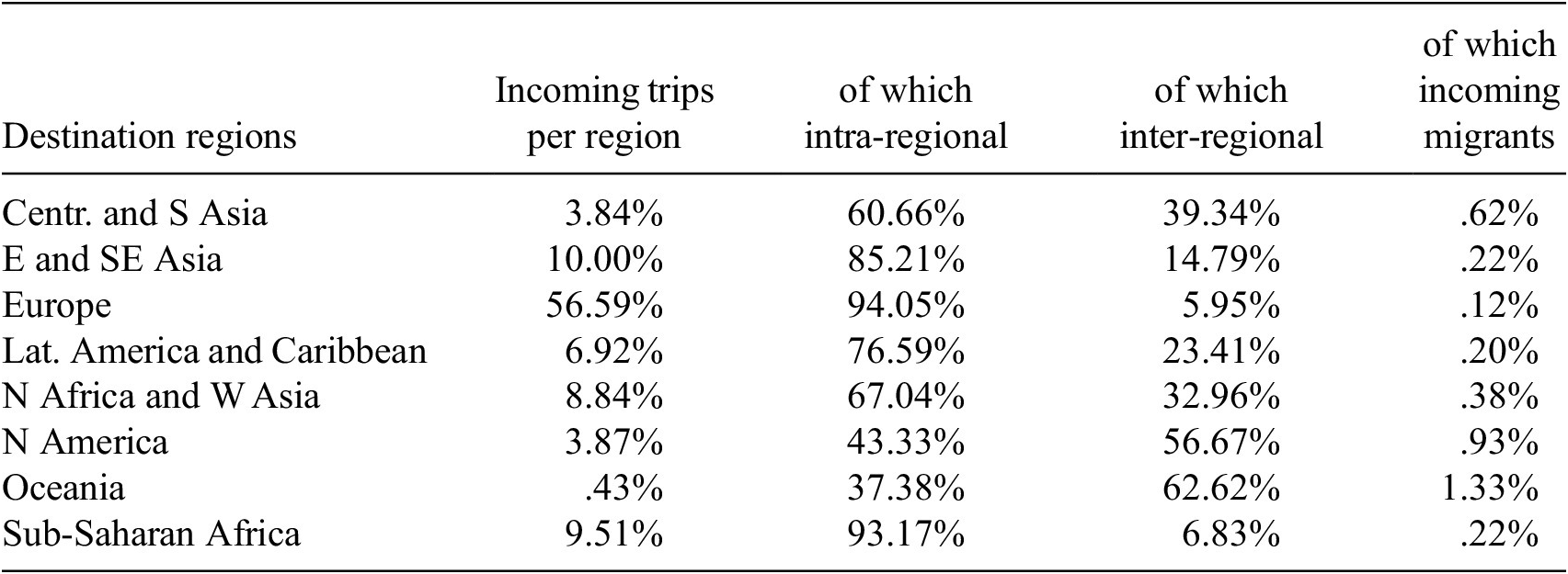


 Open access


Comments
No Comments have been published for this article.