1. Introduction
Coherent material structures are ubiquitous in a range of phenomena across multiple length scales, from oceanic and atmospheric processes (Haller Reference Haller2015; Serra et al. Reference Serra, Sathe, Beron-Vera and Haller2017, Reference Serra, Sathe, Rypina, Kirincich, Ross, Lermusiaux, Allen, Peacock and Haller2020a) to biological systems (Serra et al. Reference Serra, Streichan, Chuai, Weijer and Mahadevan2020b). In general, the coordinated motion of material parcels can be visualized by the organized patterns that tracer particles form over time (Merzkirch Reference Merzkirch2012). However, simply observing instantaneous particle positions and velocities provides an incomplete and deceptive picture – for instance, a simple change from a stationary to a rotating reference frame suffices to alter the observed coherent patterns. This motivated the development of the theory of Lagrangian coherent structures (LCSs) (Shadden Reference Shadden2012; Haller Reference Haller2015), as well as their infinitesimally short-time analogues called objective Eulerian coherent structures (Serra & Haller Reference Serra and Haller2016; Nolan, Serra & Ross Reference Nolan, Serra and Ross2020), which provide a frame-invariant framework for identifying invariant flow structures shaping observed patterns.
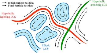
The computation of LCSs needs Lagrangian particle trajectories over a finite time interval; the resulting structures may be classified into two main groups – hyperbolic and elliptic LCSs, illustrated in figure 1. Hyperbolic LCSs can intuitively be thought of as surfaces that repel or attract neighbouring particles, leading to their binary classification as repelling or attracting LCSs, respectively. In their original definition, this repulsion or attraction must be normal to the surface and unaffected by shear. In our case, we intentionally do not make such distinction. Elliptic LCSs can intuitively be thought of as surfaces enclosing regions of coherent global dynamics, that is, regions inside of which particles move together over time. We choose to include any region of coherent material deformation, for instance jet-type structures, into our definition of elliptic LCSs. (In the original geodesic theory of LCSs, vortex-type structures are enclosed by elliptic LCSs, while jet cores in two dimensions are called parabolic LCSs (Haller Reference Haller2015).) We note that our classification of hyperbolic and elliptic LCSs is intentionally less strict than the original one (Haller Reference Haller2015) and emphasizes applicability to sparse three-dimensional experimental data from a wide range of systems beyond fluid flows (such as biological or traffic data). Together, hyperbolic and elliptic LCSs provide a comprehensive picture of coordinated motion in flow phenomena in physical and biological systems.
Sketch of the different types of LCSs that are considered in this paper. While the flow field pictured here is time-invariant to ease visualization, these structures also apply to general time-dependent flows. Note that we include any surface enclosing regions of coherent dynamics, such as vortices and jets, in our definition of elliptic LCSs.

Most of the early attempts to compute LCSs from flow data (reviewed in Hadjighasem et al. (Reference Hadjighasem, Farazmand, Blazevski, Froyland and Haller2017)) required knowledge of a dense set of particle trajectories. In practice, such a dense dataset is usually only obtainable through numerical integration of a well-resolved velocity field given by computational simulations or particle image velocimetry (PIV). Other visualization techniques such as particle tracking velocimetry provide sparser trajectories that often fall short of the required density. Furthermore, a plethora of physical and biological systems are defined not by a continuous velocity field, but rather by the dynamics of a sparse ensemble of particles in space and time; examples include drifter trajectories in the ocean (Lumpkin & Pazos Reference Lumpkin and Pazos2007), cells in living systems (Hogan Reference Hogan1999), agents in active fluids (Marchetti et al. Reference Marchetti, Joanny, Ramaswamy, Liverpool, Prost, Rao and Simha2013; Morozov Reference Morozov2017) etc. Extending computational tools for LCS identification to sparse and possibly noisy data would open the door to a wider array of potential applications, leading to a better understanding of the structure and properties of a broad class of systems.
Hyperbolic LCSs are based on the separation rate between initially close material parcels, making their identification using sparse and noisy data difficult. Their computation usually relies on the finite-time Lyapunov exponent (FTLE), which measures the sensitivity of final particle positions with respect to their initial positions (Haller Reference Haller2001; Shadden, Lekien & Marsden Reference Shadden, Lekien and Marsden2005). However, the accurate calculation of this quantity requires the trajectories of a dense and regular grid of initial particle positions, rendering its extension to sparse and noisy datasets non-trivial. Notable steps in this direction are the least-squares technique of Lekien & Ross (Reference Lekien and Ross2010) and the fitted ellipsoid approach from Rypina et al. (Reference Rypina, Getscher, Pratt and Mourre2021) for calculating the FTLE using randomly seeded particles, both of which nonetheless remain sensitive to noise as we will see later. Other methods for computing hyperbolic LCSs that accept irregular initial positions bypass the calculation of the true FTLE and can broadly be divided into two categories. In the first category, which includes the finite-time entropy (FTE) framework of Froyland & Padberg-Gehle (Reference Froyland and Padberg-Gehle2012) and the set-oriented redefinition of the FTLE by Tallapragada & Ross (Reference Tallapragada and Ross2013), the spatial domain is partitioned into a set of boxes so that local stretching measures can be computed from a discrete transfer operator that quantifies the probability of particles transferring between any two boxes over the time interval of interest (Froyland & Padberg Reference Froyland and Padberg2009). Nevertheless, their robustness to sparsity and noise in the data has not been established. The second category consists of methods computing various diagnostic quantities for locating hyperbolic LCSs from single trajectories, making them well-suited to sparse datasets. These include the complexity method (CM) of Rypina et al. (Reference Rypina, Scott, Pratt and Brown2011) measuring the ergodicity defect of trajectories, the Lagrangian descriptors (LD) of Mancho et al. (Reference Mancho, Wiggins, Curbelo and Mendoza2013) measuring trajectory length, the maximal/minimal extension of trajectories (MET) of Mundel et al. (Reference Mundel, Fredj, Gildor and Rom-Kedar2014) and the trajectory stretching exponent (TSE) of Haller, Aksamit & Encinas-Bartos (Reference Haller, Aksamit and Encinas-Bartos2021) quantifying material stretching along trajectories. Although the TSE achieves quasi-objectivity, the CM, LD and MET diagnostics are not objective and their precise relationship with material stretching is unknown. Furthermore, the robustness of all four diagnostics to sparsity and noise in the data is unclear. Finally, the encounter volume introduced in Rypina & Pratt (Reference Rypina and Pratt2017), an objective measure of mixing, has been shown to locate hyperbolic LCSs in sparse gridded datasets and can in theory be applied to randomly distributed trajectories. However, it is more closely related to diffusivity than material stretching (Rypina, Llewellyn Smith & Pratt Reference Rypina, Llewellyn Smith and Pratt2018) and its robustness to noise is also unknown.
Elliptic LCSs characterize the overall behaviour of a connected set of material parcels remaining close together over time. Taking advantage of the fact that they can be identified indirectly through the coherent sets that they enclose (Froyland, Santitissadeekorn & Monahan Reference Froyland, Santitissadeekorn and Monahan2010; Hadjighasem et al. Reference Hadjighasem, Karrasch, Teramoto and Haller2016), several techniques for identifying elliptic LCSs from sparse data have recently been proposed, most of which are reviewed in Hadjighasem et al. (Reference Hadjighasem, Farazmand, Blazevski, Froyland and Haller2017). Methods applicable to three-dimensional flows fall broadly into two categories. The first category comprises methods based on the notion of coherent set introduced in Froyland et al. (Reference Froyland, Santitissadeekorn and Monahan2010) and Froyland (Reference Froyland2013), which are regions that minimize mixing with surrounding material elements in the presence of diffusion. These sets are calculated from the transfer operator of Froyland & Padberg (Reference Froyland and Padberg2009) using a variety of techniques (Froyland & Junge Reference Froyland and Junge2015; Ser-Giacomi et al. Reference Ser-Giacomi, Rossi, López and Hernández-García2015; Williams, Rypina & Rowley Reference Williams, Rypina and Rowley2015; Banisch & Koltai Reference Banisch and Koltai2017; Froyland, Rock & Sakellariou Reference Froyland, Rock and Sakellariou2019). In the second category, individual trajectories are interpreted as points in an abstract space endowed with a certain notion of distance, and various clustering tools from computer science and statistics (Fortunato Reference Fortunato2010; Everitt et al. Reference Everitt, Landau, Leese and Stahl2011) are used to group trajectories that are close together into clusters. Such techniques differ from one another not only in the clustering algorithm they employ, but also by their definition of distance between particle trajectories. They include the application of fuzzy clustering (Froyland & Padberg-Gehle Reference Froyland and Padberg-Gehle2015), spectral graph partitioning (Hadjighasem et al. Reference Hadjighasem, Karrasch, Teramoto and Haller2016; Banisch & Koltai Reference Banisch and Koltai2017; Padberg-Gehle & Schneide Reference Padberg-Gehle and Schneide2017; Vieira, Rypina & Allshouse Reference Vieira, Rypina and Allshouse2020; Wichmann et al. Reference Wichmann, Kehl, Dijkstra and van Sebille2020; Filippi et al. Reference Filippi, Rypina, Hadjighasem and Peacock2021), spectral graph drawing (Schlueter-Kuck & Dabiri Reference Schlueter-Kuck and Dabiri2017a) and density-based clustering (Schneide et al. Reference Schneide, Pandey, Padberg-Gehle and Schumacher2018; Wichmann et al. Reference Wichmann, Kehl, Dijkstra and van Sebille2021). Outside of these two categories, Haller et al. (Reference Haller, Aksamit and Encinas-Bartos2021) also defined a quasi-objective elliptic LCS diagnostic called the trajectory rotation angle (TRA). Most of the aforementioned methods, however, struggle to consistently determine the correct number of clusters, even in simple analytical flows such as the Bickley jet (Hadjighasem et al. Reference Hadjighasem, Farazmand, Blazevski, Froyland and Haller2017). The number of clusters either is required as a heuristic input to the algorithm (that often fails as the data get sparse and/or noisy), or is dependent on the specific choice of parameters for the method. In this regard, an important improvement to the spectral clustering approach of Hadjighasem et al. (Reference Hadjighasem, Karrasch, Teramoto and Haller2016) is the automated selection procedure proposed by Filippi et al. (Reference Filippi, Rypina, Hadjighasem and Peacock2021). Finally, we note that robustness to noise and data sparsity is unclear in most of these techniques; for example, spectral clustering methods have been observed to fail at low resolutions (Schlueter-Kuck & Dabiri Reference Schlueter-Kuck and Dabiri2017a).
Here, we introduce two techniques that solve the aforementioned issues for computing hyperbolic and elliptic LCSs using sparse and noisy trajectory datasets. Our approach to compute hyperbolic LCSs follows the widely used FTLE-based definition and relies on a local least-squares fit of the flow map gradient, a tensorial quantity from which the FTLE is calculated. The least-squares procedure is similar to the technique proposed by Lekien & Ross (Reference Lekien and Ross2010), but includes two major improvements specifically targeted at coping with noise and sparsity. By feeding pairwise stretching information from all particles in a small neighbourhood around the location of interest and adding Tikhonov regularization, the method is able to alleviate the effects of both sparsity and noise while retaining enough spatial resolution to resolve the ridges in the resulting FTLE field, which locate hyperbolic LCSs. Next, our procedure to identify elliptic LCSs utilizes the same clustering algorithm as in Schneide et al. (Reference Schneide, Pandey, Padberg-Gehle and Schumacher2018) – density-based spatial clustering of applications with noise (DBSCAN) – due to its many advantages. First, it is able to tell apart trajectories belonging to coherent structures from those that do not, a feature that partition-based methods struggle to achieve (Froyland et al. Reference Froyland, Rock and Sakellariou2019; Wichmann et al. Reference Wichmann, Kehl, Dijkstra and van Sebille2021). Second, it identifies both compact structures such as vortices and elongated structures such as jets, because it assigns trajectories to clusters based on their local proximity to neighbouring trajectories in the cluster, rather than all other trajectories in the cluster as in spectral clustering (Hadjighasem et al. Reference Hadjighasem, Karrasch, Teramoto and Haller2016). Third, its implementation is straightforward due to the existence of many standard scientific libraries in which it is implemented, and it does not require a subsequent clustering step like many of the aforementioned approaches (Hadjighasem et al. Reference Hadjighasem, Karrasch, Teramoto and Haller2016; Schlueter-Kuck & Dabiri Reference Schlueter-Kuck and Dabiri2017b). Relative to the work of Schneide et al. (Reference Schneide, Pandey, Padberg-Gehle and Schumacher2018), our approach consists of the introduction of a consistent procedure for selecting the clustering parameters in DBSCAN, which constitutes a crucial step towards improving the usability of the method by practitioners. Overall, we demonstrate the robustness of our methods to different systems using both analytical and experimental data, polluted by various levels of noise and sparsity. We also provide user-friendly, lightweight Python codes that implement these techniques, allowing them to be deployed on any dataset of particle trajectories.
The paper is organized as follows. In § 2 we describe our methods for identifying hyperbolic and elliptic LCSs from sparse and noisy trajectory datasets. In § 3 these methods are applied to benchmark analytical flows as well as experimental datasets, and we conclude with some general remarks in § 4.
2. Methods
We consider a discrete set of  $N$ particles enclosed by a time-dependent body
 $\varOmega (t)$ and following the trajectories
 $\{\boldsymbol {x}^i(t)\}_{i=1}^N \in \varOmega (t) \subset \mathbb {R}^d$, where time
 $t \in [t_0,t_f]$ and
 $d$ is the spatial dimension of the system. In the following, we find it convenient to introduce the flow map
 $\boldsymbol {F}_{t_0}^t(\boldsymbol {x}_0^i) = \boldsymbol {x}^i(t)$, which takes the initial position
 $\boldsymbol {x}_0^i$ of particle
 $i$ at time
 $t_0$ to its current position
 $\boldsymbol {x}^i(t)$ at time
 $t$.
2.1. Hyperbolic coherent structures
Hyperbolic structures can be divided into two categories – intuitively, repelling and attracting LCSs are surfaces that repel or attract neighbouring particles. While a number of different theories have been proposed to identify hyperbolic LCSs in fluid flows (for reviews, see Allshouse & Peacock (Reference Allshouse and Peacock2015) and Haller (Reference Haller2015)), we propose an adaptation to sparse datasets of the original technique based on the FTLE (Haller Reference Haller2001; Shadden et al. Reference Shadden, Lekien and Marsden2005), widely used due to its simplicity.
2.1.1. Dense trajectory or velocity datasets
We first review the definition of the FTLE field in the case where the flow map  $\boldsymbol {F}_{t_0}^t(\boldsymbol {x}_0) = \boldsymbol {x}(t)$ is known for every initial position
 $\boldsymbol {x}_0 \in \varOmega (t_0)$. In practice, this condition is met when one has access to either a continuous or a finely discretized version of the entire velocity field of the system in space and time, which can be used to numerically integrate the trajectory
 $\boldsymbol {x}(t)$ of any particle.
Two particles initially located at  $\boldsymbol {x}_0$ and
 $\boldsymbol {x}_0+d\boldsymbol {x}_0$ will be separated at time
 $t$ by
 \begin{equation} \boldsymbol{F}_{t_0}^t(\boldsymbol{x}_0+d\boldsymbol {x}_0)-\boldsymbol{F}_{t_0}^t(\boldsymbol{x}_0) = \boldsymbol{\nabla} \boldsymbol{F}_{t_0}^t(\boldsymbol{x}_0) \,d\boldsymbol {x}_0+ O(|d\boldsymbol {x}_0|^2), \end{equation}
where  $\boldsymbol {\nabla } \boldsymbol {F}_{t_0}^t(\boldsymbol {x}_0)$ is the gradient of the flow map, usually computed using finite-difference techniques (Haller Reference Haller2001; Shadden Reference Shadden2012). In the limit
 $|d\boldsymbol {x}_0| \ll 1$, the ratio
 $\lambda$ of initial and final distances between these two particles is
 \begin{equation} \lambda(\boldsymbol{x}_0;d\boldsymbol {x}_0) = \frac{|\boldsymbol{F}_{t_0}^t(\boldsymbol{x}_0+d\boldsymbol {x}_0)- \boldsymbol{F}_{t_0}^t(\boldsymbol{x}_0)|}{|d\boldsymbol {x}_0|} \simeq \frac{|\boldsymbol{\nabla} \boldsymbol{F}_{t_0}^t(\boldsymbol{x}_0) \,d\boldsymbol {x}_0|}{|d\boldsymbol {x}_0|}. \end{equation}
The largest possible stretch ratio  $\lambda$ over all infinitesimal segments
 $d\boldsymbol {x}_0$ is equal to the largest singular value of the flow map gradient, which typically grows exponentially (Wiggins Reference Wiggins2003). The forward-time FTLE is defined as,
 \begin{equation} \varLambda_{t_0}^t(\boldsymbol{x}_0) = \frac{1}{t-t_0} \ln \left[ \max_{d\boldsymbol {x}_0} \lambda(\boldsymbol{x}_0;d\boldsymbol {x}_0)\right ] = \frac{1}{t-t_0} \ln \left [s_1(\boldsymbol{x}_0)\right ], \end{equation}
where  $s_1(\boldsymbol {x}_0)$ denotes the largest singular value of
 $\boldsymbol {\nabla } \boldsymbol {F}_{t_0}^t(\boldsymbol {x}_0)$. Since
 $\varLambda _{t_0}^t(\boldsymbol {x}_0)$ quantifies the rate of local material deformation, one can define the initial position of a repelling LCS over the time interval
 $[t_0,t]$ as the ridges of the scalar field
 $\varLambda _{t_0}^t(\boldsymbol {x}_0)$ (which correspond to curves in the plane and surfaces in space). Conversely, attracting LCSs can be thought of as repelling LCSs in backward time; therefore, the final position of an attracting LCS over
 $[t_0,t]$ can be defined as the ridges of the backward-time FTLE scalar field
 $\varLambda _{t}^{t_0}(\boldsymbol {x})$, where
 $\boldsymbol {x} = \boldsymbol {F}_{t_0}^t(\boldsymbol {x}_0)$.
2.1.2. Sparse and noisy trajectory datasets
The flow map gradient  $\boldsymbol {\nabla } \boldsymbol {F}_{t_0}^t$, which enters the usual definition (2.3) of the FTLE field, is inaccessible when one only has access to the trajectories of
 $N$ particles
 $\{\boldsymbol {x}^i(t)\}_{i=1}^N$. In this case, we introduce an approximation of the flow map gradient,
 $\tilde {\boldsymbol {\nabla }} \boldsymbol {F}_{t_0}^t$, which we calculate at every particle initial position
 $\boldsymbol {x}_0^i = \boldsymbol {x}^i(t_0)$ as follows. First, we draw a ball of radius
 $\delta$ around the initial position
 $\boldsymbol {x}_0^i$ of a given particle
 $i$, and call
 $\mathcal {N}$ the set of all particles
 $j$, including
 $i$ itself, such that
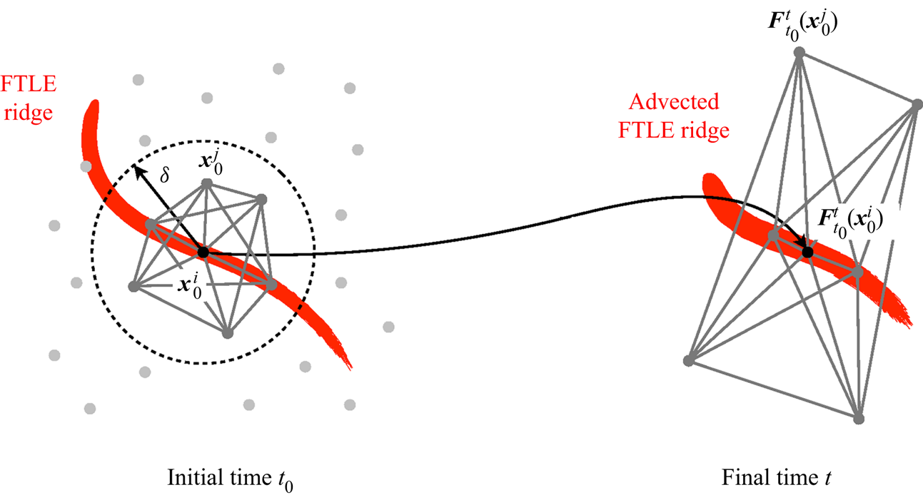
 $|\boldsymbol {x}_0^j - \boldsymbol {x}_0^i| < \delta$, as pictured in figure 2. The approximate flow map gradient at
 $\boldsymbol {x}_0^i$ is then defined such that the relation
 \begin{equation} \boldsymbol{F}_{t_0}^t(\boldsymbol{x}_0^k)-\boldsymbol{F}_{t_0}^t(\boldsymbol{x}_0^j) \simeq \tilde{\boldsymbol{\nabla}} \boldsymbol{F}_{t_0}^t(\boldsymbol{x}_0^i) [\boldsymbol{x}_0^k - \boldsymbol{x}_0^j] \end{equation}
holds for all pairs  $j,k \in \mathcal {N}, j \neq k$. Assuming that there are
 $M$ such pairs, the approximate flow map gradient can then be obtained by minimizing the square error between both sides of (2.4), resulting in the least-squares problem
 \begin{equation} \tilde{\boldsymbol{\nabla}} \boldsymbol{F}_{t_0}^t(\boldsymbol{x}_0^i) = \arg \min_{\boldsymbol{\mathsf{A}}} \,\frac{1}{M} \sum_{\substack{j,k \in \mathcal{N} \\ j \neq k}} \left\Vert \boldsymbol{\mathsf{A}} [\boldsymbol{x}_0^k - \boldsymbol{x}_0^j] - [\boldsymbol{F}_{t_0}^t(\boldsymbol{x}_0^k)-\boldsymbol{F}_{t_0}^t(\boldsymbol{x}_0^j)] \right\Vert_2^2 + {\beta} \Vert \boldsymbol{\mathsf{A}} - \boldsymbol{\mathsf{I}} \Vert_F^2, \end{equation}
where  $\boldsymbol{\mathsf{A}} \in \mathbb{R}^{d \times d}$,
 $\boldsymbol{\mathsf{I}} \in \mathbb{R}^{d \times d}$ is the identity matrix,
 $\Vert \cdot \Vert _2$ and
 $\Vert \cdot \Vert _F$ denote the Euclidian and Frobenius norms, respectively, and
 $\beta$ is a regularization parameter that biases
 $\tilde {\boldsymbol {\nabla }} \boldsymbol {F}_{t_0}^t$ towards the identity in the absence of data, which corresponds to classical Tikhonov regularization (Kaipio & Somersalo Reference Kaipio and Somersalo2006). As shown in Appendix A, the solution of the above minimization problem is given by
 \begin{equation} \tilde{\boldsymbol{\nabla}}
\boldsymbol{F}_{t_0}^t(\boldsymbol{\mathsf{x}}_0^i) =
(\boldsymbol{\mathsf{Y}} \boldsymbol{\mathsf{X}}^{\mathrm{T}} + \beta M
\boldsymbol{\mathsf{I}}) (\boldsymbol{\mathsf{X}} \boldsymbol{\mathsf{X}}^{\mathrm{T}}
+ \beta M \boldsymbol{\mathsf{I}})^{{-}1}, \end{equation}
where the matrices  $\boldsymbol{\mathsf{X}}, \boldsymbol{\mathsf{Y}} \in \mathbb {R}^{d \times M}$ are defined as
 $$\begin{gather} {\boldsymbol{\mathsf{X}}} = \left[ \dots \, | \, ({\boldsymbol{x}}_0^k - \boldsymbol{x}_0^j) \, | \, \dots \right], \end{gather}$$
 $$\begin{gather}\boldsymbol{\mathsf{Y}} = \left[ \dots \, | \, (\boldsymbol{F}_{t_0}^t(\boldsymbol{x}_0^k)-\boldsymbol{F}_{t_0}^t(\boldsymbol{x}_0^j)) \, | \, \dots \right], \end{gather}$$
for all pairs  $j,k \in \mathcal {N}, j \neq k$. While our approach is reminiscent of the work of Lekien & Ross (Reference Lekien and Ross2010) to compute FTLEs on unstructured meshes, important differences include the specific set of particle pairs considered in the least-squares problem (2.5), and the addition of a regularization term. We now replace
 $s_1(\boldsymbol {x}_0)$ in (2.3) with
 $\tilde {s}_1(\boldsymbol {x}_0^i)$, the largest singular value of the approximate flow map gradient
 $\tilde {\boldsymbol {\nabla }} \boldsymbol {F}_{t_0}^t(\boldsymbol {x}_0^i)$ obtained from (2.6), which yields the approximate forward-time FTLE at the particle position
 $\boldsymbol {x}_0^i$:
 \begin{equation} \tilde{\varLambda}_{t_0}^t(\boldsymbol{x}_0^i) = \frac{1}{t-t_0} \ln \left [\tilde{s}_1(\boldsymbol{x}_0^i)\right]. \end{equation}
Finally, the approximate initial positions of repelling LCSs over  $[t_0,t_f]$ can be defined as the ridges of the forward-time discrete FTLE
 $\tilde {\varLambda }_{t_0}^t(\boldsymbol {x}_0^i)$. Conversely, the approximate final positions of attracting LCSs over
 $[t_0,t_f]$ can be defined as the ridges of the backward-time discrete FTLE
 $\tilde {\varLambda }_t^{t_0}(\boldsymbol {x}_t^i)$, where
 $\boldsymbol {x}_t^i = \boldsymbol {x}^i(t)$ are the final particle positions, and the set
 $\mathcal {N}$ now comprises all particles
 $j$, including
 $i$ itself, such that
 $|\boldsymbol {x}_t^j - \boldsymbol {x}_t^i| < \delta$.
Identification of hyperbolic repelling LCSs. The flow map gradient is approximated as the least-squares fit of the tensor that maps the initial positions of segments relating  $\boldsymbol {x}_0^i$ and its neighbours in a neighbourhood of radius
 $\delta$ to their final positions.

Fitting a linear operator to map the local evolution of material vectors was introduced by, among others, Falk & Langer (Reference Falk and Langer1998) to study shear deformation in amorphous solids, and applied by Schall, Weitz & Spaepen (Reference Schall, Weitz and Spaepen2007) to study structural rearrangements in colloidal glasses and by Kelley & Ouellette (Reference Kelley and Ouellette2011) to study mixing in fluid flows. However, our technique is most closely related to the work of Lekien & Ross (Reference Lekien and Ross2010), who performed an analytical least-squares fit of the flow map gradient similar to (2.6) in order to compute the FTLE field on unstructured meshes. Relative to Lekien & Ross (Reference Lekien and Ross2010), we introduce two modifications that are specifically targeted at improving results in the presence of noise and sparsity. The first is to take into account all particle pairs in a ball of finite radius around  $\boldsymbol {x}_0^i$ instead of only the pairs linking
 $\boldsymbol {x}_0^i$ to its immediate neighbours, which greatly increases the amount of data available. The second is to add Tikhonov regularization to the minimization problem (2.5), which helps numerically stabilize the solution when the problem is poorly conditioned. Taken together, these two improvements are effective at smoothing out noise while retaining signal, as we will see later in various examples.
Parameter selection strategy. Our approximation scheme contains two free parameters  $\beta$ and
 $\delta$. Although both play a role in reducing the effect of noise, they do so in different ways – a large
 $\beta$ gives less weight to the data-dependent term in (2.5), while a large radius
 $\delta$ results in a larger set
 $\mathcal {N}$ of particles. In practice, we have found that
 $\delta$ is much more effective than
 $\beta$ at countering the effect of noise in the data. Thus, we choose a value
 $\beta \ll r^2$ that only serves to regularize the least-squares solution (2.6) in the degenerate case where
 $\boldsymbol{\mathsf{X}} \boldsymbol{\mathsf{X}}^{\mathrm {T}}$ is ill-conditioned. Here,
 $r$ is the average initial distance between neighbouring particles, which can be estimated as
 $r \simeq \sqrt {A_0/N}$ for two-dimensional datasets and
 $r \simeq \sqrt [3]{V_0/N}$ for three-dimensional datasets, where
 $A_0$ and
 $V_0$ are respectively the initial area and initial volume of the system and
 $N$ is the number of particles. In the examples to follow, we simply select
 $\beta = 10^{-10} r$. As for the radius
 $\delta$, it should be sufficiently large that enough particle pairs are included in the least-squares fit (2.6), but not so large that particle pairs belonging to qualitatively different regions of the flow are lumped together. The former is quantified by a length scale of the order of
 $r$, while the latter is quantified by the characteristic length scale
 $\ell$ of flow features. We therefore choose
 $\delta$ by starting from a value equal to
 $r$ and slowly increasing it until ridges emerge from the computed FTLE field, knowing that
 $\delta$ should not exceed
 $\ell$ (or the domain size when
 $\ell$ is unknown). If no clean ridges appear, then the dataset is either too sparse and/or noisy for hyperbolic LCSs to be detected, or does not contain any. This procedure is illustrated with various examples in § 3.
2.2. Elliptic coherent structures
Intuitively, elliptic LCSs are surfaces enclosing regions of coherent motion in which particles remain close together. Here, we consider such coherent regions to comprise both vortex-type structures and elongated jet-type structures. As is the case for hyperbolic LCSs, there exist many different techniques for identifying elliptic LCSs in fluid flows, usually through the coherent regions that they enclose (for a review, see Hadjighasem et al. (Reference Hadjighasem, Farazmand, Blazevski, Froyland and Haller2017)).
As mentioned in the introduction, we focus on the class of methods that interpret individual trajectories as points in an abstract space endowed with a certain notion of distance, before using a clustering tool to identify coherent regions as clusters of trajectories that remain close over the considered time interval. Following Hadjighasem et al. (Reference Hadjighasem, Karrasch, Teramoto and Haller2016), we define the distance  $d_{ij}$ between two trajectories
 $\boldsymbol {x}_i(t)$ and
 $\boldsymbol {x}_j(t)$ as the time average
 \begin{equation} d_{ij} = \frac{1}{t-t_0} \int_{t_0}^t \Vert \boldsymbol{x}^i(t') - \boldsymbol{x}^j(t') \Vert \,{\rm d}t'. \end{equation}
Treating trajectories like individual points, we then apply the DBSCAN algorithm introduced by Ester et al. (Reference Ester, Kriegel, Sander and Xu1996), which was first utilized to detect coherent sets of trajectories in Schneide et al. (Reference Schneide, Pandey, Padberg-Gehle and Schumacher2018). We complement prior work via the introduction of a parameter selection strategy, thereby improving the usability of the method since choosing parameters is a critical aspect of any clustering algorithm.
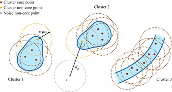
The DBSCAN algorithm is implemented in many scientific libraries, making it quick and easy to run, and can be abstracted as shown in Algorithm 1 (Schubert et al. Reference Schubert, Sander, Ester, Kriegel and Xu2017). Given a set of points in some metric space, the algorithm assigns points to clusters based on their local proximity to a given number of other points in the cluster rather than all of them. This produces groups defined by a minimum density throughout rather than proximity between all member points. The minimum density is set by the parameters  $\texttt {minPts}$ and
 $\texttt {eps}$: a minimum number
 $\texttt {minPts}$ of points must belong to the same ball of radius
 $\texttt {eps}$ in order to be part of the same cluster, as illustrated in figure 3 for
 $\texttt {minPts} = 3$ and the radius
 $\texttt {eps}$ indicated by the circles. As a result, DBSCAN is not only able to identify both compact and elongated structures, but it also has an inherent ability to designate points that do not belong to any cluster, lying alone in low-density regions, as ‘noise’. (Here, ‘noise’ does not mean that these points are physically irrelevant; rather, it refers to the fact that they do not belong to any cluster.) Such property is desirable since not every point is necessarily part of a cluster. When applying DBSCAN to our dataset of particle trajectories using the distance metric (2.10), the resulting clusters identify groups of particles with coherent motion (such as vortices and jets) and enclosed by elliptic LCSs, with ‘noise’ particles in between separating them; see figure 3. In practice, we use the scikit-learn implementation of the DBSCAN algorithm in Python (Pedregosa et al. Reference Pedregosa2011). We provide below a consistent methodology for the choice of the parameters
 $\texttt {minPts}$ and
 $\texttt {eps}$.
Identification of elliptic LCSs. The DBSCAN algorithm is applied to a set of points representing individual particle trajectories and separated by the distance defined in (2.10). It then identifies elliptic LCSs as clusters of trajectories that are close to each other.

DBSCAN (abstract form)

Parameter selection strategy. The parameter  $\texttt {minPts}$ is the easiest to set and we follow the recommendation of the authors of the DBSCAN algorithm to set it to twice the dimensionality d of the dataset (Sander et al. Reference Sander, Ester, Kriegel and Xu1998; Schubert et al. Reference Schubert, Sander, Ester, Kriegel and Xu2017) – that is,
 $\texttt {minPts} = 4$ and
 $6$ for two- and three-dimensional data, respectively. The parameter
 $\texttt {eps}$ is harder to choose, with a consensus on a specific heuristic still missing (Schubert et al. Reference Schubert, Sander, Ester, Kriegel and Xu2017). Here, we propose a way to pick
 $\texttt {eps}$ by appealing to a well-known concept in data clustering, which stipulates that an appropriate choice of parameters is one for which the corresponding results are most stable, i.e. robust with respect to perturbations in the data or parameters (von Luxburg Reference von Luxburg2010). Our strategy then comprises two steps: first, we eliminate (i.e. classify as noise) spurious clusters, which are those clusters whose size is highly sensitive to
 $\texttt {eps}$ and tend to disappear for larger
 $\texttt {minPts}$; second, we pick a value of
 $\texttt {eps}$ around which the size of the remaining, physically meaningful clusters is stable. As a guide to the search process,
 $\texttt {eps}$ should be of the order of the average distance
 $d_{ij}$ between every particle trajectory and its
 $(\texttt {minPts}-1)$th nearest neighbour. We describe in detail the practical application of this methodology to various datasets in § 3.
3. Results
We now apply our algorithms for the detection of hyperbolic and elliptic LCSs to four different systems. The first two, the Bickley jet and Arnold–Beltrami–Childress (ABC) flow, are described by analytic velocity fields and are frequently used as benchmark problems for the detection of coherent structures (Hadjighasem et al. Reference Hadjighasem, Karrasch, Teramoto and Haller2016, Reference Hadjighasem, Farazmand, Blazevski, Froyland and Haller2017). We use the known velocity fields to calculate trajectory data from randomly seeded particles with artificially introduced noise, and we compare the LCSs identified by our methods with the ground truth. The third and fourth systems, motile cells in a developing chicken embryo, and ocean tracers in the Gulf of Mexico, correspond to experimental data from developmental biology and oceanography respectively, and highlight the capability of our methods to identify structures from sparse and noisy trajectory data in widely differing applications.
In the case of the Bickley jet and ABC flow, we present results using higher-resolution data when identifying hyperbolic LCSs than when extracting elliptic LCSs. While our methods for detecting hyperbolic and elliptic LCSs can be applied to data of the same resolution, we study them at different resolution levels because results for elliptic LCSs are consistently better than results for hyperbolic LCSs at a given resolution, for both two- and three-dimensional flows. This is a consequence of the fact that our method for detecting hyperbolic LCSs is based on the approximation (2.4) of the flow map gradient  $\boldsymbol {\nabla } \boldsymbol {F}$, which only involves trajectories that are initially close to one another. On the other hand, our method for detecting elliptic LCSs finds clusters based on the time-averaged distance (2.10) between all pairs of trajectories. Thus, the computation of hyperbolic LCSs naturally requires data at a higher resolution than for elliptic LCSs.
3.1. Bickley jet
The Bickley jet is an analytical model of a two-dimensional meandering zonal jet separating counterrotating vortices in the Earth's atmosphere (del Castillo-Negrete & Morrison Reference del Castillo-Negrete and Morrison1993; Rypina et al. Reference Rypina, Brown, Beron-Vera, Koçak, Olascoaga and Udovydchenkov2007). The time-dependent flow field is described by the streamfunction  $\psi (x,y,t) = \psi _0(y) + \psi _1(x,y,t)$, where
 $$\begin{gather} \psi_0(y) = c_3 y - UL \tanh (y/L), \end{gather}$$
 $$\begin{gather}\psi_1(x,y,t) = UL \, \mathrm{sech}^2 (y/L) \sum_{n=1}^3 \epsilon_n \cos(k_n(x - \omega_n t)). \end{gather}$$
In order to facilitate comparison, we use the same parameter values as in Schlueter-Kuck & Dabiri (Reference Schlueter-Kuck and Dabiri2017a); that is,  $U = 62.66~\mathrm {m}~\mathrm {s}^{-1}$,
 $L = 1.77 \times 10^6~ \mathrm {m}$,
 $k_n = 2n/r_0$ where
 $r_0 = 6.371 \times 10^6~ \mathrm {m}$ is the radius of the Earth,
 $\epsilon = [0.0075, 0.15, 0.3]$,
 $c = [0.1446, 0.205, 0.461] U$ and
 ${\omega } = c - c_3$. The flow is computed in the
 $x$-periodic domain
 $\varOmega = [0,{\rm \pi} r_0] \times [-3,3] 10^6~\mathrm {m}$. In the following, all distances are measured in units of in
 $10^6~\mathrm {m}$ and time is measured in days. The streamlines produced at
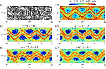
 $t=0$ by these parameter values are depicted in figure 4(a), and show the existence of three pairs of counterrotating vortices separated by a meandering horizontal jet. The streamfunction and parameter values considered here produce the same flow field as that studied in Hadjighasem et al. (Reference Hadjighasem, Farazmand, Blazevski, Froyland and Haller2017), but viewed in a reference frame translating at the constant speed of the vortices.
Hyperbolic repelling LCSs in the Bickley jet. (a) Streamlines at  $t=0$, (b) exact continuous FTLE field over the time window
 $t \in [0,40]$, (c–f) discrete FTLE field computed over the same time window using 6000 particles with (c)
 $\sigma = 0$,
 $\delta = 0.3$, (d)
 $\sigma = 0$,
 $\delta = 0.5$, (e)
 $\sigma = 0.2$,
 $\delta = 0.3$ and (f)
 $\sigma = 0.2$,
 $\delta = 0.5$. Here,
 $\sigma$ refers to the standard deviation of observation noise and
 $\delta$ is the neighbourhood radius used in the least-squares fit of the flow map gradient. The colourbar is shared for plots (b–f), and values above 0.16 are shown in the same colour.

We first compute repelling LCSs in the Bickley jet over the time window  $t \in [0,40]$, visualized by the ridges of the forward FTLE field at initial time. As a benchmark, figure 4(b) displays the reference FTLE field
 $\varLambda _0^{40}$, computed through a finite-difference approximation of the flow map gradient (Shadden Reference Shadden2012) using a set of noise-free particle trajectories initialized on a
 $300 \times 90$ rectangular grid. The trajectories were integrated from the velocity field using a fourth-order Runge–Kutta method with tolerance
 $10^{-6}$, as is the case for all trajectory calculations in the remainder of the paper. We note that for the purpose of evaluating the flow map gradient, we let trajectories leave the initial domain
 $\varOmega$ despite the periodicity in the
 $x$ direction. Indeed, the flow map gradient relates the initial and final values of the separation vector between infinitesimally close trajectories. Since this separation vector lives in the so-called ‘tangent space’ of
 $\varOmega$, which is devoid of any periodicity, the flow map gradient is better approximated by evaluating the difference between unbounded trajectories.
When working with particle trajectories from experimental data that are both sparse and associated with random initial locations, we need to modify the finite-difference methodology utilized to deduce the results in figure 4(b). To simulate such a scenario using the Bickley jet, we compute trajectories for 6000 particles (that is, 22 % of the gridded data used in figure 4b) whose initial positions are randomly assigned through a spatially uniform distribution function, and we add white Gaussian noise of standard deviation  $\sigma$ to all trajectories to simulate observation noise in real data. Figure 4(c–f) shows the discrete FTLE field
 $\tilde {\varLambda }_0^{40}$ for different values of
 $\sigma$ and the neighbourhood radius
 $\delta$. In a manner similar to the continuous FTLE field in figure 4(b), these discrete FTLE fields also display the two ridges separating the meandering jet from the vortices. In the absence of noise, a smaller value of
 $\delta$ enables a finer delineation of the ridges. However, in the presence of noise, increasing
 $\delta$ leads to an effective averaging that reduces the pollution caused by the noise and yields cleaner ridges, due to the additional data used in the least-squares fit of the flow map gradient at every point. Therefore,
 $\delta$ controls a trade-off between the ridges’ width and their pollution from noise. Because its optimal value depends on the inherent spatial resolution and noisiness of the data,
 $\delta$ should in practice be slowly increased until clean ridges emerge from the computed FTLE field, but not made too large that it will eventually smear the ridges. This beneficial effect of
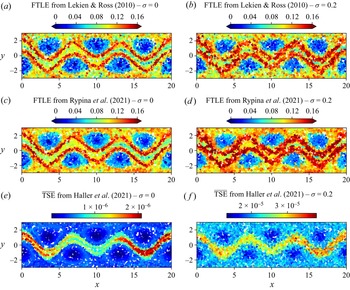
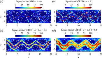
 $\delta$ in the presence of noise is evidenced in Appendix E, where we apply three alternative techniques for the identification of hyperbolic structures in sparse datasets to the same data. These techniques, however, do not have a built-in mechanism to deal with noise and therefore lead to worse results in the presence of the latter. Further, in Appendix F, we analyse the same dataset through the lens of relative dispersion, a common metric in oceanography (Provenzale Reference Provenzale1999), and a generalization thereof. Our method once again leads to better results. Finally, we note that similarly to the vast majority of existing techniques for hyperbolic LCS detection, we do not propose an automated algorithm to numerically extract the ridges from the computed FTLE field.
We turn to the computation of elliptic LCSs over  $t \in [0,40]$. The FTLE in figure 4(b) suggests the existence of such structures enclosing seven regions of the flow – each of the six vortices as well as the meandering jet, which has been confirmed by distinct methods (Hadjighasem et al. Reference Hadjighasem, Farazmand, Blazevski, Froyland and Haller2017; Vieira et al. Reference Vieira, Rypina and Allshouse2020; Wichmann et al. Reference Wichmann, Kehl, Dijkstra and van Sebille2021). We consider 1080 particles initialized on a rectangular grid and pollute their trajectories with white Gaussian noise of standard deviation
 $\sigma$. We then apply the clustering approach described in § 2.2 to uncover the elliptic LCSs. In particular, we account for the periodicity of the domain in the
 $x$ direction when calculating
 $d_{ij}$ given by (2.10). Because the periodicity of the domain sets an upper bound on
 $d_{ij}$, this makes it more difficult for the clustering algorithm to discriminate between particles belonging to different groups of coherent motion. (For instance, the value of
 $d_\textit {ij}$ between a particle trajectory in the meandering jet and another in one of the vortices will be much smaller than if we did not account for domain periodicity due to the much faster horizontal velocity of the jet. This smaller value would then be closer to the value of
 $d_{ij}$ between two particle trajectories in the same vortex.) Some of the previous attempts at calculating elliptic LCSs using clustering algorithms did not account for such periodicity in the calculation of pairwise distances (Hadjighasem et al. Reference Hadjighasem, Karrasch, Teramoto and Haller2016; Schlueter-Kuck & Dabiri Reference Schlueter-Kuck and Dabiri2017a). Finally, we note that the clustering results are largely insensitive to small perturbations in the initial positions of the particles; thus a rectangular grid was chosen simply in order to aid the visualization of the computed structures.
Following our parameter selection strategy, we now select appropriate values for the clustering parameters  $\texttt {eps}$ and
 $\texttt {minPts}$. We choose
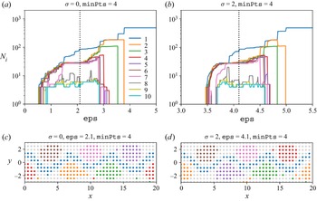
 $\texttt {minPts} = 4$ since the dataset is two-dimensional, and apply repeatedly the DBSCAN algorithm sweeping through a range of values of
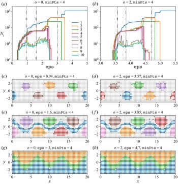
 $\texttt {eps}$. Beginning with the noise-free data, figure 5(a) shows the number
 $N_i$ of particles in each of the ten largest groups identified by DBSCAN as a function of
 $\texttt {eps}$. The algorithm classifies all particles as noise (i.e. not part of any coherent group) for
 $\texttt {eps} = 0$, and lumps all particles into one unique group for large
 $\texttt {eps}$. This behaviour is expected given that DBSCAN creates groups characterized by the presence of at least
 $\texttt {minPts}$ neighbouring particles in a neighbourhood of radius
 $\texttt {eps}$. As
 $\texttt {eps}$ is varied in between these two extremes, we observe two categories of groups. Groups 1 to 7 contain a rather stable number of particles over a wide range of
 $\texttt {eps}$, while the size of groups 8 to 10 is highly sensitive to
 $\texttt {eps}$. Furthermore, Appendix B shows that repeating the same calculation for higher values of
 $\texttt {minPts}$ leads to the disappearance of groups 8 to 10. Thus, the first category contains physically meaningful groups, while the second category contains spurious groups that we henceforth discard (that is, assign to noise) in the following plots. (For ease of visualization, we only displayed the size of the ten largest groups. In this example, this choice is inconsequential since there cannot be a physically meaningful group of a higher index (i.e. smaller size) than a spurious group. It therefore suffices to determine that a group of a given index is spurious to know that all other groups with a higher index are spurious as well. Of course, if a dataset were such that the ten largest groups are all meaningful then it would be necessary to monitor groups with higher indexes until a spurious group is found.) Figure 5(c,e,g) displays the coherent groups identified by DBSCAN for the three different values of
 $\texttt {eps}$ shown as the dotted lines in figure 5(a); particles classified as noise are shown in grey. A small
 $\texttt {eps}$ merely identifies the vortex cores while a large
 $\texttt {eps}$ detects the meandering jet but not the vortices. Thus,
 $\texttt {eps}$ sets the coherence length scale of the identified structures, as Wichmann et al. (Reference Wichmann, Kehl, Dijkstra and van Sebille2021) noticed with the OPTICS algorithm, itself a generalization of DBSCAN. According to our parameter selection strategy, we should pick a value of
 $\texttt {eps}$ around which the size of the physically meaningful groups 1 to 7 is stable, which is true for any value of
 $\texttt {eps}$ in the range 1.4 to 1.8. In particular, the clustering result obtained for
 $\texttt {eps} = 1.6$ identifies all known elliptic LCSs in the Bickley jet and therefore validates our methodology for the choice of
 $\texttt {eps}$. (The few seemingly outlier particles away from the green and orange clusters in figure 5(
 $e$) correctly belong to the assigned groups, as demonstrated in Appendix C.) Supplementary movie 1 available at https://doi.org/10.1017/jfm.2022.652 shows the Lagrangian evolution of the particles in figure 5(e), and the identified groups are observed to remain coherent throughout the time window. Note that Hadjighasem et al. (Reference Hadjighasem, Farazmand, Blazevski, Froyland and Haller2017) applied several techniques for detecting elliptic LCSs to the Bickley jet, and none of them was able to identify simultaneously all six coherent vortices and the meandering jet.
Elliptic LCSs in the Bickley jet. (a,b) Number  $N_i$ of particles in each of the ten largest groups identified by the DBSCAN algorithm as a function of the parameter
 $\texttt {eps}$ for
 $\texttt {minPts} = 4$. The data consist of 1080 particle trajectories advected over
 $t \in [0,40]$ and artificially polluted by observation noise of standard deviation (a)
 $\sigma = 0$ and (b)
 $\sigma = 2$. (c–h) Coherent groups identified by DBSCAN for (c,e,g)
 $\sigma = 0$ and (d,f,h)
 $\sigma = 2$ using different values of
 $\texttt {eps}$ shown as the dotted lines in (a,b). Supplementary movie 1 shows the Lagrangian evolution of the particles in (e).

We then consider the effect of observation noise. Figure 5(b,d,f,h) is the counterpart of figure 5(a,c,e,g), with white Gaussian noise of standard deviation  $\sigma = 2$ applied to each computed particle trajectory. To facilitate visualization, the particles in figure 5(d,f,h) are displayed at their true initial location without the applied noise. Despite the intensity of the noise, the coherent groups identified by the clustering algorithm are very similar to their noise-free counterparts. The main difference is that similar clustering results correspond to higher values of
 $\texttt {eps}$ in the presence of noise, but our methodology itself is robust to noise.
Finally, in Appendix D we present an analysis similar to that carried out in this section, using fewer particle trajectories. The results demonstrate the robustness of our algorithms and parameter selection strategy to various amounts of noise and sparsity in the data.
3.2. ABC flow
For our second analytical example, we consider the ABC flow, a family of exact three-dimensional solutions of Euler's equation given by the steady velocity field
 $$\begin{gather} \dot{x} = A \sin z + C \cos y, \end{gather}$$
 $$\begin{gather}\dot{y} = B \sin x + A \cos z, \end{gather}$$
 $$\begin{gather}\dot{z} = C \sin y + B \cos x. \end{gather}$$
We employ the same parameter values  $A = \sqrt {3}$,
 $B = \sqrt {2}$ and
 $C = 1$ considered in previous studies (Dombre et al. Reference Dombre, Frisch, Greene, Hénon, Mehr and Soward1986; Haller Reference Haller2001) and set the domain to be the three-dimensional torus
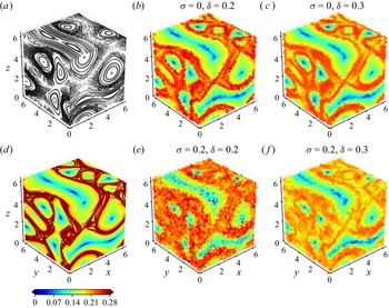
 $\varOmega = [0,2{\rm \pi} ]^3$ with periodic boundary conditions (Dombre et al. Reference Dombre, Frisch, Greene, Hénon, Mehr and Soward1986; Froyland & Padberg Reference Froyland and Padberg2009). Figure 6(a) shows three orthogonal Poincaré sections of 100 trajectories initialized on each face of the cube and advected over
 $t \in [0,2000]$. These Poincaré sections confirm the existence of six regions of coherent motion separated by a chaotic background, as previously reported in the literature (Dombre et al. Reference Dombre, Frisch, Greene, Hénon, Mehr and Soward1986; Budišić & Mezić Reference Budišić and Mezić2012; Hadjighasem et al. Reference Hadjighasem, Karrasch, Teramoto and Haller2016).
Hyperbolic repelling LCSs in the ABC flow. (a) Poincaré maps for integration time  $t \in [0,2000]$, (d) exact continuous FTLE field over the time window
 $t \in [0,20]$, (b,c,e, f) discrete FTLE field computed over the same time window using 120 000 particles with (b)
 $\sigma = 0$,
 $\delta = 0.2$, (c)
 $\sigma = 0$,
 $\delta = 0.3$, (e)
 $\sigma = 0.2$,
 $\delta = 0.2$ and (f)
 $\sigma = 0.2$,
 $\delta = 0.3$. Here,
 $\sigma$ refers to the standard deviation of observation noise and
 $\delta$ is the neighbourhood radius used in the least-squares fit of the flow map gradient. The colourbar is shared for plots (b–f), and values below 0 and above 0.28 are shown in the same colour.

We first compute the repelling LCSs in the ABC flow over the time window  $t \in [0,20]$, visualized by the ridges of the forward FTLE field. Figure 6(d) displays the reference FTLE field
 $\varLambda _0^{20}$ at initial time, computed by finite-differencing the flow map obtained through advection of a dense rectangular initial lattice of
 $200 \times 200 \times 200$ particles. Similar to our treatment of the Bickley jet, we let the trajectories leave the initial domain
 $\varOmega$ when evaluating the flow map gradient. As expected, the FTLE ridges fill the chaotic zone and bound the regions of coherent motion revealed by the Poincaré sections in figure 6(a). We then simulate sparse experimental data by computing the trajectories of 120 000 particles (that is, 1.5 % of the gridded data used in figure 6d) randomly initialized in
 $\varOmega$ following a spatially uniform distribution, and we add white Gaussian noise of standard deviation
 $\sigma$ to all trajectories. Figure 6(b,c,e,f) shows the discrete FTLE field
 $\tilde {\varLambda }_0^{20}$ for different values of
 $\sigma$ and the neighbourhood radius
 $\delta$. As we observed with the Bickley jet, a smaller value of
 $\delta$ enables a finer delineation of the ridges in the absence of noise. However, in the presence of noise, increasing
 $\delta$ reduces the pollution caused by the noise and leads to cleaner ridges. These results confirm the important role played by the parameter
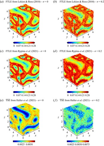
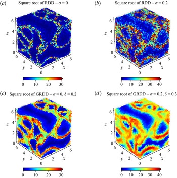
 $\delta$ in the case of three-dimensional data as well. Note that due to the long integration time considered here, the discrete FTLE ridges fill out the chaotic region, therefore outlining the boundary between the latter and the coherent vortices. In Appendix E, we apply three alternative techniques for the identification of hyperbolic structures in sparse datasets to the same data. As we already observed with the Bickley jet, these techniques do not have a built-in mechanism to deal with noise and therefore lead to worse results in the presence of the latter. We also analyse in Appendix F the same dataset through the lens of relative dispersion and a generalization thereof. As in the case of the Bickley jet, our method once again leads to better results.
We then turn to the computation of elliptic LCSs over  $t \in [0,20]$, which should reveal the six coherent vortices that are seen in figure 6(a). We compute trajectories for a set of 15 625 particles initialized on a rectangular lattice, to which we add white Gaussian noise of standard deviation
 $\sigma$. We then apply the clustering approach and parameter selection strategy described in § 2.2 to uncover the elliptic LCSs. We choose
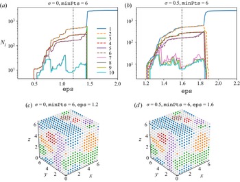
 $\texttt {minPts} = 6$ since the dataset is three-dimensional, and apply repeatedly the DBSCAN algorithm using a range of values of
 $\texttt {eps}$. Beginning with the case
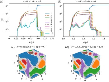
 $\sigma = 0$, figure 7(a) shows the number
 $N_i$ of particles in each of the ten largest groups identified by DBSCAN as a function of
 $\texttt {eps}$. We first discard groups 7 to 10 (and above) as their size is highly sensitive to
 $\texttt {eps}$, and they tend to disappear for larger values of
 $\texttt {minPts}$ as shown in Appendix B. The number of remaining physically meaningful groups and their size remain stable for
 $\texttt {eps}$ in the range 0.6 to 0.9. We thus pick
 $\texttt {eps} = 0.7$ and plot the corresponding clusters in figure 7(c). These identify each of the six coherent vortices that appear in figure 6(a), providing a validation of our methodology in the case of three-dimensional chaotic flows. Supplementary movie 2 shows the Lagrangian evolution of the particles in figure 7(c), highlighting how trajectories belonging to the coherent groups behave very differently from those in the incoherent group, despite starting initially very close. Corresponding results with white Gaussian noise of standard deviation
 $\sigma = 0.5$ are shown in figure 7(b,d). The particles in figure 7(
 $d$) are displayed at their true initial noise-free location, to facilitate visualization. Once again, the similarity between the clusters obtained with and without noise exemplifies the robustness of both the algorithm and the parameter selection methodology.
Elliptic LCSs in the ABC flow. (a,b) Number  $N_i$ of particles in each of the ten largest groups identified by the DBSCAN algorithm as a function of the parameter
 $\texttt {eps}$, for
 $\texttt {minPts} = 6$. The data consist of 15 625 particle trajectories advected over
 $t \in [0,20]$ and artificially polluted by observation noise of standard deviation (a)
 $\sigma = 0$ and (b)
 $\sigma = 0.5$. (c,d) Coherent groups identified by DBSCAN for (c)
 $\sigma = 0$ and (d)
 $\sigma = 0.5$, using the value of
 $\texttt {eps}$ shown as the dotted line in (a,b). Supplementary movie 2 shows the Lagrangian evolution of the particles in (c).

Because of the ability of the DBSCAN algorithm to scale up to a large number of particles, our approach does not require sparsification of the weighted graph as opposed to the spectral clustering methodology of Hadjighasem et al. (Reference Hadjighasem, Karrasch, Teramoto and Haller2016). For the number of particles we consider, the DBSCAN algorithm runs in a mere few seconds (on a personal laptop from 2015) once the edge weights (2.10) are computed. Further, contrary to Hadjighasem et al. (Reference Hadjighasem, Karrasch, Teramoto and Haller2016), we account for the periodicity of the domain when calculating the pairwise distances in (2.10), which makes it more difficult for the clustering algorithm to discriminate between particles belonging to different groups of coherent motion.
Finally, in Appendix D we carry out a similar analysis using fewer particle trajectories. The results demonstrate the robustness of our algorithms and parameter selection strategy to various amounts of noise and sparsity in the data.
3.3. Chicken embryo
For our third example, we consider the global deformation and flow of tissue in a developing chicken embryo. The experimental data, acquired by Rozbicki et al. (Reference Rozbicki, Chuai, Karjalainen, Song, Sang, Martin, Knölker, MacDonald and Weijer2015), consists of a velocity field tracking the coordinated motion of thousands of cells during a key embryonic phase known as gastrulation. This phase is characterized by the formation of the primitive streak, a structure that marks the onset of formation of multiple tissue layers and the establishment of the overall body plan during the early stages of development (Stern Reference Stern2004). The velocity field was obtained by imaging a live chicken embryo at regular intervals of time using light-sheet microscopy, and feeding the resulting high-resolution images of moving cells to a PIV algorithm. This process was carried out over a period of 12 h, spanning the whole formation of the primitive streak.
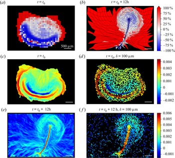
We begin by visualizing the tissue deformation during formation of the primitive streak. To this effect, we advect the square tissue domains shown at initial time in figure 8(a) using the PIV-derived velocity field, resulting in the deformed domains shown in figure 8(b) at final time. The domains are coloured according to their percentage volume change over the course of the 12 h, with blue indicating contraction and red indicating expansion. The thin elongated vertical structure in figure 8(b) is the primitive streak, which is formed by contraction of the dark-blue domains towards it while they move away from the horizontal line of isolated red domains in figure 8(a) (Rozbicki et al. Reference Rozbicki, Chuai, Karjalainen, Song, Sang, Martin, Knölker, MacDonald and Weijer2015). Such deformation suggests the existence of a horizontal repelling LCS at initial time, and a vertical attracting LCS at final time (Serra et al. Reference Serra, Streichan, Chuai, Weijer and Mahadevan2020b). An additional circular repelling LCS at initial time is also expected to separate the embryonic region from the extra-embryonic region visualized by the outer red domains in figure 8(a,b).
Hyperbolic LCSs in the coordinated flow of cells belonging to a developing chick embryo, captured through light-sheet microscopy (Rozbicki et al. Reference Rozbicki, Chuai, Karjalainen, Song, Sang, Martin, Knölker, MacDonald and Weijer2015). (a,b) Deformation of an initially rectangular grid advected by the flow of cells over 12 h. Each quadrilateral is coloured according to its percentage volume change between initial and final times. (c) Exact continuous forward-time FTLE field at initial time and (d) its discrete counterpart, calculated from 6000 random uniformly distributed particles at initial time and advected with the flow of cells. (e) Exact continuous backward-time FTLE field at final time and (f) its discrete counterpart, calculated from the same randomly distributed particles as in (d). The parameter value  $\delta = 100 \ \mathrm {\mu } \mathrm {m}$ is used in the calculation of the discrete FTLEs in (d,f). The white scale bar corresponds to
 $500 \ \mathrm {\mu } \mathrm {m}$ in all plots, and the colourbar is shared for (a,b), for (c,d) and for (e,f). The FTLE values are in
 $\min ^{-1}$.

The existence of these hyperbolic LCSs is confirmed in figure 8(c,e), in which we employ the standard finite-difference approximation of the flow map gradient to compute the forward FTLE at initial time (figure 8c) and (figure 8e) the backward FTLE at final time (figure 8e). Two forward FTLE ridges, one horizontal and one circular, mark the two repelling LCSs at initial time. The circular ridge separates embryonic and extra-embryonic areas, while cells on either side of the horizontal ridge are drawn towards the attracting LCS revealed by the backward FTLE ridge at final time. As a side note, the blue ridge of negative forward FTLE values indicates compression of the tissue towards the node located at the top end (anterior portion) of the primitive streak, as apparent in figure 8(b).
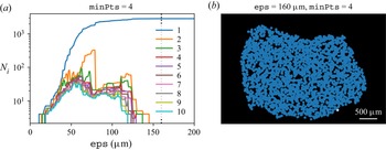
Since a continuous velocity field might not always be available, we now consider the case where one only has discrete trajectory data for a small subset of cells. We simulate such a scenario by randomly initializing 6000 cells and advecting them under the PIV-derived velocity field. Using this single set of trajectory data, we utilize our approach for detecting hyperbolic LCSs described in § 2.1.2 with  $\delta = 100 \ \mathrm {\mu } \mathrm {m}$. The resulting discrete forward FTLE is shown at initial time in figure 8(d) and the discrete backward FTLE is shown at final time in figure 8(f); both agree well with their continuous counterparts. Most importantly, the ridges delineating the repelling and attracting LCSs are still clearly visible, despite the sparsity of the discrete dataset. Such agreement validates the applicability of our methodology for the computation of hyperbolic LCSs to sparse and noisy real-life experimental datasets. In Appendix G, we also apply our algorithm for the detection of elliptic LCSs to the same dataset, returning one large elliptic LCS enclosing most of the cells. This highlights the complementary nature of our methods to detect both types of LCSs, since there does not always exist well-defined LCSs of each type in any system.
3.4. Gulf of Mexico
In our last example, we analyse the trajectories of a set of 152 acoustically tracked isobaric floats in the Gulf of Mexico (Hamilton et al. Reference Hamilton, Bower, Furey, Leben and Pérez-Brunius2016). The floats were ballasted for a depth of  $1500\ \mathrm {m}$ and deployed over a two-year period starting in 2011, with each float recording its position over a duration varying between a week and 1.5 years. Based on a probabilistic Markov chain analysis (Froyland, Stuart & van Sebille Reference Froyland, Stuart and van Sebille2014) of these trajectories, Miron et al. (Reference Miron, Beron-Vera, Olascoaga, Froyland, Pérez-Brunius and Sheinbaum2019) found that the deep circulation dynamics consist of two weakly interacting provinces of near-equal area, in each of which drifters had a residence time of 3.5 to4.5 years.
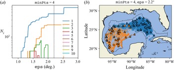
We now search for elliptic LCSs in this dataset, following our method described in § 2.2. From the 152 float trajectories, we first select 35 that persist over the same time, here chosen to be 610 days. Using the pairwise distance definition (2.10), we then apply the DBSCAN algorithm with  $\texttt {minPts} = 4$ since the trajectories are two-dimensional. Figure 9(a) shows the number
 $N_i$ of particles in each of the ten largest resulting groups. We discard groups 3 to 10 (and beyond) since they repeatedly appear and disappear as
 $\texttt {eps}$ varies. The size of the remaining two physically meaningful groups remains constant for
 $\texttt {eps}$ in the range
 $2^\circ$ to
 $2.5^\circ$. We thus pick
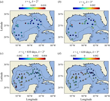
 $\texttt {eps} = 2.2^\circ$ and plot the corresponding clusters in figure 9(b) by colouring the trajectories (lines) and the initial (triangles) and final (circles) positions of the floats according to their cluster membership. We recover the two equally sized regions of coherent motion that were identified in Miron et al. (Reference Miron, Beron-Vera, Olascoaga, Froyland, Pérez-Brunius and Sheinbaum2019). Notably, this was achieved at much lower human effort and computational cost, since the latter study requires the construction of a spatial grid over which the matrix of transition probabilities is calculated. By contrast, our approach is meshless, straightforward to implement and takes less than a second of computational time in this particular case. In Appendix H, we also apply our algorithm for the detection of hyperbolic LCSs to the same dataset, seemingly uncovering a repelling LCS separating the two regions of coherent motion. However, the computed FTLE field is very sensitive to the value of
 $\delta$, which illustrates that extreme sparsity of the data can make the detection of hyperbolic LCSs challenging.
Elliptic LCSs in the deep Gulf of Mexico, using trajectories produced over 610 days by 35 acoustically tracked isobaric floats at a depth of  $1500 \ \mathrm {m}$. (a) Number
 $N_i$ of floats in each of the ten largest groups identified by the DBSCAN algorithm as a function of
 $\texttt {eps}$, for
 $\texttt {minPts} = 3$. (b) The two coherent groups identified by DBSCAN for
 $\texttt {eps} = 2.2^\circ$ are shown in blue and orange, in terms of the initial (triangles) and final (circles) positions of the floats as well as their trajectories (lines). The black dotted line indicates the
 $1500 \ \mathrm {m}$ isobath.

4. Conclusions
We have introduced objective computational techniques for detecting hyperbolic and elliptic LCSs in complex flow systems based solely on knowledge of sparse and noisy particle trajectories. These techniques were validated using two benchmark problems defined by analytical velocity fields: the two-dimensional Bickley jet and the chaotic three-dimensional ABC flow. For hyperbolic LCSs, our technique exhibited better robustness to measurement noise than other leading methods. For elliptic LCSs, our methodology identified structures more consistently than competing methods, at a lower computational cost and without arbitrary parameter choices. We then applied our techniques to two experimental datasets: the global flow of cells in a developing chicken embryo and the trajectories of ballasted floats in the Gulf of Mexico, identifying the key LCSs organizing these complex flows.
In the past, the complexity, computational requirements, sensitivity or lack of publicly available codes of most existing techniques for LCSs detection have prevented their broad use in engineering, physical and biological problems. To this end, this study is accompanied by a simple, lightweight and user-friendly Python code that implements our methods on any dataset of particle trajectories.
The present work opens the door to several avenues of future research. In our approach to detect hyperbolic structures, the least-squares problem (2.5) gives equal weights to all particle pairs contained within a ball of a given radius around the point of interest. Weighting each pair according to its distance from the point of interest or the number of similarly oriented pairs may improve the accuracy of the fit, similar to the Voronoi-based weighting proposed in Lekien & Ross (Reference Lekien and Ross2010). Likewise, the clustering results of DBSCAN are heavily dependent on the definition (2.10) of the distance between two trajectories, which currently measures the time average of the instantaneous pairwise distance. Taking inspiration from Schlueter-Kuck & Dabiri (Reference Schlueter-Kuck and Dabiri2017a), one can use metrics such as the temporal standard deviation of the pairwise distance or alternative synchronization measures. Finally, we envisage extending our methods to account for incomplete and or newly added trajectories. Examples include ocean drifters that break down or temporarily lose GPS tracking, and dividing or dying cells.
Supplementary movies
Supplementary movies are available at https://doi.org/10.1017/jfm.2022.652.
Acknowledgements
We thank the reviewers for comments that led to many improvements. We acknowledge M. Chuai and C.J. Weijer for providing the chicken embryo dataset.
Funding
M.S. acknowledges partial support from the Schmidt Science Fellowship and the Postdoc Mobility Fellowship from the Swiss National Foundation. L.M. thanks the NSF-Simons Center for Mathematical and Statistical Analysis of Biology Award 1764269, NIH 1R01HD097068, the Simons Foundation and the Henri Seydoux Fund for partial support.
Code accessibility
Python codes implementing the methods described are shared in an online repository at https://github.com/smowlavi/CoherentStructures and can readily be applied to any experimental or computational dataset of particle trajectories.
Declaration of interests
The authors declare no conflict of interest.
Appendix A. Solution of the least-squares problem
Here, we describe how to solve the least-squares problem defined by (2.5), which includes Tikhonov regularization (Kaipio & Somersalo Reference Kaipio and Somersalo2006). With the matrices  $\boldsymbol{\mathsf{X}}, \boldsymbol{\mathsf{Y}} \in \mathbb {R}^{d \times m}$ introduced in (2.8), one can rewrite (2.5) in matrix form as follows:
 \begin{equation} \tilde{\boldsymbol{\nabla}} \boldsymbol{F}_{t_0}^t(\boldsymbol{x}_0^i) = \arg \min_{\boldsymbol{\mathsf{A}}} J(\boldsymbol{\mathsf{A}}) \equiv \arg \min_{\boldsymbol{\mathsf{A}}} \,\frac{1}{M} \left\Vert \boldsymbol{\mathsf{A}} \boldsymbol{\mathsf{X}} - \boldsymbol{\mathsf{Y}} \right\Vert_F^2 + \beta \Vert \boldsymbol{\mathsf{A}} - \boldsymbol{\mathsf{I}} \Vert_F^2. \end{equation}
Due to the convexity of the objective function  $J(\boldsymbol{\mathsf{A}})$, its global minimum is obtained when its gradient with respect to
 $\boldsymbol{\mathsf{A}}$ vanishes. To calculate the gradient, we utilize the definition of the Frobenius norm to expand each term in the objective function
 $J(\boldsymbol{\mathsf{A}})$ as
 $$\begin{gather} \left\Vert \boldsymbol{\mathsf{A}} \boldsymbol{\mathsf{X}} - \boldsymbol{\mathsf{Y}} \right\Vert_F^2 = \text{tr}[ (\boldsymbol{\mathsf{A}} \boldsymbol{\mathsf{X}} - \boldsymbol{\mathsf{Y}})^{\mathrm{T}} (\boldsymbol{\mathsf{A}} \boldsymbol{\mathsf{X}} - \boldsymbol{\mathsf{Y}}) ] = \text{tr}[ \boldsymbol{\mathsf{X}}^{\mathrm{T}} \boldsymbol{\mathsf{A}}^{\mathrm{T}} \boldsymbol{\mathsf{A}} \boldsymbol{\mathsf{X}} - \boldsymbol{\mathsf{X}}^{\mathrm{T}} \boldsymbol{\mathsf{A}}^{\mathrm{T}} \boldsymbol{\mathsf{Y}} - \boldsymbol{\mathsf{Y}}^{\mathrm{T}} \boldsymbol{\mathsf{A}} \boldsymbol{\mathsf{X}} + \boldsymbol{\mathsf{Y}}^{\mathrm{T}} \boldsymbol{\mathsf{Y}} ], \end{gather}$$
 $$\begin{gather}\left\Vert \boldsymbol{\mathsf{A}} - \boldsymbol{\mathsf{I}} \right\Vert_F^2 = \text{tr}[ (\boldsymbol{\mathsf{A}} - \boldsymbol{\mathsf{I}})^{\mathrm{T}} (\boldsymbol{\mathsf{A}} - \boldsymbol{\mathsf{I}}) ] = \text{tr}[ \boldsymbol{\mathsf{A}}^{\mathrm{T}} \boldsymbol{\mathsf{A}} - \boldsymbol{\mathsf{A}}^{\mathrm{T}} - \boldsymbol{\mathsf{A}} + \boldsymbol{\mathsf{I}} ]. \end{gather}$$
Applying standard matrix calculus identities, the gradient of the objective function  $J(\boldsymbol{\mathsf{A}})$ with respect to matrix
 $\boldsymbol{\mathsf{A}}$ is then given by
 \begin{equation} \frac{\partial J(\boldsymbol{\mathsf{A}})}{\partial \boldsymbol{\mathsf{A}}} = \frac{2}{M} \boldsymbol{\mathsf{A}} \boldsymbol{\mathsf{X}} \boldsymbol{\mathsf{X}}^{\mathrm{T}} - \frac{2}{M} \boldsymbol{\mathsf{A}} \boldsymbol{\mathsf{Y}} \boldsymbol{\mathsf{X}}^{\mathrm{T}} + 2 \lambda \boldsymbol{\mathsf{A}} - 2 \beta \boldsymbol{\mathsf{I}}. \end{equation}
Setting the above derivative to zero and solving for  $\boldsymbol{\mathsf{A}}$, one finally obtains the solution given in (2.6).
Appendix B. Identifying spurious groups in the Bickley jet and ABC flow
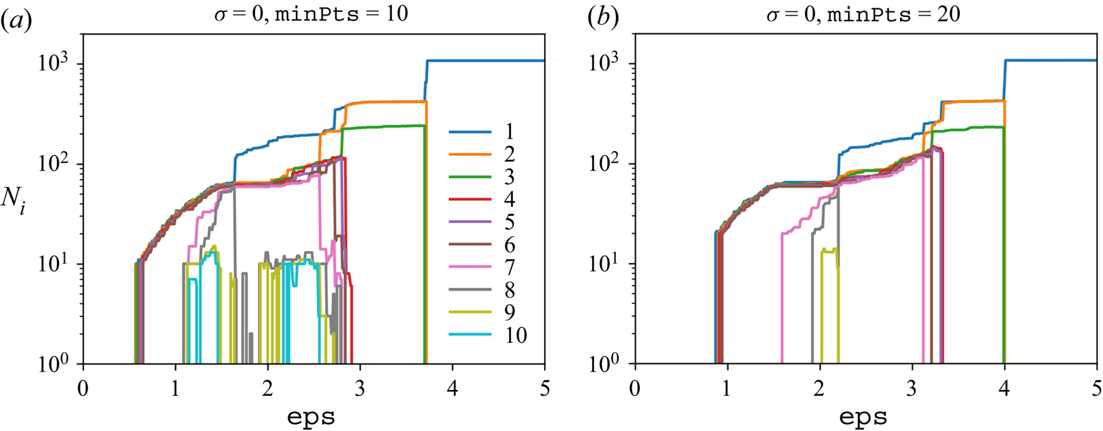
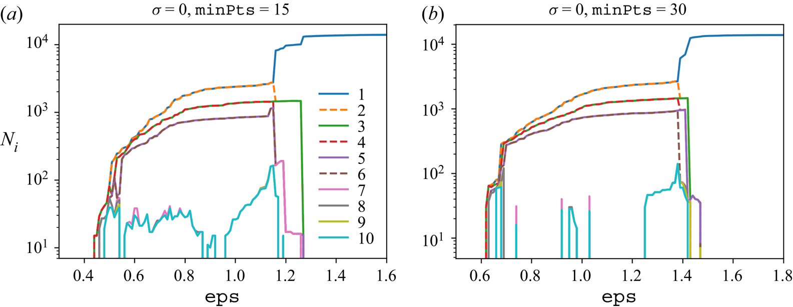
In this appendix, we repeat the calculation performed in figures 5(a) and 7(a) for the Bickley jet and ABC flow, respectively, but with higher values of  $\texttt {minPts}$. The goal is to identify, among the coherent groups returned by DBSCAN, those that are not physically meaningful. As described in the parameter selection strategy in § 2.2, such spurious groups are characterized by a large sensitivity of their size to the parameter
 $\texttt {eps}$ or by their complete disappearance in many ranges of values of
 $\texttt {eps}$. The latter phenomenon most often occurs for values of
 $\texttt {minPts}$ larger than the recommended
 $\texttt {minPts}$ equal to twice the number of dimensions.
Beginning with the Bickley jet, we consider the same dataset and  $\sigma = 0$ as in figure 5(a) and plot in figure 10 the number
 $N_i$ of particles in the ten largest groups identified by DBSCAN versus
 $\texttt {eps}$, this time using larger values of
 $\texttt {minPts} = 10$ and
 $20$. We observe that groups 8 to 10 repeatedly appear and disappear under small changes of
 $\texttt {eps}$ for
 $\texttt {minPts} = 10$, and are completely gone in most of the
 $\texttt {eps}$ range for
 $\texttt {minPts} = 20$. This confirms that groups 8 and above are spurious. For the ABC flow, we consider the same dataset and
 $\sigma = 0$ as in figure 7(a) and plot in figure 11 the number
 $N_i$ of particles in the ten largest groups identified by DBSCAN versus
 $\texttt {eps}$, this time using larger values of
 $\texttt {minPts} = 15$ and
 $30$. Here again, we observe that groups 7 to 10 repeatedly appear and disappear under small changes of
 $\texttt {eps}$, which confirms that they are spurious.
Same as figure 5(a) but for ( $a$)
 $\texttt {minPts} = 10$ and (
 $b$)
 $\texttt {minPts} = 20$.

Same as figure 7(a) but for (a)  $\texttt {minPts} = 15$ and (b)
 $\texttt {minPts} = 30$.

Appendix C. Apparent outliers in the Bickley jet
We analyse the trajectories of two particles labelled as belonging to the green cluster in figure 5(e) for the Bickley jet with  $\texttt {minPts} = 10$,
 $\texttt {eps} = 5$ and
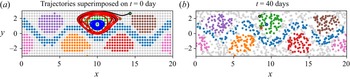
 $\sigma = 0$, despite being located away from the rest of the cluster at initial time. The red and black lines in figure 12(a) show the trajectories of these two particles with their initial positions indicated by circles, together with the trajectory, in blue, of a third particle that is initially located near the middle of the green cluster. We also display the entire clusters obtained in figure 5(e) at
 $t = 0$ day. The trajectories reveal that the two apparent outlier particles in fact rapidly converge towards the green cluster, justifying their membership in the latter. Figure 12(b) depicts the final positions at
 $t = 40$ days of these two outliers as the red and black circles, together with the final position of the particle that started near the middle of the green cluster as the blue circle. The entire clusters are also displayed at
 $t = 40$ days, showing that all three particles are located in the interior of the green cluster. Thus, the DBSCAN algorithm is correct in assigning these two apparent outliers to the green cluster. A similar analysis shows that the two apparent outliers of the orange cluster rapidly converge towards the latter, justifying their labelling as well.
Fate of two seemingly outlier particles in the green Bickley jet cluster obtained in figure 5(e) using  $\texttt {minPts} = 10$,
 $\texttt {eps} = 5$ and
 $\sigma = 0$. (a) Initial positions (red and black circles) and trajectories (red and black lines) of these two apparent outliers superimposed with the position at
 $t = 0$ day of the entire clusters obtained in figure 5(e). We also show the trajectory (blue line) of a particle that is initially located near the middle of the green cluster. (b) Final positions (red and black circles) of the same two apparent outliers superimposed with the clusters displayed at
 $t = 40$ days, together with the final position (blue circle) of the particle that started near the middle of the green cluster.

Appendix D. Bickley jet and ABC flow results with increased data sparsity
In this appendix, we demonstrate the ability of our methods to handle various levels of sparsity by revisiting the Bickley jet and ABC flow examples investigated in §§ 3.1 and 3.2, but using fewer particles this time.
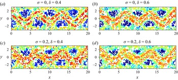
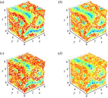
Starting with hyperbolic LCSs, we compute the trajectories of a set of randomly initialized particles and we apply white Gaussian noise of standard deviation  $\sigma$ to each trajectory, as we did before. We use 2000 particles for the Bickley jet and 30 000 particles for the ABC flow. Figures 13 and 14 show the discrete FTLE fields in the Bickley jet and ABC flow, respectively, computed using the least-squares technique described in § 2.1.2 for different values of
 $\sigma$ and the neighbourhood radius
 $\delta$. Although the ridges of the FTLE field are coarser than in the presence of more data, we can still delineate the two ridges that separate the meandering jet from the vortices in the Bickley jet, and the ridges between the coherent vortices in the ABC flow. As we have observed before, increasing the parameter
 $\delta$ leads to cleaner ridges, especially in the presence of measurement noise.
Hyperbolic repelling LCSs in the Bickley jet with fewer particles. Discrete FTLE field computed over the time window  $t \in [0,40]$ using 2000 particles with (a)
 $\sigma = 0$,
 $\delta = 0.4$, (b)
 $\sigma = 0$,
 $\delta = 0.6$, (c)
 $\sigma = 0.2$,
 $\delta = 0.4$ and (d)
 $\sigma = 0.2$,
 $\delta = 0.6$. Here,
 $\sigma$ refers to the standard deviation of observation noise, and
 $\delta$ is the neighbourhood radius used in the least-squares fit of the flow map gradient. The colourbar is the same as in figure 4.

Hyperbolic repelling LCSs in the ABC flow with fewer particles. Discrete FTLE field computed over the time window  $t \in [0,20]$ using 30 000 particles with (a)
 $\sigma = 0$,
 $\delta = 0.3$, (b)
 $\sigma = 0$,
 $\delta = 0.4$, (c)
 $\sigma = 0.2$,
 $\delta = 0.3$ and (d)
 $\sigma = 0.2$,
 $\delta = 0.4$. Here,
 $\sigma$ refers to the standard deviation of observation noise, and
 $\delta$ is the neighbourhood radius used in the least-squares fit of the flow map gradient. The colourbar is the same as in figure 6.

Next, we apply the clustering approach described in § 2.2 to compute elliptic LCSs using a set of particle trajectories initialized on a grid and polluted by white Gaussian noise of standard deviation  $\sigma$. We use 480 particles for the Bickley jet and 3375 particles for the ABC flow. As before, we account for the periodicity of the domain – in the
 $x$ direction for the Bickley jet and all three directions for the ABC flow – when calculating the pairwise Euclidean distance entering (2.10). We then apply the DBSCAN algorithm, using
 $\texttt {minPts}$ equal to twice the dimensionality of the dataset and various values of
 $\texttt {eps}$. For the Bickley jet and ABC flow, respectively, figures 15(a,b) and 16(a,b) show the number
 $N_i$ of particles in each of the ten largest resulting groups as a function of
 $\texttt {eps}$, for two values of the noise
 $\sigma$. Despite the fewer number of particles, these plots are remarkably similar to their counterparts in figures 5(a,b) and 7(a,b). Finally, we discard spurious groups and select
 $\texttt {eps}$ in a range where the size of the remaining, physically meaningful groups remains stable. The corresponding clusters are plotted in figures 15(c,d) and 16(c,d) for the Bickley jet and ABC flow, respectively, and they identify the same coherent structures that were obtained in §§ 3.1 and 3.2. We note that the similarity between the membership curves in figures 15(a,b), 16(a,b) and their counterparts in figures 5(a,b), 7(a,b) demonstrates the robustness of our parameter selection methodology to the simultaneous presence of noise and sparsity in the data.
Elliptic LCSs in the Bickley jet with fewer particles. (a,b) Number  $N_i$ of particles in each of the ten largest groups identified by the DBSCAN algorithm as a function of the parameter
 $\texttt {eps}$ for
 $\texttt {minPts} = 7$. The data consist of 480 particle trajectories advected over
 $t \in [0,40]$ and artificially polluted by observation noise of standard deviation (a)
 $\sigma = 0$ and (b)
 $\sigma = 2$. (c,d) Coherent groups identified by DBSCAN for (c)
 $\sigma = 0$ and (d)
 $\sigma = 2$, using the value of
 $\texttt {eps}$ shown as the dotted line in (a,b).

Elliptic LCSs in the ABC flow with fewer particles. (a,b) Number  $N_i$ of particles in each of the ten largest groups identified by the DBSCAN algorithm as a function of the parameter
 $\texttt {eps}$ for
 $\texttt {minPts} = 20$. The data consist of 3375 particle trajectories advected over
 $t \in [0,20]$ and artificially polluted by observation noise of standard deviation (a)
 $\sigma = 0$ and (b)
 $\sigma = 2$. (c,d) Coherent groups identified by DBSCAN for (c)
 $\sigma = 0$ and (d)
 $\sigma = 2$, using the value of
 $\texttt {eps}$ shown as the dotted line in (a,b).

Appendix E. Bickley jet and ABC flow results with three alternative techniques
In this appendix, we compute hyperbolic LCSs in the Bickley jet and ABC flow using three alternative techniques for sparse datasets: the original least-squares approach for computing the FTLE on unstructured grids from Lekien & Ross (Reference Lekien and Ross2010) which forms the basis for our technique, the fitted ellipse approach for computing the FTLE from Rypina et al. (Reference Rypina, Getscher, Pratt and Mourre2021) and the trajectory stretching exponent  $\overline {\mathrm {TSE}}$ introduced in Haller et al. (Reference Haller, Aksamit and Encinas-Bartos2021). We note that the first two techniques require a set of neighbours for every particle at which the FTLE is computed, which we obtain from a Delaunay triangulation of the initial particle positions.
Beginning with the Bickley jet, we employ the same dataset of 6000 randomly initialized particles and the same noise values  $\sigma$ employed in figure 4 to compute the FTLE using the techniques from Lekien & Ross (Reference Lekien and Ross2010) and Rypina et al. (Reference Rypina, Getscher, Pratt and Mourre2021), and the
 $\overline {\mathrm {TSE}}$ from Haller et al. (Reference Haller, Aksamit and Encinas-Bartos2021) over the time window
 $t \in [0,40]$. The results are displayed in figure 17 and can be compared with ours in figure 4. In the absence of noise, the discrete FTLE from Lekien & Ross (Reference Lekien and Ross2010) and Rypina et al. (Reference Rypina, Getscher, Pratt and Mourre2021) give comparable results to our method with
 $\delta = 0.3$. With noise, however, the results degrade since these techniques were not designed to cope with noisy data. On the other hand, our method benefits from the presence of the extra parameter
 $\delta$, which helps to smooth out pollution from noise when it is increased – indeed, our results in the presence of noise exhibit much clearer and continuous ridges when
 $\delta = 0.5$. As for the
 $\overline {\mathrm {TSE}}$ from Haller et al. (Reference Haller, Aksamit and Encinas-Bartos2021), we observe in the absence of noise that its particle-wise values display a first jump across the jet boundaries (from blue to green) and a second jump inside the jet itself (from green to red). It is therefore challenging to define an unequivocal criterion based on the
 $\overline {\mathrm {TSE}}$ for identifying the two hyperbolic repelling LCSs that delineate the jet boundaries. In addition, these jumps are not robust to noise since evaluating the
 $\overline {\mathrm {TSE}}$ requires knowledge of particle velocities, whose calculation amplifies the noise polluting the particle positions.
Hyperbolic repelling LCSs in the Bickley jet, computed using alternative approaches with the same dataset as in figure 4. (a,b) Discrete FTLE from Lekien & Ross (Reference Lekien and Ross2010), (c,d) discrete FTLE from Rypina et al. (Reference Rypina, Getscher, Pratt and Mourre2021) and (e,f)  $\overline {\mathrm {TSE}}$ from Haller et al. (Reference Haller, Aksamit and Encinas-Bartos2021) with (a,c,e)
 $\sigma = 0$ and (b,d,f)
 $\sigma = 0.2$. Here,
 $\sigma$ refers to the standard deviation of observation noise.

For the ABC flow, we employ the same dataset of 120 000 randomly initialized particles and the same noise values  $\sigma$ employed in figure 6 to compute the FTLE from Lekien & Ross (Reference Lekien and Ross2010), the FTLE from Rypina et al. (Reference Rypina, Getscher, Pratt and Mourre2021) and the
 $\overline {\mathrm {TSE}}$ from Haller et al. (Reference Haller, Aksamit and Encinas-Bartos2021) over the time window
 $t \in [0,20]$. The results are displayed in figure 18 and can be compared with ours in figure 6. Once again, without noise the discrete FTLE from Lekien & Ross (Reference Lekien and Ross2010) and Rypina et al. (Reference Rypina, Getscher, Pratt and Mourre2021) give similar results to using our method with
 $\delta = 0.2$. In the presence of noise, however, increasing
 $\delta$ to 0.3 in our method leads to much cleaner FTLE ridges than obtained with these two approaches. As for the
 $\overline {\mathrm {TSE}}$, it is observed like before to be less robust to noise than our technique.
Hyperbolic repelling LCSs in the ABC flow, computed using alternative approaches with the same dataset as in figure 6. (a,b) Discrete FTLE from Lekien & Ross (Reference Lekien and Ross2010), (c,d) discrete FTLE from Rypina et al. (Reference Rypina, Getscher, Pratt and Mourre2021) and (e,f)  $\overline {\mathrm {TSE}}$ from Haller et al. (Reference Haller, Aksamit and Encinas-Bartos2021) with (a,c,e)
 $\sigma = 0$ and (b,d,f)
 $\sigma = 0.2$. Here,
 $\sigma$ refers to the standard deviation of observation noise.

Appendix F. Relative dispersion in the Bickley jet and the ABC flow
In this appendix, we revisit the Bickley jet and ABC flow datasets through the lens of relative dispersion, a metric used in oceanography to analyse advection of passive tracers (Provenzale Reference Provenzale1999). The relative dispersion  $D^2$ over a time window
 $[t_0,t]$ is defined as the mean square distance at time
 $t$ between particle pairs that are initially separated by a small distance
 $d_0$. This average is usually taken over particle pairs seeded in different locations of the same flow, meaning that the relative dispersion is a global quantity in which local features of non-homogeneous flows are lost. Although the proper way to remedy this issue is to take an ensemble average over particle pairs released at the same location in different realizations of the flow, such realizations are often not available when only one experiment is recorded. In such a case, Haller & Yuan (Reference Haller and Yuan2000) introduce the relative dispersion density field
 $d^2$, defined at every initial particle location as the square distance at time
 $t$ between said particle and another one that was initially a small distance
 $d_0$ away. When applying this metric to the Bickley jet and ABC flow, we instead consider the closest neighbour since the random distribution of initial particle positions precludes the existence of a neighbour initially located exactly
 $d_0$ away.
In the next paragraph, we see that the  $d^2$ field is very noisy as its calculation relies on a single pair of particles. Thus, we introduce an improved metric that we call generalized relative dispersion density
 $d_g^2$, defined at every initial particle location as the average of the square distance at time
 $t$ between all particle pairs initially contained within a ball of radius
 $\delta$. In a sense, this new metric blends the definitions of
 $D^2$ and
 $d^2$ by replacing the global average over all particle pairs in
 $D^2$ by a local average over particle pairs in the proximity of a given particle.This metric is similar in spirit to the approximate FTLE introduced in § 2.1.2, since both are calculated based on the same set of particle pairs contained in a local ball of radius
 $\delta$. We therefore expect the two techniques to yield similar results, which we see below.
Beginning with the Bickley jet, we employ the same dataset of 6000 randomly initialized particles and the same noise values  $\sigma$ employed in figure 4 to compute the relative dispersion density
 $d^2$ and its generalized counterpart
 $d_g^2$ over the time window
 $t \in [0,40]$. For
 $d_g^2$, we also utilize the same
 $\delta$ values as in figure 4. The results are displayed in figure 19 and can be compared with ours in figure 4. The
 $d^2$ field is very noisy since it is computed at every point from single particle pairs. Although its highest values are located along the hyperbolic LCSs, these values do not form a continuous ridge as in the case of the FTLE field computed with our method. This can be explained by the fact that the relative dispersion density is sensitive to both the initial location and the initial orientation of the particle pair. Indeed, among particle pairs located on a hyperbolic LCS, only those approximately perpendicular to it will yield a high value of
 $d^2$. On the other hand, the
 $d_g^2$ field that we have introduced shows a semi-continuous ridge of high values along the hyperbolic LCSs, since averaging over multiple particle pairs erases the dependence of
 $d_g^2$ on the orientation of individual pairs. As expected,
 $d_g^2$ shares visual similarities with the FTLE approximated using our least-squares approach. Our FTLE-based method nonetheless leads to a delineated continuous ridge of high values along the hyperbolic LCSs, since the underlying flow map gradient inherently takes into account the orientation of every particle pair.
Relative dispersion metrics in the Bickley jet, computed using the same dataset as in figure 4. (a,b) Square root of the relative dispersion density (RDD)  $d^2$ and (c,d) square root of the generalized relative dispersion density (GRRD)
 $d_g^2$ with (a,c)
 $\sigma = 0$ and (b,d)
 $\sigma = 0.2$. Here,
 $\sigma$ refers to the standard deviation of observation noise.

For the ABC flow, we employ the same dataset of 120 000 randomly initialized particles and the same noise values  $\sigma$ employed in figure 6 to compute the relative dispersion density
 $d^2$ and its generalized counterpart
 $d_g^2$ over the time window
 $t \in [0,20]$. For
 $d_g^2$, we also utilize the same
 $\delta$ values as in figure 6. The results are displayed in figure 20 and can be compared with ours in figure 6. The observations are identical to those for the Bickley jet. The
 $d^2$ field is very noisy and does not have a continuous ridge of large values along the hyperbolic LCSs. On the other hand, the
 $d_g^2$ field that we have introduced displays a semi-continuous ridge of high values along the hyperbolic LCSs and shares visual similarities with the FTLE approximated using our least-squares approach. However, there are many locations along the hyperbolic LCSs where the ridge of high
 $d_g^2$ values cuts off. This issue is not present in our least-squares approximation of the FTLE, which therefore remains the best method for identifying hyperbolic LCSs.
Relative dispersion metrics in the ABC flow, computed using the same dataset as in figure 6. (a,b) Square root of the relative dispersion density (RDD)  $d^2$ and (c,d) square root of the generalized relative dispersion density (GRDD)
 $d_g^2$ with (a,c)
 $\sigma = 0$ and (b,d)
 $\sigma = 0.2$. Here,
 $\sigma$ refers to the standard deviation of observation noise.

Appendix G. Elliptic LCSs in the chicken embryo
We apply our algorithm for the detection of elliptic LCSs to the flow of cells in the developing chicken embryo from § 3.3. We consider the same sparse set of 6000 simulated cell trajectories used in figure 8(d,f) and follow the procedure described in § 2.2 using  $\texttt {minPts} = 4$, since the data are two-dimensional. Figure 21(a) shows the number
 $N_i$ of particles in each of the ten largest resulting groups as a function of
 $\texttt {eps}$. According to our parameter selection strategy, groups 2 and above are all spurious since their size is highly sensitive to
 $\texttt {eps}$ and they disappear for larger values of
 $\texttt {minPts}$. Thus, we are left with a single physically meaningful group, consisting of the blue particles in figure 21(b). This example shows that there might not always exist distinct elliptic LCSs in an arbitrary dataset.
Elliptic LCSs in the flow of cells belonging to a developing chick embryo (Rozbicki et al. Reference Rozbicki, Chuai, Karjalainen, Song, Sang, Martin, Knölker, MacDonald and Weijer2015), using 6000 random uniformly distributed particles at initial time and advected with the flow of cells. (a) Number  $N_i$ of floats in each of the ten largest groups identified by the DBSCAN algorithm as a function of
 $\texttt {eps}$, for
 $\texttt {minPts} = 4$. (b) The DBSCAN algorithm only identifies one coherent group shown in blue, along with a few noise particles.

Appendix H. Hyperbolic LCSs in the Gulf of Mexico
We apply our algorithm for the detection of hyperbolic LCSs to the ocean float trajectories from § 3.4. We consider the same set of 35 trajectories that overlap during 610 days and follow the technique described in § 2.1.2 using different values for  $\delta$. The resulting discrete forward FTLE is shown at initial time in figure 22(a,b) and the discrete backward FTLE is shown at final time in figure 22(c,d). The results suggest the presence of a repelling LCS at initial time separating the two regions of coherent motion identified by the elliptic LCSs in figure 9(b). However, both the forward FTLE and backward FTLE values are very sensitive to the value of
 $\delta$ due to the extreme sparsity of the data, which renders an accurate assessment of hyperbolic LCSs in this system impossible. We note that Getscher (Reference Getscher2021) applied the least-squares FTLE technique from Lekien & Ross (Reference Lekien and Ross2010) to a set of 135 drifter trajectories from the SPLASH experiment. Although these drifters were released in a nearly gridded pattern, the resulting FTLE field became very noisy as soon as the time window of interest exceeded 3 days, highlighting the inherent challenges in computing FTLE fields using such sparse data.
Hyperbolic LCSs in the deep Gulf of Mexico, using trajectories produced over 610 days by 35 acoustically tracked isobaric floats at a depth of  $1500 \ \mathrm {m}$. (a,b) Discrete forward-time FTLE field at initial time and (c,d) discrete backward-time FTLE field at final time, computed using (a,c)
 $\delta = 2^\circ$ and (b,d)
 $\delta = 3^\circ$. The FTLE values are in
 ${\rm day}^{-1}$.