1. Introduction
In processes which involve production of fluids from a subsurface porous layer through a well, interventions occur whereby from time to time two fluids are pumped in sequence into the porous rock from the well. One example of this occurs when reservoir engineers inject a chemical treatment to consolidate the oil-bearing sands (Paraskeva et al. Reference Paraskeva, Charalambous, Stokka, Klepetsanis, Koutsoukos, Read, Ostvold and Payatakes2000) or introduce an agent that inhibits the precipitation of salts in the event of any mixing between geologic and injected water (Woods Reference Woods2015). After the chemical treatment is injected into the rock from the well, post-treatment fluid is typically used to clean-up the well and as a result the finite volume of treatment fluid is displaced by the post-treatment fluid, and forms an annulus some distance beyond the well. Talaghat, Esmaeilzadeh & Mowla (Reference Talaghat, Esmaeilzadeh and Mowla2009) describe how it is difficult to obtain a uniform front of the injected chemical owing to the time-constraint of injecting the treatment as quickly as possible, since the well is unproductive during such interventions. Any break-up or fingering of the treatment fluid might lead to regions in which the treatment fluid is unable to form a competent bond designed to prevent sand production.
The challenge for such injection arises where adverse viscosity ratios are present. As well as two-phase flow effects, the interfaces are subject to the possible development of viscous fingering. In this study, in order to build fundamental understanding of such coupled interface flows, we analyse the stability of an idealised flow involving two unstable interfaces spreading radially from a central source in a Hele-Shaw geometry. We use the analysis to select an optimum viscosity for the treatment fluid so as to prevent any instability during the injection process while maximising the injection rate.
Paterson (Reference Paterson1981) pioneered the study of the single-interface radial viscous instability in a Hele-Shaw geometry, determining the linear growth rates of the different azimuthal modes. This analysis has been developed in a number of directions. For example, Miranda & Widom (Reference Miranda and Widom1998) investigated weakly nonlinear tip-splitting phenomena, whilst Parisio et al. (Reference Parisio, Moraes, Miranda and Widom2001) explored viscous fingering on the surface of a sphere. More recently, there has been interest in the control of such phenomena. Cardoso & Woods (Reference Cardoso and Woods1995) explained how fingering could be prevented by keeping the interface linearly stable at low flow rates. Li et al. (Reference Li, Lowengrub, Fontana and Palffy-Muhoray2009) developed a nonlinear analysis and a technique to control the final shape of the interface. In the context of Hele-Shaw flow, the possibility of control through varying the gap width has been explored (Al-Housseiny & Stone Reference Al-Housseiny and Stone2013; Dias & Miranda Reference Dias and Miranda2013).
The two-interface problem was first introduced by Nayfeh (Reference Nayfeh1972) and later developed by Cardoso & Woods (Reference Cardoso and Woods1995) who performed a theoretical and experimental dual-interface analysis in the special case in which the inner fluid is highly viscous. With a stable trailing interface and an unstable leading interface, they modelled the formation of drops from the annulus of intermediate fluid. However, in the present problem of well treatment, both interfaces are likely to be unstable. Recently, Gin & Daripa (Reference Gin and Daripa2015) examined the growth rates of instabilities in a dual-interface system as a function of the viscosity of the three fluids in the system. In that analysis less attention was placed on the conditions for overall stability; however, this is relevant for the injection of treatment fluid followed by a volume of post-treatment clean-up fluid, and forms the focus of the present work. Our ultimate aim is to select the viscosity of the intermediate (treatment) fluid so as to minimise the overall injection time for both the treatment fluid and the subsequent post-treatment fluid, whilst ensuring overall stability of the system. We assume that the original reservoir (outer) fluid is more viscous than the post-treatment (inner) fluid, and that the treatment fluid is of intermediate viscosity. For simplicity, we assume that the treatment fluid is immiscible with both the reservoir fluid and the post-treatment fluid, so that there is interfacial tension at both interfaces. In this regard, we note that if two fluids are only weakly soluble and hence only partially miscible, this can also lead to an effective interfacial stress (Korteweg Reference Korteweg1901; Pojman et al. Reference Pojman, Whitmore, Liria, Liveri, Lombardo, Marszalek, Parker and Zoltowski2006).
First, in § 2 we analyse the linear stability of a single interface as a reference calculation and identify that there is a maximum flow rate below which all modes are stable. We relate this maximum flow rate to the viscosity of the displacing fluid. In § 3 we explore the dual-interface system and determine conditions for both absolute stability of the lowest modes of the system, and also dynamic stability of all modes through control of the flow rate. In § 4 we use these results to find the optimal choice of the viscosity of the treatment fluid so as to minimise the injection time.
2. Single-interface stability: treatment injection phase
2.1. Formulation
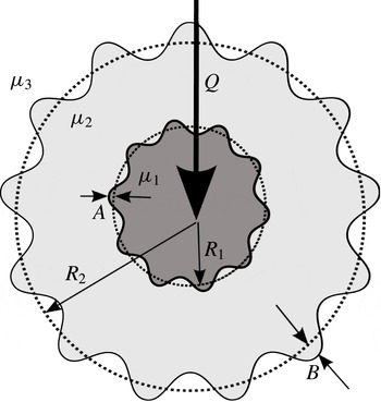
The flow configuration is shown in figure 1. In this section, we consider the stability of the leading interface alone. Paterson (Reference Paterson1981) showed that the linear growth of perturbations of the form
 $$\begin{eqnarray}b_{n}=B_{n}(t)\text{e}^{\text{i}n{\it\theta}}\end{eqnarray}$$
during radial displacement of a single interface is given by
 $$\begin{eqnarray}\frac{1}{B_{n}}\frac{\partial B_{n}}{\partial t}=\frac{Qc_{23}n}{2{\rm\pi}R_{2}^{2}}-\frac{Q}{2{\rm\pi}R_{2}^{2}}-\frac{{\it\kappa}Tn(n^{2}-1)}{R_{2}^{3}({\it\mu}_{2}+{\it\mu}_{3})}.\end{eqnarray}$$
In (2.2),
 $B_{n}$
is the amplitude of azimuthal mode
 $n$
,
 $Q$
is the volumetric flow rate per unit depth,
 $R_{2}$
is the radial position of the interface,
 ${\it\mu}_{i}$
is the viscosity of species
 $i$
,
 ${\it\kappa}$
is the permeability,
 $T$
is the interfacial tension, the viscosity contrast
 $c_{ij}=({\it\mu}_{j}-{\it\mu}_{i})/({\it\mu}_{j}+{\it\mu}_{i})$
, the treatment fluid is labelled 2 and the displaced reservoir fluid is labelled 3. The first term on the right-hand side represents viscous destabilisation and the second and third terms represent the stabilising effects of stretching of the interface and interfacial tension respectively.
Dual-interface variable definitions. The reservoir fluid (fluid 3) and post-treatment fluid (fluid 1) are separated by an annulus of treatment fluid (fluid 2). The leading and trailing interfacial base states are at radii
 $R_{2}$
and
 $R_{1}$
respectively, with perturbation amplitudes
 $B_{n}(t)$
and
 $A_{n}(t)$
.

2.2. Absolute stability of mode
 $n$

For each mode
 $n$
, equating the viscous destabilisation term with the stretching term gives the maximum viscosity contrast for which the interface is stable for any flow rate, at all radii,
 $$\begin{eqnarray}c_{23}\leqslant 1/n.\end{eqnarray}$$
We refer to this as absolute stability. We envisage that the treatment fluid is of intermediate viscosity between the reservoir fluid and the post-treatment fluid and so introduce a parameter
 $P$
, the ratio of the viscosity difference between the treatment fluid and the reservoir fluid, compared to the viscosity difference between the post-treatment fluid (labelled 1) and the reservoir fluid. We also introduce a viscosity ratio between the post-treatment fluid and reservoir fluid
 $V$
. They are respectively given by
 $$\begin{eqnarray}P=\frac{{\it\mu}_{3}-{\it\mu}_{2}}{{\it\mu}_{3}-{\it\mu}_{1}},\quad V=\frac{{\it\mu}_{1}}{{\it\mu}_{3}}.\end{eqnarray}$$
Hence, we can rewrite (2.3) in terms of
 $P$
and
 $V$
:
 $$\begin{eqnarray}P\leqslant \frac{2}{(1-V)(n+1)}.\end{eqnarray}$$
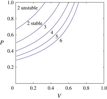
The values of
 $P$
for absolute stability of mode
 $n$
are shown in figure 2 for
 $n=2,\ldots ,6$
. As
 $V$
increases or
 $P$
decreases higher modes become absolutely stable. Both regions are labelled for mode 2, otherwise each region is labelled with the highest mode that is absolutely stable.
Variation of the maximum value of
 $P$
at which the labelled mode,
 $n=2,\ldots ,6$
, becomes absolutely stable as a function of
 $V$
. For a given mode
 $n$
, then for values of
 $P$
smaller than this maximum, all modes
 $n^{\prime }$
such that
 $n^{\prime }<n$
are absolutely stable.

2.3. Dynamic stability
If the viscosity contrast is higher than that given by (2.3), the viscous destabilisation term must be equated with the interfacial tension and stretching terms in order to control mode
 $n$
. This yields a maximum flow rate
 $Q_{n}(R_{2})$
for which mode
 $n$
is stable at a finite radius,
 $R_{2}$
:
 $$\begin{eqnarray}Q_{n}(R_{2})=\frac{1}{R_{2}}\frac{2{\rm\pi}{\it\kappa}Tn(n^{2}-1)}{(n({\it\mu}_{3}-{\it\mu}_{2})-({\it\mu}_{3}+{\it\mu}_{2}))}.\end{eqnarray}$$
It is convenient to scale
 $Q_{n}(R_{2})$
by
 $Q_{\mathit{ref}}$
, the flow rate at which mode 2 would go unstable at the well radius (
 $R_{w}$
) if the reservoir fluid were displaced by an inviscid species. Hence
 $$\begin{eqnarray}\displaystyle & \displaystyle Q_{\mathit{ref}}=\frac{12{\rm\pi}{\it\kappa}T}{R_{w}{\it\mu}_{3}}, & \displaystyle\end{eqnarray}$$
 $$\begin{eqnarray}\displaystyle & \displaystyle R_{2}^{\ast }=\frac{R_{2}}{R_{w}}, & \displaystyle\end{eqnarray}$$
 $$\begin{eqnarray}\displaystyle & \displaystyle t^{\ast }=t\frac{Q_{\mathit{ref}}}{{\rm\pi}R_{w}^{2}}, & \displaystyle\end{eqnarray}$$
 $$\begin{eqnarray}\displaystyle & \displaystyle Q_{n}^{\ast }(R_{2})=\frac{Q_{n}(R_{2})}{Q_{\mathit{ref}}}, & \displaystyle\end{eqnarray}$$
 $$\begin{eqnarray}\displaystyle & \displaystyle {\it\Gamma}(n)=Q_{n}^{\ast }(R_{2}^{\ast })R_{2}^{\ast }=\frac{n(n^{2}-1)}{6\left((n+1)P(1-V)-2\right)}. & \displaystyle\end{eqnarray}$$
 ${\it\Gamma}(n)$
,
 ${\it\Gamma}(n_{\mathit{min}})$
say, identifies the highest dimensionless flow rate such that the interface is stable to all such azimuthal modes (2.1). Higher modes are stabilised by interfacial tension, and lower modes by stretching. As an approximation for large
 $n_{\mathit{min}}$
, we can find the solution
 $n=n_{\mathit{min}}$
by finding a solution of
 $\text{d}{\it\Gamma}/\text{d}n=0$
. This is given by the real, positive root of the equation
 $$\begin{eqnarray}n^{3}(2P(1-V))-n^{2}(6-3P(1-V))-(P(V-1)+2)=0.\end{eqnarray}$$
This provides a good approximation for large
 $n$
, but is inexact since
 $n$
is discrete. Note that there is only one real positive root of (2.12) if
 $P(1-V)<2$
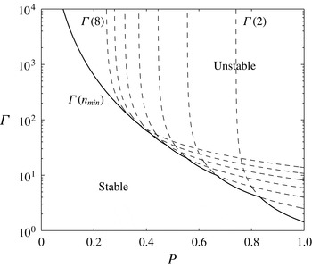
, which is always true if the treatment fluid is of intermediate viscosity. In figure 3 we plot
 ${\it\Gamma}(n)$
for modes
 $n=2$
–8 (dotted lines) and
 ${\it\Gamma}(n_{\mathit{min}})$
(solid line) as a function of
 $P$
. The figure illustrates how for smaller viscosity jumps,
 $P$
, the interface remains stable at larger flow rates
 ${\it\Gamma}$
(2.11).
Stability diagram for a radial displacement flow with
 $V=0.1$
, showing the highest value of
 ${\it\Gamma}(n)=Q_{n}^{\ast }(R_{2}^{\ast })R_{2}^{\ast }$
for which the flow is stable to perturbations of mode
 $n$
(dashed lines) plotted as a function of the ratio of the viscosity difference between the reservoir fluid and the treatment fluid, and the viscosity difference between the post-treatment fluid and the reservoir fluid. Solid line represents the locus of stability for all modes
 ${\it\Gamma}(n_{\mathit{min}})$
as a function of
 $P$
. If a more viscous displacing fluid is used, higher flow rates are permitted.

2.4. Single-interface control
The time
 $t$
taken for the interface to advance to radius
 $R_{2}(t)$
starting with radius
 $R_{2}(0)=1$
when injected at the highest dimensionless stable flow rate
 ${\it\Gamma}(n_{\mathit{min}})/R_{2}(t)$
is
 $$\begin{eqnarray}t=\int _{1}^{R_{2}}\frac{2{R^{\prime }}_{2}^{2}}{{\it\Gamma}(n_{\mathit{min}})}\text{d}R_{2}^{\prime }=\frac{2}{3}\frac{(R_{2}^{3}-1)}{{\it\Gamma}(n_{\mathit{min}})}\end{eqnarray}$$
and this implies that the dynamically stable flow rate,
 $Q(R_{2})$
, is
 $$\begin{eqnarray}Q(R_{2})=Q_{n=n_{\mathit{min}}}(R_{2})=\frac{{\it\Gamma}(n_{\mathit{min}})}{\left(1+\frac{3}{2}{\it\Gamma}(n_{\mathit{min}})t\right)^{1/3}}.\end{eqnarray}$$
In the limit
 $t\gg 1$
 $$\begin{eqnarray}Q(R_{2})={\it\Gamma}(n_{\mathit{min}})^{2/3}\left({\textstyle \frac{3}{2}}t\right)^{-1/3}.\end{eqnarray}$$
This generalises the result of Cardoso & Woods (Reference Cardoso and Woods1995) (their equation (5.2)) who analysed the limiting case of a large viscosity contrast in which only mode 2 needs to be considered.
This calculation identifies the maximum flow rate to ensure stability during the period in which there is one interface. During this phase it is desired to make
 ${\it\Gamma}(n_{\mathit{min}})$
as large as possible, which can be achieved by making the injected fluid more viscous (such that
 $c_{23}\rightarrow 0$
). However, by doing so the subsequent clean-up phase (in which post-treatment fluid displaces the chemical treatment) tends to develop an unstable interface. The destabilisation of the trailing interface in an annular system could lead to the break-up of the annulus of treatment fluid. Hence, we seek an optimum viscosity to minimise the time the well is out of production for given volumes of treatment chemical and post-treatment fluid. In order to inform this selection of viscosity we model the stability of a two-interface system in § 3.
3. Dual-interface stability: post-treatment fluid injection phase
3.1. Formulation
In this section we calculate the maximum flow rate for stability for a three fluid system, in which there are two interfaces at positions
 $R_{1}(t)+a({\it\theta},t)$
and
 $R_{2}(t)+b({\it\theta},t)$
, where
 $a$
and
 $b$
are small perturbations to the shape of the interface. In general we can express the perturbations of the interfaces in the form of a power series:
 $$\begin{eqnarray}\left.\begin{array}{@{}c@{}}\displaystyle a({\it\theta},t)={\it\Sigma}_{n=1}^{n\rightarrow \infty }A_{n}(t)\text{e}^{\text{i}n{\it\theta}},\\ \displaystyle b({\it\theta},t)={\it\Sigma}_{n=1}^{n\rightarrow \infty }B_{n}(t)\text{e}^{\text{i}n{\it\theta}}.\end{array}\right\}\end{eqnarray}$$
A schematic of the variables used in the calculation is shown in figure 1. The velocity potential
 ${\it\phi}$
is related to velocity
 $\boldsymbol{v}$
and the pressure
 $p$
by Darcy’s law for flow in porous media:
 $$\begin{eqnarray}\boldsymbol{v}=-\frac{{\it\kappa}}{{\it\mu}}\boldsymbol{{\rm\nabla}}p=-\boldsymbol{{\rm\nabla}}{\it\phi},\end{eqnarray}$$
and the flow is incompressible hence the velocity potentials obey Laplace’s equation,
 ${\rm\nabla}^{2}{\it\phi}=0$
. The solution is assumed to be comprised of a steady solution
 ${\it\phi}_{j}^{0}=-Q/(2{\rm\pi})\,\text{ln}\,r+c_{j}$
and, for mode
 $n$
, a first-order perturbation
 ${\it\phi}_{j}^{1}={\it\Sigma}_{n=1}^{n\rightarrow \infty }{\it\phi}_{j,n}^{1}(r,t)\text{e}^{\text{i}n{\it\theta}}$
where for mode
 $n$
, the linearised perturbation has radial structure
 ${\it\phi}_{j,n}^{1}$
given by Laplace’s equation (for
 $j=1,2,3$
):
 $$\begin{eqnarray}\left.\begin{array}{@{}c@{}}\displaystyle {\it\phi}_{1,n}^{1}={\it\alpha}_{n}(t)\left(\frac{r}{R_{1}}\right)^{n},\\ \displaystyle {\it\phi}_{2,n}^{1}={\it\beta}_{n}(t)\left(\frac{r}{R_{1}}\right)^{-n}+{\it\gamma}_{n}(t)\left(\frac{r}{R_{2}}\right)^{n},\\ \displaystyle {\it\phi}_{3,n}^{1}={\it\epsilon}_{n}(t)\left(\frac{r}{R_{2}}\right)^{-n}.\end{array}\right\}\end{eqnarray}$$
Owing to the orthogonality of the modes, it follows that for each mode
 $n$
at the trailing interface,
 $R_{1}$
, the continuity of velocity and the jump in pressure owing to interfacial tension are given by (Cardoso & Woods Reference Cardoso and Woods1995)
 $$\begin{eqnarray}\displaystyle & \displaystyle \frac{\partial v_{1}^{0}}{\partial r}A_{n}+v_{1,n}^{1}=\frac{\partial v_{2}^{0}}{\partial r}A_{n}+v_{2,n}^{1}=\frac{\text{d}A_{n}}{\text{d}t}, & \displaystyle\end{eqnarray}$$
 $$\begin{eqnarray}\displaystyle & \displaystyle \frac{\partial }{\partial r}\left(\frac{{\it\phi}_{1}^{0}{\it\mu}_{1}}{{\it\kappa}}\right)A_{n}+\frac{{\it\phi}_{1,n}^{1}{\it\mu}_{1}}{{\it\kappa}}=\frac{\partial }{\partial r}\left(\frac{{\it\phi}_{2}^{0}{\it\mu}_{2}}{{\it\kappa}}\right)A_{n}+\frac{{\it\phi}_{2,n}^{1}{\it\mu}_{2}}{{\it\kappa}}-\frac{T(1-n^{2})}{R_{1}^{2}}A_{n}, & \displaystyle\end{eqnarray}$$
 $v_{j,n}^{1}=-(\partial /\partial r){\it\phi}_{j,n}^{1}$
. Similar conditions may be written for the leading interface at
 $R_{2}$
. Substituting the velocity potentials (3.3) into the boundary conditions (3.4), (3.5) and eliminating
 ${\it\alpha}_{n}(t)$
,
 ${\it\beta}_{n}(t)$
,
 ${\it\gamma}_{n}(t)$
and
 ${\it\epsilon}_{n}(t)$
yields the following set of coupled ordinary differential equations (ODEs) for each mode
 $n$
:
 $$\begin{eqnarray}\hspace{-12.0pt}\left.\begin{array}{@{}l@{}}\displaystyle \frac{\text{d}A_{n}}{\text{d}t}=\underbrace{f_{1}\left(\frac{Q(n-f_{1}^{-1})}{2{\rm\pi}R_{1}^{2}}-\frac{T{\it\kappa}n(n^{2}-1)}{R_{1}^{3}({\it\mu}_{2}-{\it\mu}_{1})}\right)A_{n}}_{\text{(i)}}+\underbrace{f_{2}\left(\frac{Qn}{2{\rm\pi}R_{2}^{2}}-\frac{T{\it\kappa}n(n^{2}-1)}{R_{2}^{3}({\it\mu}_{3}-{\it\mu}_{2})}\right)B_{n}}_{\text{(ii)}},\\ \displaystyle \frac{\text{d}B_{n}}{\text{d}t}=\underbrace{f_{3}\left(\frac{Qn}{2{\rm\pi}R_{1}^{2}}-\frac{T{\it\kappa}n(n^{2}-1)}{R_{1}^{3}({\it\mu}_{2}-{\it\mu}_{1})}\right)A_{n}}_{\text{(iii)}}+\underbrace{f_{4}\left(\frac{Q(n-f_{4}^{-1})}{2{\rm\pi}R_{2}^{2}}-\frac{T{\it\kappa}n(n^{2}-1)}{R_{2}^{3}({\it\mu}_{3}-{\it\mu}_{2})}\right)B_{n}}_{\text{(iv)}},\\ \displaystyle \text{where}\\ \hspace{72.0pt}\displaystyle f_{1}={\displaystyle \frac{c_{12}(1-c_{23}\hat{R}^{2n})}{1+c_{12}c_{23}\hat{R}^{2n}}},\quad \displaystyle f_{2}={\displaystyle \frac{c_{23}(1+c_{12})\hat{R}^{n+1}}{1+c_{12}c_{23}\hat{R}^{2n}}},\\ \hspace{72.0pt}\displaystyle f_{3}={\displaystyle \frac{c_{12}(1-c_{23})\hat{R}^{n-1}}{1+c_{12}c_{23}\hat{R}^{2n}}},\quad \displaystyle f_{4}={\displaystyle \frac{c_{23}(1+c_{12}\hat{R}^{2n})}{1+c_{12}c_{23}\hat{R}^{2n}}},\\ \hspace{156.0pt}\displaystyle \hat{R}=\frac{R_{1}}{R_{2}}.\end{array}\right\}\end{eqnarray}$$
The terms labelled (i) and (iv) on the right-hand sides of (3.6) describe local behaviour in which we can recognise terms for viscous destabilisation, stretching of the interface and interfacial tension (cf. (2.2)). The terms labelled (ii) and (iii) couple the two interfaces and in the limit of a thick annulus (
 $\hat{R}\rightarrow 0$
) they become weak, leaving two separate single interfaces. The coupled ODEs can be written in matrix form:
 $$\begin{eqnarray}\frac{\text{d}}{\text{d}t}\binom{A_{n}}{B_{n}}=\unicode[STIX]{x1D648}\binom{A_{n}}{B_{n}}.\end{eqnarray}$$
The growth rates of the system (
 ${\it\lambda}^{+},{\it\lambda}^{-}$
) are the eigenvalues of
 $\unicode[STIX]{x1D648}$
. In the limit of a thin annulus (
 $\hat{R}\rightarrow 1$
;
 $R_{1}=R_{2}$
) the growth rates have the asymptotic form
 $$\begin{eqnarray}\left.\begin{array}{@{}c@{}}\displaystyle {\it\lambda}^{+}=\frac{Qc_{13}n}{2{\rm\pi}R_{2}^{2}}-\frac{Q}{2{\rm\pi}R_{2}^{2}}-\frac{2{\it\kappa}Tn(n^{2}-1)}{R_{2}^{3}}\frac{1}{{\it\mu}_{1}+{\it\mu}_{3}},\\ \displaystyle {\it\lambda}^{-}=-\frac{Q}{2{\rm\pi}R_{2}^{2}}.\end{array}\right\}\end{eqnarray}$$
In (3.8) the largest growth rate is that which would occur with species 1 displacing species 3 (no annulus; cf. (2.2)), but with twice the individual interfacial tension. In the limit of a stable inner interface (
 ${\it\mu}_{1}\gg {\it\mu}_{2},{\it\mu}_{3}$
) the result matches that given by Cardoso & Woods (Reference Cardoso and Woods1995). These asymptotic limits were also derived by Gin & Daripa (Reference Gin and Daripa2015).
To understand the controls on the onset of instability, and hence determine the critical flow rate to ensure stability, it is of interest to study the nature of the instabilities as the three controlling parameters
 $\hat{R}$
,
 $V$
and
 $P$
vary.
3.2. Absolute stability of mode
$n$

The single-interface stability problem reveals the fascinating result that there is a viscosity contrast below which a mode is stable at all flow rates and radii (absolute stability), based on the balance between the stretching of the interface due to the radial spreading and the viscous destabilisation. We can draw from that result to provide insight into the two-interface problem.
For small values of
 $\hat{R}$
, we expect the two interfaces to be largely decoupled. We expect that as
 $P$
increases the outer interface becomes progressively more unstable. To assess this transition in more detail, it is useful to consider how the condition for absolute stability depends on the viscosity change between the treatment and reservoir fluids,
 $P$
, and also the ratio between the post-treatment and reservoir fluid viscosity
 $V$
. We can then generalize these results for
 $\hat{R}=\mathit{O}(1)$
where coupling between the interfaces becomes significant.
Absolute stability results from balancing viscous destabilisation with stretching, and in the dual system this is done by setting
 $\text{Det}(\unicode[STIX]{x1D648})=0$
with
 $T=0$
. This yields
 $$\begin{eqnarray}c_{12}c_{23}(1-\hat{R}^{2n})n^{2}-(c_{12}+c_{23})n+1+c_{12}c_{23}\hat{R}^{2n}=0.\end{eqnarray}$$
In the limit
 $\hat{R}\rightarrow 0$
, (3.9) gives the condition for absolute stability of mode
 $n$
from § 2.2 for two separate single interfaces
 $$\begin{eqnarray}\left.\begin{array}{@{}l@{}}\displaystyle c_{12}\leqslant \frac{1}{n},\\ \displaystyle c_{23}\leqslant \frac{1}{n}.\end{array}\right\}\end{eqnarray}$$
These conditions are combined by writing them in terms of
 $P$
, giving the condition for absolute stability for mode
 $n$
:
 $$\begin{eqnarray}\frac{1-{\displaystyle \frac{n+1}{n-1}}V}{1-V}\leqslant P\leqslant \frac{2}{(1-V)(n+1)}.\end{eqnarray}$$
Below the lower bound the trailing interface is locally not absolutely stable, and likewise above the upper bound the leading interface is not. Equating these conditions gives a critical
 $V$
below which neither interface, in isolation, can be absolutely stable:
 $$\begin{eqnarray}V_{\mathit{lower}}(n)=\left(\frac{n-1}{n+1}\right)^{2}.\end{eqnarray}$$
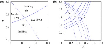
In figure 4(a) we show the upper
 $P$
bound of the absolutely stable region as a solid line (familiar from § 2.2) and the lower bound
 $P$
as a dashed line for mode 2 as a function of
 $V$
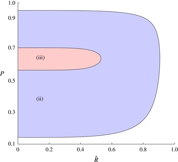
. The system is only absolutely stable in region (ii). Elsewhere, viscous destabilisation on one or both interfaces is possible and can only be stabilised by controlling flow rate. In figure 4(b) we extend this to higher modes by indicating which modes (
 $n^{\prime }\leqslant n$
) are absolutely stable in each domain. This figure is important since it illustrates how, at the onset of instability, the lowest modes in the system may not be unstable at all, depending on the parameters
 $P$
and
 $V$
. To determine which mode will be unstable first, the effect of interfacial tension must be considered (see § 3.3).
The non-dimensional difference in viscosity across the leading interface,
 $P$
, at which the trailing (dashed) and leading (solid) interfaces become absolutely stable to the given mode as a function of the bounding viscosity ratio,
 $V$
for the limit
 $\hat{R}\rightarrow 0$
. In (a) we show which interface is absolutely stable for mode 2. In regions (i) and (iii) the leading or trailing interface alone is respectively absolutely stable, whereas in region (ii) both interfaces are absolutely stable and in region (iv) both interfaces impose a flow rate limitation for stability. In (b) we show how this extends to higher modes.

As fluid continues to be supplied to the system, the inner radius grows and
 $\hat{R}$
increases. This leads to a progressively increasing level of coupling between the leading and trailing interfaces. In the case
 $V>V_{\mathit{lower}}(n=2)$
, we identified values of
 $P$
for which mode 2 becomes absolutely stable with
 $\hat{R}\ll 1$
; as
 $\hat{R}$
increases, we expect that the coupling will cause these bounding values of
 $P$
to converge, and eventually that there is a value of
 $\hat{R}$
for which there is no longer a region of absolute stability for mode 2. The bounding values of
 $P$
can be found by solving (3.9) at chosen values of
 $V,\hat{R}$
and
 $n$
. We illustrate this trend in figure 5 in which we show how the bounding values of
 $P$
vary with
 $\hat{R}$
for mode 2 where
 $V=0.3$
. The boundary for mode 3 is also plotted and is contained within that of mode 2. In this case, there are no regions of absolute stability for mode 4 since
 $0.3<V_{\mathit{lower}}(n=4)$
.
The critical values of the non-dimensional leading viscosity jump,
 $P$
, for absolute stability as a function of
 $\hat{R}$
for
 $V=0.3$
. In regions (ii) and (iii) modes 2 and 3 are absolutely stable respectively. As time and hence
 $\hat{R}$
increase, the annulus thins and these lines converge. As such, absolute stability is transient for modes 2 and 3 for this value of
 $V$
.

In the limit of a thin annulus,
 $\hat{R}\rightarrow 1$
, (3.9) has the asymptotic form
 $$\begin{eqnarray}c_{13}\leqslant \frac{1}{n}.\end{eqnarray}$$
This condition can be obtained by considering a single interface with post-treatment fluid displacing reservoir fluid directly (see § 2.2). It can also be written as a function of
 $V$
:
 $$\begin{eqnarray}V_{\mathit{upper}}(n)=\frac{n-1}{n+1}.\end{eqnarray}$$
Equation (3.14) shows that in the case
 $V>1/3$
, the instability that would result from post-treatment fluid directly displacing the reservoir fluid is only unstable to higher modes,
 $n\geqslant 3$
, and so the two-interface problem is also only unstable to these higher modes. In this case, depending on the value of
 $P$
we expect that the most unstable mode could correspond to much higher values of
 $n$
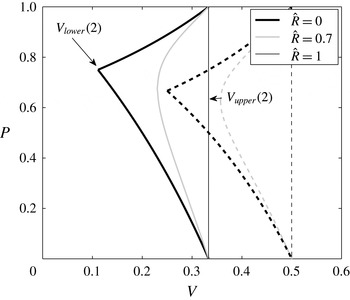
. Figure 6 shows how the absolutely stable region of figure 4 evolves as
 $\hat{R}$
increases for mode 2 (solid lines) and mode 3 (broken lines). As
 $\hat{R}$
increases, the bounds tend towards a vertical line at
 $V_{\mathit{upper}}(n)$
. The system is only absolutely stable if an interface between the post-treatment and reservoir fluid is absolutely stable. The cusp at
 $V_{\mathit{lower}}(n)$
for mode 3 is larger than the cusp for mode 2, as expected from figure 5.
The critical values of the non-dimensional difference in viscosity across the leading interface,
 $P$
, at which the dual-interface system is absolutely stable as a function of
 $V$
for modes 2 (solid lines) and 3 (broken lines) for three values of
 $\hat{R}$
. The
 $\hat{R}=0$
curves can be recognised from figure 4 with cusps at
 $V_{\mathit{lower}}(n)$
. As
 $\hat{R}$
increases, the annulus thins and the stability tends to that of a single interface in a system in which the post-treatment fluid displaces the reservoir fluid, with a vertical boundary at
 $V_{\mathit{upper}}(n)$
.

We have found that if
 $V_{\mathit{lower}}(n)<V<V_{\mathit{upper}}(n)$
there are solutions of (3.9) that are transient absolutely stable bounds of
 $P$
, i.e. initially mode
 $n$
can be absolutely stable but later in the flow interfacial tension must be considered for dynamic stability. Below this range there is no absolute stability and above it mode
 $n$
remains absolutely stable at all radii. If mode
 $n$
is absolutely stable, we must consider the dynamic stability of a higher mode to find the maximum flow rate for the system’s stability.
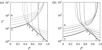
Variation of the maximum flow rate,
 ${\it\Gamma}=QR_{2}$
, for stability of the system to all modes (thick solid line) as a function of the non-dimensional leading viscosity jump,
 $P$
, for
 $V=0.1$
and for (a)
 $\hat{R}=0.1$
, (b)
 $\hat{R}=0.5$
. Also shown are a series of thin lines on which
 $\text{Det}(\unicode[STIX]{x1D648})=0$
for each of modes
 $2,\ldots ,6$
. In (a), for
 $n>2$
, there are two dashed lines for each mode: one of these lines has relatively small values of
 ${\it\Gamma}$
for small
 $P$
and
 ${\it\Gamma}$
then increases monotonically with
 $P$
, whilst the other has relatively small values of
 ${\it\Gamma}$
for large
 $P$
and
 ${\it\Gamma}$
then decreases monotonically with
 $P$
. The point of intersection of these two solution branches corresponds to the point
 $\text{Det}(\unicode[STIX]{x1D648})=0$
and
 $\text{Tr}(\unicode[STIX]{x1D648})=0$
. However, for
 $n=2$
, there are two non-intersecting lines for which
 $\text{Det}(\unicode[STIX]{x1D648})=0$
and these are shown as solid thin lines. The lower branch corresponds to the maximum value of
 ${\it\Gamma}$
for which all perturbations of mode 2 are stable, while the upper branch corresponds to the minimum value of
 ${\it\Gamma}$
for which all perturbations of mode 2 are unstable. In (b), we show solutions for
 $\text{Det}(\unicode[STIX]{x1D648})=0$
for modes
 $n=2,\ldots ,5$
as thin solid lines, and for each such mode, there is a lower branch on which
 $\text{Tr}(\unicode[STIX]{x1D648})<0$
and an upper branch on which
 $\text{Tr}(\unicode[STIX]{x1D648})>0$
, and these branches do not intersect. Note, however, that owing to the finite vertical scale, the upper branch of mode 2 does not appear in the graph. Also shown are two dashed thin lines, corresponding to
 $\text{Det}(\unicode[STIX]{x1D648})=0$
for mode 6. The value of
 ${\it\Gamma}$
on these two dashed lines increases and decrease monotonically with
 $P$
, respectively, and their point of intersection again corresponds to the point
 $\text{Det}(\unicode[STIX]{x1D648})=0$
and
 $\text{Tr}(\unicode[STIX]{x1D648})=0$
.

3.3. Dynamic stability
In general, the condition for stability is found by balancing the viscous destabilisation with the stretching and interfacial tension terms to ensure
 ${\it\lambda}^{+}=0$
, since if either growth rate were positive the perturbations would grow. The eigenvalues are given by
 $$\begin{eqnarray}{\it\lambda}^{\pm }=\frac{\text{Tr}(\unicode[STIX]{x1D648})}{2}\pm \sqrt{\left(\frac{\text{Tr}(\unicode[STIX]{x1D648})^{2}}{4}-\text{Det}(\unicode[STIX]{x1D648})\right)}.\end{eqnarray}$$
It can be seen from (3.15) that if
 $\text{Tr}(\unicode[STIX]{x1D648})\leqslant 0$
and
 $\text{Det}(\unicode[STIX]{x1D648})=0$
, then
 ${\it\lambda}^{+}=0$
and
 ${\it\lambda}^{-}<0$
. If we solve the relation
 $\text{Det}(\unicode[STIX]{x1D648})=0$
we find two solutions for
 $Q_{n}(R)$
, but only one of these is in a region where
 $\text{Tr}(\unicode[STIX]{x1D648})\leqslant 0$
and therefore represents stability. To illustrate the evolution of the stability of the different modes as the fluids invade the pore space and the trailing front catches up with the leading front, in figure 7 we present the maximum value of
 ${\it\Gamma}=QR_{2}$
(thick line) below which the system is stable for the cases
 $\hat{R}=0.1$
and
 $\hat{R}=0.5$
where
 $V=0.1$
.
Figure 7(a) corresponds to small
 $\hat{R}$
at early times in the injection process when the two interfaces are far apart. In this limit then, to leading order, the stability of each interface may be approximated by the local stability of that interface (3.6). In this case, the thick line showing the maximum flow rate for stability is approximately given by the mode 2 stability bound of the trailing interface for small
 $P$
, but as
 $P$
increases, this intersects the mode 6 stability bound of the leading interface. As
 $P$
continues to increase, the critical flow rate for stability is given by successively lower modes, until coinciding, approximately, with the mode 2 stability of the leading interface.
In this limit of small
 $\hat{R}$
, since the interfaces are far apart, the stability curves
 $\text{Det}(\unicode[STIX]{x1D648})=0$
for the higher modes are well approximated by the stability curves for that mode on each of the two interfaces individually, and the effects of the coupling between the interfaces are small. Indeed, in figure 7(a) for all the higher modes,
 $n>2$
, with
 $\hat{R}=0.1$
there is a common point at which
 $\text{Det}(\unicode[STIX]{x1D648})=0$
and
 $\text{Tr}(\unicode[STIX]{x1D648})=0$
which connects the solutions
 $\text{Det}(\unicode[STIX]{x1D648})=0$
with
 $\text{Tr}(\unicode[STIX]{x1D648})<0$
and the solutions
 $\text{Det}(\unicode[STIX]{x1D648})=0$
with
 $\text{Tr}(\unicode[STIX]{x1D648})>0$
. For a given mode,
 $n>2$
, as we move across the point
 $\text{Det}(\unicode[STIX]{x1D648})=0$
and
 $\text{Tr}(\unicode[STIX]{x1D648})=0$
, on the line
 $\text{Det}(\unicode[STIX]{x1D648})=0$
we can interpret this point as corresponding to that at which the stability of the mode changes from being dominated by one interface to the other. The main exception to this for
 $\hat{R}=0.1$
is for the lowest mode, mode 2 (solid thin line). Here, it is seen that for mode 2 the solution of the relation
 $\text{Det}(\unicode[STIX]{x1D648})=0$
does not intersect the solution
 $\text{Tr}(\unicode[STIX]{x1D648})=0$
; instead for mode 2 two non-intersecting branches of the solution
 $\text{Det}(\unicode[STIX]{x1D648})=0$
may be seen.
 $\text{Tr}(\unicode[STIX]{x1D648})<0$
on the lower branch and
 $\text{Tr}(\unicode[STIX]{x1D648})>0$
on the upper branch. The coupling between the interfaces leads to a loss of the special solution,
 $\text{Det}(\unicode[STIX]{x1D648})=0$
and
 $\text{Tr}(\unicode[STIX]{x1D648})=0$
, for the lowest mode, mode 2. Instead there is a smooth adjustment along the line
 $\text{Det}(\unicode[STIX]{x1D648})=0$
from the solution dominated by the leading interface when
 $P\approx 1$
to the trailing interface when
 $P\approx 0$
.
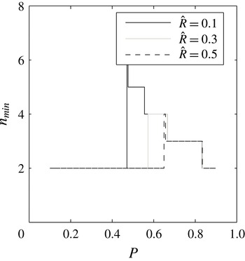
The mode that requires the lowest flow rate to remain stable (
 $n_{\mathit{min}}$
) as a function of
 $P$
for
 $V=0.1$
and
 $\hat{R}=0.1,0.3,0.5$
. As
 $\hat{R}$
increases coupling causes lower modes to impose the strictest limit on flow rate.

However, as more fluid is injected and the trailing interface catches up with the leading interface,
 $\hat{R}=0.5$
(figure 7
b), then the distance between the interfaces becomes smaller and so some of the higher modes, notably modes 3–5, in the case
 $\hat{R}=0.5$
, also become highly coupled. As a result, for each of these modes there is no longer a solution
 $\text{Det}(\unicode[STIX]{x1D648})=0$
with
 $\text{Tr}(\unicode[STIX]{x1D648})=0$
. Again, two independent solution branches for
 $\text{Det}(\unicode[STIX]{x1D648})=0$
emerge for each of these modes. On the lower branch in
 $(P,{\it\Gamma})$
space,
 $\text{Tr}(\unicode[STIX]{x1D648})<0$
, and on a separate higher solution branch
 $\text{Det}(\unicode[STIX]{x1D648})=0$
we have
 $\text{Tr}(\unicode[STIX]{x1D648})>0$
. Now the lower solution branch determines the maximum flow rate,
 ${\it\Gamma}$
, for which that mode is stable to all perturbations.
In figure 7(b), the thick line again shows the overall stability boundary for all modes in terms of the maximum values of
 ${\it\Gamma}$
for which the modes are stable, as a function of
 $P$
. For small
 $P$
, the stability threshold is determined by mode 2. However, for this larger value of
 $\hat{R}$
,
 $\hat{R}=0.5$
, figure 7(b) shows that, as
 $P$
increases, this first intersects the stability boundary for the higher modes with the mode 4 stability curve. With further increases in the value of
 $P$
, this overall stability threshold is given by mode 3 and then back to mode 2 at very large
 $P$
.
It is also seen from the figure that higher modes only become unstable for large values of
 ${\it\Gamma}$
and so are not rate-limiting in determining the maximum flow rate for stability. Indeed, in figure 8 we illustrate the most unstable mode for three representative values of
 $\hat{R}$
as a function of
 $P$
. In accord with the form of figure 7, it is seen that as the value of
 $P$
increases from close to 0, the most unstable mode jumps from mode 2 to mode 6 when
 $P$
has value of order 0.45, but then as
 $P$
continues to increase this most unstable mode gradually falls again to mode 2.
This figure, in conjunction with figure 7, demonstrates how lower modes impose stricter limitations on the maximum stable flow rate as
 $\hat{R}$
increases.
Our analysis has identified that, for small
 $\hat{R}$
, it is possible that the system is only unstable to higher modes depending on
 $P$
and
 $V$
. If
 $V>V_{\mathit{lower}}$
(3.12), all modes
 $n^{\prime }<n$
can be absolutely stable for a range of
 $P$
. As
 $\hat{R}$
increases, these lower modes also become progressively unstable. If
 $V>V_{\mathit{upper}}(n)$
(3.14), all modes
 $n^{\prime }<n$
are stable for all
 $P$
and
 $\hat{R}$
. As fluid continues to be injected, the interfacial tension, which is the mechanism ensuring stability, becomes progressively weaker. As a result, in order to ensure the stability of the system, the injection rate should progressively decrease. Depending on the values of
 $P$
and
 $V$
, the mode imposing the strictest limit on flow rate to maintain stability may become lower with increasing
 $\hat{R}$
. Owing to the transition in this strictest-limit mode with the injection of a finite volume of fluid, the minimum time required for injection whilst maintaining stability depends on the choice of
 $P$
.
(a) The maximum stable
 ${\it\Gamma}=QR_{2}$
as a function of
 $P$
for a series of increasing
 $R_{2}$
where
 $V=0.1$
. The post-treatment fluid is injected at
 $R_{2}=5$
. As such, for
 $1\leqslant R_{2}\leqslant 5$
the stability of the system is bounded by the single-interface analysis (broken line). Subsequently, the stability of the trailing interface must be considered and the stability is bounded by the dual-interface analysis (solid lines). (b) The variation of maximum
 $Q$
for stability with
 $R_{2}$
for the cases A, B and C in (a).

4. Control strategy
The aim of this section is to identify the optimal value of viscosity of chemical treatment to minimise injection time. This will depend on the viscosity ratio of the post-treatment fluid and reservoir fluid,
 $V$
, but also on the volumes of chemical treatment fluid and post-treatment fluid to be deployed.
During treatment, a finite volume of fluid is injected with behaviour characterised in § 2, followed by a finite volume of post-treatment fluid (see § 3). Using the analysis of §§ 2 and 3 we can identify the maximum possible flow rate for each value of
 $P$
, as a function of time during the injection. By integrating this flow rate with time, we can then assess the value of
 $P$
which minimises the total injection time.
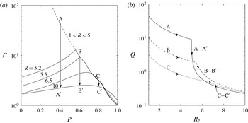
As an example of such a calculation, in figure 9(a) the maximum
 ${\it\Gamma}=QR_{2}$
for stability is shown as a function of
 $P$
for different values of the outer radius of the treatment fluid
 $R_{2}$
. In these calculations, the post-treatment fluid is added to the system when
 $R_{2}=5$
, and the whole process is completed when
 $R_{2}=10$
. During the treatment phase,
 $1<R_{2}<5$
, the maximum flow rate to ensure stability of the system may be found using the single-interface analysis of § 2 (dotted line). However, once the post-treatment fluid starts to be injected, for
 $R_{2}\geqslant 5$
, the stability of the trailing interface should also be taken into account in determining the maximum flow rate for stability of the system. We show how this maximum flow rate changes as a function of
 $R_{2}$
in figure 9(a), illustrating the bounds for the values
 $R_{2}=5.2,5.5,6.5$
and
 $10$
(solid lines) as obtained from the analysis of § 3. For a specific choice of
 $P$
we see that
 ${\it\Gamma}$
needs to be systematically reduced once
 $R_{2}>5$
and both interfaces are migrating through the system, and this has been illustrated schematically with the lines A–
 $\text{A}^{\prime }$
, B–
 $\text{B}^{\prime }$
and C–
 $\text{C}^{\prime }$
.
Time to sweep to
 $R_{2}=10$
scaled with the time taken for a single interface in which post-treatment fluid displaces the original reservoir fluid for a series of increasing
 $S$
as a function of the ratio of the leading viscosity jump to the global viscosity jump. The optimum viscosity choice balances the adverse viscosity ratios at the leading and trailing interfaces.

For clarity, in figure 9(b) we illustrate how
 $Q={\it\Gamma}/R_{2}$
varies as
 $R_{2}$
increases, following each of the lines A–
 $\text{A}^{\prime }$
, B–
 $\text{B}^{\prime }$
and C–
 $\text{C}^{\prime }$
from figure 9(a). It is seen that for larger values of
 $P$
(e.g. curve C–
 $\text{C}^{\prime }$
), the maximum stable flow rate during the treatment phase,
 $R_{2}<5$
, is smaller but as
 $R_{2}$
increases further during the clean-up phase, and the trailing interface becomes rate-limiting, the maximum flow rate may be smaller for smaller values of
 $P$
. The trade-off between these early and late time effects can lead to a choice of
 $P$
that minimises the overall time taken to inject the treatment fluid.
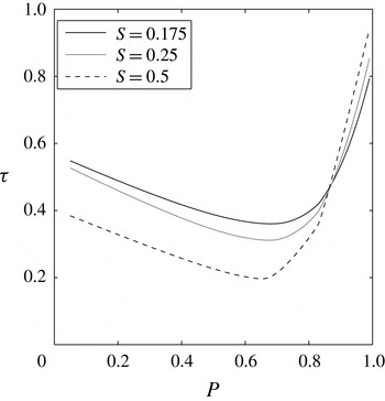
In order to illustrate this trade-off, in figure 10 we show the total injection time required for the leading interface to reach the value
 $R_{2}=10$
as a function of the viscosity of the treatment fluid, as parameterised by
 $P$
. Curves have been shown for different values of the ratio of the volume of treatment fluid to the total volume of fluid injected, as parameterised by
 $S=1-\hat{R}^{2}$
. The overall time taken to sweep is found by integrating
 $Q(R_{2})$
. For each case, there is an overall optimum viscosity for the treatment fluid. Note that in the figure, time is scaled with the time it would take to inject the same total volume of fluid with a single interface between the reservoir fluid and the post-treatment fluid (cf. (2.13)). As
 $S$
becomes larger, the optimal value of
 $P$
decreases; this is because the effect of the instability at the trailing interface becomes smaller since less post-treatment fluid is added, and the interfacial tension on this trailing interface is more effective for smaller radii. Therefore, there is benefit in preferentially increasing the viscosity of the treatment fluid to maximise the average injection rate.
As an illustration of the potential benefits of this analysis in terms of injection time, we note that for example, in the case
 $S=0.25$
, by increasing the viscosity of the treatment fluid to the optimal viscosity, the minimum injection time to maintain overall stability is about 30 % of the injection time when the treatment fluid has the same viscosity as the post-treatment fluid.
5. Conclusions
We have considered the stability of an annulus of fluid spreading from a point source in a Hele-Shaw geometry, in which there is an increase in viscosity across both the leading and trailing interfaces, so that both interfaces are potentially unstable. In a reference calculation of a single interface spreading axisymmetrically from a point source, we show that the stretching of the interface associated with the radial flow permits absolute stability for lower azimuthal modes for sufficiently small viscosity contrasts. We then find a maximum injection rate so that the viscous destabilisation of the interface is suppressed by the combination of the stretching and the interfacial tension for all higher modes.
We build on this analysis for a dual-interface system, in which there may be interactions between instabilities at the leading and trailing interfaces. We find that there is a range of viscosity of the intermediate fluid such that both interfaces are absolutely stable and show how this range depends on the ratio of viscosities of the bounding fluids. We also find the maximum injection rate such that the combination of stretching and interfacial tension is able to suppress the instability of all modes in the system. By following the evolution of this critical flow rate with time during the injection of an annulus of finite volume and a finite volume of the subsequent fluid inside the annulus, we can calculate the minimum total time for injection. We examine how this minimum time varies with the viscosity of the fluid in the annulus, and thereby identify an optimal choice of viscosity that minimises the injection time while maintaining overall stability of the system. We also show how, as the volume of the annulus as a fraction of the total volume of fluid injected increases, the optimal viscosity of the annular fluid increases. Also, the reduction in the time required for the injection of the annular fluid and the following inner fluid relative to the time to inject an equal volume of the inner fluid becomes progressively larger in order to maintain stability.
Although our analysis is strictly valid for Hele-Shaw geometries, the analysis suggests that in field operations in which treatment chemicals are added to a production well for scale management or to suppress sand production, there may be benefit in making the treatment fluid more viscous in order to minimise the time required for the treatment but also to ensure a uniform distribution of the treatment fluid around the well. As a very simplified example, if
 $10~\text{m}^{3}$
of treatment fluid was added to a well followed by
 $10~\text{m}^{3}$
of post-treatment fluid, with an injection rate of
 $0.0001~\text{m}^{3}~\text{s}^{-1}$
, the treatment time would be 30–40 h; by making the treatment fluid more viscous, this process may be accelerated to a time closer to 10–20 h, substantially reducing the non-productive time of the well.
Acknowledgements
The authors wish to thank the three anonymous reviewers who provided very helpful and insightful reviews.