1. Introduction
The mechanics of insect (or bird) flight is a subject of an extensive study (Sane Reference Sane2003; Lehmann Reference Lehmann2004; Wang Reference Wang2005). Hovering flight is a special locomotion in which the body can keep its position largely unchanged at a certain height. There exist two kinds of hovering movements: ‘normal’ hovering, in which the wings of the insect such as hummingbirds move back and forth horizontally and pivot to maintain a favorable angle of attack, and ‘flapping’ hovering, in which the wings flap vertically (Childress, Vandenberghe & Zhang Reference Childress, Vandenberghe and Zhang2006). The ‘flapping’ hovering is normally adopted by birds such as Pied kingfisher, and is thus called ‘avian stroke’ (Azuma Reference Azuma2006). Childress et al. (Reference Childress, Vandenberghe and Zhang2006) experimentally studied the hovering of a passive flapper in a vertically oscillatory flow and suggested that the hovering depends upon a process of the shedding of vortex dipoles closely analogous to that of an active flapper in otherwise still air. Spagnolie & Shelley (Reference Spagnolie and Shelley2009) numerically studied the flow structures and dynamics of an actively shape-changing body subject to an oscillatory flow and demonstrated that the body could hover or ascend by shuttling momentum-carrying vortex dipoles downward into the fluid. Weathers et al. (Reference Weathers, Folie, Liu, Childress and Zhang2010) observed that a rigid pyramid was able to hover stably in an oscillatory air flow at far smaller air amplitudes than would be required by a quasi-steady theory. Liu et al. (Reference Liu, Ristroph, Weathers, Childress and Zhang2012) investigated the stability of flapping flight in a model system that consists of a pyramid-shaped object hovering in a vertically oscillating airflow, and argued that the vortices shed from the body produced the restoring torque for stable hovering. Inspired by the experimental works of Weathers et al. (Reference Weathers, Folie, Liu, Childress and Zhang2010) and Liu et al. (Reference Liu, Ristroph, Weathers, Childress and Zhang2012) on the lift force and the hovering stability of a pyramid-shaped body, we attempt to investigate numerically the dynamics (behaviour of lift force and torque) of an asymmetric body in an oscillating flow in the present study. We think that our numerical results are helpful to better understanding of the experimental results and the hovering mechanism for an asymmetric body. For example, Weathers et al. (Reference Weathers, Folie, Liu, Childress and Zhang2010) observed that the lift force was higher than that predicted from the quasi-steady theory, and simply attributed the reason to the acceleration effect; here we observe that the vortex effect is very important and can be more important than the added mass effect when the Reynolds number is relatively high. Liu et al. (Reference Liu, Ristroph, Weathers, Childress and Zhang2012) conjectured that the sideway jet was responsible for the stable hovering, and our results confirmed this conjecture for the unstable regime, but for the stable regime, we provide a new explanation with the shifts in the positions of the flow stagnation point on the body edge and the projection point of the body mass center on the edge.
Despite being motivated by the hovering problem of Weathers et al. (Reference Weathers, Folie, Liu, Childress and Zhang2010) and Liu et al. (Reference Liu, Ristroph, Weathers, Childress and Zhang2012), our work is related to the fundamental understanding of the steady streaming around an asymmetric body in an oscillatory flow. The time-average of a fluctuating flow often results in a non-zero mean flow, which is referred to as steady streaming (Riley Reference Riley2001). The steady streaming around a circular cylinder for relatively high oscillation frequencies was analyzed by Holtsmark et al. (Reference Holtsmark, Johnsen, Sikkeland and Skavlem1954), Stuart (Reference Stuart1966) and Wang (Reference Wang1968). The structure consists of four small recirculating cells attached on the cylinder surface and four large outer ones further away from the cylinder (Wang Reference Wang1968; Van Dyke Reference Van Dyke1982). The flow structures around a circular cylinder in the vortex shedding regimes at relatively low oscillation frequencies were investigated experimentally (e.g. Williamson Reference Williamson1985; Sarpkaya Reference Sarpkaya1986) and numerically (Iliadis & Anagnostopoulos Reference Iliadis and Anagnostopoulos1998; An, Cheng & Zhao Reference An, Cheng and Zhao2009), and the results showed that different numbers of vortex pairs were shed from the cylinder in the different regimes of the Keulegan–Carpenter (KC) number (i.e. the dimensionless oscillation period). An, Cheng & Zhao (Reference An, Cheng and Zhao2011a ,Reference An, Cheng and Zhao b ) investigated numerically the Honji instability in the three-dimensional flow, and the steady streaming around a circular cylinder near a plane boundary, respectively. Lu, Dalton & Zhang (Reference Lu, Dalton and Zhang1997) applied the large eddy simulation method to the turbulent oscillating flow past a circular cylinder, and the force coefficients calculated were in good agreement with the experiments of Sarpkaya (Reference Sarpkaya1986). Williamson (Reference Williamson1985) investigated experimentally the hydrodynamic interactions between two cylinders in oscillating flows and observed that the vortex-shedding patterns identified for a single cylinder could synchronize either in phase or in anti-phase. Coenen (Reference Coenen2013) analysed the oscillatory flow around a pair of circular cylinders of unequal diameter and observed the jet eruptions from the cylinder surfaces. The oscillatory flows past four circular cylinders were simulated by Anagnostopoulos & Dikarou (Reference Anagnostopoulos and Dikarou2011) and Chern, Shiu & Horng (Reference Chern, Shiu and Horng2013). The steady streaming structures around a square cylinder (Bearman et al. Reference Bearman, Graham, Obasaju and Drossopulos1984; Zheng & Dalton Reference Zheng and Dalton1999), two square cylinders (Chern et al. Reference Chern, Kanna, Lu, Cheng and Chang2010), a sphere (Riley Reference Riley1966; Zhao, Sadhal & Trinh Reference Zhao, Sadhal and Trinh1999) and a spheroid (Rednikov & Sadhal Reference Rednikov and Sadhal2004) have also been investigated. The formation of chains of spherical particles, aligned perpendicular to the direction of oscillation, was observed in the oscillating flow, and the reason was attributed to the steady streaming flow induced by the vibration (Wunenburger, Carrier & Garrabos Reference Wunenburger, Carrier and Garrabos2002; Klotsa et al. Reference Klotsa, Swift, Bowley and King2009; Pacheco-Martinez et al. Reference Pacheco-Martinez, Liao, Hill, Swift and Bowley2013). Wright, Swift & King (Reference Wright, Swift and King2008) investigated the motion of a dimer consisting of a pair of spheres of unequal size and observed that the dimer migrated in the direction perpendicular to the oscillation direction, with the small sphere as a leading one. In the present study, we are mainly concerned with the force on an open triangle in the oscillation direction, the torque in both stable and unstable flow regimes and the steady streaming structures of an asymmetric body, which to our knowledge have not been investigated previously in numerical aspect.
The rest of the paper is organized as follows. We first introduce our numerical method, the numerical model for the problem of interest and the validation of the computational accuracy in § 2. In § 3, the average force and torque coefficients for a fixed open triangle in an oscillatory flow are analysed, and then the free motions of a released open triangle are simulated. Concluding remarks are given in the final section.
2. Numerical model
2.1. Fictitious domain (FD) method
2.1.1. FD formulation
The direct-forcing fictitious domain (DF/FD) method used in the present study was proposed by Yu & Shao (Reference Yu and Shao2007), who developed the method from new implementations of the FD formulation of Glowinski et al. (Reference Glowinski, Pan, Hesla and Joseph1999) for the particulate flows. The key idea of the method is that the interior of the solid body is assumed to be filled with the fluid and the inner fictitious fluid is constrained to move at the same velocity with the body by a pseudo body force (i.e. Lagrange multiplier). We only briefly describe the algorithm of the DF/FD method in the following and the reader is referred to Yu & Shao (Reference Yu and Shao2007) for the details of the method.
For simplicity of description, we consider only one particle (or body) in two dimensions in the following. Suppose that the particle density, area, moment of inertia tensor, translational velocity and angular velocity are denoted by
 ${\it\rho}_{p}$
,
 $S_{p}$
,
 $J$
,
 $\boldsymbol{U}$
and
 ${\it\omega}_{p}$
, respectively. The fluid viscosity and density are
 ${\it\mu}$
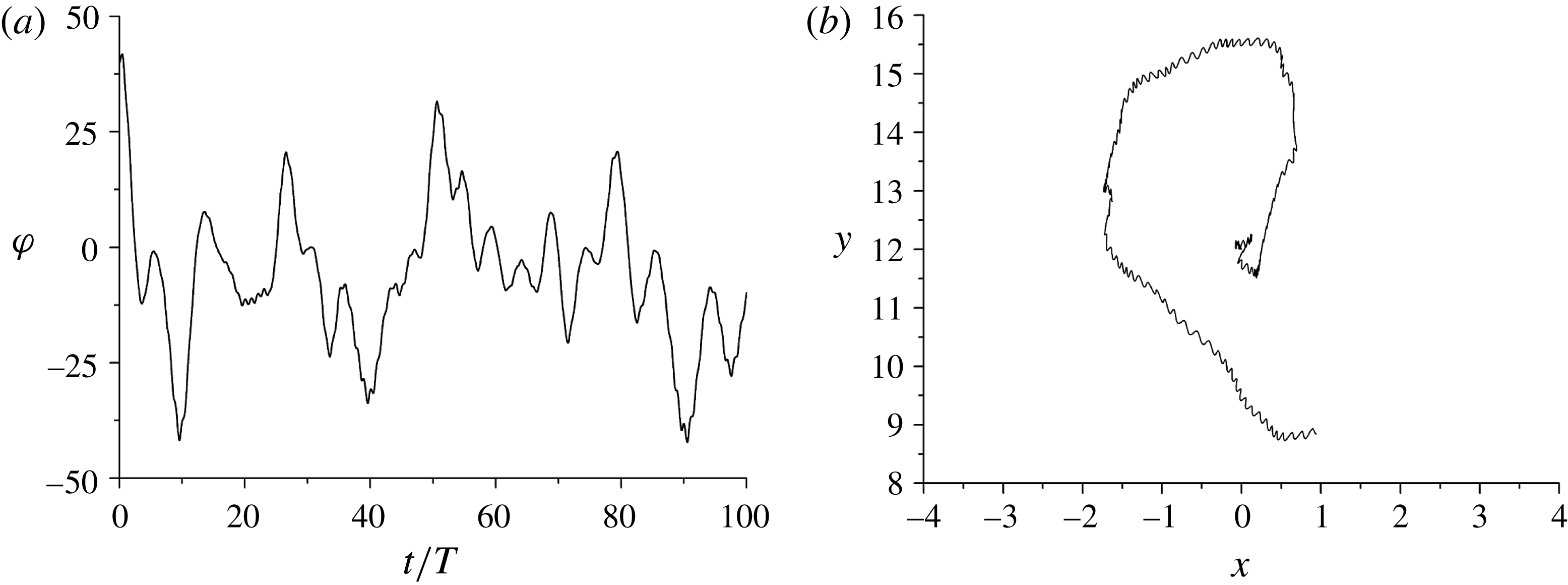
and
 ${\it\rho}_{f}$
, respectively. Let
 $P(t)$
represent the solid domain and
 ${\it\Omega}$
the entire domain including interior and exterior of the solid body. By introducing the following scales for the non-dimensionalization:
 $L_{c}$
for length,
 $U_{c}$
for velocity,
 $L_{c}/U_{c}$
for time,
 ${\it\rho}_{f}U_{c}^{2}$
for the pressure and
 ${\it\rho}_{f}U_{c}^{2}/L_{c}$
for the pseudo body-force, the dimensionless FD formulation for the incompressible fluid can be written as follows:
 $$\begin{eqnarray}\displaystyle & \displaystyle \frac{\partial \boldsymbol{u}}{\partial t}+\boldsymbol{u}\boldsymbol{\cdot }\boldsymbol{{\rm\nabla}}\boldsymbol{u}=\frac{{\rm\nabla}^{2}\boldsymbol{u}}{Re}-\boldsymbol{{\rm\nabla}}p+{\it\lambda}\quad \text{in }{\it\Omega}, & \displaystyle\end{eqnarray}$$
 $$\begin{eqnarray}\displaystyle & \displaystyle \boldsymbol{u}=\boldsymbol{U}+{\it\omega}_{p}\times \boldsymbol{r}\quad \text{in }P(t), & \displaystyle\end{eqnarray}$$
 $$\begin{eqnarray}\displaystyle & \displaystyle \boldsymbol{{\rm\nabla}}\boldsymbol{\cdot }\boldsymbol{u}=0\quad \text{in }{\it\Omega}, & \displaystyle\end{eqnarray}$$
 $$\begin{eqnarray}\displaystyle & \displaystyle ({\it\rho}_{r}-1)S_{p}^{\ast }\left(\frac{\text{d}\boldsymbol{U}}{\text{d}t}-Fr\frac{\boldsymbol{g}}{g}\right)=-\!\int _{P}{\it\lambda}\,\text{d}\boldsymbol{x}, & \displaystyle\end{eqnarray}$$
 $$\begin{eqnarray}\displaystyle & \displaystyle ({\it\rho}_{r}-1)J^{\ast }\frac{\text{d}{\it\omega}_{p}}{\text{d}t}=-\!\int _{P}\boldsymbol{r}\times {\it\lambda}\,\text{d}\boldsymbol{x}. & \displaystyle\end{eqnarray}$$
 $\boldsymbol{u}$
represents the fluid velocity,
 $p$
the fluid pressure,
 ${\it\lambda}$
the pseudo body-force that is defined in the solid domain
 $P(t)$
,
 $\boldsymbol{r}$
the position vector with respect to the mass centre of the particle,
 ${\it\rho}_{r}$
the particle–fluid density ratio defined by
 ${\it\rho}_{r}={\it\rho}_{p}/{\it\rho}_{f}$
,
 $Re$
the Reynolds number defined by
 $Re={\it\rho}_{f}U_{c}L_{c}/{\it\mu}$
,
 $Fr$
the Froude number defined here by
 $Fr=gL_{c}/U_{c}^{2}$
,
 $S_{p}^{\ast }$
the dimensionless body area defined by
 $S_{p}^{\ast }=S_{p}/L_{c}^{2}$
and
 $J^{\ast }$
the dimensionless moment of inertia defined by
 $J^{\ast }=J/{\it\rho}_{p}L_{c}^{4}$
. Note that for the two-dimensional case, in (2.5)
 $\boldsymbol{r}\times {\it\lambda}$
actually represents its non-zero component
 $x{\it\lambda}_{y}-y{\it\lambda}_{x}$
, and we retain the vector form for convenience.
The force and torque on the body exerted by the fluid in the dimensional form can be computed with the pseudo body-force as follows:
 $$\begin{eqnarray}\displaystyle & \displaystyle \boldsymbol{F}={\it\rho}_{f}S_{p}\frac{\text{d}\boldsymbol{U}}{\text{d}t}-\!\int _{P}{\it\lambda}\,\text{d}\boldsymbol{x}, & \displaystyle\end{eqnarray}$$
 $$\begin{eqnarray}\displaystyle & \displaystyle M={\it\rho}_{f}\frac{J}{{\it\rho}_{p}}\frac{\text{d}{\it\omega}_{p}}{\text{d}t}-\!\int _{P}\boldsymbol{r}\times {\it\lambda}\,\text{d}\boldsymbol{x}. & \displaystyle\end{eqnarray}$$
2.1.2. Numerical schemes
A fractional-step time scheme is used to decouple the system (2.1)–(2.5) into the following two sub-problems.
Fluid sub-problem for
 $\boldsymbol{u}^{\ast }$
and
 $p$
:
 $$\begin{eqnarray}\displaystyle & \displaystyle \frac{\boldsymbol{u}^{\ast }-\boldsymbol{u}^{n}}{{\rm\Delta}t}-\frac{1}{2}\frac{{\rm\nabla}^{2}\boldsymbol{u}^{\ast }}{Re}=-\boldsymbol{{\rm\nabla}}p+\frac{1}{2}[3(\boldsymbol{u}\boldsymbol{\cdot }\boldsymbol{{\rm\nabla}}\boldsymbol{u})^{n}-(\boldsymbol{u}\boldsymbol{\cdot }\boldsymbol{{\rm\nabla}}\boldsymbol{u})^{n-1}]+\frac{1}{2}\frac{{\rm\nabla}^{2}\boldsymbol{u}^{n}}{Re}+{\it\lambda}^{n}, & \displaystyle\end{eqnarray}$$
 $$\begin{eqnarray}\displaystyle & \displaystyle \boldsymbol{{\rm\nabla}}\boldsymbol{\cdot }\boldsymbol{u}^{\ast }=0. & \displaystyle\end{eqnarray}$$
Particle sub-problem for
 $\boldsymbol{U}^{n+1}$
,
 ${\it\omega}_{p}^{n+1}$
,
 ${\it\lambda}^{n+1}$
,
 $\boldsymbol{u}^{n+1}$
:
 $$\begin{eqnarray}\displaystyle & \displaystyle {\it\rho}_{r}S_{p}^{\ast }\frac{\boldsymbol{U}^{n+1}}{{\rm\Delta}t}=({\it\rho}_{r}-1)S_{p}^{\ast }\left(\frac{\boldsymbol{U}^{n}}{{\rm\Delta}t}-Fr\frac{\boldsymbol{g}}{g}\right)+\int _{P}\left(\frac{\boldsymbol{u}^{\ast }}{{\rm\Delta}t}-{\it\lambda}^{n}\right)\,\text{d}\boldsymbol{x}, & \displaystyle\end{eqnarray}$$
 $$\begin{eqnarray}\displaystyle & \displaystyle {\it\rho}_{r}\frac{J^{\ast }{\it\omega}_{p}^{n+1}}{{\rm\Delta}t}=({\it\rho}_{r}-1)\frac{J^{\ast }{\it\omega}_{p}^{n}}{{\rm\Delta}t}+\int _{P}\boldsymbol{r}\times \left(\frac{\boldsymbol{u}^{\ast }}{{\rm\Delta}t}-{\it\lambda}^{n}\right)\,\text{d}\boldsymbol{x}. & \displaystyle\end{eqnarray}$$
 $\boldsymbol{U}^{n+1}$
and
 ${\it\omega}_{p}^{n+1}$
are obtained without iteration.
Then,
 ${\it\lambda}^{n+1}$
defined at the Lagrangian nodes are determined from
 $$\begin{eqnarray}{\it\lambda}^{n+1}=\frac{\boldsymbol{U}^{n+1}+{\it\omega}_{p}^{n+1}\times \boldsymbol{r}-\boldsymbol{u}^{\ast }}{{\rm\Delta}t}+{\it\lambda}^{n}\end{eqnarray}$$
and finally, the fluid velocities
 $\boldsymbol{u}^{n+1}$
at the Eulerian nodes are obtained from
 $$\begin{eqnarray}\boldsymbol{u}^{n+1}=\boldsymbol{u}^{\ast }+{\rm\Delta}t({\it\lambda}^{n+1}-{\it\lambda}^{n}).\end{eqnarray}$$
In the above manipulations, the bi-linear function is used to interpolate the fluid velocity from the Eulerian nodes to the Lagrangian nodes, and to distribute the pseudo body-force from the Lagrangian nodes to the Eulerian nodes.
Note that we are mainly concerned with the force and torque on a fixed body in an oscillatory flow in the present study, for which case one just needs to set the body’s velocities to be zero in (2.6), (2.7) and (2.12), namely,
 $\boldsymbol{U}={\it\omega}_{p}=0$
, and the solutions of the body’s velocities (2.10), (2.11) are not necessary.
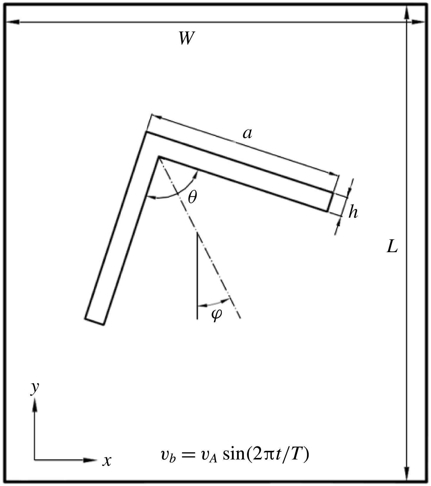
Schematic diagram of the problem studied. The oscillatory flow is in the
 $y$
-axis direction.

2.2. Numerical model
Figure 1 delineates the schematic diagram of the problem involving an open isosceles triangle (or a
 $\wedge$
-shaped body) in an oscillatory flow. The edge length of the open triangle is denoted by
 $a$
, the edge thickness
 $h$
, the vertex angle
 ${\it\theta}$
, and the tilt angle between the triangle’s axis of symmetry and the
 $y$
-axis
 ${\it\varphi}$
. We use
 ${\it\varphi}_{0}$
to denote the tilt angle
 ${\it\varphi}$
at initial time or for the case of fixed triangle. The width of the computational domain is
 $W$
and the height is
 $L$
. To simulate the oscillatory flow, the velocity
 $v_{b}$
is imposed at four boundaries of the computational domain in the
 $y$
-axis direction:
 $$\begin{eqnarray}v_{b}=v_{A}\sin (2{\rm\pi}t/T),\end{eqnarray}$$
where
 $v_{A}$
is the amplitude of the velocity and
 $T$
is the period. Such Dirichlet boundary condition is equivalent to the oscillation of a body in an enclosed box, and the far-field boundaries are required to be located far away from the body to make their confinement effect negligible.
We take the edge length
 $a$
as the characteristic length and
 $v_{A}$
as the characteristic velocity for the non-dimensionlization. The dimensionless physical control parameters are the Reynolds number, defined as
 $Re={\it\rho}_{f}v_{A}a/{\it\mu}$
and the dimensionless period, defined as
 $T^{\ast }=Tv_{A}/a$
, which is also called Keulegan–Carpenter (KC) number (Iliadis & Anagnostopoulos Reference Iliadis and Anagnostopoulos1998; An et al.
Reference An, Cheng and Zhao2011a
,Reference An, Cheng and Zhao
b
). The dimensionless period
 $T^{\ast }$
also reflects the longest distance that the fluid moves in one oscillation period (i.e. peak-to-peak displacement)
 $A$
with respect to the body size
 $a$
, since
 $$\begin{eqnarray}\frac{A}{a}=\frac{1}{a}\int _{0}^{T/2}v_{A}\sin \left(\frac{2{\rm\pi}t}{T}\right)\,\text{d}t=\frac{Tv_{A}}{a{\rm\pi}}=\frac{T^{\ast }}{{\rm\pi}}.\end{eqnarray}$$
We examine the effects of
 $T^{\ast }$
in the range of 2–10, as typically in the previous experimental studies (Weathers et al.
Reference Weathers, Folie, Liu, Childress and Zhang2010; Liu et al.
Reference Liu, Ristroph, Weathers, Childress and Zhang2012). Throughout the present study, the edge thickness is fixed to be
 $h=0.06a$
. It is difficult to ensure the computational accuracy for a very small
 $h/a$
. The size of the computational domain is
 $12a\times 24a$
. The increase in the size of the computational domain is found not to bring about significant difference in the results. The mesh number of
 $1024\times 2048$
(homogeneous mesh) and the time-step of
 $0.002a/v_{A}$
are employed.
The vertical force and torque coefficients are defined as
 $$\begin{eqnarray}\displaystyle & \displaystyle C_{y}=\frac{F_{y}}{0.5{\it\rho}_{f}v_{A}^{2}a}, & \displaystyle\end{eqnarray}$$
 $$\begin{eqnarray}\displaystyle & \displaystyle C_{m}=\frac{M}{0.5{\it\rho}_{f}v_{A}^{2}a}. & \displaystyle\end{eqnarray}$$
 $$\begin{eqnarray}\displaystyle & \displaystyle \overline{C_{y}}(t_{0})=\frac{1}{T}\int _{t_{0}-T}^{t_{0}}C_{y}(t)\,\text{d}t, & \displaystyle\end{eqnarray}$$
 $$\begin{eqnarray}\displaystyle & \displaystyle \overline{C_{m}}(t_{0})=\frac{1}{T}\int _{t_{0}-T}^{t_{0}}C_{m}(t)\,\text{d}t, & \displaystyle\end{eqnarray}$$
 $t_{0}=NT$
,
 $N$
being a positive integer.
2.3. Validation
Two test problems are chosen to validate the accuracy of our computations: the oscillatory flows over a circular cylinder and an open triangle, respectively.
2.3.1. Circular cylinder
The numerical model is the same as the open triangle problem plotted in figure 1, except that the triangle is replaced with a circular cylinder with the diameter
 $D$
being unity. For the test case, the Reynolds number is 200, and the size of the computational domain is
 $20D\times 20D$
. For our DF/FD computations, the mesh size is
 $D/51.2$
and the time-step is
 $0.002D/v_{A}$
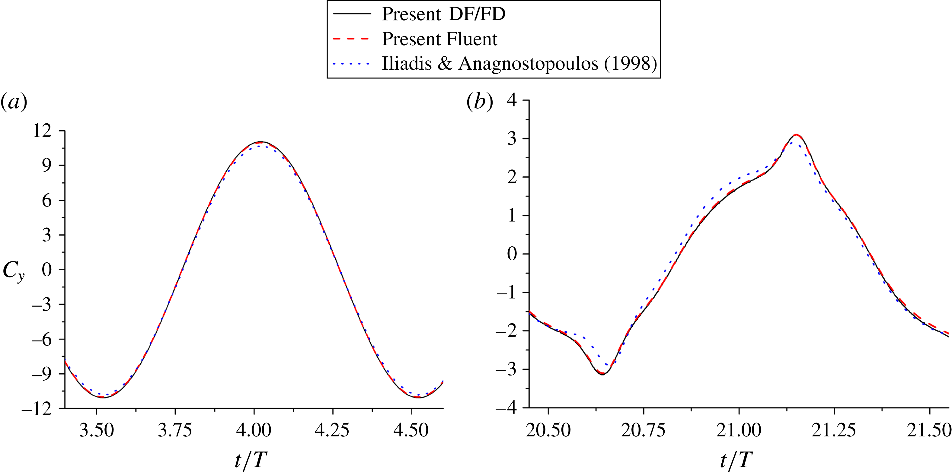
, which were tested to produce mesh-size and time-step independent results. Our results on the instantaneous vertical force coefficients for
 $T^{\ast }=2$
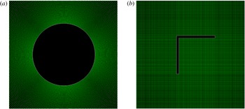
and 10 are compared to those of Iliadis & Anagnostopoulos (Reference Iliadis and Anagnostopoulos1998) in figure 2. An apparent discrepancy between two results can be seen, therefore, we conduct computations with Fluent commercial software using a fine structured mesh, as shown in figure 3(a). Figure 2 shows that our results are in good agreement with the Fluent computations.
Evolutions of the instantaneous force coefficients in the
 $y$
-direction for a circular cylinder in an oscillatory flow at (a)
 $T^{\ast }=2$
and (b)
 $T^{\ast }=10$
, as compared to the results of Fluent computations and Iliadis & Anagnostopoulos (Reference Iliadis and Anagnostopoulos1998).
 $Re=200$
.

Mesh near the body used in Fluent computations for (a) circular cylinder and (b) open triangle.

2.3.2. Open triangle
In this validation the body is an open triangle with the vertex angle
 ${\it\theta}=90^{\circ }$
, the edge length
 $a=1$
, the edge thickness
 $h=0.06$
and the initial tilt angle
 ${\it\varphi}_{0}=45^{\circ }$
, for which a structured mesh can be generated for the Fluent computations, as shown in figure 3(b). The Reynolds number
 $Re$
is 50, the dimensionless period is 2, and the size of the computational domain is
 $12a\times 24a$
. The mesh number and time-step for our DF/FD computations are
 $1024\times 2048$
and
 $0.002a/v_{A}$
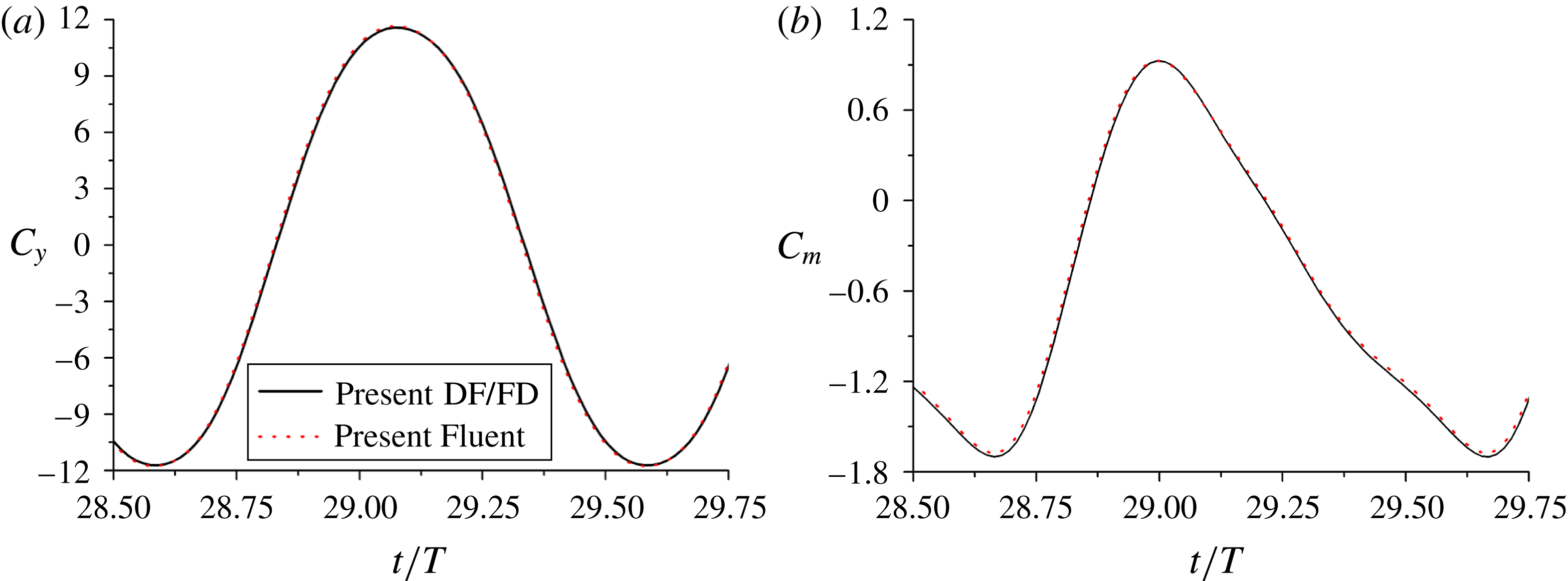
, respectively. The mesh-size and time-step convergences have been checked for both DF/FD and Fluent results. The time-developments of the vertical force and torque coefficients are shown in figure 4(a,b), respectively. Our DF/FD results agree well with the Fluent results. We choose DF/FD method rather than the Fluent computation for the present study because it is more efficient (mainly due to the faster solver for the Poisson equation in the DF/FD method while the iteration at every time step required for Fluent), more convenient (it is not easy to generate high quality structured mesh for the Fluent computations for other configurations of the body rather than the case in figure 3
b), and more flexible (the motion of the body can be easily coped with our DF/FD method, but not Fluent).
Time-developments of (a) vertical force coefficient and (b) torque coefficient obtained with our DF/FD and Fluent computations respectively for an open triangle in an oscillatory flow.
 $Re=50$
,
 $T^{\ast }=2$
.

3. Results and discussion
Our primary aim is to better understand the underlying mechanisms on the stable hovering of an asymmetrical body in an oscillatory flow, but the direct analysis of the dynamics of a freely moving body is difficult, thus we mainly examine the behaviour of the force and torque on a fixed body.
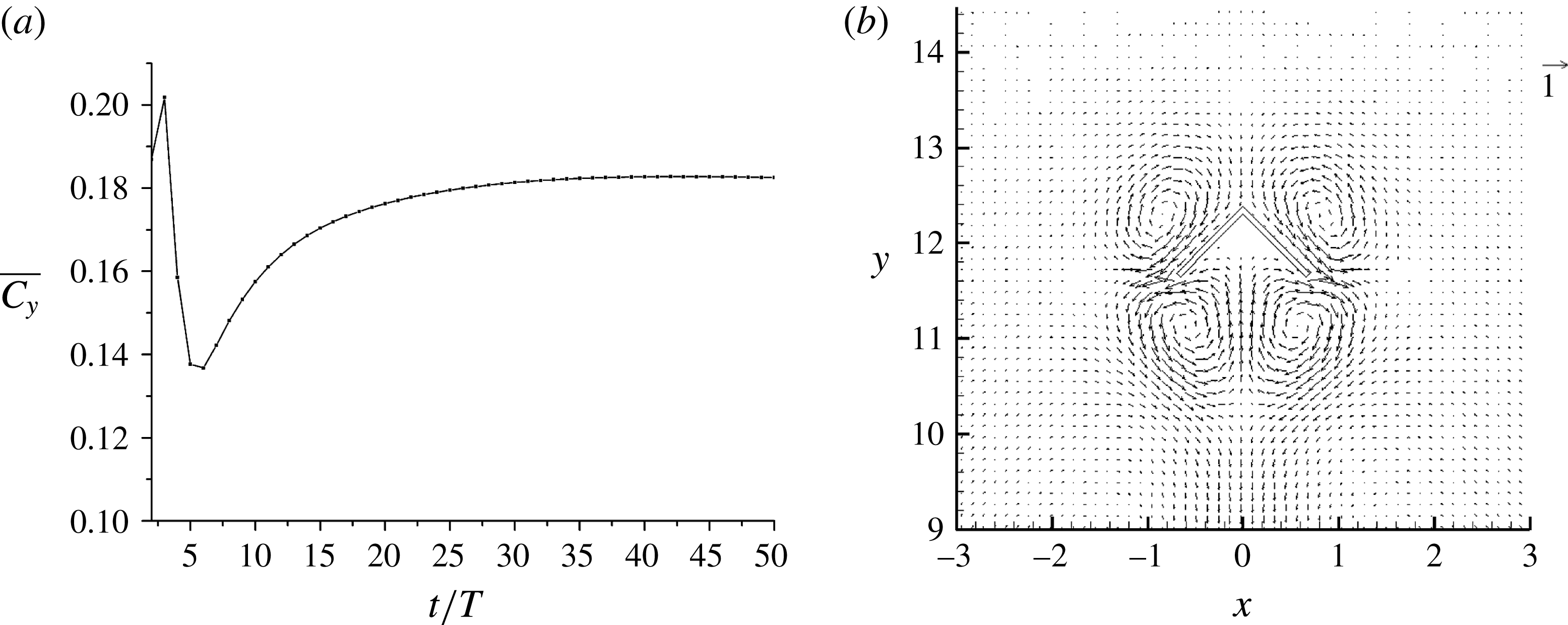
(a) Evolution of the period-averaged vertical force coefficient for an upright open triangle at
 $Re=50$
,
 ${\it\theta}=90^{\circ }$
,
 ${\it\varphi}_{0}=0$
, and
 $T^{\ast }=4$
, and (b) the corresponding average velocity vectors at stable state.

3.1. Vertical force coefficient
The vertical force on the body is analysed in this subsection. The vertical force can be regarded as the lift force for the hovering body, but it is essentially a drag force since the force points to the flow direction. For simplicity, the vertical force is analysed at the most typical configuration of the hovering body: the upright orientation. As one will see, the behaviour of the force and torque on the body depends heavily on whether the flow is stable or not. Therefore, we discuss our results in the stable and unstable flow regimes, respectively.
3.1.1. Stable flow regime
For relatively low Reynolds numbers and small oscillation periods, the flow can reach a stable state in which the flow fields and the force on the body change in the exactly same way for each period, and thus the period-averaged force can achieve a constant value, as shown in figure 5(a). It has been well recognized that an oscillatory flow can result in a non-zero mean flow, called steady streaming (Riley Reference Riley2001). The period-averaged velocity fields at stable state for
 $Re=50$
,
 ${\it\theta}=90^{\circ }$
and
 $T^{\ast }=4$
are plotted in figure 5(b), which shows that the steady streaming structure for the
 $\wedge$
-shaped body is mainly composed of 4 circulations (or 4 vortices) near the body. The steady streaming structure for a cylinder (Wang Reference Wang1968; Van Dyke Reference Van Dyke1982) or a sphere (Rednikov & Sadhal Reference Rednikov and Sadhal2004; Pacheco-Martinez et al.
Reference Pacheco-Martinez, Liao, Hill, Swift and Bowley2013) consists of four small circulating cells attached on the body surface and four large outer ones further away from the body, when
 $T^{\ast }$
is small. For our case with
 $T^{\ast }=4$
, the size of the inner circulations is comparable to the body size, since the fluid can travel a distance more than
 $a$
in one oscillation period for
 $T^{\ast }=4$
, according to (2.15). The outer circulations are weak, particularly the upper pair, which are invisible in figure 5(b). The lower outer pair is evidenced from the outer downward jet, which also implies an upward force on the body.
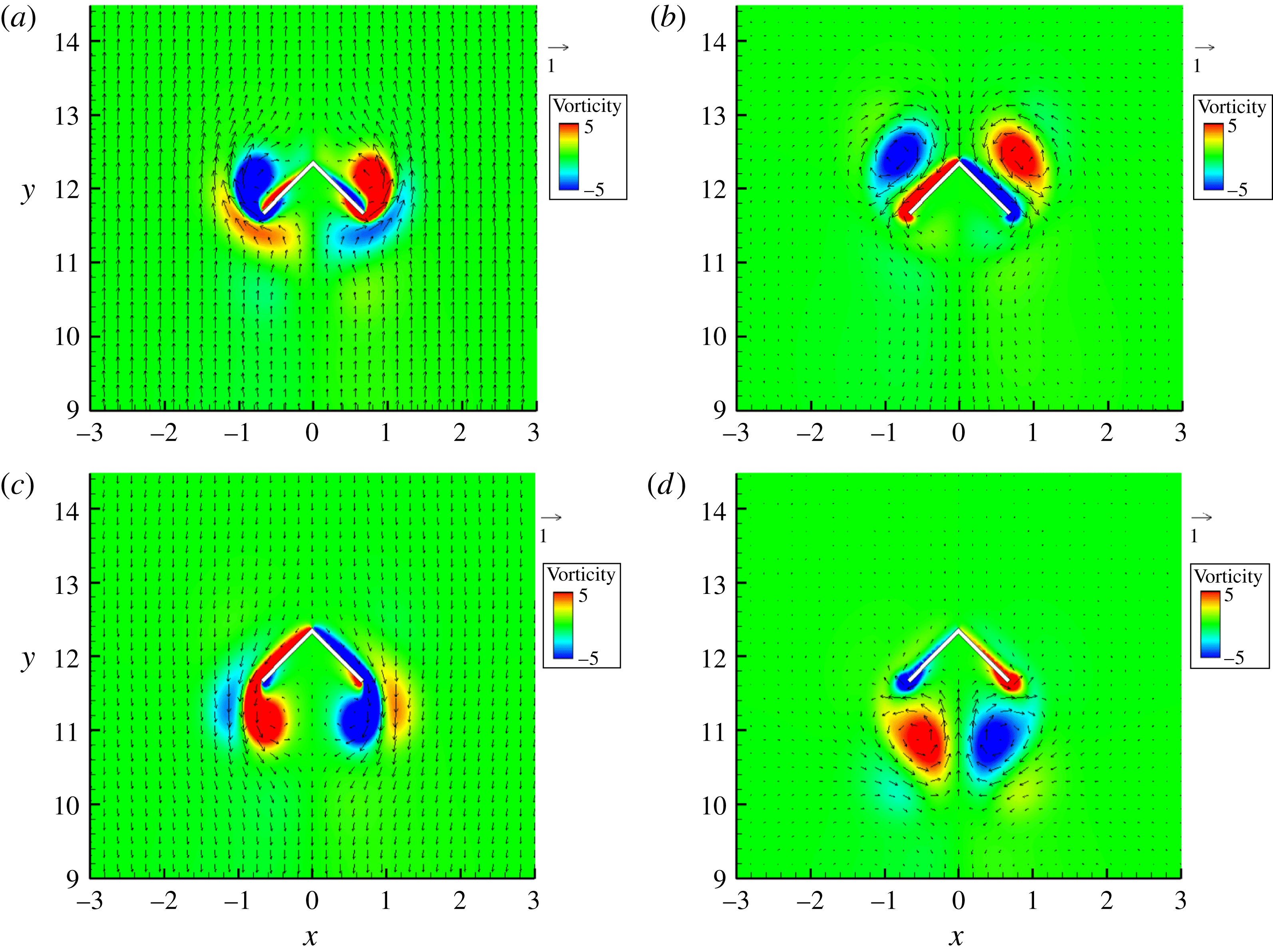
Velocity vectors and vorticity contours at four time moments in one period (a)
 $t^{\prime }=0.25T$
, (b)
 $t^{\prime }=0.5T$
, (c)
 $t^{\prime }=0.75T$
and (d)
 $t^{\prime }=T$
for
 $Re=50$
,
 ${\it\theta}=90^{\circ }$
and
 $T^{\ast }=4$
.

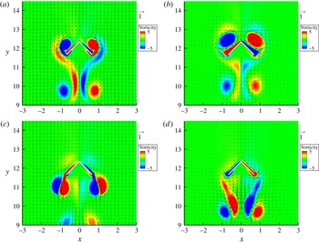
The velocity vectors and vorticity contours at four time moments in one period
 $t^{\prime }=0.25T$
,
 $0.5T$
,
 $0.75T$
and
 $T$
are plotted in figure 6. Here,
 $t^{\prime }$
denotes the time within one period. Recalling that
 $v_{b}=v_{A}\sin (2{\rm\pi}t/T)$
, the fluid moves upward for
 $t^{\prime }=0{-}0.5T$
with the maximum velocity at
 $t^{\prime }=0.25T$
, and downward for
 $t^{\prime }=0.5T{-}T$
with the maximum velocity at
 $t^{\prime }=0.75T$
. From figure 6, a strong vortex has formed at each side of the body by
 $t^{\prime }=0.25T$
when the undisturbed velocity reaches maximum and has shed from the body by
 $t^{\prime }=0.5T$
when the velocity is deceased to zero. This shed vortex then moves downward in the following downward flow phase, but its intensity becomes much weaker than the vortex newly forming during downward flow for
 $Re=50$
(figure 6
c). The formation and evolution of the flow structures are similar for the upward and downward flow stages, but the vortex structures at two phases are not up–down symmetrical due to geometrical asymmetry of the body. For
 $Re=50$
, the newly-shed vortices dominate the flow near the body and are apparently responsible for the steady steaming structures shown in figure 5(b). As the Reynolds number is increased to be 125, the vortex shed during upward flow becomes so strong that at
 $t^{\prime }=0.75T$
its intensity is comparable to the vortex forming during downward flow, and it looks as if a pair of vortices are emitted from each edge of the body, as shown in figure 11 and observed in experiments (their figure 2) of Liu et al. (Reference Liu, Ristroph, Weathers, Childress and Zhang2012). For the stable flow regime, the flow structures retain the left–right symmetry, whereas for the unstable regime, the left–right symmetry is lost and the flow becomes chaotic due to complex interactions between vortices, which will be discussed later.
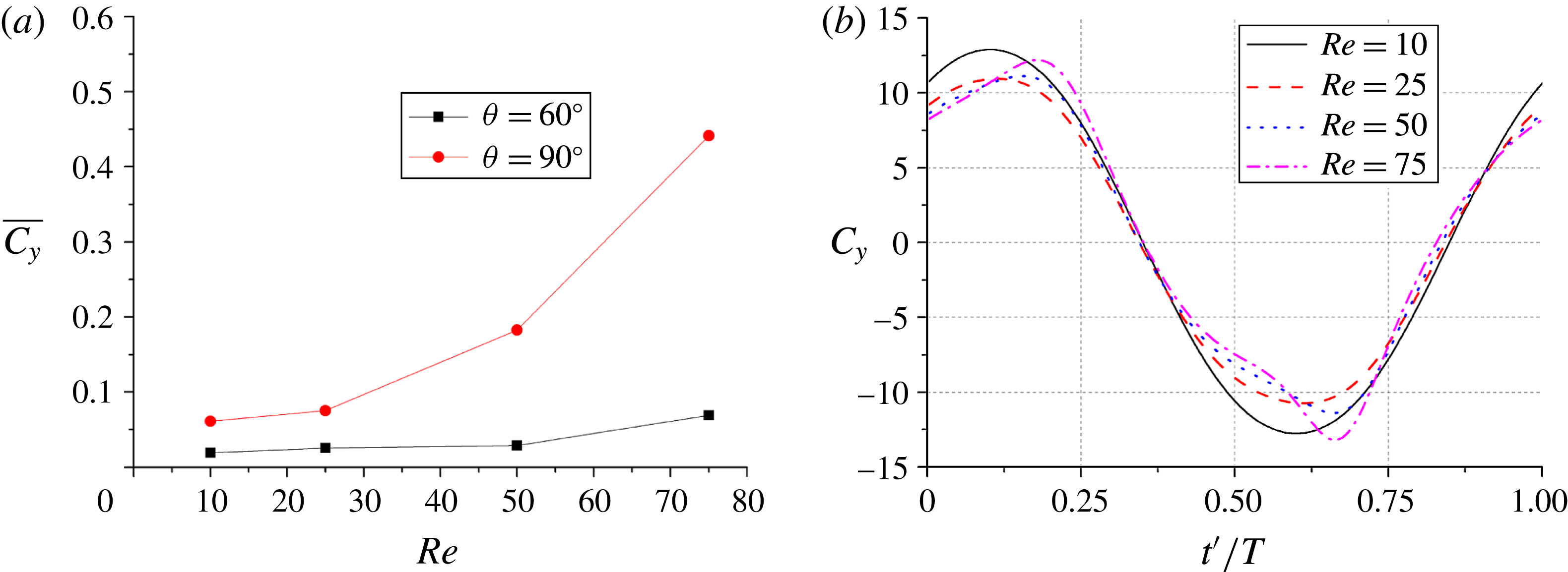
(a) Average vertical force coefficients as a function of Reynolds number for
 ${\it\theta}=60^{\circ }$
and 90°, and (b) instantaneous force coefficients in one period for
 ${\it\theta}=90^{\circ }$
and different Reynolds numbers.
 $T^{\ast }=4$
and
 ${\it\varphi}_{0}=0$
.

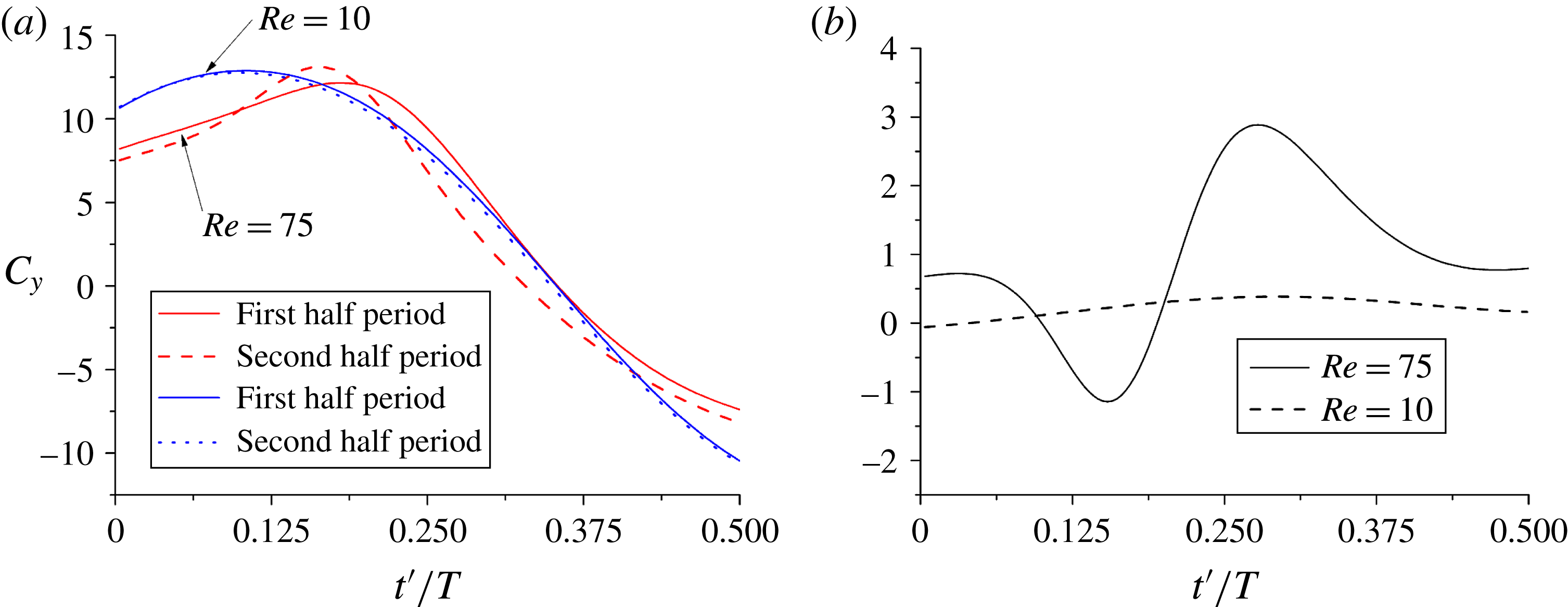
Comparison of (a) the instantaneous force coefficients in the upward flow phase (i.e. first half period) and downward flow phase (i.e. second half period) and (b) their differences for
 $Re=10$
and 75. The time for the force coefficients in the second half period is a shifted half period with the sign of the coefficients reversed for comparison (i.e. the direction of the force is defined as the same of the velocity).
 ${\it\theta}=90^{\circ }$
,
 ${\it\varphi}_{0}=0$
and
 $T^{\ast }=4$
.

We now examine the effects of the Reynolds number on the vertical force. Figure 7(a) shows the average vertical force coefficients for
 $Re=10{-}75$
,
 $T^{\ast }=4$
, and
 ${\it\theta}=60^{\circ }$
and 90°. We see that the average vertical force increases with increasing Reynolds number. To elucidate the mechanism, the instantaneous force coefficients in one period for
 ${\it\theta}=90^{\circ }$
and different Reynolds numbers are plotted in figure 7(b). Theoretically speaking, the force on the body in the oscillatory flow mainly comprises two types of force: quasi-steady drag force and added mass force from the fluid acceleration. The quasi-steady drag should change in phase with the velocity, and the added mass force should change in phase with the fluid acceleration. The maximum upward acceleration and velocity take place at
 $t^{\prime }=0$
and
 $t^{\prime }=0.25T$
, respectively. Thus, the positive force peak occurs between
 $t^{\prime }=0$
and
 $t^{\prime }=0.25T$
in figure 7(b). As the Reynolds number increases, the peak moves toward
 $t^{\prime }=0.25T$
, indicating the quasi-steady drag force might become relatively more important for higher Reynolds numbers. The quasi-steady drag force from the unidirectional upward-flow is larger than the downward-flow (Weathers et al.
Reference Weathers, Folie, Liu, Childress and Zhang2010), and this fact can account for the reason why the period-averaged force is positive. However, the quasi-steady drag force cannot explain why the average force increases with increasing Reynolds number and why the force peak increases as the Reynolds number increases from 25 to 75 in figure 7(b). Considering that the average force is caused by the difference between the instantaneous forces during upward and downward flow stages, we directly compare the instantaneous force coefficients for two flow stages for
 $Re=10$
and 75 by shifting the data in the second half period (downward-flow) to the first half period and changing their signs in figure 8(a). For
 $Re=10$
, the curve shapes for two phases are similar, and the maximum difference in the forces occurs at around
 $t^{\prime }=0.25T$
(at exactly
 $t^{\prime }=0.29T$
from our data and also from figure 8
b), which can be roughly explained with the up–down asymmetry of the quasi-steady drag force. In contrast, for
 $Re=75$
, there is a pronounced difference in the curve shapes for two flow stages, and the average force is mainly a result of the difference during the velocity-decreasing phase (i.e.
 $t^{\prime }=0.25T{-}0.5T$
), as can be seen from figure 8(a,b). The velocity-decreasing phase is characterized by the presence of the strong vortices near the body, as discussed earlier and shown in figure 6. The vortex-induced flow causes additional force on the body. The difference in the vortices for two flow stages can be reflected in the steady streaming structure in figure 5(b), and we think that the flow induced by the bottom vortex pair can give rise to larger force on the body than by the upper pair, due to the more streamlined shape of the body for downward flow, which is the same reason for the difference in the quasi-steady drag force. The fact that the vortex intensity increases with increasing Reynolds number explains why the vertical force increases with Reynolds number. Weathers et al. (Reference Weathers, Folie, Liu, Childress and Zhang2010) observed that the average vertical force on a hollow pyramid in an oscillatory flow was underestimated from the quasi-steady force theory and conjectured that the acceleration might account for the disparity. From our numeric results above, the enhancement in the average force on the body is mainly the result of the effects of the vortices.
Figure 7(a) shows that the average vertical force for
 ${\it\theta}=90^{\circ }$
is significantly larger than that for
 ${\it\theta}=60^{\circ }$
. Because the length of the body edge
 $a$
is fixed, the body with a larger vertex angle has a larger horizontal span, which not only enhances the upwinding area of the body but also provides a bigger space for the vortices to develop. Therefore, the vertical force (thereby the coefficient normalized with
 $a$
) from both viscous drag and vortices can increase with increasing vertex angle for a certain range of vertex angle. Considering that both
 ${\it\theta}=0^{\circ }$
and 180° correspond to the configuration of up–down symmetry,
 ${\it\theta}=90^{\circ }$
might be regarded as the configuration of least up–down symmetry. The average vertical force is expected to decrease as the vertex angle approaches 180° as a result of the decrease in the up–down asymmetry.
(a) Average vertical force coefficients as a function of dimensionless period for
 ${\it\theta}=60^{\circ }$
and 90°and (b) instantaneous force coefficients in one period for different periods and
 ${\it\theta}=90^{\circ }$
.
 $Re=50$
and
 ${\it\varphi}_{0}=0$
.

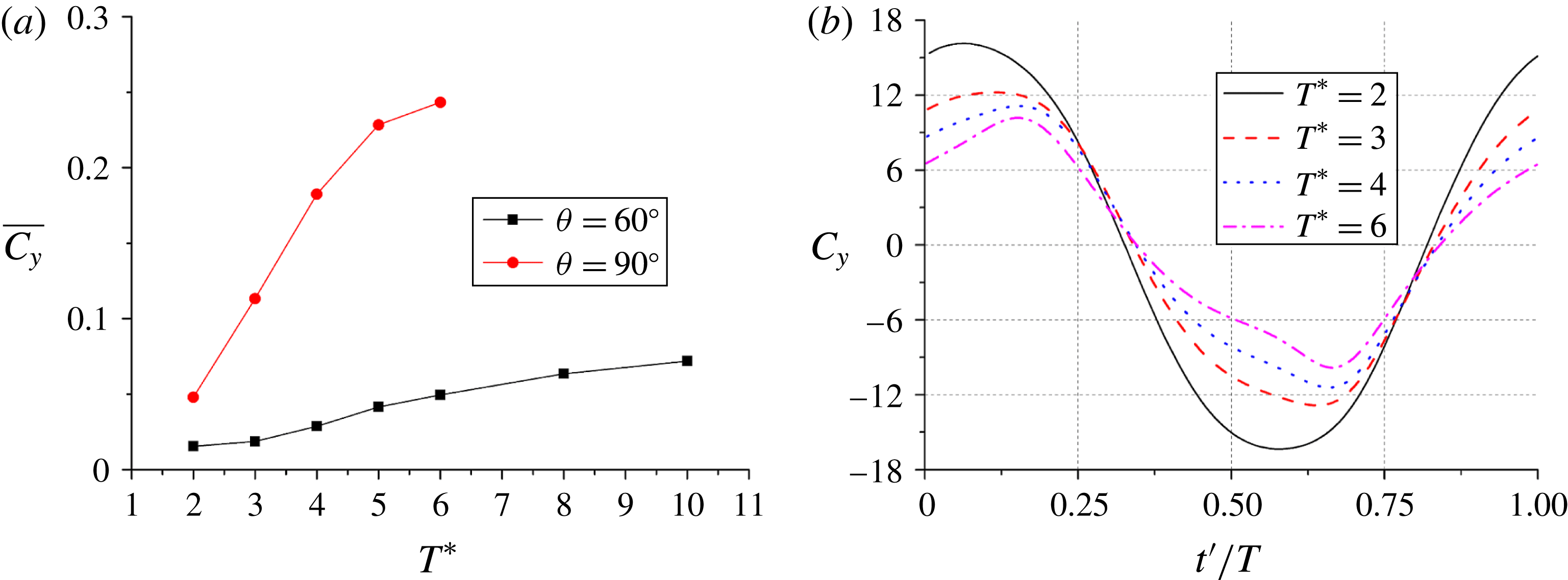
Figure 9(a) shows the average vertical force coefficients as a function of dimensionless period for
 ${\it\theta}=60^{\circ }$
and 90° at
 $Re=50$
. For
 ${\it\theta}=90^{\circ }$
, the average force increases with
 $T^{\ast }$
for
 $T^{\ast }\leqslant 6$
and the flow eventually becomes unstable for
 $T^{\ast }=8$
, whose average force before the flow transition takes place is close to that for
 $T^{\ast }=6$
. The instantaneous force coefficients in one period for
 ${\it\theta}=90^{\circ }$
and
 $T^{\ast }=2{-}6$
are plotted in figure 9(b). The effect of the period is similar to that of the Reynolds number. The curves are more distorted as the period increases, indicating that the effect of the vortices on the average force increases with the period, which is not surprising since the vortices can develop stronger for a longer time before saturation. The added mass force on the body becomes smaller for a larger period due to smaller acceleration, which is responsible for the smaller instantaneous force magnitude for a larger period in figure 9(b).
(a) Evolution of the period-averaged vertical force coefficient, and (b) the instantaneous force coefficients in the 17th, 33rd, 34th and 39th periods which are marked with symbol ‘
 $+$
’ in (a).
 $Re=125$
,
 ${\it\theta}=90^{\circ }$
,
 ${\it\varphi}_{0}=0$
, and
 $T^{\ast }=4$
.

Velocity vectors and vorticity contours in the 16th period at (a)
 $t=15.25T$
, (b)
 $t=15.5T$
, (c)
 $t=15.75T$
and (d)
 $t=16T$
for
 $Re=125$
,
 ${\it\theta}=90^{\circ }$
and
 $T^{\ast }=4$
.

3.1.2. Unstable flow regime
The behaviour of the vertical force for the unstable regime is analysed with the case of
 $Re=125$
,
 ${\it\theta}=90^{\circ }$
and
 $T^{\ast }=4$
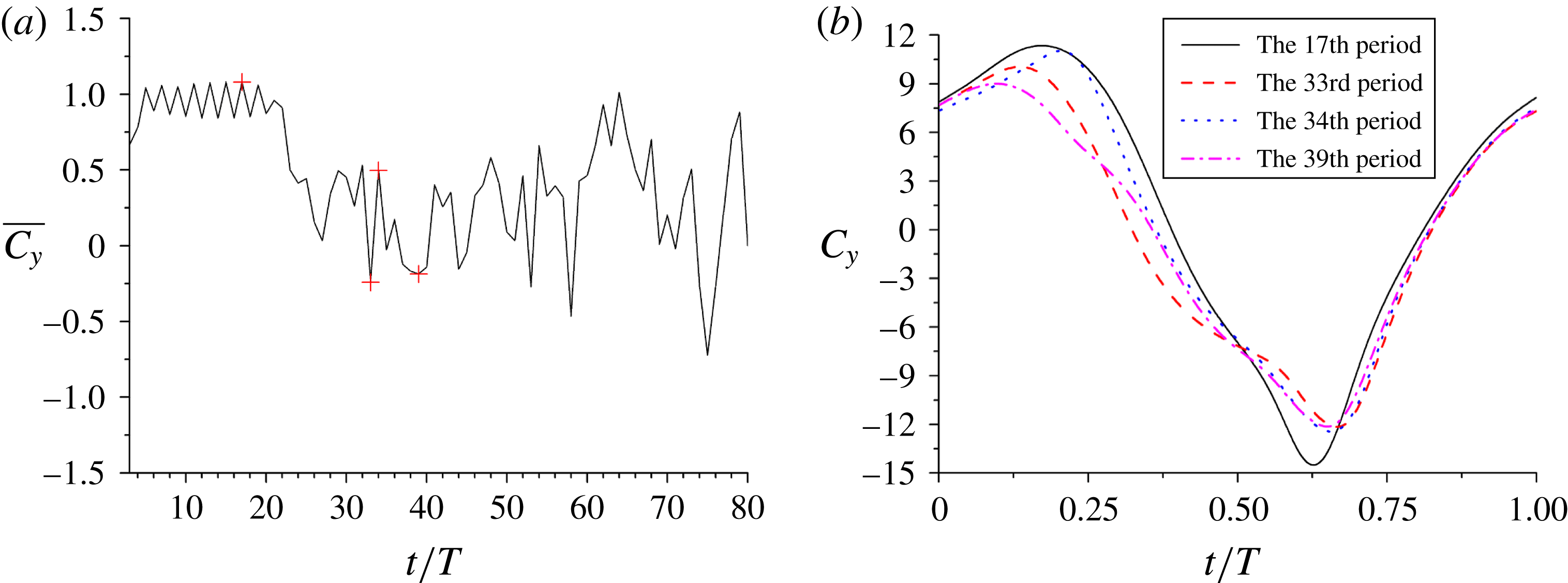
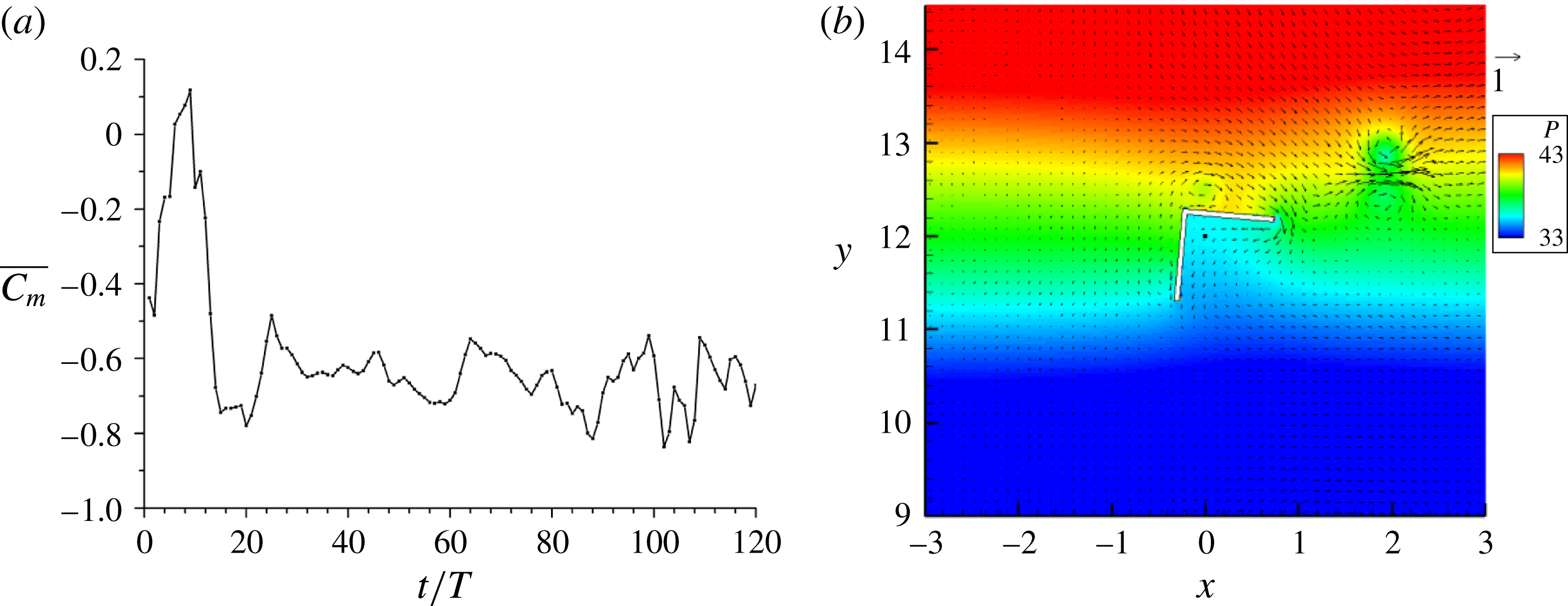
. The evolution of the period-averaged vertical force coefficient for this case is plotted in figure 10(a). The force behaves differently in two stages: keeping a large positive value for
 $t<20T$
and fluctuating irregularly for
 $t>20T$
. After checking the flow fields, we find that in the first stage the flow structures remain symmetrical, as shown in figure 11. Compared to the case of
 $Re=50$
discussed earlier, the shed vortices are stronger and more significantly affect the subsequent reversing flow. For example, the vortex that is shed during upward flow is emitted from each body edge together with the newly-formed vortex as a pair at
 $t^{\prime }=0.75T$
(figure 11
c), and the vortex pairs further influence the subsequent upward flow when they are entrained upward, evidenced by their intensities at
 $t^{\prime }=0.25T$
(figure 11
a or 12
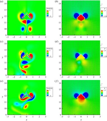
a). In the first stage, though keeping left–right symmetry, the flow is not perfectly periodic. There is a small fluctuation in the average vertical force in figure 10(a) and, accordingly, the shapes of the first vortex pair below the body appear differently at
 $t=15.25T$
(vorticity extended in figure 11
a) and
 $t=16.25T$
(vorticity concentrated in figure 12
a). In the second stage, the flow structures lose the left–right symmetry (figure 12
c,e). The vortices are shed and emitted asymmetrically, and their subsequent motions are irregular, which leads to the irregular fluctuation of the vertical force. The evolutions of vortices during
 $t=15T{-}40T$
are shown in movie 1 available online at http://dx.doi.org/10.1017/jfm.2015.703.
Vorticity contours at (a)
 $t=16.25T$
, (c)
 $t=32.25T$
, (e)
 $t=33.25T$
, and velocity vectors and pressure contours at (b)
 $t=16.25T$
, (d)
 $t=32.25T$
, (f)
 $t=33.25T$
for
 $Re=125$
,
 ${\it\theta}=90^{\circ }$
and
 $T^{\ast }=4$
.

In order to elucidate more clearly the reason for the fluctuation in the average force, the instantaneous force coefficients in the 17th, 33rd, 34th and 39th periods are shown in figure 10(b). Note that the 17th period means
 $t=16T{-}17T$
. From figure 10(a) in which these four periods are marked with symbol ‘
 $+$
’, the force is positive for the 17th and 34th periods and negative for the 33rd and 39th periods. From figure 10(b), the differences in the average forces for these periods can be mainly attributed to the differences in the instantaneous forces during upward flow (i.e.
 $t^{\prime }=0{-}0.5T$
). The forces at
 $t^{\prime }=0.25T$
for the 17th and 34th periods are significantly larger than those for the 33rd and 39th periods. Thus, we plot the vorticity, velocity and pressure fields at
 $t^{\prime }=0.25T$
in the 17th, 33rd and 34th periods (i.e.
 $t=16.25T$
,
 $t=32.25T$
and
 $t=33.25T$
) for comparison in figure 12. At
 $t=16.25T$
and
 $33.25T$
, the first vortex pair below the body produces a jet toward the body, respectively, resulting in relatively high pressure on the bottom sides of the body, whereas at
 $t=32.25T$
, the pair produces a jet in the horizontal direction, resulting in a relatively low pressure on the body, as shown in figure 12. For the stable flow regime, the body can always utilize the vortices to enhance the lift, whereas for the unstable flow regime, the vortices cannot be always utilized due to their irregular motion and may result in the negative lift sometimes. From figure 10(a), we see that the positive force predominates and therefore we think that the vortex-induced lift is still responsible for the lift-enhancement for the hovering pyramid of Weathers et al. (Reference Weathers, Folie, Liu, Childress and Zhang2010).
3.2. Torque coefficient
In the following, we analyse the behaviour of the torque on the body for the stable and unstable flow regimes, respectively.
3.2.1. Stable flow regime
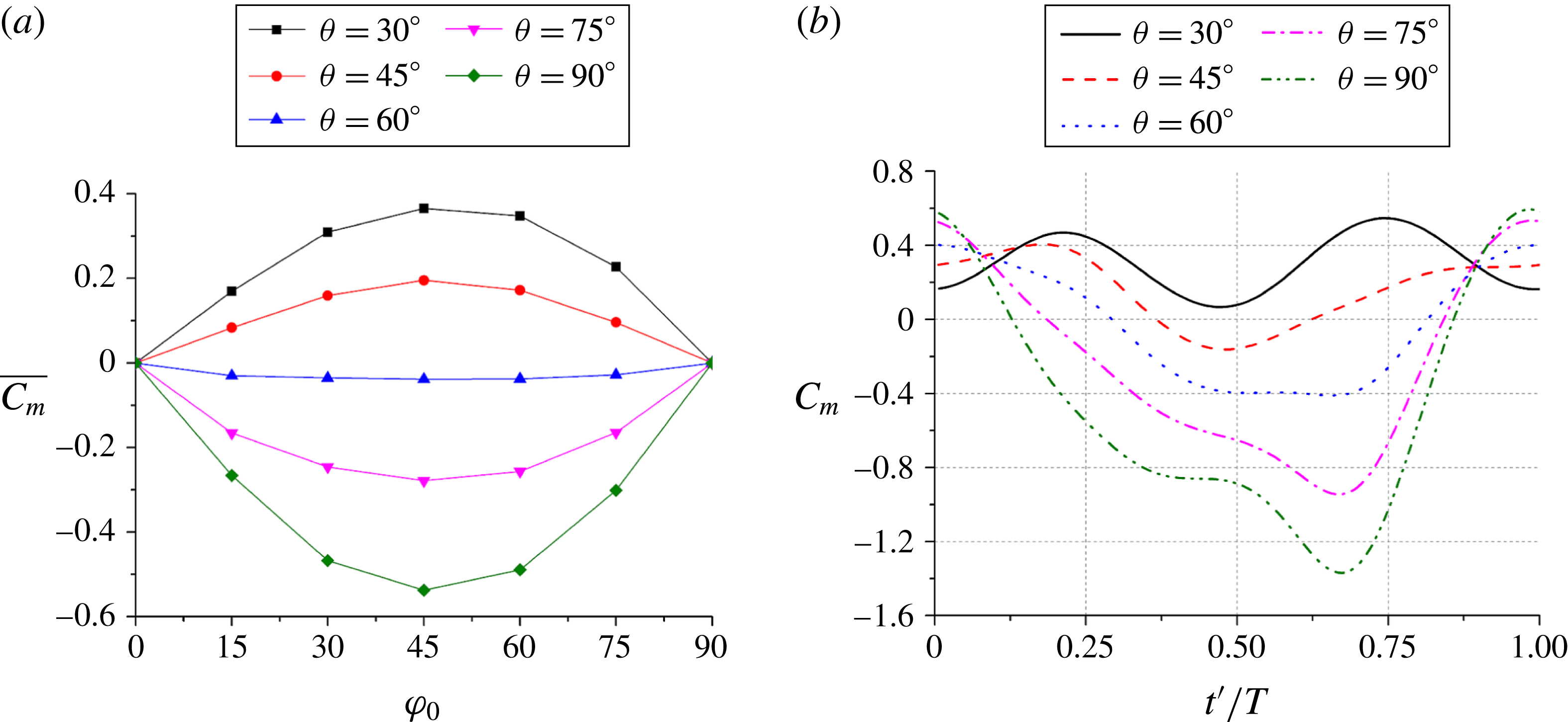
Figure 13(a) shows the average torque coefficients for
 ${\it\theta}=30^{\circ }{-}90^{\circ }$
and
 ${\it\varphi}_{0}=15^{\circ }{-}75^{\circ }$
at
 $Re=50$
and
 $T^{\ast }=2$
. Note that for our definition in figure 1 and a positive tilt angle
 ${\it\varphi}_{0}$
, a negative torque helps the body to return to the upright orientation and is thus called a restoring torque. Similarly, a positive torque is called a destructive torque. From figure 13(a), the body experiences a restoring torque for
 ${\it\theta}=60^{\circ }$
, 75° and 90°, and a destructive torque for
 ${\it\theta}=30^{\circ }$
and 45°, irrespective of the value of tilt angle. The torque magnitude is small for
 ${\it\theta}=60^{\circ }$
, and therefore the critical vertex angle should be close to (and smaller than) 60°. Roughly speaking, the body turns its longer dimension perpendicular to the flow direction, as a non-spherical body settling in a Newtonian fluid (Joseph & Liu Reference Joseph and Liu1993) and a dimer in the oscillatory flow (Wright et al.
Reference Wright, Swift and King2008). In addition, for a fixed vertex angle, the torque magnitude is largest at roughly
 ${\it\varphi}_{0}=45^{\circ }$
and decreases as the tilt angle increases from 45° to 90° or decreases from 45° to 0°, as shown in figure 13(a). This observation may be understood by considering that the body for
 ${\it\varphi}_{0}=0^{\circ }$
or
 ${\it\varphi}_{0}=90^{\circ }$
has the left–right or up–down symmetry and is thus subject to zero average torque.
(a) Average torque coefficients for different tilt and vertex angles and (b) instantaneous torque coefficients in one period for
 ${\it\varphi}_{0}=30^{\circ }$
and different vertex angles.
 $Re=50$
,
 $T^{\ast }=2$
.

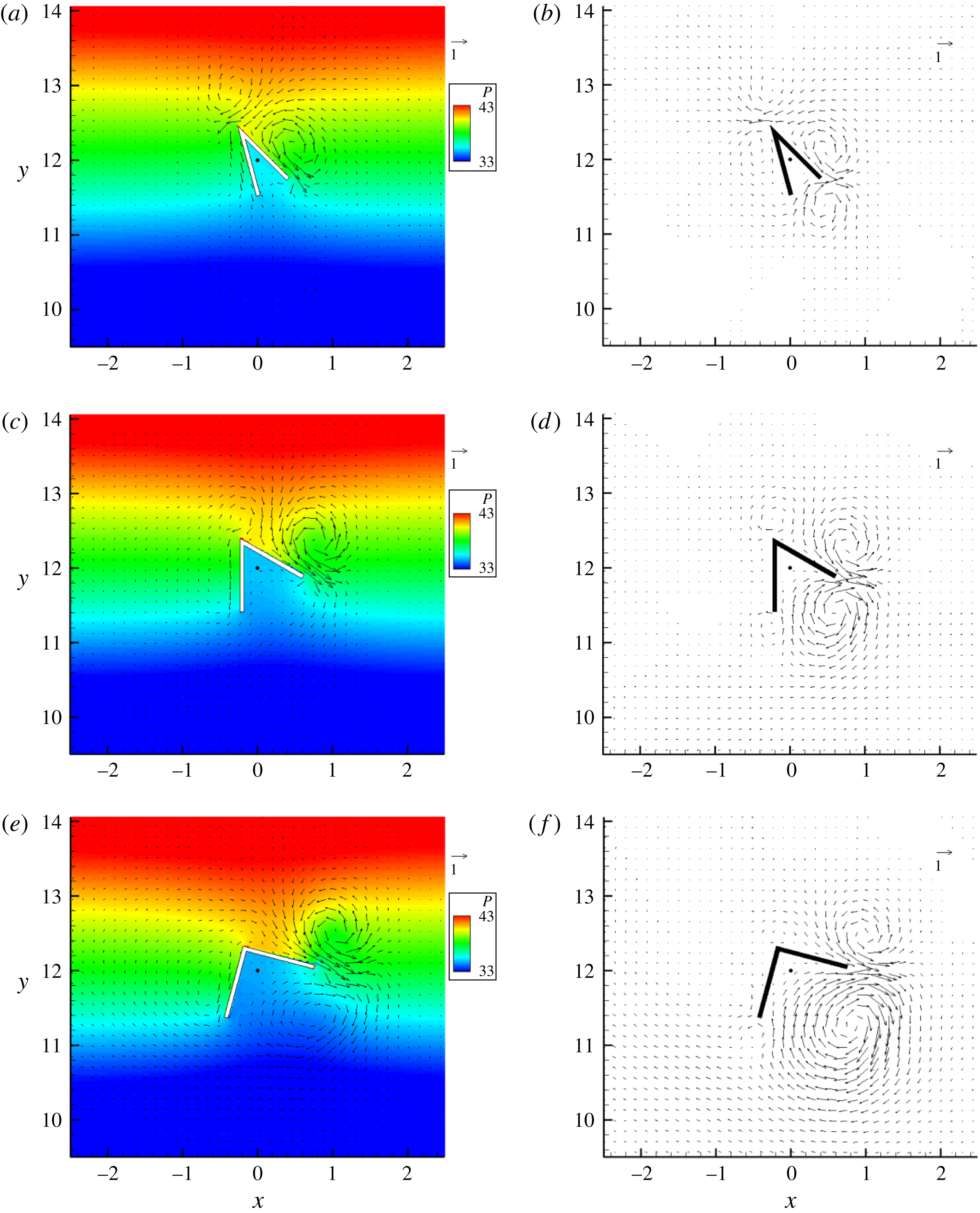
Pressure contours and velocity vectors for (a)
 ${\it\theta}=30^{\circ }$
, (c)
 ${\it\theta}=60^{\circ }$
, (e)
 ${\it\theta}=90^{\circ }$
at
 $t^{\prime }=0.5T$
and average velocity vectors for (b)
 ${\it\theta}=30^{\circ }$
, (d)
 ${\it\theta}=60^{\circ }$
, (f)
 ${\it\theta}=90^{\circ }$
. The black point represents the body’s mass centre.
 $Re=50$
,
 $T^{\ast }=2$
, and
 ${\it\varphi}_{0}=30^{\circ }$
.

The instantaneous torque coefficients in one period for
 ${\it\theta}=30^{\circ }{-}90^{\circ }$
at
 ${\it\varphi}_{0}=30^{\circ }$
are shown in figure 13(b). The instantaneous torque is always destructive for
 ${\it\theta}=30^{\circ }$
, whereas for
 ${\it\theta}=90^{\circ }$
the instantaneous torque is negative for most time except the time around
 $t^{\prime }=0$
when the upward acceleration of the fluid is large. The differences in the instantaneous torques for different vertex angles are most pronounced during the time interval
 $t^{\prime }=0.25T{-}0.75T$
when the fluid accelerates downward. Therefore, we plot the pressure contours and velocity vectors for
 ${\it\theta}=30^{\circ }$
, 60° and 90° at
 $t^{\prime }=0.5T$
in figure 14(a,c,e). From figure 14, the torque is mainly caused by the pressure difference on the right edge. We see two reasons for the destructive torque for small vertex angles and the restoring torque for large vertex angles, corresponding to two factors for the torque: the force and the position of the mass centre. Regarding the force, for
 ${\it\theta}=30^{\circ }$
a pair of vortices induce a jet toward the body vertex, resulting in large pressure at the vertex area, as shown in figure 14(a), whereas for
 ${\it\theta}=90^{\circ }$
, the vortex near the vertex existing for
 ${\it\theta}=30^{\circ }$
disappears, and the other vortex moves to the edge tip, resulting in the high pressure distribution extended toward the edge tip, as shown in figure 14(e). Regarding the position of the mass centre, the projection point of the body mass centre on the right edge along the perpendicular direction is shifted closer to the vertex as the vertex angle increases, as can be seen in figure 14 where the mass centre is marked by a black point. It can be estimated that the distance between this projection point and the vertex is around
 $a\cos ^{2}({\it\theta}/2)/2$
, which decreases with increasing
 ${\it\theta}$
. Clearly, these two effects can explain the destructive torque for small vertex angles and the restoring torque for large vertex angles. The effect of the position of the body mass centre on the hovering stability was demonstrated by Liu et al. (Reference Liu, Ristroph, Weathers, Childress and Zhang2012), who enhanced the hovering stability of the pyramid by adding additional weight to the top of the body.
The period-averaged velocity fields for
 ${\it\theta}=30^{\circ }$
, 60° and 90° at
 ${\it\varphi}_{0}=30^{\circ }$
and
 $Re=50$
are shown in figure 14(b,d,f). Generally, the vortex pair and corresponding jet form at the body points protruding laterally most into fluids, e.g. the vertex and the tip of the right edge for
 ${\it\theta}=30^{\circ }$
and two edge tips for
 ${\it\theta}=90^{\circ }$
. The vortex pair is stronger if the corresponding edge is aligned closer to the horizontal direction. As an example, for
 ${\it\theta}=90^{\circ }$
and
 ${\it\varphi}_{0}=30^{\circ }$
, the vortex pair for the right edge is much stronger than the other pair in figure 14(f).
3.2.2. Unstable flow regime
Liu et al. (Reference Liu, Ristroph, Weathers, Childress and Zhang2012) conducted a visualization experiment on the flow structures produced by a
 $\wedge$
-shaped body in an oscillating flow and observed that the vortex dipole produced on the edge aligned closer to the horizontal direction was emitted sideways (in the direction roughly perpendicular to the body’s axis of symmetry) and the other dipole was weak. From this observation, they suggested a mechanism for the stable hovering: the jet from the vortex dipole emitted sideways produces a restoring torque for a tilted body. This observation is reproduced in our simulations for
 $Re=250$
,
 $T^{\ast }=2$
,
 ${\it\theta}=90^{\circ }$
and
 ${\it\varphi}_{0}=40^{\circ }$
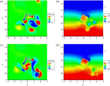
. The vortex pair and the lateral jet can be seen in figure 15(b), which shows the pressure contours and velocity vectors at
 $t^{\prime }=0.5T$
. Unlike the case of
 ${\it\varphi}_{0}=0^{\circ }$
where the pair is emitted at
 $t^{\prime }=0.75T$
during downward flow (figure 11
c), the pair for
 ${\it\varphi}_{0}=40^{\circ }$
is emitted at
 $t^{\prime }=0.25T$
during upward flow and therefore it moves laterally and slightly upward (in the direction roughly perpendicular to the body axis of symmetry), as in the experiment (their figure 2) of Liu et al. (Reference Liu, Ristroph, Weathers, Childress and Zhang2012). Movie 2 shows the persistent leftward ejections of the vortex pairs. The jet produces high pressure over the upper side of the edge (figure 15
b) and a persistent restoring torque, as shown in figure 15(a).
(a) Evolutions of the period-averaged torque coefficient and (b) the pressure contours and velocity vectors at
 $t=49.5T$
for
 $Re=250$
,
 ${\it\theta}=90^{\circ }$
,
 ${\it\varphi}_{0}=40^{\circ }$
and
 $T^{\ast }=2$
.

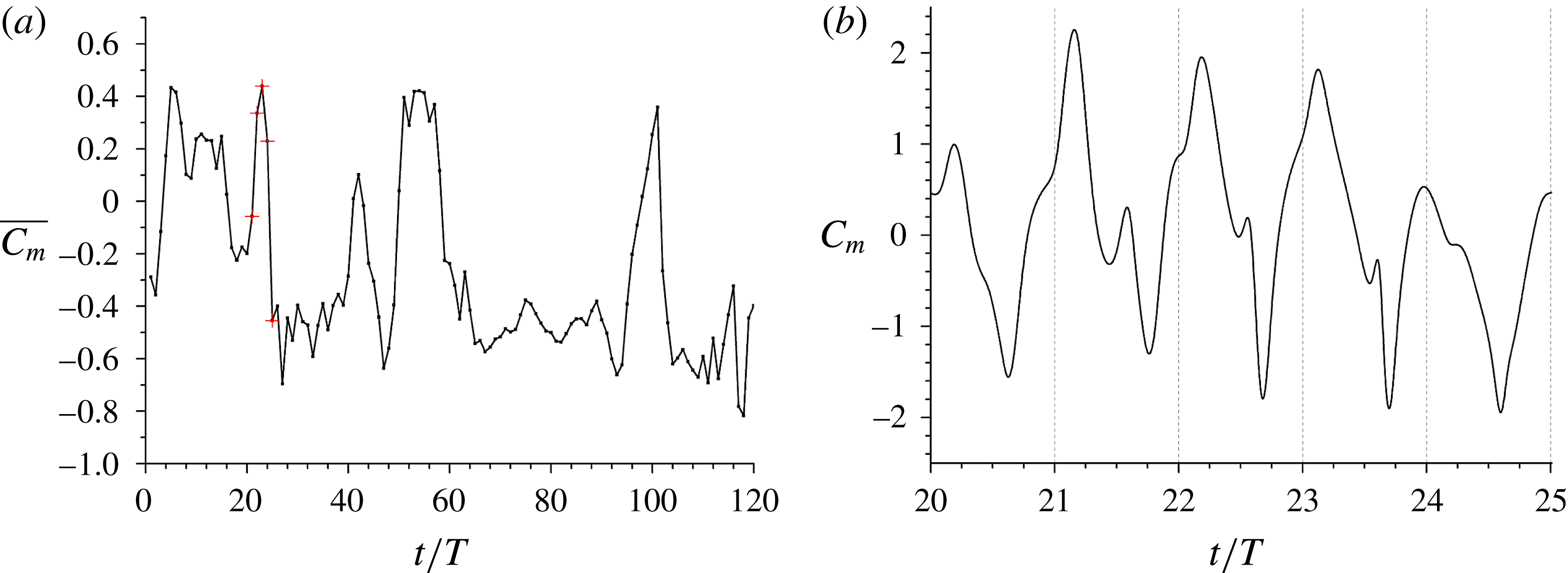
We next discuss the results for a relatively small tilt angle. The evolution of the period-averaged torque coefficient for
 $Re=250$
,
 $T^{\ast }=2$
,
 ${\it\theta}=90^{\circ }$
and
 ${\it\varphi}_{0}=20^{\circ }$
is shown in figure 16(a). The average torque cannot always keep being negative and sometimes jumps to be positive, similar to the behaviour of the force in the unstable regime discussed earlier. Figure 16(b) plots the instantaneous torque coefficient from
 $t=20$
to
 $t=25$
. The period-averaged torques are negative for the 21st and 25th periods and positive for the 22nd–24th periods, as marked in figure 16(a). The instantaneous torque in the 21st and 25th periods changes roughly in phase with the fluid acceleration, as in the stable regime for
 ${\it\theta}\geqslant 60^{\circ }$
(figure 13
b). By contrast, there is a pronounced positive peak between
 $t^{\prime }=0$
and
 $t^{\prime }=0.25T$
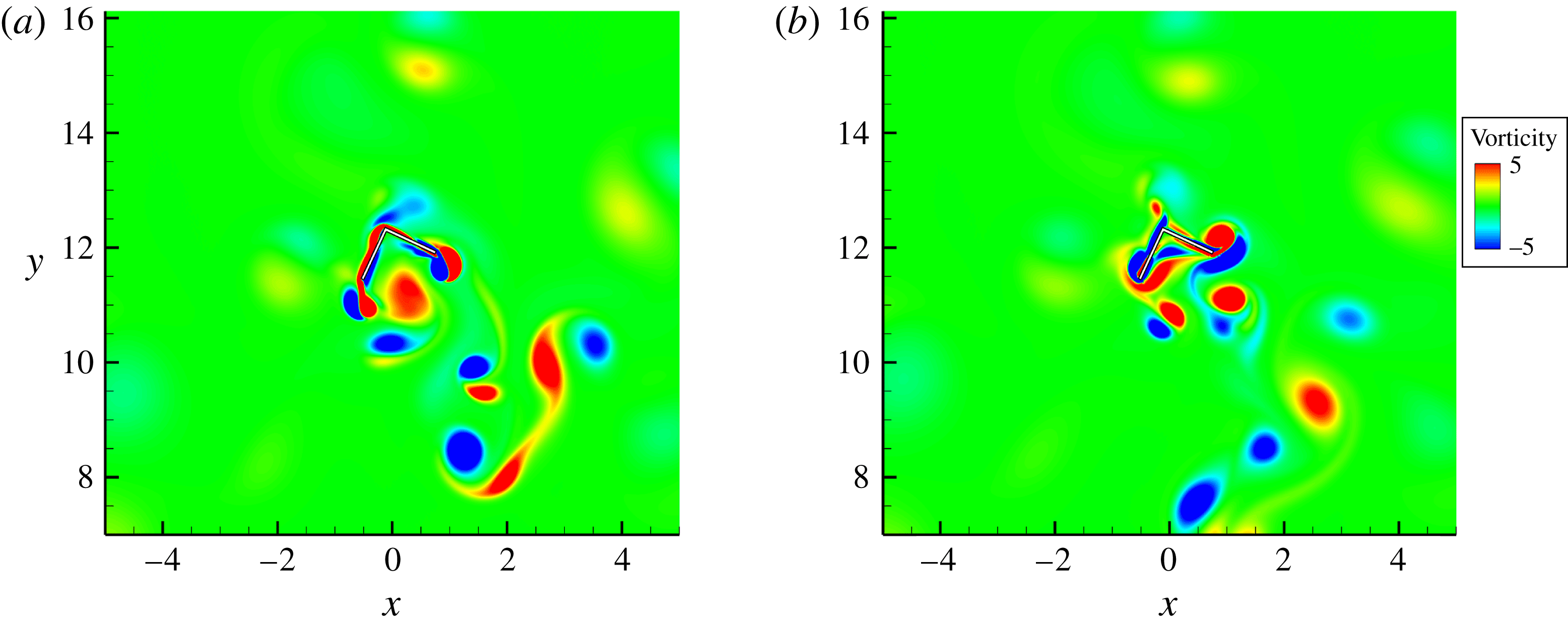
for the 22nd–24th periods, respectively, which renders the average torque positive. The vorticity contours, pressure contours and velocity vectors at
 $t=20.125T$
and
 $t=21.125T$
are shown in figure 17. We see that at
 $t=21.125T$
two counter-clockwise rotating vortices (in red color online) below the body are merging into a strong vortex, inducing a flow toward the right edge, and causing higher pressure on the bottom side of the right edge and thereby a bigger positive instantaneous torque, compared to the situation at
 $t=20.125T$
. From our animation (see supplementary movie 3), one of two merging vortices at
 $t=21.125T$
in figure 17(c) comes from the one in red located at the bottom at
 $t=20.125T$
in figure 17(a), and the merged vortex exists below the body for over 2 periods with the new vortex shed on the left edge joining in each period, as shown in figure 18(a) at
 $t=23.75T$
. Therefore, we think that this vortex is mainly responsible for the pronounced positive torque peaks in the 22nd–24th periods. For the 25th period, the instantaneous torque has no such positive peak (figure 16
b) and the average restoring torque is large (figure 16
a). This result can be explained by the fact that the aforementioned strong counter-clockwise rotating vortex immediately below the body is absent (see supplementary movie 3). In addition, we observe in supplementary movie 3 that generally the downward emission of a vortex pair predominates during periods with the destructive torque, and the lateral emission of a vortex pair at
 $t^{\prime }=0.25T$
(figure 18
b) predominates during periods with the restoring torque. Considering that the aforementioned strong counter-clockwise rotating vortex also forms by merging the vortices emitted downward, the emission direction of the vortex pair is most crucial to the direction of the torque. Movie 4 shows the persistent lateral emission of the vortex pairs for
 ${\it\varphi}_{0}=20^{\circ }$
during
 $t=70T{-}80T$
when the restoring torque prevails (figure 16
a).
(a) Evolutions of the period-averaged torque coefficient and (b) instantaneous torque coefficient from
 $t=20$
to
 $t=25$
for
 $Re=250$
,
 ${\it\theta}=90^{\circ }$
,
 ${\it\varphi}_{0}=20^{\circ }$
and
 $T^{\ast }=2$
.

Vorticity contours at (a)
 $t=20.125T$
and (c)
 $t=21.125T$
, and pressure contours and velocity vectors at (b)
 $t=20.125T$
and (d)
 $t=21.125T$
for
 $Re=250$
,
 ${\it\theta}=90^{\circ }$
,
 ${\it\varphi}_{0}=20^{\circ }$
and
 $T^{\ast }=2$
.

Vorticity contours at (a)
 $t=23.75T$
and (b)
 $t=25.25T$
for
 $Re=250$
,
 ${\it\theta}=90^{\circ }$
,
 ${\it\varphi}_{0}=20^{\circ }$
and
 $T^{\ast }=2$
.

It is expected that the lateral emission of the vortex pair prevails over the downward emission more significantly when the tilt angle of the body becomes larger and takes place persistently for each period when the body edge is aligned close to the horizontal direction, as observed for
 ${\it\varphi}_{0}=40^{\circ }$
. The destructive effect of the vortices emitted downward for a small tilt angle (e.g. figure 17
c) may explain why a big tilt angle such as 50° was frequently reached for the hollow pyramid in the experiments (Weathers et al.
Reference Weathers, Folie, Liu, Childress and Zhang2010; Liu et al.
Reference Liu, Ristroph, Weathers, Childress and Zhang2012). The lateral ejection of the vortex pair at big tilt angles then prevents the body from overturning.
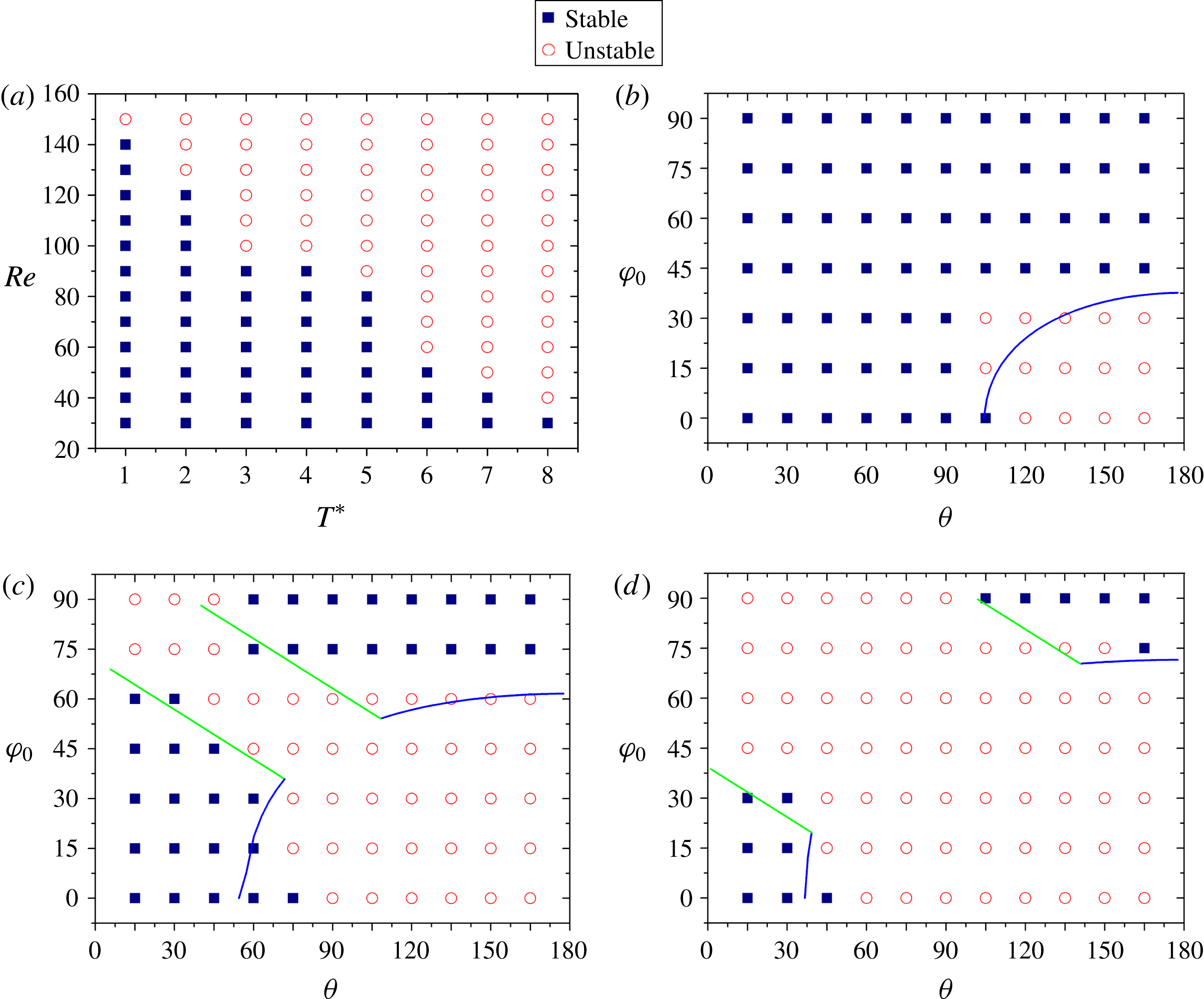
Phase diagrams for the stable and unstable flow regimes in (a)
 $(Re,T^{\ast })$
space at
 ${\it\theta}=90^{\circ }$
and
 ${\it\varphi}_{0}=0^{\circ }$
, (b)
 $({\it\theta},{\it\varphi}_{0})$
space at Re
 $=$
60 and
 $T^{\ast }=4$
, (c)
 $({\it\theta},{\it\varphi}_{0})$
space at
 $Re=100$
and
 $T^{\ast }=4$
, and (d)
 $({\it\theta},{\it\varphi}_{0})$
space at
 $Re=150$
. The lines in (b,c,d) represent the solutions to
 $Re_{s}=95$
and (3.1)–(3.3).

3.3. Effects of the parameters on the flow transition
After illustrating the significantly different dynamics in the stable and unstable flow regimes, we now examine how the parameters affect the flow transition from the stable regime to the unstable one. There are four control parameters: Reynolds number
 $Re$
, dimensionless period
 $T^{\ast }$
, vertex angle
 ${\it\theta}$
, and tilt angle
 ${\it\varphi}_{0}$
. Figure 19(a) shows the phase diagram for the stability of the flow in the
 $(Re,T^{\ast })$
space at
 ${\it\theta}=90^{\circ }$
and
 ${\it\varphi}_{0}=0^{\circ }$
. Clearly, the increase in the Reynolds number or the dimensionless period can lead to the flow transition from the stable state to the unstable one. Figure 19(b–d) plots the phase diagrams in the
 $({\it\theta},{\it\varphi}_{0})$
space for
 $Re=60$
, 100 and 150, respectively, with
 $T^{\ast }=4$
. For all three Reynolds numbers, the flows are stable when the vertex and tilt angles are both small, or large, either of which corresponds to small body span in the horizontal direction. Therefore, the Reynolds number based on the body span is expected to be an important parameter for the flow transition, recalling that our
 $Re$
is based on the side length of the body
 $a$
. The body span
 $s$
can be determined from
 $a$
,
 ${\it\theta}$
and
 ${\it\varphi}_{0}$
:
 $$\begin{eqnarray}\displaystyle & \displaystyle s=2a\sin ({\it\theta}/2)\cos ({\it\varphi}_{0})\quad \text{for }{\it\varphi}_{0}\leqslant {\it\theta}/2, & \displaystyle\end{eqnarray}$$
 $$\begin{eqnarray}\displaystyle & \displaystyle s=a\sin ({\it\theta}/2+{\it\varphi}_{0})\quad \text{for }{\it\varphi}_{0}\geqslant {\it\theta}/2. & \displaystyle\end{eqnarray}$$
 ${\it\varphi}_{0}={\it\theta}/2$
. The body span is equal to the projected length of the virtual baseline for
 ${\it\varphi}_{0}<{\it\theta}/2$
and that of the right edge for
 ${\it\varphi}_{0}>{\it\theta}/2$
. We define the Reynolds number based on the body span as
 $Re_{s}={\it\rho}_{f}v_{A}s/{\it\mu}$
. Clearly,
 $$\begin{eqnarray}Re_{s}=(s/a)Re.\end{eqnarray}$$
 $Re_{s}$
is a function of the vertex and tilt angles for a given
 $Re$
. In Figure 19(b–d), we plot the curves satisfying
 $Re_{s}=95$
and (3.1)–(3.3). The blue and green lines represent the branches of
 ${\it\varphi}_{0}\leqslant {\it\theta}/2$
(3.1) and
 ${\it\varphi}_{0}\geqslant {\it\theta}/2$
(3.2), respectively. It is observed that these curves for constant
 $Re_{s}$
overall agree with the results from the simulations, indicating that the flow transition mainly depends on the Reynolds number based on the body span for a given dimensionless period. Nevertheless, the orientation of the body also affects the flow stability, or the critical
 $Re_{s}$
. For a given body span, the flow is relatively more stable for
 ${\it\varphi}_{0}=0$
(a symmetrical configuration), as implied from the observation that there are stable points on the right side of the curves for
 ${\it\varphi}_{0}=0$
in figure 19(b–d), and relatively less stable when the left edge aligns vertically and the right edge tilts upward, since there are unstable points above the curves near the upper intersection points in figure 19(c,d). The reason for the effect of the body orientation on the flow stability is not clear, and may involve the subtle effect of the edge tip.
3.4. Freely moving body
Our results on the fixed body predict the stable orientation for a hovering body in the stable flow regime and irregular motion in the unstable regime. The aim of this sub-section is to simply demonstrate these predictions. From the value of the body-to-fluid mass ratio
 $m/{\it\rho}_{f}L_{p}^{3}\sim 10$
in the experiment of Liu et al. (Reference Liu, Ristroph, Weathers, Childress and Zhang2012), where
 $m$
and
 $L_{p}$
are the pyramid mass and height, respectively, we set
 ${\it\rho}_{r}=80$
for our two-dimensional open triangle so that our body-to-fluid mass ratio
 $(m/{\it\rho}_{f}a^{2}\approx {\it\rho}_{s}2ah/{\it\rho}_{f}a^{2}=2{\it\rho}_{r}h/a)$
is around 10. For the stable regime,
 $Re=50$
and
 $T^{\ast }=2$
. We consider three vertex angles:
 ${\it\theta}=30^{\circ }$
, 60° and 90°. For
 ${\it\theta}=30^{\circ }$
, the horizontal orientation and zero average vertical force are expected at the terminal stable state, and thus the gravity effect is not considered. For
 ${\it\theta}=60^{\circ }$
and 90°, the Froude number, defined as
 $Fr=ga/v_{A}^{2}$
, is
 $8.2\times 10^{-4}$
and
 $2.53\times 10^{-3}$
, respectively, from the balance between the buoyant force and the average vertical force, namely,
 ${\it\rho}_{f}S_{P}g({\it\rho}_{r}-1)=\bar{C}_{y}{\it\rho}_{f}v_{A}^{2}a/2$
, where the force coefficient
 $\bar{C}_{y}$
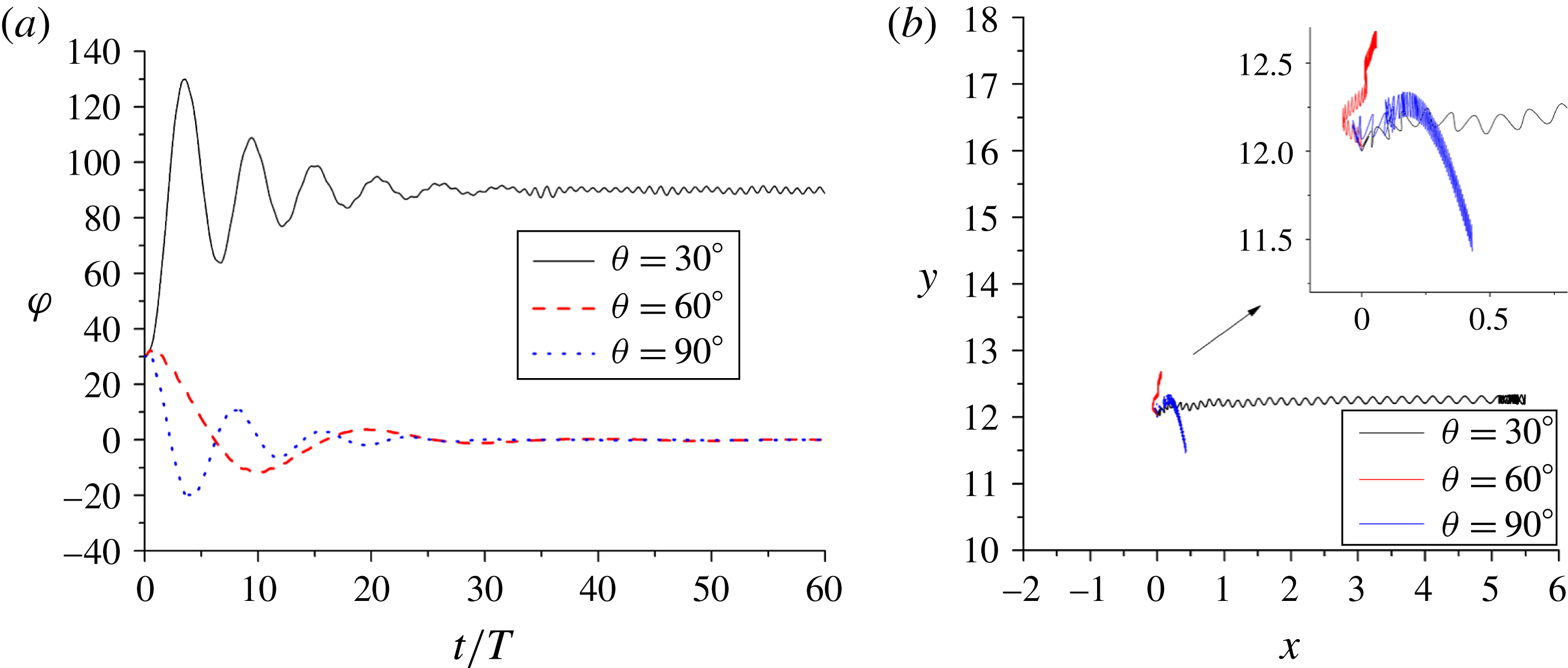
is obtained from the result for a fixed upright body in figure 9(a). The evolutions of the tilt angles and the trajectories of the bodies released at the center of the computational domain with the initial tilt angle of 30° for
 ${\it\theta}=30^{\circ }$
, 60° and 90° during
 $t=0{-}60T$
are shown in figure 20. As expected, the bodies for
 ${\it\theta}=60^{\circ }$
and 90° turn to the upright orientation and the body for
 ${\it\theta}=30^{\circ }$
turns to the horizontal orientation. The body tilt angles for all cases undergo several pronounced oscillations before reaching the stable states as a result of large body inertia. The body vertical velocities for
 ${\it\theta}=60^{\circ }$
and 90° are very small, evidenced by the small distances the bodies travel during 60 time periods in figure 20(b). The vertical oscillations in the trajectories due to the oscillating flow are clear in the insert of figure 20(b). It is interesting that the body for
 ${\it\theta}=30^{\circ }$
migrates rapidly rightward, namely the body-shape-diverging direction, until the body collides with the right boundary at around
 $t=35T$
(keeping colliding afterwards). By contrast, Wright et al. (Reference Wright, Swift and King2008) observed that an asymmetric dimer comprising a pair of spheres of unequal size migrated along the body-shape-converging direction. The reason for the disparity is that our body is hollow and open, and the pressure on the outer sides of the edges which are only upwinding surfaces in the up–down oscillating flow produces a force with the
 $x$
-component pointing toward the body-shape-diverging direction, whereas the big sphere of Wright et al. (Reference Wright, Swift and King2008) had an upwinding surface on which the pressure had the
 $x$
-component pointing toward the body-shape-converging direction.
Figure 21 shows the evolutions of the tilt angles and the trajectories of the body for
 $Re=250$
,
 ${\it\theta}=90^{\circ }$
,
 $T^{\ast }=2$
and
 $Fr=5.85\times 10^{-3}$
. As expected, we observe the irregular oscillation of the tilt angle, frequent occurrence of large tilt angles and no overturning of the body. The motion of the body and the evolutions of the vortices before
 $t=40T$
are shown in supplementary movie 5. It is observed that for relatively small tilt angles, the vortex pairs are mainly shed downward, and the vortices randomly entering the region just below the body edges have significant effects on the rotational (destructive toque) and translational (lift force) motions of the body. When a big tilt angle is reached, the lateral ejection of the vortex pair produces a restoring toque on the body. These results are consistent with the observations in the static simulations. Due to the motion of the body, the persistent lateral ejection of vortex pairs is not observed in the dynamics simulations.
Evolutions of the (a) tilt angles and (b) trajectories of the freely moving bodies with the vertex angles
 ${\it\theta}=30^{\circ }$
, 60° and 90° for
 $Re=50$
and
 $T^{\ast }=2$
. The insert in (b) shows the close-up of the trajectories.

Evolutions of the (a) tilt angle and (b) trajectory of the freely moving body for
 ${\it\theta}=90^{\circ }$
,
 $Re=250$
and
 $T^{\ast }=2$
.

4. Conclusion
We have numerically investigated the dynamics of an open triangle in a vertically oscillatory flow for the stable and unstable flow regimes with the DF/FD method. From our results, the following conclusions can be drawn:
Regarding the vertical force on the fixed body with upright orientation:
-
(1) In the stable regime, the steady streaming structure mainly comprises two vortex pairs located respectively above and below the body. Due to up–down asymmetry of the body, the pair below the body produces a larger vertical force on the body than the upper pair, which is the primary reason for the non-zero average force at relatively high Reynolds numbers. The average force increases with increasing Reynolds number or increasing dimensionless period for the parameter range studied, presumably due to the stronger vortex effects for higher Reynolds numbers or larger dimensionless periods.
-
(2) In the unstable regime at relatively high Reynolds numbers, the vortex shed during upward flow is emitted together with the newly-formed vortex as a pair during downward flow for each body edge. The flow structures will lose the left–right symmetry. The vortices are shed and emitted asymmetrically, and their subsequent motions are irregular, which leads to the irregular fluctuation of the vertical force. It is observed that the upward jet produced by the vortex pair below the body leads to the positive force, whereas the lateral jet by the pair leads to the negative force.
Regarding the torque on a tilted body:
-
(3) In the stable regime, the body experiences a restoring torque when its vertex angle is larger than a critical value being close to (and smaller than) 60° and otherwise a destructive torque, irrespective of the value of tilt angle, indicating that the body largely turns its longer dimension perpendicular to the flow direction. For a fixed vertex angle, the torque magnitude is largest when the tilt angle is around 45°. The differences in the instantaneous torques for different vertex angles are most pronounced during downward acceleration of the fluid. The reason for the destructive torque for small vertex angles and the restoring torque for large vertex angles is that the pressure force concentrated on the edge is shifted from the vertex toward the edge tip while the projection point of the body mass centre on the edge along the perpendicular direction is shifted closer to the vertex, as the vertex angle increases.
-
(3) In the unstable regime, the persistent ejection of vortex pair during upward flow and corresponding restoring torque are observed for a large tilt angle with one edge aligned close to the horizontal direction, as in the experiment of Liu et al. (Reference Liu, Ristroph, Weathers, Childress and Zhang2012). For a relatively small tilt angle, the emission direction of the vortex pair has intermittency, leading to the intermittency in the direction of torque. A strong counter-clockwise rotating vortex forming from mergence of the vortices emitted downward from both edges is observed to lead to the pronounced instantaneous destructive torque.
-
(3) The predictions on the stable orientation for a hovering body in the stable flow regime and the irregular motion in the unstable regime are confirmed in the dynamic simulation of a freely moving body. The body with the stable horizontal orientation in case of small vertex angle migrates along the body-shape-diverging direction.
In addition, our results indicate that the flow transition from the stable state to the unstable state mainly depends on the Reynolds number based on the body span and the dimensionless period, although the orientation of the body also has a subtle effect.
Acknowledgements
The work was supported by the National Natural Science Foundation of China (grant nos 11372275 and 11132008), Research Fund for the Doctoral Program of Higher Education of China (20130101110035) and the Program for New Century Excellent Talents in University.
Supplementary movies
Supplementary movies are available at http://dx.doi.org/10.1017/jfm.2015.703.