


1. Introduction
During his development of the denotational semantics of System
 $\mathsf {F}$
in the cartesian closed category of qualitative domains, and more specifically of coherence spaces, Girard observed in Girard (Reference Girard1986) that a specific class of morphisms arises naturally among the general morphisms of this model (the stable maps). These particular stable functions are characterized by an additional preservation property: they commute with compatible unions.
Girard not only recognized the relevance of these morphisms to the description of the stable semantics, he also understood that they should play a more fundamental role than the general stable functions themselves. He called them linear maps because they collectively behave very much like linear maps in algebra, forming a symmetric monoidal closed category which is even
 $\ast$
-autonomous (a general categorical notion introduced in Barr (Reference Barr1979) describing categories of linear morphisms where all objects are reflexive, i.e., canonically isomorphic to their bidual).
He understood that this observation, a priori relative to the stable semantics, was the denotational shadow of a fundamental and hitherto hidden structure of Intuitionistic Logic itself: Linear Logic (LL), see Girard (Reference Girard1987). This essential discovery had a major impact in Logic and Computer Science, notably on the study and design of programming languages.
One aspect of linearity which is not directly addressed in LL – although it is contemplated in the concluding section of Girard (Reference Girard1987) — is its central role in the differential calculus where differentiation consists in extracting from a morphism its “best linear approximation”. The purpose of Differential LL (DiLL for short) is to take this role of linearity into account. This logical system was introduced by the author and Laurent Regnier in Ehrhard and Regnier (Reference Ehrhard and Regnier2003, Reference Ehrhard and Regnier2006b) and is summarized in Ehrhard (Reference Ehrhard2018). It extends LL without adding new connectives, but by adding a set of new deduction rules that we can classify as follows.
-
• There are 3 rules relative to the exponential modality
 ${!}\_$
, dual to the standard rules of weakening, contraction, and dereliction.
-
• And there are two rules expressing that any finite family of proofs of the same formula has a sum, which is again a proof of that formula. This includes the case of an empty family, meaning that any formula is provable by a
$0$
proof.


These latter rules mean that the proofs in
 $\mathsf {DiLL}$
are essentially partial: the
 $0$
proof is very similar to the term
 $\Omega$
in the theory of Böhm trees, which is a completely undefined term. More importantly, the unrestricted ability of adding proofs of the same formula means that DiLL features a fundamental nondeterminism in the sense that it is possible to add the two normal proofs of
 ${1}\oplus {1}$
, which corresponds to the type of booleans, that is, intuitively, the two booleans
 $\mathbf t$
and
 $\mathbf f$
. The most natural operational understanding of this “boolean”
 $\mathbf t+\mathbf f:{1}\oplus {1}$
consists in considering it as a program, which can nondeterministically reduce to
 $\mathbf t$
or
 $\mathbf f$
. We provide in Section 3.2 a more precise description of the
 $\lambda$
-calculus account of this extension of LL, which features a typing rule allowing one to add any two terms having the same type.
1.1 Determinism and differentiation
In Ehrhard and Regnier (Reference Ehrhard and Regnier2008, Reference Ehrhard, Regnier, Beckmann, Berger, Löwe and Tucker2006a), we developed a Taylor expansion of
 $\lambda$
-terms, which is based on the differential
 $\lambda$
-calculus. This expansion consists in translating a
 $\lambda$
-term
 $M$
into a (generally infinite) sum
 $M^\ast$
of “resource terms,” that is, of differential
 $\lambda$
-terms whose only use of the standard
 $\lambda$
-calculus operation of application is application to
 $0$
. In other words, all the applications
 $({P}){Q}$
are replaced hereditarily by differential terms:
 \begin{align*} (({P}){Q})^\ast = \sum _{n=0}^\infty \frac 1{{n}!} ({{\mathsf{D}}^nP^\ast \cdot (\overbrace {Q^\ast ,\ldots ,Q^\ast }^n)}){0}\,. \end{align*}
In this expression, if
 $M:{A}\Rightarrow {B}$
and
 $N_1,\ldots ,N_n:A$
are differential
 $\lambda$
-term, then
 \begin{equation*}{\mathsf{D}}^nM\cdot (N_1,\ldots ,N_n):{A}\Rightarrow {B}\end{equation*}
is the
 $n$
th derivative of
 $M$
applied to linear argument
 $N_{1},\ldots ,N_{n}$
, see Section 3.2.
Analyzing the execution of standard
 $\lambda$
-terms in the Krivine Machine we showed that, if a standard
 $\lambda$
-term
 $M$
is
 $\beta$
-equivalent to a variable
 $x$
then there is exactly one term
 $s$
in the Taylor expansion
 $M^\ast$
of
 $M$
which does not reduce to
 $0$
, and
 $s$
reduces to
 $({M^\ast _s})^{-1}\,x$
, if we take multiplicities into account.Footnote
1
This resource term
 $s$
is a trace of the execution of
 $M$
in the machine, or more precisely,
 $s$
provides a precise account of the quantitative use of the various subterms of
 $M$
during the execution.
In other words, in the infinite sum
 $M^\ast$
, only one term is nonzero, although for knowing which one, one needs to reduce
 $M$
to its normal form. This means that this infinite sum is only apparently nondeterministic. But for proving this property, we strongly use the fact that
 $M$
is a standard
 $\lambda$
-term, that is, contains no differential construct of shape
 ${\mathsf{D}} P\cdot Q$
.
So beyond this first encouraging observation, the question remained open of whether differentiation (in the sense of
 $\mathsf {DiLL}$
) can be made compatible with determinism. Toward a positive answer to this question, the second crucial observation was that, in the model of LL based on probabilistic coherence spaces (PCSs), nonlinear morphisms are functions which are analytic in the sense that they are defined by power series and hence should be differentiable, in spite of the fact that, in the corresponding category
 $\mathbf{Pcoh}$
, it is not always possible to add two morphisms of the same type. For instance, the sum of two subprobability distributions on the natural numbers is not always a subprobability distribution (the global mass can become
 $\gt 1$
). The simplest interesting object of this category is the closed unit interval
 $[0,1]$
that we denote as
 $1$
, and a morphism
 $1\rightarrow1$
is a function
 $f:[0,1]\rightarrow[0,1]$
such that there is a (necessarily uniquely defined) sequence
 $(t_n)_{n\in {\mathbb{N}}}$
of nonnegative real numbers such that
 $\forall x\in [0,1]\ f(x)=\sum _{n=0}^\infty t_nx^n\in [0,1]$
, a condition which simply means
 $\sum _{n=0}^\infty t_n\leq 1$
. Such a function has a derivative, defined on
 $[0,1)$
by
 $f'(x)=\sum _{n=0}^\infty (n+1)t_{n+1}x^n$
and this derivative cannot always be extended to
 $[0,1]$
: think of
 $f(x)=1-\sqrt {1-x}$
whose derivative is
 $f'(x)=\frac 1{2\sqrt {1-x}}$
for
 $x\lt 1$
. At this point, it is useful to remember that this basic notion of derivative that we have learned at school hides an ingredient that is essential when one considers more general situations: a linear argument. Indeed, the derivative of a (sufficiently regular) function
 $h:E\rightarrow F$
where
 $E$
and
 $F$
are vector spaces is a function
 $h':E\rightarrow({E}\multimap {F})$
where
 ${E}\multimap {F}$
is the vector space of linear functions from
 $E$
to
 $F$
. In the case where
 $E=\mathbb{R}$
it is natural to identify
 ${E}\multimap {F}$
with
 $F$
and then
 $h':\mathbb{R}\rightarrow F$
as we are used to. This identification amounts to saying that the derivative
 $h'(x)\in {\mathbb{R}}\multimap { }F$
is always given
 $1\in \mathbb{R}$
as linear argument which is perfectly fine when one deals with vector spaces or similar structures. But the interval
 $[0,1]$
is not a vector space, and in particular when
 $x,u\in [0,1]$
, it is not always true that
 $x+u\in [0,1]$
. If we set
 $S=\{(x,u)\in [0,1]\mid x+u\in [0,1]\}$
and consider the function
 ${\mathsf{D}} f:S\rightarrow\mathbb{R}_{\geq 0}$
given by
 ${\mathsf{D}} f(x,u)=f'(x)u$
, then it is easy to check that
 $\forall (x,u)\in S \mathsf{D} f(x,u)\leq f(x+u)-f(x)\leq 1$
so that
 ${\mathsf{D}} f$
is actually an analytic morphism
 $S\rightarrow[0,1]$
. We can even say that the map
 $\mathsf T f:S\rightarrow S$
given by
 $\mathsf T f(x,u)=(f(x),f'(x)u)$
is analytic. This simple observation, together with the fact that the correspondence
 $f\mapsto \mathsf Tf$
is functorial, is the starting point of a new setting for differentiation in the
 $\lambda$
-calculus and in LL called coherent differentiation.
1.2 Content
The paper starts with a historical description of some ideas leading to coherent differentiation, that we divide into 3 phases:
-
• a first unpublished attempt by the author at defining the derivative of a stable function on coherence spaces in the 1980’s;
-
• the introduction of the differential
$\lambda$
-calculus and of
$\mathsf {DiLL}$
in the 2000’s; -
• and last the discovery of coherent differentiation in 2021, which gives a clear status to the first attempt and makes it work completely.


From Section 5, we describe the categorical and syntactic setting of coherent differentiation. In Section 5, we introduce the basic structure of summability, which allows one to consider categories where hom-sets are commutative partial monoids and more precisely axiomatizes functorially an operation which maps an object
 $X$
to the object
 ${\mathsf S} X$
of pairs
 $(x_0,x_1)$
such that the sum
 $x_0+x_1$
exists. This operation is presented as a functor
 ${\mathsf S}:\mathcal{L}\rightarrow\mathcal{L}$
equipped with three natural transformations where, intuitively,
 $\mathcal{L}$
is a “linear” category. Elaborating on this infrastructure, we introduce in Section 6 the basic idea of coherent differentiation which is to represent differentiation as a distributive law between the
 $!$
-comonad of a (weak) structure of model of LL on
 $\mathcal{L}$
and the functor
 $\mathsf S$
that we equip with a monad structure canonically induced by the summability structure. In Section 7, we consider the case where the category
 $\mathcal{L}$
is symmetric monoidal closed and hence induces a model of the
 $\lambda$
-calculus, explaining how the differential structure interacts with the closed structure, and with fixpoint operators when available (Section 8).
In these developments, we consider a particularly important situation, called the representable situationFootnote
2
where the functor
 $\mathsf S$
can be described on objects by
 ${\mathsf S} X=\left ({{1}\mathrel {\&}{1}}\multimap {X}\right )$
and similarly on morphisms. In that case, the differential structure boils down to a
 $!$
-coalgebra structure on
 ${1}\mathrel {\&}{1}$
. It turns out that all the concrete models of coherent differentiation known so far are representable.
Last in Section 9, we outline a syntax incorporating in a functional language the categorical structures developed in the previous section. This functional language is an extension of Scott-Milner-Plotkin’s PCF Plotkin (Reference Plotkin1977). Here are the main features of this extension.
-
• The only ground type (integers) is equipped with a let construct making it possible to use call-by-value on integers, which is crucial when the language is extended with probabilistic choice (this refinement of PCF was introduced in Ehrhard et al. (Reference Ehrhard, Tasson, Pagani, Jagannathan and Sewell2014));
-
• There is a type constructor corresponding to the functor
$\mathsf S$
mentioned above and associated term constructors corresponding to the main categorical ingredients of the axiomatization of coherent differentiation; -
• The operational semantics is described by means of an abstract machine.

We give the main results about this operational semantics, which have been proven in Ehrhard (Reference Ehrhard2023a): soundness and adequacy, and we explain how the denotational semantics shows that this operational semantics is deterministic.
1.3 Comparison with the previous articles on coherent differentiation
The present article is a survey, so it does not introduce essentially new notions or results with respect to the two articles it is based on and where coherent differentiation was introduced: semantically in Ehrhard (Reference Ehrhard2023b) and syntactically in Ehrhard (Reference Ehrhard2023a). More than these articles, this survey tries to articulate coherent differentiation with two closely related topics: tangent categories and differential LL. It summarizes rather faithfully the content of these two papers with more emphasis on Ehrhard (Reference Ehrhard2023b), omitting technical details and proofs which are not essential for understanding the main ideas.
The presentation of summability structures in Section 5.2 is very close to that of Ehrhard (Reference Ehrhard2023b). As in that paper the associated functor
 $\mathsf S$
is shown in Section 5.3 to have a monad structure similar to that of the tangent bundle functor in differential geometry. We describe moreover the comonad structure of
 $\mathsf S$
whose comultiplication corresponds to the vertical lift of the tangent bundle functor, see for instance Cockett and Cruttwell (Reference Cockett and Cruttwell2014). The compatibility of summability structures with the monoidal and the cartesian products are presented in Section 5.4 and 5.5, in a way which is very close to Ehrhard (Reference Ehrhard2023b).
Section 6, about differential structures on summability structures, follows Ehrhard (Reference Ehrhard2023b) faithfully. Concerning the representable situation, whose similarity with synthetic differential geometry is discussed in Remark 4.12 and where the functor
 $\mathsf S$
is defined on objects by
 ${\mathsf S} X=\left ({{1}\mathrel {\&}{1}}\multimap {X}\right )$
, the first difference of presentation wrt. Ehrhard (Reference Ehrhard2023b) lies in the terminology. This representable situation was called “elementary” in that paper, this change of terminology follows a very sensible suggestion of a reviewer of Ehrhard and Walch Reference Ehrhard and Walch2025). The presentation itself is drastically simplified wrt. Ehrhard (Reference Ehrhard2023b), mainly by the omission of proofs and intermediate lemmas so that, to fully understand the connection between the representable situation and general coherent differential categories, the reader will probably have to read Section 5.4 of Ehrhard (Reference Ehrhard2023b) (which uses implicitly the concept of mate in a way which is systematized in Ehrhard and Walch Reference Ehrhard and Walch2025)).
We describe a syntax for coherent differentiation in Section 9, borrowing material from the rather long and technical Ehrhard (Reference Ehrhard2023a). We tried to make the presentation of this language, of its denotational semantics and of its operational semantics self-contained, and, in the same time, to avoid technicalities as much as possible. So, for instance, to fully understand the proof of a statement like Theorem 8.4, the reader would certainly need to spend some time on Ehrhard (Reference Ehrhard2023a). The author hopes that Section 9 may serve as a motivation and as an introduction to such a reading.
To illustrate coherent differentiation, we present the examples of coherence spaces as in Ehrhard (Reference Ehrhard2023b) and of PCSs as in Ehrhard (Reference Ehrhard2023a), this latter one being particularly meaningful because of its similarity with ordinary differentiation in Analysis. To increase readability, examples are interleaved with more abstract developments.
There is also a way of presenting the ideas of coherent differentiation in the line of differential categories (see for instance Blute et al. (Reference Blute, Cockett and Seely2009); Cockett and Cruttwell (Reference Cockett and Cruttwell2014); Blute et al. (Reference Blute, Cockett, Lemay and Seely2020)) that we initiated in Ehrhard and Walch (Reference Ehrhard and Walch2023a), the main idea being to modify the axiomatization of cartesian differential categories by requiring that the homsets are equipped with a partial commutative monoid structure. We do not address this topic in the present survey; let us mention that this approach is also developed in the framework of Taylor expansion in Ehrhard and Walch (Reference Ehrhard and Walch2025) in the present volume.
2. Notations and Terminology
A finite multiset of elements of a set
 $A$
is a function
 $m:A\rightarrow{\mathbb{N}}$
such that
 $\operatorname {\mathsf{supp}}({m})=\{a\in A\mid m(a)\not =0\}$
is finite. We use
 $[{\,}]$
for the empty multiset such that
 $\operatorname {\mathsf{supp}}({[{\,}]})=\emptyset$
and standard algebraic notations
 $m_1+m_2$
and
 $\sum _{i\in I}m_i$
(for
 $I$
finite) for the pointwise addition of multisets.
Given
 $m=[{a_{1},\ldots ,a_{k}}]\in \mathcal M_{\textrm{fin}}({A})$
, the multiset defined by
 $m(a)=\#{\{j\mid a_j=a\}}$
, and given
 $i\in I$
, we define
 $i\cdot m=[{(i,a_1),\ldots ,(i,a_k)}]\in \mathcal M_{\textrm{fin}}({I\times A})$
.
If
 $M=[{m_{1},\ldots ,m_{k}}]\in \mathcal M_{\textrm{fin}}({\mathcal M_{\textrm{fin}}({A})})$
, we set
 $\sum M=\sum _{i=1}^km_k\in \mathcal M_{\textrm{fin}}({A})$
.
Let
 $\mathcal{C}$
be a category. A family of morphisms
 $(h_i\in \mathcal{C}(X,Y_i))_{i\in I}$
is jointly monic if for any
 $f,f'\in \mathcal{C}(Z,X)$
, if
 $(h_i\, f=h_i\, f')_{i\in I}$
then
 $f=f'$
. And
 $(h_i\in \mathcal{C}(X_i,Y))_{i\in I}$
is jointly epic if for any
 $f,f'\in \mathcal{C}(Y,Z)$
, if
 $(f\, h_i=f'\, h_i)_{i\in I}$
then
 $f=f'$
.
3. Differentiation in LL
A coherence space (CS) is a pair
 $E=(\left |{E}\right |,\mathord {{\begin{smallmatrix}{\smallfrown }\\[-5pt]{\smallsmile }\end{smallmatrix}}_{E}})$
where
 $\left |{E}\right |$
is a set, the web, and
 ${\begin{smallmatrix}{\smallfrown }\\[-5pt]{\smallsmile }\end{smallmatrix}}_{E}$
is a binary, reflexive, and symmetric relation on
 $\left |{E}\right |$
, the coherence relation. A clique of
 $E$
is a subset
 $x$
of
 $\left |{E}\right |$
such that
 $\forall a,a'\in x\ a{\begin{smallmatrix}{\smallfrown }\\[-5pt]{\smallsmile }\end{smallmatrix}}_{E}a'$
. Given CSs
 $E$
and
 $F$
, one defines a CS
 ${E}\multimap {F}$
by
 $\left |{{E}\multimap {F}}\right |$
and
 $(a,b){\begin{smallmatrix}{\smallfrown }\\[-5pt]{\smallsmile }\end{smallmatrix}}_{{E}\multimap {F}}(a',b')$
if
 $a{\begin{smallmatrix}{\smallfrown }\\[-5pt]{\smallsmile }\end{smallmatrix}}_{E}a'\Rightarrow (b{\begin{smallmatrix}{\smallfrown }\\[-5pt]{\smallsmile }\end{smallmatrix}}_{F}b'\text{ and }b=b'\Rightarrow a=a')$
, and the category
 $\mathbf{Coh}$
has CSs as objects, and
 $\mathbf{Coh}(E,F)={\textrm {Cl}}({{E}\multimap {F}})$
, identity morphisms being the diagonal relations and composition being the standard composition of relations.
The category
 $\mathbf{Coh}$
is a model of LL and the exponential considered first by Girard
 ${!}_{\mathsf g} E$
is defined as follows:
 $\left |{{!}_{\mathsf g} E}\right |=\{\{a_{1},\ldots ,a_{n}\} \mid n\in {\mathbb{N}}\text{ and }\{a_{1},\ldots ,a_{n}\}\in {\textrm {Cl}}({E})\}$
. The main feature of this exponential is that its Kleisli category
 ${\mathbf{Coh}}_{{!}_{\mathsf g}}$
is isomorphic to the category of coherence spaces and stable functions by the following correspondence: with any
 $t\in {\mathbf{Coh}}_{{!}_{\mathsf g}}(E,F)={\textrm {Cl}}({{{!}_{\mathsf g} E}\multimap {F}})$
one associates the stable function
 $\hat {t}:{\textrm {Cl}}({E})\rightarrow{\textrm {Cl}}({F})$
defined by
 $\hat {t}(x)=\{b\in \left |{F}\right |\mid \exists x_0\subseteq x\ (x_0,b)\in t\}$
and the mapping
 $t\mapsto \hat {t}$
is a bijection between
 ${\mathbf{Coh}}_{{!}_{\mathsf g}}(E,F)$
and the set of stable functions
 ${\textrm {Cl}}({E})\rightarrow{\textrm {Cl}}({F})$
.
Such a
 $t\in {\mathbf{Coh}}_{{!}_{\mathsf g}}(E,F)$
is linear if all its elements
 $(x_0,b)$
are such that
 $x_0$
is a singleton, so that these linear stable maps are just the same thing as elements of
 $\mathbf{Coh}(E,F)$
. We use the linear algebraic notation
 ${t}\cdot {x}$
to denote the application of such a linear
 $t$
to
 $x\in {\textrm {Cl}}({E})$
, that is
 ${t}\cdot {x}=\{b\in \left |{F}\right |\mid \exists a\in x\ (a,b)\in t\}$
.
3.1 A first attempt: the derivative of a stable function
In light of these definitions, and in view of the role of linearity in analysis and geometry, a natural question appeared to the author: is it possible to turn such a general stable morphism
 $t\in {\mathbf{Coh}}_{{!}_{\mathsf g}}(E,F)$
into a linear map by an operation similar to differentiation?
This question should be made a bit more precise and is actually twofold: given
 $x\in {\textrm {Cl}}({E})$
,
-
• can we define a coherence space
$E_x$
of all possible “extensions” of
$x$
, that is, such that for all
$u\in {\textrm {Cl}}({E_x})$
, the set
$x\cup u\in {\textrm {Cl}}({E})$
; -
• and is there a linear
$t'(x)\in {\textrm {Cl}}({{E_x}\multimap {F}})$
such that, for all
$u\in {\textrm {Cl}}({E_x})$
,
$\hat {t}(x)\cup {t'(x)}\cdot {u}$
exists, is a subset of
$\hat {t}(x\cup u)$
and is the “best” possible approximation of that set by means of a linear map?


A natural tentative answer to the first question is to take
 $\left |{E_x}\right |=\{a'\in \left |{E}\right |\mid \forall a\in x\ a{\begin{smallmatrix}{\smallfrown }\\[-5pt]{\smallsmile }\end{smallmatrix}}_{E}a'\}$
(with
 $a_1{\begin{smallmatrix}{\smallfrown }\\[-5pt]{\smallsmile }\end{smallmatrix}}_{E_x}a_2$
if
 $a_1{\begin{smallmatrix}{\smallfrown }\\[-5pt]{\smallsmile }\end{smallmatrix}}_{E}a_2$
) and then
 $t'(x)=\{(a',b)\in \left |{E_x}\right |\times \left |{F}\right | \mid \exists x_0\subseteq x\ (x_0\cup \{a'\},b)\in t\}$
.
This works quite well if we take
 $x=\emptyset$
, in that case
 $E_x=E$
and
 $t'(\emptyset )\in \mathbf{Coh}(E,F)$
and is characterized by
 \begin{align*} {t'(\emptyset )}\cdot {u}=\bigcup _{a\in u}\hat {t}(\{a\}) \end{align*}
and notice also that we have a morphism
 $\overline {\mathsf{der}}_E=\{(a,\{a\})\mid a\in \left |{E}\right |\}\in \mathbf{Coh}(E,{!}_{\mathsf g} E)$
such that
 $t'(\emptyset )=t\,\overline {\mathsf{der}}_E$
.
Imagine now that
 $x=\{a,a'\}$
for some
 $a\smallfrown _{E}a'$
, and that moreover
 $t=\{(x,b)\}$
. Notice that
 $a,a'\in \left |{E_x}\right |$
. Then our definition of
 $t'(x)$
yields
 $(a,b),(a',b)\in t'(x)$
and hence
 $t'(x)\notin {\textrm {Cl}}({{E_x}\multimap {F}})$
. We stopped our investigation of this idea at this point in 1986-1987, but we could have tried to push this line of ideas a little bit further as we explain now.
We can interpret this failure as meaning that our definition of
 $E_x$
is not satisfactory, we can try
 $\left |{E_x}\right |=\{a'\in \left |{E}\right |\mid \forall a\in x\ a\smallfrown _{E}a'\}$
(with
 $a_1{\begin{smallmatrix}{\smallfrown }\\[-5pt]{\smallsmile }\end{smallmatrix}}_{E_x}a_2$
if
 $a_1{\begin{smallmatrix}{\smallfrown }\\[-5pt]{\smallsmile }\end{smallmatrix}}_{E}a_2$
), that is, if
 $u\in {\textrm {Cl}}({E_x})$
, not only
 $x\cup u\in {\textrm {Cl}}({E})$
but also
 $x\cap u=\emptyset$
.
With this definition of
 $E_x$
, let
 $((a_i,b_i)\in t'(x))_{i=1,2}$
and assume that
 $a_1{\begin{smallmatrix}{\smallfrown }\\[-5pt]{\smallsmile }\end{smallmatrix}}_{E_x}a_2$
, that is
 $a_1{\begin{smallmatrix}{\smallfrown }\\[-5pt]{\smallsmile }\end{smallmatrix}}_{E}a_2$
. This means that there are
 $(x_i\subseteq x)_{i=1,2}$
with
 $((x_i\cup \{a_i\},b_i)\in t)_{i=1,2}$
, which implies
 $b_1{\begin{smallmatrix}{\smallfrown }\\[-5pt]{\smallsmile }\end{smallmatrix}}_{F}b_2$
because
 $x_1\cup x_2\cup \{a_1,a_2\}\in {\textrm {Cl}}({E})$
by definition of
 $E_x$
. If moreover
 $b_1=b_2$
, we know that
 $x_1\cup \{a_1\}=x_2\cup \{a_2\}$
which implies
 $a_1=a_2$
because
 $a_1\notin x_2$
and
 $a_2\notin x_1$
(remember that
 $x_1,x_2\subseteq x$
). So we do have
 $t'(x)\in \mathbf{Coh}(E_x,F)$
. We can be even more precise: let
 $(a',b')\in t'(x)$
and let
 $b\in \hat {t}(x)$
, so that there is
 $x_0\subseteq x$
such that
 $(x_0,b)\in t$
. Let
 $x'_0\subseteq x$
be such that
 $(x'_0\cup \{a'\},b')\in t$
, then we have
 $x_0\smallfrown _{{!}_{\mathsf g} E}x'_0\cup \{a'\}$
because we know that
 $a'\notin x_0$
. Therefore
 $b\smallfrown _{F}b'$
and we have shown that
 $b'\in \left |{F_{\hat {t} (x)}}\right |$
from which it follows that
 $t'(x)\in \mathbf{Coh}(E_x,F_{\hat {t}(x)})$
.
Let us adopt the following convention introduced by Girard: given
 $(x_i\in {\textrm {Cl}}({E}))_{i\in I}$
, we use the notation
 $\sum _{i\in I}x_i$
to denote
 $\bigcup _{i\in I}x_i$
and to express at the same time that the
 $x_i$
’s are pairwise disjoint and that
 $\bigcup _{i\in I}x_i\in {\textrm {Cl}}({X})$
. Then our definition of
 $t'(x)$
satisfies
 \begin{align*} {t'(x)}\cdot {u}=\sum _{a\in u}(\hat {t}(x+\{a\})\setminus \hat {t}(x))\,. \end{align*}
Indeed, let first
 $b\in {t'(x)}\cdot {u}$
, so let
 $a\in u$
be such that
 $(a,b)\in t'(x)$
. There is
 $x_0\subseteq x$
such that
 $(x_0+\{a\},b)\in t$
from which it follows that
 $b\in \hat {t}(x+\{a\})$
. Next since
 $x_0+\{a\}$
is minimal such that
 $b\in \hat {t}(x_0+\{a\})$
and
 $a\notin x$
, we cannot have
 $b\in \hat {t}(x)$
from which the
 $\subseteq$
inclusion follows. Let now
 $b\in \sum _{a\in u}(\hat {t}(x+\{a\})\setminus \hat {t}(x))$
, so let
 $a\in u$
be such that
 $b\in \hat {t}(x+\{a\})\setminus \hat {t}(x)$
. Let
 $x'_0\subseteq x+\{a\}$
be such that
 $(x'_0,b)\in t$
. Since
 $b\notin \hat {t}(x)$
, we cannot have
 $x'_0\subseteq x$
and hence we must have
 $x'_0=x_0+\{a\}$
for some
 $x_0\subseteq x$
. Since
 $a\in u\in {\textrm {Cl}}({E_x})$
, we have
 $(a,b)\in t'(x)$
from which the
 $\supseteq$
inclusion follows.
This shows in particular that
 $\hat {t}(x)+{t'(x)}\cdot {u}\subseteq \hat {t}(x+u)$
. Let now
 $h\in \mathbf{Coh}(E_x,F_{\hat {t}(x)})$
be such that
 $\forall u\in {\textrm {Cl}}({E_x})\ \hat {t}(x)+{h}\cdot {u}\subseteq \hat {t}(x+u)$
, that is
 ${h}\cdot {u}\subseteq \hat {t}(x+u)\setminus \hat {t}(x)$
. In particular, for
 $u=\{a\}$
with
 $a\in \left |{E_x}\right |$
we get
 ${h}\cdot {\{a\}}\subseteq {t'(x)}\cdot {\{a\}}$
which means that
 $h\subseteq t'(x)$
. In that precise sense
 $t'(x)$
is the best linear under-approximation of the map
 $u\mapsto \hat {t}(x+u)\setminus \hat {t}(x)$
so can reasonably be called the derivative of
 $t$
at
 $x$
.
Let
 $s\in {\mathbf{Coh}}_{{!}_{\mathsf g}}(E,F)$
and
 $t\in {\mathbf{Coh}}_{{!}_{\mathsf g}}(F,G)$
so that
 $t\mathrel \circ s\in {\mathbf{Coh}}_{{!}_{\mathsf g}}(E,G)$
is the composition in the Kleisli category which can be described as follows:
 \begin{multline*} t\mathrel \circ s =\{(x_1\cup \cdots \cup x_n,c)\in \left |{{!}_{\mathsf g} E}\right |\times \left |{G}\right | \mid \exists b_{1},\ldots ,b_{n}\in \left |{F}\right |\\ ((x_i,b_i)\in s)_{i=1}^n \text{ and } (\{b_{1},\ldots ,b_{n}\},c)\in t\} \end{multline*}
and is fully characterized by
 $\widehat {t\mathrel \circ s}(x)=\hat {t}(\widehat {s}(x))$
.
Remember that the coherence space
 ${1}\mathrel {\&}{1}$
has
 $\{(1,\ast ),(2,\ast )\}$
as web, with
 ${(1,\ast )}\smallfrown _{{1}\mathrel {\&}{1}}{(2,\ast )}$
. Let
 $s\in {\mathbf{Coh}}_{{!}_{\mathsf g}}(1,{1}\mathrel {\&}{1})$
and
 $t\in {\mathbf{Coh}}_{{!}_{\mathsf g}}({1}\mathrel {\&}{1},1)$
be given by
 \begin{align*} s&=\{(\{\ast \},(1,\ast )),(\{\ast \},(2,\ast ))\}\\ t&=\{(\{(1,\ast ),(2,\ast )\},\ast )\}\,. \end{align*}
Then we have
 $t\mathrel \circ s=\{(\{\ast \},\ast )\}$
. Therefore,
 ${(t\mathrel \circ s)'(\emptyset )}\cdot {\{\ast \}}=\{\ast \}$
and on the other hand we have
 \begin{align*} {t'(\widehat {s}(\emptyset ))}\cdot {({s'(\emptyset )}\cdot {\{\ast \}})} &={t'(\emptyset )}\cdot {({s'(\emptyset )}\cdot {\{\ast \}})}\\ &={t'(\emptyset )}\cdot {\{(1,\ast ),(2,\ast )\}}\\ &=\hat {t}\{(1,\ast )\}) \cup \hat {t}\{(2,\ast )\})\\ &=\emptyset \,. \end{align*}
This means that the chain rule
 \begin{align*} (t\mathrel \circ s)'(x)=t'(s(x))\, s'(x) \end{align*}
does not hold for this differentiation of stable function, we only have a weak version thereof
 $(t\mathrel \circ s)'(x)\supseteq t'(s(x))\, s'(x)$
.
The reason for the failure of the chain rule is clear: the morphism
 $t$
is nonlinear (it needs to be fed with
 $\{(1,\ast ),(2,\ast )\}$
to output the atomic result
 $\ast$
, i.e., it uses its parameter at least twice) so in the computation of
 $\widehat {t\mathrel \circ s}(\{\ast \})$
, the atomic data
 $\ast$
is actually used at least twice, but this nonlinearity does not appear in
 $t\mathrel \circ s=\{(\{\ast \},\ast )\}$
, which turns out to be a linear morphism in
 $\mathbf{Coh}$
: the two used copies of
 $\ast$
have been “merged” because set union is an idempotent operation.
Another difficulty in this concrete approach to differentiation of stable maps is that it is not clear how to express the regularity (and hopefully, the stability) of the derivative
 $t'(x)$
with respect to
 $x$
(the author was not aware of the – at that time recently introduced – tangent categories of Rosický (Reference Rosický1984)), and therefore, it was unclear how to define higher derivatives in this kind of setting.
3.2 Coming back to differentiation in LL
In the early 2000’s, motivated by the phase space parameterized LL models of Bucciarelli and Ehrhard (Reference Bucciarelli and Ehrhard2001), the author explored categorical models of LL where formulas are interpreted as vector spaces and morphisms as linear maps (in the usual sense of Linear Algebra). In such categories, the only known resource modalities yield infinite dimensional vector spaces as soon as they are applied to a non
 $0$
space, and so the vector spaces under consideration must be equipped with a topology compatible with their algebraic structure. Two such models were developed by the author: Köthe sequence spaces Ehrhard (Reference Ehrhard2002) and finiteness spaces Ehrhard (Reference Ehrhard2005).
The objects of these models are topological vector spaces (tvs), which admit a simple description based on the existence of a “web” (in the sense of coherence spaces) which, in this algebraic context, can be understood as a Schauder basis, that is, not exactly a basis in the usual algebraic sense (Hamel basis), but a natural topological adaptation thereof, in which all the elements of the vector space can be written uniquely as possibly infinite linear combinations of base vectors (these infinite sums being defined as limits in the sense of the topology the vector space is endowed with). One important feature of these models is that webs are not used in the definition of morphisms, which are just linear and continuous maps.
The obtained categories
 $\mathcal{L}$
are models of
 $\mathsf {LL}$
such that the Kleisli category
 ${\mathcal{L}}_{{!}}$
can be described as a category of analytic (or more precisely entire) functions. Moreover, the homsets of these categories have a natural tvs structure (because
 $\mathcal{L}$
is a symmetric monoidal closed category) and in particular have an operation of addition: they are additive categories.
The fact that the morphisms of such CCCs
 ${\mathcal{L}}_{{!}}$
are analytic and therefore infinitely differentiable led to the idea of extending the typedFootnote
3
 $\lambda$
-calculus with differential operations, developed in Ehrhard and Regnier (Reference Ehrhard and Regnier2003). The basic differential typing rule of this calculus is
 \begin{equation*} \frac {\Gamma \vdash M:{A\Rightarrow B}\quad {\Gamma \vdash N :A}} {\Gamma \vdash {\mathsf{D} M\cdot N}:{A\Rightarrow B}} \end{equation*}
the intuition being that
 $A$
and
 $B$
denote some kind of tvs
 $E$
(of the symmetric monoidal closed category
 $\mathcal{L}$
) and
 $F$
, and
 $M$
an entire function
 $f:E\rightarrow F$
, more precisely
 $f\in {\mathcal{L}}_{{!}}(E,F)$
(possibly depending on additional parameters listed in
 $\Gamma$
). Such a function can be differentiated into another entire function
 $f'\in {\mathcal{L}}_{{!}}(E,{E}\multimap {F})$
such that, for any
 $x\in E$
, the map
 $u\mapsto f(x)+{f'(x)}\cdot {u}$
is the best affine approximation of the map
 $u\mapsto f(x+u)$
(in the sense of the topology our tvs are endowed with). Then, if
 $N$
denotes
 $u\in E$
, the term
 $\mathsf D{M}\cdot {N}$
denotes the analytic function
 $E\rightarrow F$
which maps
 $x$
to
 $f'(x)\cdot u$
. This slightly unusual writing of differentials makes it easy to iterate derivatives: given
 $({\Gamma }\vdash {N_i}:{A})_{i=1,2}$
, we have
 ${\Gamma }\vdash {\mathsf D{(\mathsf D{M}\cdot {N_1})}\cdot {N_2}}:{{A}\Rightarrow {B}}$
, the second derivative of
 $M$
, a bilinear morphism applied to its two linear arguments
 $N_1$
and
 $N_2$
.
This differential application induces a new redex, in the case where
 $M=\lambda x^{A}\,{P}$
with
 ${\Gamma ,x:A}\vdash {P}:{B}$
, similar to a
 $\beta$
-redex. The corresponding reduction is
 \begin{align*} \mathsf D{(\lambda x^{A}\,{P})}\cdot {N}\mathrel {\rightarrow}\lambda x^{A}\,{\Big (\frac {\partial {P}}{\partial {x}}\cdot {N}\Big )} \end{align*}
where the term
 $\frac {\partial {P}}{\partial {x}}\cdot {N}$
is the differential substitution of
 $N$
for
 $x$
in
 $P$
, defined by induction on
 $P$
, which is typed as follows
 \begin{align*} {\Gamma ,x:A}\vdash {\frac {\partial {P}}{\partial {x}}\cdot {N}}:{B} \end{align*}
which shows that, in the term
 $\frac {\partial {P}}{\partial {x}}\cdot {N}$
, the variable
 $x$
can still be free. This is due to the fact that in that term only one linear copy is substituted with
 $N$
. This linear substitution operation performs a nontrivial operation on
 $P$
, creating linear occurrences of
 $x$
to be substituted by
 $N$
on request. The most important case in the definition of
 $\frac {\partial {P}}{\partial {x}}\cdot {N}$
is when
 $P$
is an (ordinary) application
 $P=({Q}){R}$
with
 ${\Gamma ,x:A}\vdash {Q}:{{C}\Rightarrow {B}}$
and
 ${\Gamma ,x:A}\vdash {R}:{C}$
. The inductive definition of this linear substitution stipulates that
 \begin{align*} \frac {\partial {({Q}){R}}}{\partial {x}}\cdot {N} =\Big ({\frac {\partial {Q}}{\partial {x}}\cdot {N}}\Big ){R}+\Big ({\mathsf D{Q}\cdot {\Big (\frac {\partial {R}}{\partial {x}}\cdot {N}\Big )}}\Big ){R} \end{align*}
and this definition involves the
 $+$
operation on terms, subject to the following typing rule
 \begin{equation} \frac {{\Gamma \vdash {M_1}:A}\quad {\Gamma \vdash {M_2}:A}} { \Gamma \vdash {M_1+M_2}:A} \end{equation}
(for each context
 $\Gamma$
and each type
 $A$
) which has an obvious denotational interpretation in our tvs models and should, operationally, be understood as a nondeterministic superposition. The case of a variable is also interesting, we set
 \begin{align*} \frac {\partial {y}}{\partial {x}}\cdot {N}= \begin{cases} N & \text{if }y=x\\ 0 & \text{otherwise} \end{cases} \end{align*}
where we see a
 $0$
which is the neutral element of the
 $+$
above. The meaning of this
 $0$
is that if
 $y\not =x$
, then “
 $y$
does not depend on
 $x$
” and so we are taking the derivative of a constant function; a more operational understanding is that
 $y$
has no linear occurrence of
 $x$
and hence the linear substitution fails. Addition is made possible by the typing rule (1) because the variable
 $x$
may have several potential linear occurrences in
 $P$
. Consider for instance
 $P=({x}){({x}){y}}$
typed as follows:
 \begin{align*} {\Gamma ,y:A,x:{A}\Rightarrow {A}}\vdash {({x}){({x}){y}}}:{A} \end{align*}
and let
 $N$
be a term such that
 ${\Gamma }\vdash { }:{N}{{A}\Rightarrow {A}}$
, we have
 \begin{align*} \frac {\partial {({x}){({x}){y}}}}{\partial {x}}\cdot {N} =({N}){({x}){y}}+({\mathsf D{x}\cdot {({N}){y}}}){({x}){y}} \end{align*}
where some intuitively clear equations on terms (such as
 $\mathsf D{M}\cdot {0}=0$
) have been used implicitly. Let us write the term
 $P=({x_1}){({x_2}){y}}$
, using
 $x_1,x_2$
to distinguish the two occurrences of
 $x$
in
 $P$
. Only the occurrence
 $x_1$
is linear,Footnote
4
the occurrence
 $x_2$
is not because the occurrence
 $x_1$
might take as value a nonlinear function, using
 $x_2$
in a nonlinear way. This is why for substituting
 $N$
linearly for
 $x_2$
we need first to make the function
 $x_1$
use its argument linearly (or more precisely extract a linear copy of its argument); this is exactly the purpose of the
 $\mathsf D{x}\cdot {\_}$
in the second term of the sum.
It is worth observing that these differential reduction rules produce nontrivial sums even if the term we start from does not contain such sums. Consider for instance, in a typed calculus with a base type of booleans, the following term
 \begin{align*} {x:\mathbf{Bool}}\vdash {M=\operatorname {\mathsf{if}}(x,\operatorname {\mathsf{if}}(x,\mathbf f,\mathbf t),\operatorname {\mathsf{if}}(x,\mathbf f,\mathbf t))}:{\mathbf{Bool}} \end{align*}
then the definition of differential substitution leads to the reduction
 \begin{align*} ({\mathsf D{(\mathsf D{(\lambda x^{\mathbf{Bool}}\,{ }M)}\cdot {\mathbf t})}\cdot {\mathbf f}}){0} {\rightarrow}\mathbf t+\mathbf f\,. \end{align*}
This results from the fact that, using iterated differential application, we manage to give the variable
 $x$
two incompatible values
 $\mathbf t$
and
 $\mathbf f$
and the term
 $M$
is written in such a way that, when
 $x$
changes value during the computation (an impossible scenario in a deterministic setting),
 $M$
issues
 $\mathbf t$
or
 $\mathbf f$
, depending on the scheduling of this change of value. The order of the differential substitution being essentially irrelevant (this corresponds to the Schwarz rule of Calculus: the second derivative is a symmetric bilinear function), the computation is necessarily nondeterministic and leads to this nontrivial sum
 $\mathbf t+\mathbf f$
.
This kind of example strongly suggested that extending the
 $\lambda$
-calculus with differential constructs necessarily leads to essentially nondeterministic systems.
Later on, together with Laurent Regnier, the author developed a differential extension of LL in Ehrhard and Regnier (Reference Ehrhard and Regnier2004); Ehrhard (Reference Ehrhard2018), fully compatible with these semantic and syntactic ideas. The beauty of this differential LL is that the new differential logical structure does not require new connectives, but introduces new deduction rules relative to the resource modality
 $!$
of LL, dual to the standard rules of dereliction, weakening and contraction. We already mentioned codereliction
 $\overline {\mathsf{der}}_E$
in the setting of coherence spaces in Section 3.1; coweakening and cocontraction are similar (the first also exists in coherence spaces, the second not). The associated new cut elimination rules preserve this new symmetry. The recent paper Kerjean and Lemay (Reference Kerjean and Lemay2023) even extends this symmetry to promotion, the fundamentally infinitary rule of LL, which becomes then a bimonad.
4. Coherence and Determinism
At the most fundamental level, this was the author’s understanding of differential
 $\lambda$
-calculus and LL in May 2021. Of course, many results have been obtained, and many notions have been introduced concerning these systems, their applications, and their semantics since they have been introduced in the early 2000s; it would not be possible to cite all of them here. We can mention in particular many important advances on the categorical semantics of differentiation in cartesian categories, which are not necessarily models of
 $\mathsf {LL}$
(differential categories), on the 2-categorical meaning of differentiation and on applications of the syntactic Taylor expansion associated with differential LL and the differential
 $\lambda$
-calculus. Nevertheless, as far as we know, none of these developments questions the assumption that it is always possible to add terms, proofs or morphisms of the same type. And as explained above, there are very good reasons for such an assumption.
However, the first observations summarized in Section 3.1, suggesting the possibility of giving a meaning to derivatives in categorical models of LL where addition is a partial operation on morphisms, were strongly reinforced (more than 30 years later!) by the study of probabilistic coherence spaces (PCSs) developed in Ehrhard (Reference Ehrhard2022), based on the fact that the Kleisli morphisms can clearly be understood as analytic functions in a very standard sense. In that paper, it is shown that the endeavor of Section 3.1 can be carried out successfully in PCSs, in the sense that the chain rule, which failed in
 $\mathbf{Coh}$
as we showed, perfectly holds in this setting.
As already observed, beyond the failure of the chain rule, one major puzzling question in Section 3.1 was: how can we express that
 $s'(x)\in \mathbf{Coh}(E_x,F_{\widehat {s}(x)})$
depends stably on
 $x$
? This kind of question already arises in differential geometry where the derivative of a map from a real manifold
 $X$
to another one
 $Y$
at a point
 $x\in X$
is a linear map
 $f'(x):\mathsf T_{x}X\rightarrow\mathsf T_{f(x)}Y$
where
 $\mathsf T_{x}X$
is the tangent space to
 $X$
at
 $x$
, which is a vector space. To express that this derivative has, for instance, a derivative at each point
 $x$
, one introduces a new manifold
 $\mathsf T{X}$
(the tangent bundle of
 $X$
) whose elements are the pairs
 $(x,u)$
such that
 $u\in \mathsf T_{x}X$
and one turns this operation into a functor, mapping
 $f:X\rightarrow Y$
to the function
 $\mathsf T{X}\rightarrow\mathsf T{Y}$
defined by
 $\mathsf T{f}(x,u)=(f(x),f'(x)\cdot u)$
and then one can speak of the regularity (for instance, the differentiability) of this compound map
 $\mathsf T{f}$
. This standard construction was categorically axiomatized for the first time in Rosický (Reference Rosický1984). Under the name of tangent category, it has been generalized in Cockett and Cruttwell (Reference Cockett and Cruttwell2014). In that paper, differential categories are also shown to provide very natural examples of tangent categories, where
 $\mathsf T{X}=X\times X$
for any object
 $X$
. This definition is compatible with the fact that, in differential categories, objects have to be thought of as some kind of “vector spaces” in accordance with the fact that such categories are left-additive. This means that hom-sets have a structure of commutative monoid, and that composition preserves this structure only on the left: we have
 $(f_1+f_2)\mathrel \circ g=(f_1\mathrel \circ g)+(f_2\mathrel \circ g)$
but
 $f\mathrel \circ (g_1+g_2)=(f\mathrel \circ g_1)+(f\mathrel \circ g_2)$
does not always hold because, intuitively, morphisms are smooth but not linear in general. In tangent categories, the functoriality of the operation
 $\mathsf T{}$
expresses exactly the chain rule.
The main idea of coherent differentiation is very close to that of tangent categories, with one major difference which required some time to the author to fully understand. In the tangent bundle construct, the manifold
 $X$
and the tangent space at
 $x\in X$
are typically of very different natures: the tangent spaces are usually all isomorphic to
 $\mathbb{R}^{d}$
where
 $d$
is the dimension of the manifold, and so they are trivial geometric objects, whereas the manifold itself can have a rich geometrical structure (defined typically by systems of equations, gluing, quotient, etc). In our setting that arises from the LL analysis of denotational semantics, the manifold is replaced by a “domain”
 $E$
, a coherence space for instance, and, given
 $x\in {\textrm {Cl}}({E})$
, an element of
 $\mathsf T_{x}E=E_x$
should be an
 $y\in {\textrm {Cl}}({E})$
such that
 $x+y$
makes sense, that is,
 $x\cap y=\emptyset$
and
 $x\cup y\in {\textrm {Cl}}({E})$
, for the quasi-example developed in Section 3.1. Since the LL analysis of denotational semantics is based on a fundamental analogy between domains and vector spaces, this means that here the “tangent bundle” functor already applies nontrivially to objects of the linear category and implements – functorially as we shall see – a notion of partial summability. In sharp contrast, in the tangent bundle case, when
 $X$
is a vector space, the associated tangent bundle is simply
 $\mathsf T{X}=X\times X$
equipped with the first projection.
Remark 3.1. This also means that some room is left for developing a notion of “manifold” for coherent differentiation, or of a notion of coherent tangent categories where the “tangent spaces” would only be partially additive. Such a generalization requires motivations coming from concrete computational situations or from coherent differential situations arising in geometry; as far as we know such situations are still to be discovered.
The first ingredient of coherent differentiation is therefore an axiomatization of categories where morphisms are only partially summable. It is perfectly meaningful, although not really necessaryFootnote
5
to assume that such a category
 $\mathcal{L}$
is a “linear category,” that is a symmetric monoidal closed category with possibly additional properties and structures (cartesian products, resource modality etc). The present paper makes this kind of assumption about
 $\mathcal{L}$
.
We could assume that
 $\mathcal{L}$
is enriched in some kind of “partial commutative monoids,” but this would not be really sufficient, because we also need to associate with each object
 $X$
of
 $\mathcal{L}$
an object
 ${\mathsf S} X$
whose elements are, intuitively, the pairs
 $(x_0,x_1)\in X^2$
such that
 $x_0+x_1$
is well defined. Therefore our partial summability structure is axiomatized as a functor
 ${\mathsf S}:\mathcal{L}\rightarrow\mathcal{L}$
equipped with three natural transformations
 $\operatorname {\pi }_{0},\operatorname {\pi }_{1},\sigma :{\mathsf S} X\rightarrow X$
which intuitively map such a summable pair
 $(x_0,x_1)$
to
 $x_0$
,
 $x_1$
and
 $x_0+x_1$
, respectively. Then saying that two morphisms
 $f_0,f_1\in \mathcal{L}(X,Y)$
are summable simply means that there is a morphism
 $h\in \mathcal{L}(X,{\mathsf S} Y)$
such that
 $\operatorname {\pi }_{i}\, h=f_i$
for
 $i=0,1$
and since it is important for us that
 $h$
, the “witness of summability” of
 $f_0$
and
 $f_1$
, be unique, we assume
 $\operatorname {\pi }_{0}$
and
 $\operatorname {\pi }_{1}$
to be jointly monic. Thanks to this uniqueness, we can set
 $f_0+f_1=\sigma \, h$
. Suitable axioms on this structure allow one to show that
 $\mathcal{L}$
is enriched in partial commutative monoids.
5. Summability Structures in a Linear Setting
5.1 Partial monoids
We first describe the kind of partial commutative monoids that our axiomatization of summability induces.
Definition 4.1.
A partial commutative monoid is a triple
 $(M,0,\mathord +)$
where
 $M$
is a set,
 $0\in M$
and
 $\mathord +:M^2\rightarrow M$
is a partial function such that
-
•
$0+a$
is defined for all
$a\in M$
and
$0+a=a$
; -
• if
$a+b$
is defined then
$b+a$
is defined and
$a+b=b+a$
; -
• if
$a+b$
and
$(a+b)+c$
are defined then
$b+c$
and
$a+(b+c)$
are defined, and
$(a+b)+c=a+(b+c)$
.


Remark 4.1. This notion of partial commutative monoid is stronger than it might seem at first sight and involves some kind of “positivity”. For instance the set
 $M=\{0,1\}\subseteq {\mathbb{Z}}$
with addition
 $a+b$
defined as in
 $\mathbb{Z}$
if
 $a+b\in M$
and undefined otherwise, is a partial commutative monoid. But if we apply a similar definition to
 $M=\{-1,0,1\}$
, the obtained structure does not satisfy the associativity condition of partial commutative monoids (take
 $a=-1$
and
 $b=c=1$
).
This notion of partial monoid is perfectly adapted to the kind of denotational situations we are abstracting on — which are essentially positive — but more general notions of partial monoid which do not enforce positivity have been introduced and lead to interesting notions of summability, see for instance Hines (Reference Hines2013). See also the discussion in Ehrhard and Walch (Reference Ehrhard and Walch2023a), Section 3.1.
Definition 4.2.
Let
 $(M,0,\mathord +)$
be a partial commutative monoid. Then we define by induction on
 $n$
what it means for a sequence
 $\vec {a}\in M^n$
to be summable, and the value
 $\sum _{i=1}^na_i$
of its sum:
-
• if
$n=0$
, the empty sequence is summable and has
$0$
as sum;
-
• if
$n\gt 0$
, a sequence
$a_{1},\ldots ,a_{n}$
is summable if
$a_{1},\ldots ,a_{n-1}$
is summable and
$\sum _{i=1}^{n-1}a_i$
and
$a_n$
are summable, and then
$\sum _{i=1}^na_i=(\sum _{i=1}^{n-1}a_i)+a_n$
.


Lemma 4.1.
Let
 $(M,0,\mathord +)$
be a partial commutative monoid. Let
 $\vec {a}\in M^n$
and let
 $f:\{1,\ldots ,n\}\rightarrow\{1,\ldots ,n\}$
be a bijection. The sequence
 $\vec {a}$
is summable iff
 $(a_{f(1)},\ldots ,a_{f(n)})$
is summable, and then
 $\sum _{i=1}^na_i=\sum _{i=1}^na_{f(i)}$
.
Thanks to that lemma, the following definition makes sense.
Definition 4.3.
Let
 $(M,0,\mathord +)$
be a partial commutative monoid and
 $I$
be a finite set. One says that
 $\vec {a}\in M^I$
is summable if there is an enumeration without repetitions
 $\vec {i}=(i_{1},\ldots ,i_{n})$
of the elements of
 $I$
(so that
 $n=\#{I}$
) such that
 $(a_{i_1},\ldots ,a_{i_n})$
is summable, and if this is the case the sum
 $\sum \vec {a}=\sum _{i\in I}a_i$
of
 $\vec {a}$
is defined as
 $\sum _{j=1}^na_{i_j}$
. Indeed, by Lemma 4.1, the summability and sum of
 $(a_{i_1},\ldots ,a_{i_n})$
does not depend on the enumeration
 $\vec {i}$
of
 $I$
.
Theorem 4.1.
Let
 $(M,0,\mathord +)$
is a partial commutative monoid. Let
 $I$
be a finite set and
 $(I_j)_{j\in J}$
be a finite family of pairwise disjoint sets such that
 $\bigcup _{j\in J}I_j=I$
. Let
 $\vec {a}\in M^I$
. The following statements are equivalent
-
•
$\vec {a}$
is summable;
-
• for all
$j\in J$
the family
$(a_i)_{i\in I_j}$
is summable and the family
$(\sum _{i\in I_j}a_i)_{j\in J}$
is summable.


When these two equivalent conditions hold, one has
 $\sum _{i\in I}a_i=\sum _{j\in J}\sum _{i\in I_j}a_i$
.
The proofs of these facts are standard and can also be found in Ehrhard (Reference Ehrhard2023b).
Lemma 4.2.
If
 $(a_i)_{i\in I}$
is a finite summable family in a partial commutative monoid
 $(M,0,\mathord +)$
and
 $I'\subseteq I$
, then
 $(a_i)_{i\in I'}$
is summable.
Proof. Immediate consequence of Theorem 4.1 (take
 $J=\{1,2\}$
,
 $I_1=I'$
and
 $I_2=I\setminus I'$
).
5.2 Summability structures
Let
 $\mathcal{L}$
be a category with zero-morphisms, that is,
 $\mathcal{L}$
is enriched over the category of pointed sets. We use
 $0_{X,Y}$
or simply
 $0$
for the distinguished zero-element of
 $\mathcal{L}(X,Y)$
, so that
 $f\, 0=0\, f=0$
. If
 $\mathcal{L}$
is a symmetric monoidal category (SMC), we also assume that
 ${0}\mathrel \otimes {f}=0$
and
 ${f}\mathrel \otimes {0}=0$
. If
 $\mathcal{L}$
has a terminal object
 $\top$
, notice that
 $\mathcal{L}(X,{\top })=\{0\}$
for any object
 $X$
.
The first structure we assume
 $\mathcal{L}$
to be equipped with is a functor
 ${\mathsf S}:\mathcal{L}\rightarrow\mathcal{L}$
whose intuitive meaning is to map any object
 $X$
to the object
 ${\mathsf S} X$
of all pairs
 $(x_0,x_1)$
of elements of
 $X$
for which the sum
 $x_0+x_1$
exists. In accordance with this intuition, this functor is equipped with three natural transformations
 $\operatorname {\pi }_{0},\operatorname {\pi }_{1},\sigma \in \mathcal{L}({\mathsf S} X,X)$
intuitively mapping such a pair to
 $x_0$
,
 $x_1$
and
 $x_0+x_1$
respectively.
Definition 4.4.
A pre-summability structure on
 $\mathcal{L}$
is a triple
 $({\mathsf S},\operatorname {\pi }_{0},\operatorname {\pi }_{1},\sigma )$
where
 ${\mathsf S}:\mathcal{L}\rightarrow\mathcal{L}$
is a functor and
 $\operatorname {\pi }_{0}$
,
 $\operatorname {\pi }_{1}$
and
 $\sigma$
are natural transformations with
 $\operatorname {\pi }_{0,X},\operatorname {\pi }_{1,X},\sigma _X\in \mathcal{L}({\mathsf S} X,X)$
such that
 $\operatorname {\pi }_{0,X}$
and
 $\operatorname {\pi }_{1,X}$
are jointly monic for all objects
 $X$
of
 $\mathcal{L}$
.
Remark 4.2. When dealing with natural transformations such as
 $\operatorname {\pi }_{0,X}$
,
 $\operatorname {\pi }_{1,X}$
, and
 $\sigma _X$
, we will most often omit the indexing objects
 $X$
as they can always be recovered from the context.
Remember that the latter condition of Definition 4.4 means that if
 $f,g\in \mathcal{L}(Y,{\mathsf S} X)$
satisfy
 $(\operatorname {\pi }_{i}\, f=\operatorname {\pi }_{i}\, g)_{i=0,1}$
then
 $f=g$
; this is the categorical way to say that
 ${\mathsf S} X$
is an object of pairs. From now on we fix a pre-summability structure on
 $\mathcal{L}$
.
Definition 4.5.
We say that two morphisms
 $(f_i\in \mathcal{L}(Y,X))_{i=0,1}$
are summable if there is an
 $h\in \mathcal{L}(Y,{\mathsf S} X)$
such that
 $(\operatorname {\pi }_{i}\, h=f_i)_{i=0,1}$
. If such an
 $h$
exists, it is unique by joint monicity of the
 $\operatorname {\pi }_{i}$
’s and we set
 $h=\langle\!\langle {f_0,f_1}\rangle\!\rangle$
and
 $f_0+f_1=\sigma \,\langle\!\langle {f_0,f_1}\rangle\!\rangle \in \mathcal{L}(Y,X)$
. The morphism
 $\langle\!\langle {f_0,f_1}\rangle\!\rangle$
is the witness of the summability of
 $f_0$
and
 $f_1$
, and
 $f_0+f_1$
is their sum.
Lemma 4.3.
The morphisms
 $\operatorname {\pi }_{0},\operatorname {\pi }_{1}\in \mathcal{L}({\mathsf S} X,X)$
are summable, with
 $\langle\!\langle {\operatorname {\pi }_{0},\operatorname {\pi }_{1}}\rangle\!\rangle =\operatorname {\mathsf{Id}}_{{\mathsf S} X}$
and
 $\operatorname {\pi }_{0}+\operatorname {\pi }_{1}=\sigma$
.
Proof. This is tautological.
Definition 4.6.
If
 $\vec {i}\in \{0,1\}^n$
, we set
 $\operatorname {\pi }_{\vec {i}}=\operatorname {\pi }_{i_1}\,\cdots \operatorname {\pi }_{i_n} \in \mathcal{L}({\mathsf S}^n X,X)$
.
Lemma 4.4.
The morphisms
 $\operatorname {\pi }_{\vec {i}}\in \mathcal{L}({\mathsf S}^n X,X)$
, for
 $\vec {i}\in \{0,1\}^n$
, are jointly monic.
Proof. Simple induction on
 $n$
.
Lemma 4.5.
If
 $f_0,f_1\in \mathcal{L}(X,Y)$
are summable and
 $g\in \mathcal{L}(U,X)$
and
 $h\in \mathcal{L}(Y,V)$
then
 $h\, f_0\, g$
and
 $h\, f_1\, g$
are summable with
 $\langle\!\langle {h\, f_0\, g,h\, f_1\, g}\rangle\!\rangle ={\mathsf S} h\,\langle\!\langle {f_0,f_1}\rangle\!\rangle \, g$
and
 $h\, f_0\, g+h\, f_1\, g =h\, (f_0+f_1)\, g$
.
Proof. By naturality.
The additional assumptions on pre-summability structures that we will introduce now for defining summability structures will turn each hom-set of
 $\mathcal{L}$
, equipped with
 $0$
and the operation “
 $+$
” defined above, into a partial commutative monoid in the sense of Section 5.2.
Definition 4.7.
(
 $\mathsf S$
-com) The pre-summability structure
 $({\mathsf S},\operatorname {\pi }_{0},\operatorname {\pi }_{1},\sigma )$
is commutative if
 $\operatorname {\pi }_{1}$
and
 $\operatorname {\pi }_{0}$
are summable and
 $\operatorname {\pi }_{1}+\operatorname {\pi }_{0}=\sigma$
.
Lemma 4.6.
If the pre-summability structure
 $({\mathsf S},\operatorname {\pi }_{0},\operatorname {\pi }_{1},\sigma )$
is commutative and
 $f_0,f_1\in \mathcal{L}(Y,X)$
are summable, then
 $f_1,f_0$
are summable and
 $f_1+f_0=f_0+f_1$
.
Remark 4.3. The (
 $\mathsf S$
-com) axiom corresponds to the commutativity condition in Definition 4.1. It should be noticed that even if
 $f_0+f_1=f_1+f_0$
, it is of course not the case that
 $\langle\!\langle {f_0,f_1}\rangle\!\rangle =\langle\!\langle {f_1,f_0}\rangle\!\rangle$
(unless
 $f_0=f_1$
) and the fact that these witnesses are distinct is an essential aspect of the theory.
Definition 4.8.
(
 $\mathsf S$
-zero) The pre-summability structure
 $({\mathsf S},\operatorname {\pi }_{0},\operatorname {\pi }_{1},\sigma )$
has zero if
 $0_{X,X}$
and
 $\operatorname {\mathsf{Id}}_X$
are summable and
 $0+\operatorname {\mathsf{Id}}_X=\operatorname {\mathsf{Id}}_X$
.
Lemma 4.7.
If the pre-summability structure
 $({\mathsf S},\operatorname {\pi }_{0},\operatorname {\pi }_{1},\sigma )$
has zero then, for any
 $f\in \mathcal{L}(X,Y)$
,
 $0$
and
 $f$
are summable and
 $0+f=f$
.
Proof. Easy consequence of Lemma 4.5.
Definition 4.9.
(
 $\mathsf S$
-wit) The pre-summability structure
 $({\mathsf S},\operatorname {\pi }_{0},\operatorname {\pi }_{1},\sigma )$
has witnesses if, for any
 $f_0,f_1\in \mathcal{L}(X,{\mathsf S} Y)$
, if
 $\sigma \, f_0$
and
 $\sigma \, f_1$
are summable, then
 $f_0$
and
 $f_1$
are summable.
Lemma 4.8.
If the pre-summability structure
 $({\mathsf S},\operatorname {\pi }_{0},\operatorname {\pi }_{1},\sigma )$
satisfies (
 $\mathsf S$
-wit), then there is a unique natural
 $\operatorname {\mathsf c}_X\in \mathcal{L}({\mathsf S}^2X,{\mathsf S}^2X)$
such that
 $\operatorname {\pi }_{i}\,\operatorname {\pi }_{j}\,\operatorname {\mathsf c}_X=\operatorname {\pi }_{j}\,\operatorname {\pi }_{i}$
for all
 $i,j\in \{0,1\}$
. Moreover
 $\operatorname {\mathsf c}_X^2=\operatorname {\mathsf{Id}}_{{\mathsf S}^2X}$
and
 $\operatorname {\mathsf c}_X=\langle\!\langle {{\mathsf S}\operatorname {\pi }_{0},{\mathsf S}\operatorname {\pi }_{1}}\rangle\!\rangle$
.
Proof. Since
 $\operatorname {\pi }_{0},\operatorname {\pi }_{1}\in \mathcal{L}({\mathsf S}^2 X,{\mathsf S} X)$
are summable, we know by Lemma 4.5 that
 $\operatorname {\pi }_{i}\,\operatorname {\pi }_{0},\operatorname {\pi }_{i}\,\operatorname {\pi }_{1}\in \mathcal{L}({\mathsf S}^2X,X)$
are summable for
 $i=0,1$
which gives us witnesses
 \begin{equation*} (f_i =\langle\!\langle {\operatorname {\pi }_{i}\,\operatorname {\pi }_{0},\operatorname {\pi }_{i}\,\operatorname {\pi }_{1}}\rangle\!\rangle =({\mathsf S}\operatorname {\pi }_{i})\langle\!\langle {\operatorname {\pi }_{0},\operatorname {\pi }_{1}}\rangle\!\rangle ={\mathsf S}\operatorname {\pi }_{i}\in \mathcal{L}({\mathsf S}^2X,{\mathsf S} X))_{i=0,1}\,. \end{equation*}
We have
 $(\sigma \, f_i=\operatorname {\pi }_{i}\,\sigma _{{\mathsf S} X})_{i=0,1}$
by naturality of
 $\sigma$
so that
 $\sigma f_0$
and
 $\sigma f_1$
are summable by Lemma 4.5 again. So by 4.9 (
 $\mathsf S$
-wit) the morphisms
 $f_0$
and
 $f_1$
are summable. We set
 \begin{align*} \operatorname {\mathsf c}_X =\langle\!\langle {f_0,f_1}\rangle\!\rangle =\langle\!\langle {\langle\!\langle {\operatorname {\pi }_{0}\,\operatorname {\pi }_{0},\operatorname {\pi }_{0}\,\operatorname {\pi }_{1}}\rangle\!\rangle , \langle\!\langle {\operatorname {\pi }_{1}\,\operatorname {\pi }_{0},\operatorname {\pi }_{1}\,\operatorname {\pi }_{1}}\rangle\!\rangle }\rangle\!\rangle =\langle\!\langle {{\mathsf S}\operatorname {\pi }_{0},{\mathsf S}\operatorname {\pi }_{1}}\rangle\!\rangle \,. \end{align*}
This definition implies immediately that
 $\operatorname {\pi }_{i}\,\operatorname {\pi }_{j}\,\operatorname {\mathsf c}_X=\operatorname {\pi }_{j}\,\operatorname {\pi }_{i}$
for all
 $i,j\in \{0,1\}$
and this characterizes
 $\operatorname {\mathsf c}_X$
by Lemma 4.4. One proves in the same way naturality, as well as the equation
 $\operatorname {\mathsf c}_X^2=\operatorname {\mathsf{Id}}_{{\mathsf S}^2X}$
.
Lemma 4.9. The following diagram commutes

Proof. For
 $i\in \{0,1\}$
, we have
 \begin{align*} \operatorname {\pi }_{i}\,({\mathsf S}\sigma _X)\,\operatorname {\mathsf c}_X &=\sigma _X\,\operatorname {\pi }_{i}\,\operatorname {\mathsf c}_X \quad \text{by naturality of }\operatorname {\pi }_{i}\\ &=\sigma _X\,{\mathsf S}\operatorname {\pi }_{i} \quad \text{by definition of }\operatorname {\mathsf c}_X\\ &=\operatorname {\pi }_{i}\,\sigma _{{\mathsf S} X} \quad \text{by naturality of }\sigma \end{align*}
and the triangle commutes by joint monicity of the
 $\operatorname {\pi }_{i}$
’s.
Now we use these properties of
 $\operatorname {\mathsf c}$
to prove associativity of our partially defined addition on
 $\mathcal{L}(X,Y)$
.
Lemma 4.10.
Let
 $(f_{ij}\in \mathcal{L}(X,Y))_{(i,j)\in \{0,1\}}$
be such that
 $f_{i0}$
and
 $f_{i1}$
are summable for
 $i=0,1$
, and the corresponding sums
 $(f_{i0}+f_{i1})_{i=0,1}$
are summable. Then,
 $f_{0j}$
and
 $f_{1j}$
are summable for
 $j=0,1$
, the corresponding sums
 $(f_{0j}+f_{1j})_{j=0,1}$
are summable, and
 $(f_{00}+f_{01})+(f_{10}+f_{11})=(f_{00}+f_{10})+$
 $(f_{01}+f_{11})$
.
Proof. By 4.9 (
 $\mathsf S$
-wit), the morphisms
 $\langle\!\langle {f_{00},f_{01}}\rangle\!\rangle ,\langle\!\langle {f_{10},f_{11}}\rangle\!\rangle \in \mathcal{L}(X,{\mathsf S} Y)$
are summable; this summability has a witness
 $\langle\!\langle {\langle\!\langle {f_{00},f_{01}}\rangle\!\rangle ,\langle\!\langle {f_{10},f_{11}}\rangle\!\rangle }\rangle\!\rangle \in \mathcal{L}(X,{\mathsf S}^2 Y)$
so that we can define
 \begin{equation*} h=\operatorname {\mathsf c}_Y\,\langle\!\langle {\langle\!\langle {f_{00},f_{01}}\rangle\!\rangle ,\langle\!\langle {f_{10},f_{11}}\rangle\!\rangle }\rangle\!\rangle \in \mathcal{L}(X,{\mathsf S}^2Y)\,. \end{equation*}
For
 $i\in \{0,1\}$
, let
 $h_i=\operatorname {\pi }_{i}\, h\in \mathcal{L}(X,{\mathsf S} Y)$
. We have
 $\operatorname {\pi }_{j}\, h_i =\operatorname {\pi }_{i}\,\operatorname {\pi }_{j}\, \langle\!\langle {\langle\!\langle {f_{00},f_{01}}\rangle\!\rangle ,\langle\!\langle {f_{10},f_{11}}\rangle\!\rangle }\rangle\!\rangle =f_{ji}$
and hence
 $f_{0i}$
and
 $f_{1i}$
are summable with
 $\langle\!\langle {f_{0i},f_{1i}}\rangle\!\rangle =h_i$
and sum
 \begin{align*} f_{0i}+f_{1i} &=\sigma _Y\, h_i\\ &=\sigma _Y \,\operatorname {\pi }_{i}\operatorname {\mathsf c}_Y \,\langle\!\langle {\langle\!\langle {f_{00},f_{01}}\rangle\!\rangle ,\langle\!\langle {f_{10},f_{11}}\rangle\!\rangle }\rangle\!\rangle \\ &=\sigma _Y\,({\mathsf S}\operatorname {\pi }_{i}) \,\langle\!\langle {\langle\!\langle {f_{00},f_{01}}\rangle\!\rangle ,\langle\!\langle {f_{10},f_{11}}\rangle\!\rangle }\rangle\!\rangle \quad \text{by definition of }\operatorname {\mathsf c}_Y\\ &=\operatorname {\pi }_{i}\,\sigma _{{\mathsf S} Y} \,\langle\!\langle {\langle\!\langle {f_{00},f_{01}}\rangle\!\rangle ,\langle\!\langle {f_{10},f_{11}}\rangle\!\rangle }\rangle\!\rangle \quad \text{ by naturality of }\sigma \end{align*}
so that
 $f_{00}+f_{10}$
and
 $f_{01}+f_{11}$
are summable with
 \begin{align*} \langle\!\langle {f_{00}+f_{10},f_{01}+f_{11}}\rangle\!\rangle =\sigma _{{\mathsf S} Y} \,\langle\!\langle {\langle\!\langle {f_{00},f_{01}}\rangle\!\rangle ,\langle\!\langle {f_{10},f_{11}}\rangle\!\rangle }\rangle\!\rangle \,. \end{align*}
We have
 \begin{align*} (f_{00}+f_{10})+(f_{01}+f_{11}) &=\sigma _Y\,\sigma _{{\mathsf S} Y} \,\langle\!\langle {\langle\!\langle {f_{00},f_{01}}\rangle\!\rangle ,\langle\!\langle {f_{10},f_{11}}\rangle\!\rangle }\rangle\!\rangle \\ &=\sigma _Y\,({\mathsf S}\sigma _Y) \,\langle\!\langle {\langle\!\langle {f_{00},f_{01}}\rangle\!\rangle ,\langle\!\langle {f_{10},f_{11}}\rangle\!\rangle }\rangle\!\rangle \quad \text{by naturality of }\sigma \\ &=\sigma _Y \,\langle\!\langle {\sigma _Y\,\langle\!\langle {f_{00},f_{01}}\rangle\!\rangle , \sigma _Y\,\langle\!\langle {f_{10},f_{11}}\rangle\!\rangle }\rangle\!\rangle \quad \text{by Lemma 4.5}\\ &=\sigma _Y \,\langle\!\langle {f_{00}+f_{01},f_{10}+f_{11}}\rangle\!\rangle \\ &=(f_{00}+f_{01})+(f_{10}+f_{11})\,. \end{align*}
Lemma 4.11.
If
 $f_0,f_1\in \mathcal{L}(X,Y)$
are summable, then so are
 ${\mathsf S} f_0,{\mathsf S} f_1\in \mathcal{L}({\mathsf S} X,{\mathsf S} Y)$
with
 $\langle\!\langle {{\mathsf S} f_0,{\mathsf S} f_1}\rangle\!\rangle =\operatorname {\mathsf c}_Y\,{\mathsf S}\langle\!\langle {f_0,f_1}\rangle\!\rangle$
and
 ${\mathsf S} f_0+{\mathsf S} f_1={\mathsf S}(f_0+f_1)$
.
Proof. We have
 \begin{align*} \operatorname {\pi }_{i}\,\operatorname {\pi }_{j}\,\operatorname {\mathsf c}_Y\,{\mathsf S}\langle\!\langle {f_0,f_1}\rangle\!\rangle &=\operatorname {\pi }_{j}\,\operatorname {\pi }_{i}\,{\mathsf S}\langle\!\langle {f_0,f_1}\rangle\!\rangle \\ &=\operatorname {\pi }_{j}\,\langle\!\langle {f_0,f_1}\rangle\!\rangle \,\operatorname {\pi }_{i} \quad \text{by naturality of }\operatorname {\pi }_{i}\\ &=f_j\,\operatorname {\pi }_{i}\\ &=\operatorname {\pi }_{i}\,{\mathsf S} f_j\\ &=\operatorname {\pi }_{i}\,\operatorname {\pi }_{j}\,\langle\!\langle {{\mathsf S} f_0,{\mathsf S} f_1}\rangle\!\rangle \end{align*}
which proves the first statement. The second follows easily from Lemma 4.5 using as usual the joint monicity of the
 $\operatorname {\pi }_{i}$
’s.
Definition 4.10.
A pre-summability structure
 $({\mathsf S},\operatorname {\pi }_{0},\operatorname {\pi }_{1},\sigma )$
which satisfies (
 $\mathsf S$
-com), (
 $\mathsf S$
-zero) and (
 $\mathsf S$
-wit) is called a summability structure and a category
 $\mathcal{L}$
equipped with a summability structure is called a summable category.
Theorem 4.2.
Any summable category is enriched in partial commutative monoids by the partial addition operation induced by the summability structure (with neutral elements
 $0_{X,Y}$
).
Proof. It suffices to prove the associativity condition in Definition 4.1. It results from Lemma 4.10 and 4.8 (
 $\mathsf S$
-zero), upon taking
 $f_{01}=0$
.
In particular, we can speak of finite summable families of morphisms
 $\vec {f}=(f_i\in \mathcal{L}(X,Y))_{i\in I}$
and of their sum
 $\sum \vec {f}=\sum _{i\in I}f_i$
without particular cautions.
Theorem 4.3.
If
 $(f_i\in \mathcal{L}(X,Y))_{i\in I}$
and
 $(g_j\in \mathcal{L}(Y,Z))_{j\in J}$
are finite summable families of morphisms, then the family
 $(g_j\, f_i\in \mathcal{L}(X,Z))_{(i,j)\in I\times J}$
is summable and
 \begin{align*} \sum _{(i,j)\in I\times J}g_j\, f_i =\big (\sum _{j\in J}g_j\big )\,\big (\sum _{i\in I}f_i\big )\,. \end{align*}


5.3
The monad structure of
$\mathsf S$

We assume that
 $\mathcal{L}$
is equipped with a summability structure, and we use the notations introduced above. By 4.8 (
 $\mathsf S$
-zero) and 4.7 (
 $\mathsf S$
-com), there are natural morphisms
 $(\operatorname {\iota }_{i}\in \mathcal{L}(X,{\mathsf S} X))_{i=0,1}$
given by
 $\operatorname {\iota }_{0}=\langle\!\langle {\operatorname {\mathsf{Id}}_X,0}\rangle\!\rangle$
and
 $\operatorname {\iota }_{1}=\langle\!\langle {0,\operatorname {\mathsf{Id}}_X}\rangle\!\rangle$
, and we have
 $\sigma \,\operatorname {\iota }_{i}=\operatorname {\mathsf{Id}}_X$
.
Lemma 4.12.
There is a natural morphism
 $\operatorname {\tau }_X\in \mathcal{L}({\mathsf S}^2X,{\mathsf S} X)$
such that
 $\operatorname {\pi }_{0}\,\operatorname {\tau }=\operatorname {\pi }_{0}\,\operatorname {\pi }_{0}$
and
 $\operatorname {\pi }_{1}\,\operatorname {\tau }=\operatorname {\pi }_{0}\,\operatorname {\pi }_{1}+\operatorname {\pi }_{1}\,\operatorname {\pi }_{0}$
. In particular, we have
 $\operatorname {\tau }_X\,\operatorname {\mathsf c}_X=\operatorname {\tau }_X$
.
Proof. By Theorem 4.3, the family
 $(\operatorname {\pi }_{i}\,\operatorname {\pi }_{j})_{(i,j)\in \{0,1\}^2}$
is summable and hence by Lemma 4.2 the morphisms
 $\operatorname {\pi }_{0}\,\operatorname {\pi }_{0},\operatorname {\pi }_{0}\,\operatorname {\pi }_{1},\operatorname {\pi }_{1}\,\operatorname {\pi }_{0} \in \mathcal{L}({\mathsf S}^2X,X)$
are summable so that
 $\operatorname {\pi }_{0}\,\operatorname {\pi }_{0},\operatorname {\pi }_{0}\,\operatorname {\pi }_{1}+\operatorname {\pi }_{1}\,\operatorname {\pi }_{0}$
are summable. We take
 $\operatorname {\tau }_X =\langle\!\langle {\operatorname {\pi }_{0}\,\operatorname {\pi }_{0},\operatorname {\pi }_{0}\,\operatorname {\pi }_{1}+\operatorname {\pi }_{1}\,\operatorname {\pi }_{0}}\rangle\!\rangle$
. Let us prove for instance naturality, so let
 $f\in \mathcal{L}(X,Y)$
, we have
 \begin{align*} \operatorname {\tau }_Y\,({\mathsf S}^2 f) &=\langle\!\langle {\operatorname {\pi }_{0}\,\operatorname {\pi }_{0},\operatorname {\pi }_{0}\,\operatorname {\pi }_{1}+\operatorname {\pi }_{1}\,\operatorname {\pi }_{0}}\rangle\!\rangle \,({\mathsf S}^2 f)\\ &=\langle\!\langle {\operatorname {\pi }_{0}\,\operatorname {\pi }_{0}\,({\mathsf S}^2 f), (\operatorname {\pi }_{0}\,\operatorname {\pi }_{1}+\operatorname {\pi }_{1}\,\operatorname {\pi }_{0})\,({\mathsf S}^2 f)}\rangle\!\rangle \quad \text{by Lemma 4.5}\\ &=\langle\!\langle {\operatorname {\pi }_{0}\,\operatorname {\pi }_{0}\,({\mathsf S}^2 f), \operatorname {\pi }_{0}\,\operatorname {\pi }_{1}\,({\mathsf S}^2 f) +\operatorname {\pi }_{1}\,\operatorname {\pi }_{0}\,({\mathsf S}^2 f))}\rangle\!\rangle \quad \text{by Lemma 4.5}\\ &=\langle\!\langle {f\,\operatorname {\pi }_{0}\,\operatorname {\pi }_{0}, f\,\operatorname {\pi }_{0}\,\operatorname {\pi }_{1}+f\,\operatorname {\pi }_{1}\,\operatorname {\pi }_{0}}\rangle\!\rangle \quad \text{by naturality of }\operatorname {\pi }_{0}\text{ and }\operatorname {\pi }_{1}\\ &=({\mathsf S} f)\,\langle\!\langle {\operatorname {\pi }_{0}\,\operatorname {\pi }_{0}, \operatorname {\pi }_{0}\,\operatorname {\pi }_{1}+\operatorname {\pi }_{1}\,\operatorname {\pi }_{0}}\rangle\!\rangle \quad \text{by Lemma 4.5}\\ &=({\mathsf S} f)\,\operatorname {\tau }_X\,. \end{align*}
Last we have
 $\operatorname {\pi }_{0}\,\operatorname {\tau }_X\,\operatorname {\mathsf c}_X =\operatorname {\pi }_{0}\,\operatorname {\pi }_{0}\,\operatorname {\mathsf c}_X =\operatorname {\pi }_{0}\,\operatorname {\pi }_{0}=\operatorname {\pi }_{0}\,\operatorname {\tau }_X$
by definition of
 $\operatorname {\mathsf c}$
and
 \begin{align*} \operatorname {\pi }_{1}\,\operatorname {\tau }_X\,\operatorname {\mathsf c}_X &=(\operatorname {\pi }_{1}\,\operatorname {\pi }_{0}+\operatorname {\pi }_{0}\,\operatorname {\pi }_{1})\,\operatorname {\mathsf c}_X\\ &=\operatorname {\pi }_{1}\,\operatorname {\pi }_{0}\,\operatorname {\mathsf c}_X+\operatorname {\pi }_{0}\,\operatorname {\pi }_{1}\,\operatorname {\mathsf c}_X \quad \text{by Lemma 4.5}\\ &=\operatorname {\pi }_{0}\,\operatorname {\pi }_{1}+\operatorname {\pi }_{1}\,\operatorname {\pi }_{0} \quad \text{by definition of }\operatorname {\mathsf c}\\ &=\operatorname {\pi }_{1}\,\operatorname {\tau }_X \quad \text{by Theorem 4.2}\,. \end{align*}
Theorem 4.4.
The triple
 $({\mathsf S},\operatorname {\iota }_{0},\operatorname {\tau })$
is a monad.
Proof. The monad commutations are easily checked, using as usual the joint monicity of the
 $\operatorname {\pi }_{i}$
’s. For instance, one proves easily that
 \begin{align*} ({\mathsf S}\operatorname {\tau }_X)\,\operatorname {\tau }_X &=\operatorname {\tau }_{{\mathsf S} X}\,\operatorname {\tau }_X\\ &=\langle\!\langle {\operatorname {\pi }_{0}\,\operatorname {\pi }_{0}\,\operatorname {\pi }_{0}, \operatorname {\pi }_{1}\,\operatorname {\pi }_{0}\,\operatorname {\pi }_{0} +\operatorname {\pi }_{0}\,\operatorname {\pi }_{1}\,\operatorname {\pi }_{0} +\operatorname {\pi }_{0}\,\operatorname {\pi }_{0}\,\operatorname {\pi }_{1}}\rangle\!\rangle \,. \end{align*}
Another important structure map of
 $\mathsf S$
was overlooked in Ehrhard (Reference Ehrhard2022).
Lemma 4.13.
There is a natural lift morphism
 $\mathsf l_X\in \mathcal{L}({\mathsf S} X,{\mathsf S}^2X)$
characterized by
 $\operatorname {\pi }_{i}\,\operatorname {\pi }_{i}\,\mathsf l=\operatorname {\pi }_{i}$
and
 $\operatorname {\pi }_{i}\,\operatorname {\pi }_{1-i}\,\mathsf l=0$
.
Proof. We have
 $\operatorname {\iota }_{0}=\langle\!\langle {\operatorname {\mathsf{Id}}_X,0}\rangle\!\rangle$
and hence
 $\operatorname {\iota }_{0}\,\operatorname {\pi }_{0}=\langle\!\langle {\operatorname {\pi }_{0},0}\rangle\!\rangle \in \mathcal{L}({\mathsf S} X,{\mathsf S} X)$
and similarly
 $\operatorname {\iota }_{1}\,\operatorname {\pi }_{1}=\langle\!\langle {0,\operatorname {\pi }_{1}}\rangle\!\rangle \in \mathcal{L}({\mathsf S} X,{\mathsf S} X)$
. Therefore by 4.8 (
 $\mathsf S$
-zero), we have
 $\sigma \,\operatorname {\iota }_{i}\,\operatorname {\pi }_{i}=\operatorname {\pi }_{i}$
for
 $i=0,1$
and since
 $\operatorname {\pi }_{0}$
and
 $\operatorname {\pi }_{1}$
are summable, 4.9 (
 $\mathsf S$
-wit) implies that
 $\operatorname {\iota }_{0}\,\operatorname {\pi }_{0}$
and
 $\operatorname {\iota }_{1}\,\operatorname {\pi }_{1}$
are summable and we set
 \begin{equation*} \mathsf l=\langle\!\langle {\operatorname {\iota }_{0}\,\operatorname {\pi }_{0},\operatorname {\iota }_{1}\,\operatorname {\pi }_{1}}\rangle\!\rangle \in \mathcal{L}({\mathsf S} X,{\mathsf S}^2X) \end{equation*}
which satisfies the announced condition.
Remark 4.4. The lift morphism
 $\mathsf l_X$
plays an important role in tangent categories as it makes it possible to express that the differential is linear in a certain sense. It will play the very same role here.
Equipped with
 $\sigma$
as counit and
 $\mathsf l$
as comultiplication, it is easy to check that
 $\mathsf S$
is also a comonad; it is actually a bimonad (with
 $\operatorname {\mathsf c}$
as distributive law) but contrarily to the monad structure, the differential distributive law that we will introduce soon does not allow one to extend the comonad structure of
 $\mathsf S$
to the Kleisli category of
 ${!}\_$
. Such an extension will be possible in the coherent theory of Taylor expansion developed in Ehrhard and Walch (Reference Ehrhard and Walch2025), and more precisely in the analytic situation where any morphism of the Kleisli category of
 ${!}\_$
is the sum of its Taylor expansion. See that paper for more information about bimonads and about the extension of the bimonad structure of
 $\mathsf S$
when it represents a countable (instead of binary, as here) notion of summability.
5.4 Compatibility of the summability structure with the tensor product and the internal hom
We assume that
 $\mathcal{L}$
has an SMC structure, that is, a distinguished object
 $1$
(tensor unit) and a binary functor
 $\mathrel \otimes :\mathcal{L}^2\rightarrow\mathcal{L}$
(tensor product) together with natural isomorphisms
 $\lambda _X\in \mathcal{L}({1}\mathrel \otimes { }X,X)$
,
 $\rho _X\in \mathcal{L}({X}\mathrel \otimes {1},X)$
,
 $\alpha _{X_1,X_2,X_3}\in \mathcal{L}({({X_1}\mathrel \otimes {X_2})}\mathrel \otimes {X_3},{X_1}\mathrel \otimes {({X_2}\mathrel \otimes {X_3})})$
and
 $\gamma _{X_1,X_2}\in \mathcal{L}({X_1}\mathrel \otimes {X_2},{X_2}\mathrel \otimes {X_1})$
subject to the well-known Mac Lane coherence conditions.
Definition 4.11.
(
 $\mathsf S$
-
 $\otimes$
) A pre-summability structure
 $(\mathcal{L},\operatorname {\pi }_{0},\operatorname {\pi }_{1},\sigma )$
on an SMC
 $\mathcal{L}$
satisfies (
 $\mathsf S$
-
 $\otimes$
) if for any summable morphisms
 $f_0,f_1\in \mathcal{L}(X,Y)$
and
 $g\in \mathcal{L}(U,V)$
, the morphisms
 ${f_0}\mathrel \otimes {g},{f_1}\mathrel \otimes {g}\in \mathcal{L}({X}\mathrel \otimes {U},{Y}\mathrel \otimes {V})$
are summable and satisfy
 ${(f_0+f_1)}\mathrel \otimes {g}={f_0}\mathrel \otimes {g}+{f_1}\mathrel \otimes {g}$
.
Lemma 4.14.
Assume that
 $(\mathcal{L},\operatorname {\pi }_{0},\operatorname {\pi }_{1},\sigma )$
satisfies (
 $\mathsf S$
-
 $\otimes$
). Let
 $(f_i\in \mathcal{L}(X,Y))_{i\in I}$
and
 $(g_j\in \mathcal{L}(U,V))_{j\in J}$
be finite summable families of morphisms. Then the family
 $({f_i}\mathrel \otimes {g_j}\in \mathcal{L}({X}\mathrel \otimes {U},{Y}\mathrel \otimes {V}))_{(i,j)\in I\times J}$
is summable, and we have
 ${(\sum _{i\in I}f_i)}\mathrel \otimes {(\sum _{j\in J}g_j)} =\sum _{(i,j)\in I\times J}{f_i}\mathrel \otimes {g_j}$
.
Proof sketch. Without loss of generality, we can assume that
 $I=\{1,\ldots ,n\}$
and
 $J=\{1,\ldots ,p\}$
for
 $n,p\in {\mathbb{N}}$
and one proves the result by induction on
 $(n,p)$
ordered lexicographically (for instance). Notice that when
 $I$
or
 $J$
is empty, our assumption that the
 $0$
morphisms satisfy
 ${0}\mathrel \otimes {g}=0$
is essential (first paragraph of Section 5.2).
Definition 4.12.
An SMC
 $\mathcal{L}$
is a summable SMC if it is equipped with a summability structure which satisfies (
 $\mathsf S$
-
 $\otimes$
).
Lemma 4.15.
Let
 $\mathcal{L}$
be a summable SMC. There is a natural morphism
 \begin{equation*} {\varphi }^1_{X_1,X_2} \in \mathcal{L}({{\mathsf S} X_1}\mathrel \otimes {X_2},{\mathsf S}({X_1}\mathrel \otimes {X_2})) \end{equation*}
such that
 $(\operatorname {\pi }_{i}\,{\varphi }^1={\operatorname {\pi }_{i}}\mathrel \otimes {X_2})_{i=0,1}$
.
Proof. We know that
 $\operatorname {\pi }_{0},\operatorname {\pi }_{1}\in \mathcal{L}({\mathsf S} X_1,X_1)$
are summable, so by 4.11 (
 $\mathsf S$
-
 $\otimes$
) the morphisms
 ${\operatorname {\pi }_{0}}\mathrel \otimes {X_2},{\operatorname {\pi }_{1}}\mathrel \otimes {X_2} \in \mathcal{L}({{\mathsf S} X_1}\mathrel \otimes {X_2},{X_1}\mathrel \otimes {X_2})$
are summable, we set
 ${\varphi }^1=\langle\!\langle {{\operatorname {\pi }_{0}}\mathrel \otimes {X_2},{\operatorname {\pi }_{1}}\mathrel \otimes {X_2}}\rangle\!\rangle$
. Let
 $(f_i\in \mathcal{L}(X_i,Y_i))_{i=1,2}$
, we have
 \begin{align*} {\varphi }^1\,({{\mathsf S} f_1}\mathrel \otimes {f_2}) &=\langle\!\langle {({\operatorname {\pi }_{0}}\mathrel \otimes {X_2})\,({{\mathsf S} f_1}\mathrel \otimes {f_2}), ({\operatorname {\pi }_{1}}\mathrel \otimes {X_2})\,({{\mathsf S} f_1}\mathrel \otimes {f_2})}\rangle\!\rangle \quad \text{by Lemma 4.5}\\ &=\langle\!\langle {{f_1\,\operatorname {\pi }_{0}}\mathrel \otimes {f_2},{f_1\,\operatorname {\pi }_{1}}\mathrel \otimes {f_2}}\rangle\!\rangle \\ &={\mathsf S}({f_1}\mathrel \otimes {f_2})\,{\varphi }^1 \quad \text{by Lemma 4.5} \end{align*}
which shows that
 ${\varphi }^1$
is natural.
One defines
 ${\varphi }^2_{X_1,X_2} \in \mathcal{L}({X_1}\mathrel \otimes {{\mathsf S} X_2},{\mathsf S}({X_1}\mathrel \otimes {X_2}))$
by
 ${\varphi }^2_{X_1,X_2} =({\mathsf S}\gamma _{X_2,X_1})\,{\varphi }^1_{X_2,X_1}\gamma _{X_1,{\mathsf S} X_2}$
.
Theorem 4.5. The following diagrams commute


and hence
 $({\mathsf S},{\varphi }^1)$
is a commutative strong monad.
Proof. The diagrams are proven commutative using the joint monicity of the
 $\operatorname {\pi }_{i}$
’s. Commutativity of the monad means that the following diagram commutes

which results from Lemma 4.12.
Remark 4.5. It is a standard fact that the common value
 $\widetilde {\varphi }_{X_1,X_2} =\operatorname {\tau }_{{X_1}\mathrel \otimes {X_2}} \,({\mathsf S}{\varphi }^1_{X_1,X_2}) \,{\varphi }^2_{{\mathsf S} X_1,X_2} =\operatorname {\tau }_{{X_1}\mathrel \otimes {X_2}} \,({\mathsf S}{\varphi }^2_{X_1,X_2}) \,{\varphi }^1_{X_1,{\mathsf S} X_2} \in \mathcal{L}({{\mathsf S} X_1}\mathrel \otimes {{\mathsf S} X_2},{\mathsf S}({X_1}\mathrel \otimes {X_2}))$
(and associated unit
 $\operatorname {\iota }_{0}\in \mathcal{L}(1,{\mathsf S}1)$
) turns
 $\mathsf S$
into a lax monoidal monad. Notice that this morphism is characterized by
 \begin{align*} \operatorname {\pi }_{0}\,\widetilde {\varphi } ={\operatorname {\pi }_{0}}\mathrel \otimes {\operatorname {\pi }_{0}}\quad \text{ and }\quad \operatorname {\pi }_{1}\,\widetilde {\varphi } ={\operatorname {\pi }_{1}}\mathrel \otimes {\operatorname {\pi }_{0}}+{\operatorname {\pi }_{0}}\mathrel \otimes {\operatorname {\pi }_{1}}\,. \end{align*}
If the SMC
 $\mathcal{L}$
is closed, with internal hom of
 $X$
and
 $Y$
denoted as
 $({X}\multimap {Y},\operatorname {\mathsf{ev}})$
where
 $\operatorname {\mathsf{ev}}\in \mathcal{L}({\left ({X}\multimap {Y}\right )}\mathrel \otimes {X},Y)$
is the evaluation morphism (and, given
 $f\in \mathcal{L}({Z}\mathrel \otimes {X},Y)$
, we use
 $\operatorname {\mathsf{cur}} f\in \mathcal{L}(Z,{X}\multimap {Y})$
for the currying of
 $f$
), then we need a further assumption on the summability structure expressing that
 ${\mathsf S}{\left ({X}\multimap {Y}\right )}$
and
 ${X}\multimap {{\mathsf S} Y}$
are isomorphic. More precisely, notice that thanks to 4.11 (
 $\mathsf S$
-
 $\otimes$
) we have a morphism
 ${\varphi }_{X,Y}$
defined as the following composition of morphisms

so that
 ${\varphi }^{\mathord \multimap }_{X,Y} =\operatorname {\mathsf{cur}}{{\varphi }_{X,Y}}\in \mathcal{L}({\mathsf S}{\left ({X}\multimap {Y}\right )},{X}\multimap {{\mathsf S} Y})$
.
Definition 4.13.
(
 $\mathsf S$
-
 $\multimap$
) We say that
 $\mathcal{L}$
satisfies (
 $\mathsf S$
-
 $\multimap$
) if the morphism
 ${\varphi }^{\mathord \multimap }_{X,Y}$
is an iso. If a summable SMC is closed, we always assume that it satisfies (
 $\mathsf S$
-
 $\multimap$
).
Lemma 4.16.
Let
 $\mathcal{L}$
be a summable symmetric monoidal closed category (SMCC). If
 $(f_i\in \mathcal{L}({Z}\mathrel \otimes {X},Y))_{i=0,1}$
are summable, then so are
 $(\operatorname {\mathsf{cur}}{f_i}\in \mathcal{L}(Z,{X}\multimap {Y}))_{i=0,1}$
and we have
 $\operatorname {\mathsf{cur}}{(f_0+f_1)}=\operatorname {\mathsf{cur}}{f_0}+\operatorname {\mathsf{cur}}{f_1}$
.
Proof. We have
 $\operatorname {\mathsf{cur}}{\langle\!\langle {f_0,f_1}\rangle\!\rangle }\in \mathcal{L}(Z,{X}\multimap {{\mathsf S} Y})$
and hence
 $({{\varphi }^{\mathord \multimap }})^{-1}\,\operatorname {\mathsf{cur}}{\langle\!\langle {f_0,f_1}\rangle\!\rangle } \in \mathcal{L}(Z,{\mathsf S}{\left ({X}\multimap {Y}\right )})$
. By naturality of
 ${\varphi }^{\mathord \multimap }$
we have
 $\operatorname {\pi }_{i}\,({{\varphi }^{\mathord \multimap }})^{-1}\,\operatorname {\mathsf{cur}}{\langle\!\langle {f_0,f_1}\rangle\!\rangle } =\left ({X}\multimap {\operatorname {\pi }_{i}}\right )\,\operatorname {\mathsf{cur}}{\langle\!\langle {f_0,f_1}\rangle\!\rangle } =\operatorname {\mathsf{cur}}{(\operatorname {\pi }_{i}\,\langle\!\langle {f_0,f_1}\rangle\!\rangle )}=\operatorname {\mathsf{cur}}{f_i}$
for
 $i=0,1$
. Hence,
 $(\operatorname {\mathsf{cur}}{f_i})_{i=0,1}$
are summable with
 $\operatorname {\mathsf{cur}}{f_0}+\operatorname {\mathsf{cur}}{f_1} =\sigma \,({{\varphi }^{\mathord \multimap }})^{-1}\,\operatorname {\mathsf{cur}}{\langle\!\langle {f_0,f_1}\rangle\!\rangle } =\operatorname {\mathsf{cur}}{(f_0+f_1)}$
by the same kind of computation.
5.5 Summability in a cartesian category
We assume now that
 $\mathcal{L}$
is cartesian, that is, any finite family
 $(X_i)_{i\in I}$
has a cartesian product
 $(\mathop {\&}_{i\in I}X_i,(\mathsf{pr}_{i})_{i\in I})$
where the
 $\mathsf{pr}_{j}\in \mathcal{L}(\mathop {\&}_{i\in I}X_i,X_j)$
are the projections; we use
 $\top$
for the terminal object. When
 $(f_i\in \mathcal{L}(Y,X_i))_{i\in I}$
, we use
 $\langle {f_i}\rangle _{i\in I}$
for the unique morphism
 $Y\rightarrow\mathop {\&}_{i\in I}X_i$
which, post-composed with
 $\mathsf{pr}_{j}$
, yields
 $f_j$
.
Definition 4.14.
(
 $\mathsf S$
-
 $\mathop {\&}$
) A pre-summability structure
 $(\mathcal{L},\operatorname {\pi }_{0},\operatorname {\pi }_{1},\sigma )$
satisfies (
 $\mathsf S$
-
 $\mathop {\&}$
) or is cartesian if, for any finite family
 $\vec {X}=(X_i)_{i\in I}$
of objects, the morphism
 $\langle {{\mathsf S}\mathsf{pr}_{i}}\rangle _{i\in I}\in \mathcal{L}({\mathsf S}(\mathop {\&}_{i\in I}X_i),\mathop {\&}_{i\in I}{\mathsf S} X_i)$
is an iso. We use then
 $\widetilde \psi _{\vec {X}}\in \mathcal{L}(\mathop {\&}_{i\in I}{\mathsf S} X_i),{\mathsf S}(\mathop {\&}_{i\in I}X_i))$
for the inverse of
 $\langle {{\mathsf S}\mathsf{pr}_{i}}\rangle _{i\in I}$
, which is a strong monoidal structure for the functor
 $\mathsf S$
wrt. the monoidal structure induced on
 $\mathcal{L}$
by its cartesian product.
In the sequel, when dealing with a (pre-)summability structure on a cartesian category, we always assume that 4.14 (
 $\mathsf S$
-
 $\mathop {\&}$
) holds.
5.6 Summability in the representable situation
It turns out that most nontrivial summability structures result from very simple properties of the category
 $\mathcal{L}$
that we describe now: such summability structures will be called representable.Footnote
6
We assume to be given an SMC category
 $\mathcal{L}$
with zero-morphisms which is cartesian.Footnote
7
Remark 4.6. The internal hom
 $({1}\multimap { }X,\operatorname {\mathsf{ev}})$
exists: we can take
 $\left ({1}\multimap { }X\right )=X$
and
 $\operatorname {\mathsf{ev}}=\rho _X\in \mathcal{L}({X}\mathrel \otimes {1},X)$
. We will always use this particular version of this internal hom.
We set
 $\mathbb D={1}\mathrel {\&}{1}$
, which will play a role similar to that of an object of infinitesimals in synthetic differential geometry Kock (Reference Kock2010); Cockett and Cruttwell (Reference Cockett and Cruttwell2014), see also Remark 4.12.
We assume that, for all objects
 $X$
of
 $\mathcal{L}$
, the internal hom
 $({\mathbb D}\multimap { }X,\operatorname {\mathsf{ev}})$
exists, where
 $\operatorname {\mathsf{ev}}\in \mathcal{L}({\left ({\mathbb D}\multimap { }\right )X}\mathrel \otimes {\mathbb D},X)$
is the evaluation morphisms. In that way we define a functor
 ${\mathsf S}=\left ({\mathbb D}\multimap {\_}\right ):\mathcal{L}\rightarrow\mathcal{L}$
. Since
 $\mathcal{L}$
has zero-morphisms, we can define
 $\overline {\pi }_{0}^{\&}=\langle {\operatorname {\mathsf{Id}}_1,0}\rangle$
,
 $\overline {\pi }_{1}^{\&}=\langle {0,\operatorname {\mathsf{Id}}_1}\rangle$
and
 $\Delta ^\&=\langle {\operatorname {\mathsf{Id}}_1,\operatorname {\mathsf{Id}}_1}\rangle$
which all belong to
 $\mathcal{L}(1,\mathbb D)$
. Notice that if
 $f\in \mathcal{L}(1,\mathbb D)$
, then
 ${f}\multimap {X}\in \mathcal{L}({\mathsf S} X,X)$
is a natural transformation.
Definition 4.15.
(
 $\mathbb D$
-epi) The category
 $\mathcal{L}$
is representably pre-summable if, for any object
 $X$
of
 $\mathcal{L}$
, the morphisms
 ${X}\mathrel \otimes {\overline {\pi }_{0}^{\&}}$
and
 ${X}\mathrel \otimes {\overline {\pi }_{1}^{\&}}$
are jointly epic.
Remark 4.7. If
 $\mathcal{L}$
satisfies (
 $\mathbb D$
-epi), then
 $\overline {\pi }_{0}^{\&}$
and
 $\overline {\pi }_{1}^{\&}$
are jointly epic, and if
 $\mathcal{L}$
is an SMCC, then this latter property implies (
 $\mathbb D$
-epi).
Lemma 4.17.
If
 $\mathcal{L}$
satisfies
4.15
(
 $\mathbb D$
-epi), then
 $({\mathsf S},\operatorname {\pi }_{0}=\left ({\overline {\pi }_{0}^{\&}}\multimap {X}\right ), \operatorname {\pi }_{1}=\left ({\overline {\pi }_{1}^{\&}}\multimap {X}\right ),\sigma =\left ({\Delta ^\&}\multimap {X}\right ))$
is a pre-summability structure on
 $\mathcal{L}$
, that is,
 $\operatorname {\pi }_{0}$
and
 $\operatorname {\pi }_{1}$
are jointly monic. Moreover, the conditions (
 $\mathsf S$
-com) and (
 $\mathsf S$
-zero) hold.
In this pre-summability structure, saying that two morphisms
 $f_0,f_1\in \mathcal{L}(X,Y)$
are summable means that there is an
 $f\in \mathcal{L}({X}\mathrel \otimes {\mathbb D},Y)$
such that
 $f_i=f\,({\mathbb D}\mathrel \otimes {\overline {\pi }_{i}^{\&}})\,{\rho }^{-1}$
, and then we have
 $f_0+f_1=f\,({\mathbb D}\mathrel \otimes {\Delta ^\&})\,{\rho }^{-1}$
. We set
 $\langle\!\langle {f_0,f_1}\rangle\!\rangle ^{\mathord \otimes }=f$
, so that
 $\langle\!\langle {f_0,f_1}\rangle\!\rangle ={\operatorname {\mathsf{cur}}}\langle\!\langle {f_0,f_1}\rangle\!\rangle ^{\mathord \otimes }$
.
Lemma 4.18.
For any object
 $X$
and any
 $n\in {\mathbb{N}}$
, the morphisms
 $(X\mathrel \otimes \overline {\pi }_{i_1}^{\&}\mathrel \otimes \cdots \mathrel \otimes \overline {\pi }_{i_n}^{\&} )_{\vec {i}\in \{0,1\}^n}$
are jointly epic.
Proof. Simple induction on
 $n$
.
Definition 4.16.
We say that
 $\mathcal{L}$
is representably summable if it is representably pre-summable, and the induced summability structure satisfies (
 $\mathsf S$
-wit).
It is not particularly enlightening to unfold this definition and express directly the condition 4.9 (
 $\mathsf S$
-wit) in terms of
 $\mathbb D$
, see Ehrhard (Reference Ehrhard2023b), beginning of Section 4 and more precisely Theorem 12.
Remark 4.8. Being representably summable is a property of a category
 $\mathcal{L}$
, and not an additional structure (contrarily to the general notion of summability structure).
▸ Example. 4.1.
Remember that the cartesian product in
 $\mathbf{Coh}$
of a family
 $(E_i)_{i\in I}$
is
 $E=\mathop {\&}_{i\in I}E_i$
defined by
 $\left |{E}\right |=\bigcup _{i\in I}\{i\}\times \left |{E_i}\right |$
with
 $(i,a){\begin{smallmatrix}{\smallfrown }\\[-5pt]{\smallsmile }\end{smallmatrix}}_{E}(i',a')$
if
 $i=i'\Rightarrow a{\begin{smallmatrix}{\smallfrown }\\[-5pt]{\smallsmile }\end{smallmatrix}}_{E_i}a'$
and projections
 $\mathsf{pr}_{i}=\{((i,a),a)\mid i\in I\text{ and }a\in \left |{E_i}\right |\} \in \mathbf{Coh}(E,E_i)$
as easily checked. Given
 $(t_i\in \mathbf{Coh}(F,E_i))_{i\in I}$
, the unique
 $\langle {t_i}\rangle _{i\in I}\mathbf{Coh}(F,E)$
such that
 $(\mathsf{pr}_{j}\,\langle {t_i}\rangle _{i\in I}=t_j)_{j\in I}$
is
 $\langle {t_i}\rangle _{i\in I} =\{(b,(i,a))\mid i\in I\text{ and }(b,a)\in t_i\}$
.
The category
 $\mathbf{Coh}$
has zero-morphisms (with
 $0_{E,F}=\emptyset \in {\textrm {Cl}}({{E}\multimap {F}})=\mathbf{Coh}(E,F)$
). The object
 $\mathbb D={1}\mathrel {\&}{1}$
can be described by
 $\left |{\mathbb D}\right |=\{0,1\}$
with
 $0{\begin{smallmatrix}{\smallfrown }\\[-5pt]{\smallsmile }\end{smallmatrix}}_{\mathbb D}1$
and we have
 $\overline {\pi }_{i}^{\&}=\{(\ast ,i)\}$
and
 $\Delta ^\&=\{(\ast ,0),(\ast ,1)\}$
. It is easy to check that
 $\mathbf{Coh}$
is representably summable. The induced functor
 ${\mathsf S}:\mathbf{Coh}\rightarrow\mathbf{Coh}$
can be described directly as follows:
 $\left |{{\mathsf S} E}\right |=\{0,1\}\times \left |{E}\right |$
and
 $(i,a){\begin{smallmatrix}{\smallfrown }\\[-5pt]{\smallsmile }\end{smallmatrix}}_{{\mathsf S} E}(i',a')$
if
 $a{\begin{smallmatrix}{\smallfrown }\\[-5pt]{\smallsmile }\end{smallmatrix}}_{E}a'$
and
 $i\not =i'\Rightarrow a\not =a'$
. Therefore, up to a trivial order isomorphism,
 ${\textrm {Cl}}({{\mathsf S} E}) =\{(x_0,x_1)\in {\textrm {Cl}}({E})^2\mid x_0\cup x_1\in {\textrm {Cl}}({E}) \text{ and }x_0\cap x_1=\emptyset \}$
(with the product order). Therefore, two morphisms
 $t_0,t_1\in \mathbf{Coh}(E,F)$
are summable iff
 $t_0\cup t_1\in \mathbf{Coh}(E,F)$
(which is not surprising) and
 $t_0\cap t_1=\emptyset$
(which is more), and then their sum is
 $t_0\cup t_1$
. The corresponding witness is
 $\langle\!\langle {t_0,t_1}\rangle\!\rangle =\{(a,(i,b)) \mid i\in \{0,1\}\text{ and } (a,b)\in t_i\} \in \mathbf{Coh}(E,{\mathsf S} F)$
. Notice that the second definition of
 $E_x$
in Section 3.1 is directly related to this notion of summability:
 $E_x=\{x'\mid (x,x')\in {\mathsf S} E\}$
.
▸ Example. 4.2.
Another crucial example is that of probabilistic coherence space (PCS) introduced in Girard (Reference Girard, Ehrhard, Girard, Ruet and Scott2004); Danos and Ehrhard (Reference Danos and Ehrhard2011). A PCS is a pair
 $X=(\left |{X}\right |,\mathsf P{X})$
where
 $\left |{X}\right |$
is a set and
 $\mathsf P{X}\subseteq (\mathbb{R}_{\geq 0})^{\left |{X}\right |}$
that we consider as a poset (whose order relation is the product order) and that we assume to satisfy
-
•
$\mathsf P{X}$
is nonempty;
-
• for all
$a\in \left |{X}\right |$
, the set
$\{x_a\mid x\in \mathsf P{X}\}\subseteq \mathbb{R}_{\geq 0}$
is bounded and is not reduced to
$\{0\}$
; -
•
$\mathsf P{X}$
is down-closed (i.e., if
$x\in \mathsf P{X}$
and
$y\in (\mathbb{R}_{\geq 0})^{\left |{X}\right |}$
satisfy
$y\leq x$
then
$y\in \mathsf P{X}$
) and closed under the lubs of monotone chains (i.e., if
$(x(n)\in \mathsf P{X})_{n\in {\mathbb{N}}}$
is monotone for the pointwise order, then
$(\!\sup _{n\in {\mathbb{N}}} x(n)_a)_{a\in \left |{X}\right |}\in \mathsf P{X}$
);
-
•
$\mathsf P{X}$
is closed under barycentric combinations, that is, if
$x,y\in \mathsf P{X}$
and
$p\in [0,1]$
, then
$(1-p)x+py\in \mathsf P{X}$
(the algebraic operations being defined pointwise).


Remark 4.9. In the literature, the definition of PCSs is most often based on a duality typical of LL; the present definition is equivalent to the duality-based definition as shown in Girard (Reference Girard, Ehrhard, Girard, Ruet and Scott2004); Ehrhard (Reference Ehrhard2022), and is perhaps more intuitive. More precisely, given
 $\mathcal{P}\subseteq (\mathbb{R}_{\geq 0})^{I}$
for some set
 $I$
, we can define
 ${\mathcal{P}}^{\mathord \perp }=\{x'\in ({\mathbb{R}_{\geq 0}})^{ I}\mid \forall x \in {\mathcal{P}}\ \langle x,{x'}\rangle \leq 1\}\subseteq ({\mathbb{R}_{\geq 0}})^{I}$
where
 $\langle x,x'\rangle =\sum _{i\in I}x_ix'_i$
. Then, under the assumption that
 $\mathsf P{X}$
fulfills the two first conditions above, the two last conditions are equivalent to
 $\mathsf P{X}=\mathsf P{X}^{\bot \bot }$
.
A morphism from
 $X$
to
 $Y$
is a matrix
 $t\in (\mathbb{R}_{\geq 0})^{\left |{X}\right |\times \left |{Y}\right |}$
such that for all
 $x\in \mathsf P{X}$
, one has
 ${t}\cdot {x}\in \mathsf P{Y}$
where
 ${t}\cdot {x}=(\sum _{a\in \left |{X}\right |}t_{a,b}x_a)_{b\in \left |{Y}\right |}\in (\mathbb{R}_{\geq 0})^{\left |{Y}\right |}$
. These morphisms are in bijective correspondence with the functions
 $f:\mathsf P{X}\rightarrow\mathsf P{Y}$
which are monotone, commute with lubs of monotone sequences and satisfy
 $f((1-p)x+py)=(1-p)f(x)+pf(y)$
: given such an
 $f$
we define its matrix
 $t\in (\mathbb{R}_{\geq 0})^{\left |{X}\right |\times \left |{Y}\right |}$
as follows. Let
 $(a,b)\in \left |{X}\right |\times \left |{Y}\right |$
, then there is an
 ${\varepsilon }\in \mathbb{R}_{\gt 0}$
such that
 ${\varepsilon }\mathsf e_{a}\in \mathsf P{X}$
(where
 $\mathsf e_{a}\in (\mathbb{R}_{\geq 0})^{\left |{X}\right |}$
is defined by
 $(\mathsf e_{a})_{a'}=\boldsymbol{\delta }_{{a},{a'}}$
), and we set
 $t_{a,b}={\varepsilon }^{-1} f({\varepsilon }\mathsf e_{a})_b$
, which does not depend on the choice of
 $\varepsilon$
. In that way, we have defined a category
 $\mathbf{Pcoh}$
where composition is defined by the usual product of matrices: if
 $s\in \mathbf{Pcoh}(X,Y)$
and
 $t\in \mathbf{Pcoh}(Y,Z)$
, then
 ${t}\,{s}\in \mathbf{Pcoh}(X,Z)$
is defined by
 $({t}\,{s})_{a,c}=\sum _{b\in \left |{Y}\right |}s_{a,b}t_{b,c}$
. The identity morphism
 $\operatorname {\mathsf{Id}}\in \mathbf{Pcoh}(X,X)$
is the diagonal matrix,
 $\operatorname {\mathsf{Id}}_{a,a'}=\boldsymbol{\delta }_{{a},{a'}}$
.
The category
 $\mathbf{Pcoh}$
is an SMC. The tensor unit is
 $1=(\{\ast \},[0,1])$
(upon identifying
 $(\mathbb{R}_{\geq 0})^{\{\ast \}}$
with
 $\mathbb{R}_{\geq 0}$
). Given
 $(x(i)\in \mathsf P{X_i})_{i=1,2}$
, we set
 ${x(1)}\mathrel \otimes {x(2)} =(x(1)_{a_1}x(2)_{a_2})_{(a_1,a_2)\in \left |{X_1}\right |\times \left |{X_2}\right |} \in (\mathbb{R}_{\geq 0})^{\left |{X_1}\right |\times \left |{X_2}\right |}$
. We can define
 ${X_1}\mathrel \otimes {X_2}$
as
 $(\left |{X_1}\right |\times \left |{X_2}\right |,P)$
where
 $P$
is the least subset of
 $(\mathbb{R}_{\geq 0})^{\left |{X_1}\right |\times \left |{X_2}\right |}$
which contains all the
 ${x(1)}\mathrel \otimes {x(2)}$
for
 $(x(i)\in \mathsf P{X_i})_{i=1,2}$
and satisfies the two closure properties in the definition of PCS (the two last conditions). To describe more explicitly this operation, it is convenient to introduce the PCS
 ${X}\multimap {Y}=(\left |{X}\right |\times \left |{Y}\right |,Q)$
where
 $Q=\mathbf{Pcoh}(X,Y)$
. Then
 ${X}\multimap {1}$
is (trivially) isomorphic to the PCS
 $X^{\mathord \perp }$
where
 $\left |{X}\right |^{\mathord \perp }=\left |{X}\right |$
and
 $x'\in (\mathbb{R}_{\geq 0})^{\left |{X}\right |}$
belongs to
 $\mathsf{P}{{X}^{\mathord \perp }}$
if, for all
 $x\in \mathsf P{X}$
, one has
 $\langle x,x'\rangle =\sum _{a\in \left |{X}\right |}x_ax'_a\leq 1$
. It is then possible to prove that
 $X^{\bot \bot }=X$
(a kind of “bipolar theorem”, see Remark 4.9). Then one has
 ${X_1}{\mathrel \otimes }{X_2}={\left ({X_1}\multimap {{X_2}^{\mathord \perp }}\right )}^{\mathord \perp }$
and, based on this property, when equipped with
 $1$
and
 $\mathrel \otimes$
, the category
 $\mathbf{Pcoh}$
is an SMC. This SMC is closed with
 $({X}\multimap {Y},\operatorname {\mathsf{ev}})$
as internal hom from
 $X$
to
 $Y$
, with
 $\operatorname {\mathsf{ev}}_{((a,b),a'),b'}=\boldsymbol{\delta }_{{a},{a'}}\boldsymbol{\delta }_{{b},{b'}} \in \mathcal{L}({\left ({X}\multimap {Y}\right )}\mathrel \otimes {X},Y)$
as evaluation morphism, which satisfies of course
 ${\operatorname {\mathsf{ev}}}\cdot {({t}\mathrel \otimes {x})}={t}\cdot {x}$
for
 $t\in \mathbf{Pcoh}(X,Y)$
and
 $x\in \mathsf P{X}$
. This SMCC is even
 $\ast$
-autonomous with
 ${\mathord {\perp }}=1$
as dualizing object (this essentially boils down to the fact that
 $X^{\bot \bot }=X$
).
The category
 $\mathbf{Pcoh}$
has all products: given a family
 $(X_i)_{i\in I}$
of PCSs, let
 $X$
be defined by
 $\left |{X}\right |=\bigcup _{i\in I}\{i\}\times \left |{X_i}\right |$
and
 $x\in (\mathbb{R}_{\geq 0})^{\left |{X}\right |}$
belongs to
 $\mathsf P{X}$
if
 $((x_{i,a})_{a\in \left |{X_i}\right |}\in \mathsf P{X_i})_{i\in I}$
. Equipped with
 $(\mathsf{pr}_{i}\in \mathbf{Pcoh}(X,X_i))_{i\in I}$
defined by
 $(\mathsf{pr}_{i})_{(j,a),a'}=\boldsymbol{\delta }_{{j},{i}}\boldsymbol{\delta }_{{a},{a'}}$
,
 $X$
is easily seen to be the cartesian product of the
 $X_i$
’s, and we set
 $\mathop {\&}_{i\in I}X_i=X$
. Notice that
 $\mathsf P{(\mathop {\&}_{i\in I}X_i)}$
is isomorphic (for the order and for the barycentric structures) to
 $\prod _{i\in I}\mathsf P{X_i}$
. Given
 $(t_i\in \mathbf{Pcoh}(Y,X_i))_{i\in I}$
, the unique
 $\langle {t_i}\rangle _{i\in I}\in \mathbf{Pcoh}(Y,\mathop {\&}_{i\in I}X_i)$
such that
 $(\mathsf{pr}_{j}\,\langle {t_i}\rangle _{i\in I}=t_j)_{j\in I}$
is given by
 $(\langle {t_i}\rangle _{i\in I})_{b,(j,a)}=(t_j)_{b,a}$
for all
 $j\in I$
,
 $b\in \left |{Y}\right |$
and
 $a\in \left |{X_j}\right |$
.
The category
 $\mathbf{Pcoh}$
has zero morphisms (namely the
 $0$
matrix which obviously belongs to all homsets
 $\mathbf{Pcoh}(X,Y)$
). The object
 $\mathbb D={1}\mathrel {\&}{1}$
is described by
 $\left |{\mathbb D}\right |=\{0,1\}$
and
 $\mathsf P{\mathbb D}=[0,1]^2$
(upon identifying
 $(\mathbb{R}_{\geq 0})^{\left |{\mathbb D}\right |}$
with
 $(\mathbb{R}_{\geq 0})^{2}$
). Then
 $(\overline {\pi }_{0}^{\&},\overline {\pi }_{1}^{\&},\Delta ^\&\in \mathbf{Pcoh}(1,\mathbb D))$
are given by
 ${\overline {\pi }_{0}^{\&}}\cdot {u}=(u,0)$
,
 ${\overline {\pi }_{1}^{\&}}\cdot {u}=(0,u)$
and
 ${\Delta ^\&}\cdot { }u=(u,u)$
, for all
 $u\in [0,1]$
. Given a PCS
 $X$
, the PCS
 ${\mathsf S} X=\left ({\mathbb D}\multimap { }X\right )$
is given by
 $\left |{{\mathsf S} X}\right |=\{0,1\}\times \left |{X}\right |$
and an element of
 $\mathsf P{({\mathsf S} X)}$
is a
 $t\in (\mathbb{R}_{\geq 0})^{\{0,1\}\times \left |{X}\right |}$
such that
 ${t}\cdot {(\mathsf e_{0}+\mathsf e_{1})}\in \mathsf P{X}$
where
 $\mathsf e_{0}+\mathsf e_{1}\in \mathsf P{\mathbb D}$
corresponds to the pair
 $(1,1)\in [0,1]^2$
. In other words,
 \begin{align} \mathsf P{({\mathsf S} X)}\simeq \{(x(0),x(1))\in \mathsf P{X}^2\mid x(0)+x(1)\in \mathsf P{X}\} \end{align}
for the poset and barycentric structures. With this identification, the morphisms
 $\operatorname {\pi }_{0},\operatorname {\pi }_{1},\sigma \in \mathbf{Pcoh}({\mathsf S} X,X)$
are characterized by
 ${\operatorname {\pi }_{i}}\cdot {(x(0),x(1))}=x(i)$
and
 ${\sigma }\cdot {(x(0),x(1))}=x(0)+x(1)$
. It follows easily from these observations that two morphisms
 $t(0),t(1)\in \mathbf{Pcoh}(Y,X)$
are summable iff
 $\forall y\in \mathsf P{Y}\ {t(0)}\cdot {y}+{t(1)}\cdot {y}\in \mathsf P{X}$
, and the corresponding witness
 $\langle\!\langle {t(0),t(1)}\rangle\!\rangle \in \mathbf{Pcoh}(Y,{\mathsf S} X)$
is given as a matrix by
 $\langle\!\langle {t(0),t(1)}\rangle\!\rangle _{b,(i,a)}=t(i)_{b,a}$
and characterized by
 ${\langle\!\langle {t(0),t(1)}\rangle\!\rangle }\cdot {y}=({t(0)}\cdot {y},{t(1)}\cdot {y})$
if we consider Equation (2) as an equality. From this characterization of summability and witnesses, it follows easily that
 $\mathbf{Pcoh}$
is a representably summable category.
Remark 4.10. If
 $\mathcal{L}$
is additive, that is, enriched in commutative monoids, then it is well known that finite cartesian products are also coproducts. It follows that, in that case,
 $\mathbb D={1}\oplus {1}$
and hence
 ${\mathsf S} X=\left ({\mathbb D}\multimap { }\right )X$
is canonically isomorphic to
 ${X}\mathrel {\&}{X}$
and the summability structure is trivial: all pairs of morphisms
 $f_0,f_1\in \mathcal{L}(X,Y)$
are summable with witness
 $\langle {f_0,f_1}\rangle \in \mathcal{L}(X,{Y}\mathrel {\&}{Y})$
and sum
 $f_0+f_1$
(the addition provided by the enrichment).
Theorem 4.6.
Any representably summable category satisfies (
 $\mathsf S$
-
 $\mathop {\&}$
) and (
 $\mathsf S$
-
 $\otimes$
).
Proof sketch. The first property results from the fact that
 $\mathsf S$
is the right adjoint to the functor
 ${\_}\mathrel \otimes {\mathbb D}$
and as such preserves all existing limits. Next take
 $(f_i\in \mathcal{L}(X,Y))_{i\in \{0,1\}}$
be summable so that
 $\langle\!\langle {f_0,f_1}\rangle\!\rangle ^{\mathord \otimes }\in \mathcal{L}({X}\mathrel \otimes {\mathbb D},Y)$
, and let
 $g\in \mathcal{L}(U,V)$
. We have
 $({\langle\!\langle {f_0,f_1}\rangle\!\rangle ^{\mathord \otimes }}\mathrel \otimes {g})\,({X}\mathrel \otimes {\gamma _{U,\mathbb D}}) \in \mathcal{L}(X\mathrel \otimes U\mathrel \otimes \mathbb D,{Y}\mathrel \otimes {V})$
. It is easily checked that
 $({\langle\!\langle {f_0,f_1}\rangle\!\rangle ^{\mathord \otimes }}\mathrel \otimes {g})\,({X}\mathrel \otimes {\gamma _{U,\mathbb D}}) =\langle\!\langle {{f_0}\mathrel \otimes {g},{f_1}\mathrel \otimes {g}}\rangle\!\rangle ^{\mathord \otimes }$
.
We know by Theorem 4.4 that
 $\mathsf S$
has a canonical (bi)monad structure. In the representable situation, we can describe more directly this structure by means of a (bi)monoid structure on
 $\mathbb D$
. We describe first the comonoid structure.
Proposition 4.1.
There is a unique
 $\overline {\operatorname {\tau }}\in \mathcal{L}(\mathbb D,{\mathbb D}\mathrel \otimes {\mathbb D})$
such that
 $\overline {\operatorname {\tau }}\,\overline {\pi }_{0}^{\&}={\overline {\pi }_{0}^{\&}}\mathrel \otimes {\overline {\pi }_{0}^{\&}}$
and
 $\overline {\operatorname {\tau }}\,\overline {\pi }_{1}^{\&}={\overline {\pi }_{1}^{\&}}\mathrel \otimes {\overline {\pi }_{0}^{\&}}+{\overline {\pi }_{0}^{\&}}\mathrel \otimes {\overline {\pi }_{1}^{\&}}$
(keeping the iso
 $\lambda _1=\rho _1\in \mathcal{L}({1}\mathrel \otimes {1},1)$
implicit). The triple
 $(\mathbb D,\mathsf{pr}_{0},\overline {\operatorname {\tau }})$
is a commutative comonoid.
Proof. Clearly
 $\overline {\pi }_{0}^{\&},\overline {\pi }_{1}^{\&}\in \mathcal{L}(1,\mathbb D)$
are summable (with
 $\langle\!\langle {\overline {\pi }_{0}^{\&},\overline {\pi }_{1}^{\&}}\rangle\!\rangle ^{\mathord \otimes }=\operatorname {\mathsf{Id}}_{\mathbb D}$
and
 $\overline {\pi }_{0}^{\&}+\overline {\pi }_{1}^{\&}=\Delta ^\&$
). So by Lemma 4.14 the morphisms
 $({\overline {\pi }_{i}^{\&}}\mathrel \otimes {\overline {\pi }_{j}^{\&}} \in \mathcal{L}({1}\mathrel \otimes {1},{\mathbb D}\mathrel \otimes {\mathbb D}))_{(i,j)\in \{0,1\}^2}$
are summable. By Lemma 4.2, the morphisms
 ${\overline {\pi }_{0}^{\&}}\mathrel \otimes {\overline {\pi }_{0}^{\&}}$
,
 ${\overline {\pi }_{1}^{\&}}\mathrel \otimes {\overline {\pi }_{0}^{\&}}$
and
 ${\overline {\pi }_{0}^{\&}}\mathrel \otimes {\overline {\pi }_{1}^{\&}}$
are summable, and hence the morphisms
 ${\overline {\pi }_{0}^{\&}}\mathrel \otimes {\overline {\pi }_{0}^{\&}}$
and
 ${\overline {\pi }_{1}^{\&}}\mathrel \otimes {\overline {\pi }_{0}^{\&}}+{\overline {\pi }_{0}^{\&}}\mathrel \otimes {\overline {\pi }_{1}^{\&}}$
are summable. This gives us a witness
 $\langle\!\langle {{\overline {\pi }_{0}^{\&}}\mathrel \otimes {\overline {\pi }_{0}^{\&}}, {\overline {\pi }_{1}^{\&}}\mathrel \otimes {\overline {\pi }_{0}^{\&}}+{\overline {\pi }_{0}^{\&}}\mathrel \otimes {\overline {\pi }_{1}^{\&}}}\rangle\!\rangle ^{\mathord \otimes } \in \mathcal{L}({{1}\mathrel \otimes {1}}\mathrel \otimes {\mathbb D},{\mathbb D}\mathrel \otimes {\mathbb D})$
and we set
 \begin{equation*} \overline {\operatorname {\tau }} =\langle\!\langle {{\overline {\pi }_{0}^{\&}}\mathrel \otimes {\overline {\pi }_{0}^{\&}}, {\overline {\pi }_{1}^{\&}}\mathrel \otimes {\overline {\pi }_{0}^{\&}}+{\overline {\pi }_{0}^{\&}}\mathrel \otimes {\overline {\pi }_{1}^{\&}}}\rangle\!\rangle ^{\mathord \otimes } \,{\lambda }^{-1}\,{\lambda }^{-1} \in \mathcal{L}(\mathbb D,{\mathbb D}\mathrel \otimes {\mathbb D}) \end{equation*}
which obviously satisfies the announced equations. Uniqueness results from the joint epicity of
 $\overline {\pi }_{0}^{\&}$
and
 $\overline {\pi }_{1}^{\&}$
. The fact that we define in that way a commutative comonoid is easily checked, again by joint epicity of
 $\overline {\pi }_{0}^{\&}$
and
 $\overline {\pi }_{1}^{\&}$
. For instance (keeping the associator
 $\alpha$
implicit), the morphism
 $\overline {\operatorname {\tau }}^{(3)} =({\overline {\operatorname {\tau }}}\mathrel \otimes {\mathbb D})\,\overline {\operatorname {\tau }} =({\mathbb D}\mathrel \otimes {\overline {\operatorname {\tau }}})\,\overline {\operatorname {\tau }} \in \mathcal{L}(\mathbb D,{\mathbb D}\mathrel \otimes {{\mathbb D}\mathrel \otimes {\mathbb D}})$
is characterized by
 $\overline {\operatorname {\tau }}^{(3)}\,\overline {\pi }_{0}^{\&}={\overline {\pi }_{0}^{\&}}\mathrel \otimes {{\overline {\pi }_{0}^{\&}}\mathrel \otimes {\overline {\pi }_{0}^{\&}}}$
and
 $\overline {\operatorname {\tau }}^{(3)}\,\overline {\pi }_{1}^{\&} ={\overline {\pi }_{1}^{\&}}\mathrel \otimes {{\overline {\pi }_{0}^{\&}}\mathrel \otimes {\overline {\pi }_{0}^{\&}}} +{\overline {\pi }_{0}^{\&}}\mathrel \otimes {{\overline {\pi }_{1}^{\&}}\mathrel \otimes {\overline {\pi }_{0}^{\&}}} +{\overline {\pi }_{0}^{\&}}\mathrel \otimes {{\overline {\pi }_{0}^{\&}}\mathrel \otimes {\overline {\pi }_{1}^{\&}}}$
. The commutations involving the counit
 $\mathsf{pr}_{0}$
result from the fact that
 $\mathsf{pr}_{i}\,\overline {\pi }_{j}^{\&}=\boldsymbol{\delta }_{{i},{j}}\operatorname {\mathsf{Id}}_1$
.
Theorem 4.7.
There is a unique
 $\overline {\mathsf{l}}\in \mathcal{L}({\mathbb D}\mathrel \otimes {\mathbb D},\mathbb D)$
such that
 $\overline {\mathsf{l}}\,({\overline {\pi }_{i}^{\&}}\mathrel \otimes {\overline {\pi }_{j}^{\&}}) =\boldsymbol{\delta }_{{i},{j}}\overline {\pi }_{i}^{\&}$
(keeping the iso
 $\lambda _1=\rho _1\in \mathcal{L}({1}\mathrel \otimes {1},1)$
implicit). The triple
 $(\mathbb D,\Delta ^\&,\overline {\mathsf{l}})$
is a commutative monoid, and
 $(\mathbb D,\Delta ^\&,\overline {\mathsf{l}},\mathsf{pr}_{0},\overline {\operatorname {\tau }})$
is a bicommutative bimonoid.
Proof. Remember that
 $\mathbb D={1}\mathrel {\&}{1}$
, so we can set
 $\overline {\mathsf{l}} =\langle {\lambda _1\,({\mathsf{pr}_{0}}\mathrel \otimes {\mathsf{pr}_{0}}), \lambda _1\,({\mathsf{pr}_{1}}\mathrel \otimes {\mathsf{pr}_{1}})}\rangle$
which obviously satisfies the announced property, which characterizes
 $\overline {\mathsf{l}}$
uniquely by Lemma 4.18. The fact that we define in that way a commutative monoid is easy to check. For instance (keeping implicit the associator
 $\alpha$
and the
 $\lambda$
isos) we have
 $\overline {\mathsf{l}}^{(3)} =\overline {\mathsf{l}}\,({\overline {\mathsf{l}}}\mathrel \otimes {\mathbb D}) =\overline {\mathsf{l}}\,({\mathbb D}\mathrel \otimes {\overline {\mathsf{l}}}) =\langle {\mathsf{pr}_{0}\mathrel \otimes \mathsf{pr}_{0}\mathrel \otimes \mathsf{pr}_{0},\mathsf{pr}_{1}\mathrel \otimes \mathsf{pr}_{1}\mathrel \otimes \mathsf{pr}_{1}}\rangle \in \mathcal{L}(\mathbb D\mathrel \otimes \mathbb D\mathrel \otimes \mathbb D,\mathbb D)$
. The commutations of the diagram involving the unit
 $\Delta ^\&$
result from the fact that
 $\mathsf{pr}_{i}\,\Delta ^\&=\operatorname {\mathsf{Id}}_1$
for
 $i=0,1$
. The last statement means that the following diagrams commute

where
 $\gamma _{2,3}$
is the Mac Lane iso which exchanges the 2 central factors of the
 $4$
-fold tensor product. The first diagram obviously commutes. For the second we use Lemma 4.18. We have
 \begin{align*} \overline {\operatorname {\tau }}\,\overline {\mathsf{l}}\,({\overline {\pi }_{i}^{\&}}\mathrel \otimes {\overline {\pi }_{j}^{\&}}) &=\overline {\operatorname {\tau }} \,\boldsymbol{\delta }_{{i},{j}}\overline {\pi }_{i}^{\&}\\ &=\boldsymbol{\delta }_{{i},{j}}\sum _{\genfrac {}{}{0pt}{1}{(l,r)\in \{0,1\}^2}{l+r=i}} {\overline {\pi }_{l}^{\&}}\mathrel \otimes {\overline {\pi }_{r}^{\&}} \end{align*}
and
 \begin{align*} ({\overline {\mathsf{l}}}\mathrel \otimes {\overline {\mathsf{l}}}) \,\gamma _{2,3} \,({\overline {\operatorname {\tau }}}\mathrel \otimes {\overline {\operatorname {\tau }}}) \,({\overline {\pi }_{i}^{\&}}\mathrel \otimes {\overline {\pi }_{j}^{\&}}) &=({\overline {\mathsf{l}}}\mathrel \otimes {\overline {\mathsf{l}}}) \,\gamma _{2,3} \,\Big ({\Big (\sum \limits _{\genfrac {}{}{0pt}{1}{(l,r)\in \{0,1\}^2}{l+r=i}} {\overline {\pi }_{l}^{\&}}\mathrel \otimes {\overline {\pi }_{r}^{\&}}\Big )}\mathrel \otimes { }\Big ) {\big (\sum \limits _{\genfrac {}{}{0pt}{1}{(l',r')\in \{0,1\}^2}{l'+r'=j}} {\overline {\pi }_{l}^{\&}}\mathrel \otimes {\overline {\pi }_{r}^{\&}}\big )}\\ &=({\overline {\mathsf{l}}}\mathrel \otimes {\overline {\mathsf{l}}}) \,\gamma _{2,3} \, \sum \limits _{\genfrac {}{}{0pt}{1}{(l,r,l',r')\in \{0,1\}^4}{l+r=i,\ l'+r'=j}} \overline {\pi }_{l}^{\&}\mathrel \otimes \overline {\pi }_{r}^{\&}\mathrel \otimes \overline {\pi }_{l'}^{\&}\mathrel \otimes \overline {\pi }_{r'}^{\&}\\ &=({\overline {\mathsf{l}}}\mathrel \otimes {\overline {\mathsf{l}}}) \, \sum \limits _{\genfrac {}{}{0pt}{1}{(l,r,l',r')\in \{0,1\}^4}{l+r=i,\ l'+r'=j}} \overline {\pi }_{l}^{\&}\mathrel \otimes \overline {\pi }_{l'}^{\&}\mathrel \otimes \overline {\pi }_{r}^{\&}\mathrel \otimes \overline {\pi }_{r'}^{\&}\\ &=\sum \limits _{\genfrac {}{}{0pt}{1}{(l,r,l',r')\in \{0,1\}^4}{l+r=i,\ l'+r'=j}} \boldsymbol{\delta }_{{l},{l'}}\boldsymbol{\delta }_{{r},{r'}} \overline {\pi }_{l}^{\&}\mathrel \otimes \overline {\pi }_{r}^{\&}\\ &=\boldsymbol{\delta }_{{i},{j}}\sum \limits _{\genfrac {}{}{0pt}{1}{(l,r)\in \{0,1\}^2}{l+r=i}} {\overline {\pi }_{l}^{\&}}\mathrel \otimes {\overline {\pi }_{r}^{\&}} \end{align*}
Then it can be checked that the bimonad structure of
 $\mathsf S$
is induced by this bimonoid structure of
 $\mathbb D$
: the unit of the monad is
 $\operatorname {\iota }_{0}=\left ({\mathsf{pr}_{0}}\multimap {X}\right )\in \mathcal{L}({\mathsf S} X,X)$
(identifying
 $X$
and
 ${1}\multimap { }X$
) and its multiplication is
 $\operatorname {\tau }=\left ({\overline {\operatorname {\tau }}}\multimap { }X\right )\in \mathcal{L}({\mathsf S} X,{\mathsf S}^2 X)$
(identifying
 ${{\mathbb D}\mathrel \otimes {\mathbb D}}\multimap {X}$
and
 ${\mathsf S}^2X=\left ({\mathbb D}\multimap {\left ({\mathbb D}\multimap { }X\right )}\right )$
which are canonically isomorphic). The comonad structure of
 $\mathsf S$
can be described similarly using the unit
 $\Delta ^\&$
and the product
 $\overline {\mathsf{l}}$
of the monoid structure of
 $\mathbb D$
. The distributive law of the bimonad, which is the flip isomorphism
 $\operatorname {\mathsf c}_X\in \mathcal{L}({\mathsf S}^2X,{\mathsf S}^2X)$
, is obtained similarly from the braiding of the SMC structure of
 $\mathcal{L}$
:
 $\operatorname {\mathsf c}_X=\left ({\gamma _{\mathbb D,\mathbb D}}\multimap {X}\right )$
(leaving again implicit the canonical iso between
 ${{\mathbb D}\mathrel \otimes {\mathbb D}}\multimap {X}$
and
 ${\mathsf S}^2X$
).
Remark 4.11. The general categorical concept of mate provides a systematic understanding of this correspondence. For instance, the commutative comonoid structure of
 $\mathbb D$
induces very easily a comonad
 ${\mathsf S}^{\mathord {\mathrel \otimes }}$
on
 $\mathcal{L}$
such that
 ${\mathsf S}^{\mathord {\mathrel \otimes }} X={X}\mathrel \otimes {\mathbb D}$
. Then the monad
 $({\mathsf S},\operatorname {\iota }_{0},\operatorname {\tau })$
is the mate of the comonad
 ${\mathsf S}^{\mathord {\mathrel \otimes }}$
through the adjunction
 ${\_}\mathrel \otimes {\mathbb D}\mathrel {\dashv }{\mathbb D}\multimap {\_}$
. This point of view is developed in Ehrhard and Walch (Reference Ehrhard and Walch2023a).
▸ Example. 4.3.
In
 $\mathbf{Coh}$
, the bimonoid structure of
 $\mathbb D$
can be described as follows.
-
• Counit
$\mathsf{pr}_{0}=\{(0,\ast )\}\in \mathbf{Coh}(\mathbb D,1)$
; -
• Comultiplication
$\overline {\operatorname {\tau }}=\{(0,(0,0)),(1,(1,0)),(1,(0,1))\} \in \mathbf{Coh}(\mathbb D,{\mathbb D}\mathrel \otimes {\mathbb D})$
; -
• Unit
$\Delta ^\&=\{(\ast ,0),(\ast ,1)\}\in \mathbf{Coh}(1,\mathbb D)$
; -
• Multiplication
$\overline {\mathsf{l}}=\{((0,0),0),((1,1),1))\} \in \mathbf{Coh}({\mathbb D}\mathrel \otimes {\mathbb D},\mathbb D)$
.


▸ Example. 4.4.
Let us describe the bimonoid structure of
 $\mathbb D$
in
 $\mathbf{Pcoh}$
. An element
 $u$
of
 $\mathsf P{\mathbb D}$
can be written uniquely
 $u=u_0\mathsf e_{0}+u_1\mathsf e_{1}$
where
 $u_0,u_1\in [0,1]$
, so that
 $\mathsf P{\mathbb D}\simeq [0,1]^2$
as already mentioned.
-
• The unit
$\mathsf{pr}_{0}\in \mathbf{Pcoh}(\mathbb D,1)$
is characterized by
${\mathsf{pr}_{0}}\cdot {u}=u_0$
; -
• the comultiplication
$\overline {\operatorname {\tau }}\in \mathbf{Pcoh}(\mathbb D,{\mathbb D}\mathrel \otimes {\mathbb D})$
is characterized by
${\overline {\operatorname {\tau }}}\cdot { } u=u_0\mathsf e_{(0,0)}+u_1(\mathsf e_{(1,0)}+\mathsf e_{(0,1)})$
; -
• the unit
$\Delta ^\&\in \mathbf{Pcoh}(1,\mathbb D)$
is characterized by
${\Delta ^{\&}}\cdot {p}=p(\mathsf e_{0}+\mathsf e_{1})$
; -
• the multiplication
$\overline {\mathsf{l}}\in \mathbf{Pcoh}({\mathbb D}\mathrel \otimes {\mathbb D},\mathbb D)$
is characterized by
${\overline {\mathsf{l}}}\cdot {({u}\mathrel \otimes {v})}=u_0v_0\mathsf e_{0}+u_1v_1\mathsf e_{1}$
.


Remark 4.12. There is a strong similarity between our object
 $\mathbb D$
and the infinitesimal object
 $D$
introduced in synthetic differential geometry (SDG) for describing the tangent bundle functor as a representable functor
 $M\mapsto M^D$
, see Cockett and Cruttwell (Reference Cockett and Cruttwell2014) Section 5.2. This similarity is not surprising since the purpose of
 $\mathbb D$
is precisely to present the summability functor
 $\mathsf S$
as
 ${\mathbb D}\multimap {\_}$
. More precisely, the properties of
 $\mathbb D$
listed in the present section and in Section 6.3 have strong similarities with the properties of
 $D$
listed in Definition 5.6 of Cockett and Cruttwell (Reference Cockett and Cruttwell2014). As an example, the comonoid structure of
 $D$
(Condition [Infsml.3]) corresponds to the comonoid structure of
 $\mathbb D$
of Proposition 4.1 and its purpose is similar: it allows one to endow
 $\mathsf S$
with a natural transformation which is the multiplication of a monad structure playing the same role as the local addition natural transformation of the tangent bundle functor, called bundle addition in Cockett and Cruttwell (Reference Cockett and Cruttwell2014).
The main difference between the two settings lies in the ambient category itself (the category
 $\mathcal{L}$
in our case and the category
 $\mathbb X$
in Cockett and Cruttwell (Reference Cockett and Cruttwell2014)) which are of different natures and carry different intuitions.
The objects of
 $\mathbb X$
are of a geometric nature and should be thought of as manifolds, the only property we can always reasonably expect to hold in
 $\mathbb X$
is the existence of all finite cartesian products. Therefore
 $\mathbb X$
has typically no “multi-linear morphisms” which would be associated with a specific monoidal structure, distinct from the cartesian product as in a (multi)category of vector spaces and (multi)linear morphisms. Our category
 $\mathcal{L}$
is typically cartesian and co-cartesian, although products do typically not distribute over coproducts. And
 $\mathcal{L}$
has also a symmetric monoidal structure for which it is typically closed and its objects are of an algebraic nature, close to vector spaces, see Example 4.2. This difference appears clearly in the comonoid structures mentioned above: for the infinitesimal object
 $D$
of
 $\mathbb X$
, this comonoid is relative to a kind of coproduct of
 $D$
with itself in
 $\mathbb X$
(see Cockett and Cruttwell (Reference Cockett and Cruttwell2014), Definition 5.6 [Infsml.3]), whereas the comonoid structure of
 $\mathbb D$
in
 $\mathcal{L}$
is relative to the monoidal product of
 $\mathcal{L}$
.
Let us mention last that an infinitesimal object
 $D$
is defined as a subobject of a rig of line type in
 $\mathbb X$
, see Cockett and Cruttwell (Reference Cockett and Cruttwell2014) Definition 5.1, and it is explained just after this definition that “a category with a rig of line type is necessarily rather special” and quite difficult to build. In contrast, it seems very easy to find categories
 $\mathcal{L}$
where the object
 $\mathbb D={1}\mathrel {\&}{1}$
satisfies our requirements.
6. The Differential Structure
Using the summability structures described above, we introduce now an operation of differentiation. We adopt the viewpoint of differential LL that consists in associating such an operation with the exponential modality of LL, which is a unary connective
 ${!} A$
interpreted categorically as a comonad. Indeed, in differential LL, differentiation is represented as a morphism of type
 ${A}\multimap {{!} A}$
, which allows one to transform by precomposition a morphism
 $f:{{!} A}\multimap {B}$
(to be understood as a nonlinear morphism
 $A\rightarrow B$
) into a linear morphism
 ${A}\multimap {B}$
: the derivative of
 $f$
at
 $0$
.
In the present setting where we insist on making differentiation compatible with determinism as explained in Section 4, it turns out that differentiation can be represented as a distributive law between
 $\mathsf S$
and the exponential modality. We first give a minimal set of axioms on a SMC
 $\mathcal{L}$
to make this axiomatization of coherent differentiation possible.
Definition 5.1.
A resource category is a category
 $\mathcal{L}$
such that
-
•
$\mathcal{L}$
is an SMC with zero-morphisms;
-
•
$\mathcal{L}$
is cartesian;
-
•
$\mathcal{L}$
is equipped with a resource modality, that is, a tuple
$({!},\operatorname {\mathsf{der}}_{},\operatorname {\mathsf{dig}}_{},\mathsf m^0,\mathsf m^2)$
where
${!}:\mathcal{L}\rightarrow\mathcal{L}$
is a functor,
$\operatorname {\mathsf{der}}_{}$
(dereliction) and
$\operatorname {\mathsf{dig}}_{}$
(digging) are respectively the counit and the comultiplication of a comonad structure on this functor and
$(\mathsf m^0\in \mathcal{L}(1,{!}{\top }))$
, an iso, and
$\mathsf m^2_{X_1,X_2}\in \mathcal{L}({{!} X_1}\mathrel \otimes {{!} X_2})$
, a natural iso, turn
${!}{}$
into a symmetric monoidal comonad from the SMC
$(\mathcal{L},{\top },\mathord {\mathrel {\&}})$
to the SMC
$(\mathcal{L},1,\mathord {\mathrel \otimes })$
. These isos are called the Seely isomorphisms of
$\mathcal{L}$
.


We assume that
 $\mathcal{L}$
is such a resource category. The resource modality induces a Kleisli category
 ${\mathcal{L}}_{\mathord {!}}$
whose objects are those of
 $\mathcal{L}$
and where
 ${\mathcal{L}}_{\mathord {!}}(X,Y)=\mathcal{L}({!} X,Y)$
. In this category, the identity morphisms are
 $\operatorname {\mathsf{Id}}^{({!})}_X=\operatorname {\mathsf{der}}_{X}$
, and composition of
 $f\in {\mathcal{L}}_{\mathord {!}}(X,Y)$
and
 $g\in {\mathcal{L}}_{\mathord {!}}(Y,Z)$
is defined by
 $g\mathrel \circ f=g\,({!} f)\,\operatorname {\mathsf{dig}}_{X}$
.
The basic intuition in this situation is that the morphisms of
 $\mathcal{L}$
are linear whereas
 ${\mathcal{L}}_{\mathord {!}}$
is a category of nonlinear morphisms. Here the word “linear” can be used in its algebraic and its computer science meaning. This intuition is supported by the fact that there is a functor
 $\operatorname {{\mathsf{Der}}}:\mathcal{L}\rightarrow{\mathcal{L}}_{\mathord {!}}$
which acts as the identity on objects and maps
 $f\in \mathcal{L}(X,Y)$
to
 $\operatorname {{\mathsf{Der}}}(f)=f\,\operatorname {\mathsf{der}}_{X}\in {\mathcal{L}}_{\mathord {!}}(X,Y)$
. This functor is not necessarily faithful (it is, in most known categorical models of LL), but it should nevertheless be considered as a kind of “inclusion” of
 $\mathcal{L}$
into the larger
 ${\mathcal{L}}_{\mathord {!}}$
.
We assume from now on that
 $\mathcal{L}$
is equipped with a summability structure (remember that this means in particular that 4.11 (
 $\mathsf S$
-
 $\otimes$
) and 4.14 (
 $\mathsf S$
-
 $\mathop {\&}$
) hold).
The main idea of coherent differentiation is to associate with any nonlinear morphism
 $f\in {\mathcal{L}}_{\mathord {!}}(X,Y)$
a “derivative”
 $\mathsf T f\in {\mathcal{L}}_{\mathord {!}}({\mathsf S} X,{\mathsf S} Y)$
, which intuitively maps a summable pair
 $(x_0,x_1)$
of elements of
 $X$
to the summable pair
 $(f(x_0),f'(x_0)\cdot x_1)$
, and the chain rule of Calculus tells us that this operation
 $\mathsf T$
should be functorial. In other words,
 $\mathsf T$
should be an extension of the functor
 $\mathsf S$
to
 ${\mathcal{L}}_{\mathord {!}}$
in the sense that if
 $f\in \mathcal{L}(X,Y)$
, one has
 $\mathsf T(\operatorname {{\mathsf{Der}}}(f))=\operatorname {{\mathsf{Der}}}({\mathsf S} f)$
. Intuitively this condition means that the derivative of a linear map is the map itself. It is known that such extensions are in one-to-one correspondence with distributive laws between the functor
 $\mathsf S$
and the comonad
 ${!}{\_}$
.
Definition 5.2.
(
 $\operatorname {\partial }$
-chain) A predifferential structure on
 $\mathcal{L}$
is a distributive law between the functor
 $\mathsf S$
and the comonad
 ${!}{\_}$
, that is, a natural transformation
 $\operatorname {\partial }_X\in \mathcal{L}({!}{\mathsf S} X,{\mathsf S}{!} X)$
such that the following diagrams commute

Then the extended functor
 $\mathsf T:{\mathcal{L}}_{\mathord {!}}\rightarrow{\mathcal{L}}_{\mathord {!}}$
is defined by
 $\mathsf T X={\mathsf S} X$
and
 $\mathsf T f=({\mathsf S} f)\,\operatorname {\partial }_X\in \mathcal{L}({!}{\mathsf S} X,{\mathsf S} Y)$
for
 $f\in \mathcal{L}({!} X,Y)$
.
This simple condition is not sufficient for specifying a differential operation. Here are the additional conditions.
Definition 5.3.
(
 $\operatorname {\partial }$
-local)

This condition means that our differentiation operator, when applied to a nonlinear morphism
 $f:X\rightarrow Y$
, will yield a nonlinear morphism
 $\mathsf T f:{\mathsf S} X\rightarrow{\mathsf S} Y$
whose first component
 ${\mathsf S} X\rightarrow Y$
maps all summable pairs
 $(x_0,x_1)$
to
 $f(x_0)$
. The tangent bundle functor behaves exactly in the same way, and this condition expresses that the differential is computed locally (in this differential geometric setting,
 $x_0$
is an element of the manifold
 $X$
, and
 $x_1$
is a tangent vector at
 $x_0$
). This justifies our terminology.
Definition 5.4.
(
 $\operatorname {\partial }$
-add) The natural transformation
 $\operatorname {\partial }$
is also a distributive law between the functor
 $!$
and the monad
 $({\mathsf S},\operatorname {\iota }_{0},\operatorname {\tau })$
, that is,

This means that the comonad
 $!$
can be extended to the Kleisli category of the monad
 $\mathsf S$
. Due to 4.11 (
 $\mathsf S$
-
 $\otimes$
) and 4.14 (
 $\mathsf S$
-
 $\mathop {\&}$
), this latter Kleisli category is monoidal and cartesian so that, when 5.4 (
 $\operatorname {\partial }$
-add) holds, it becomes a resource category which can be understood as a categorical version of Clifford’s ring of dual numbers.
More concretely, the condition 5.4 (
 $\operatorname {\partial }$
-add) means that derivatives are additive morphisms, that is, preserve
 $0$
and (the partially defined) addition of morphisms.
Definition 5.5.
(
 $\operatorname {\partial }$
-
 $\mathrel {\&}$
)

This condition means that the differential structure is compatible with the strong monoidal structure of the resource category
 $\mathcal{L}$
. It becomes quite important when the SMC
 $\mathcal{L}$
is assumed to be closed since, in that situation, this strong monoidal structure turns
 ${\mathcal{L}}_{!}$
into a cartesian closed category.
Definition 5.6.
(
 $\operatorname {\partial }$
-Schwarz)

This condition means that the second derivative is a symmetric bilinear function:
 $\frac {\partial ^2f(x_1,x_2)}{\partial x_1\partial x_2}\cdot (u_1,u_2) =\frac {\partial ^2f(x_1,x_2)}{\partial x_2\partial x_1}\cdot (u_2,u_1)$
.
The last condition was overlooked in Ehrhard (Reference Ehrhard2023b), but the corresponding condition was already recognized as important in the theory of tangent categories Rosický (Reference Rosický1984); Cockett and Cruttwell (Reference Cockett and Cruttwell2014).
Definition 5.7.
(
 $\operatorname {\partial }$
-lift)

Keeping in mind that
 $\mathsf l$
is the comultiplication of the bimonad
 $\mathsf S$
, one might expect the commutation corresponding to the counit
 $\sigma$
of that comonad to commute, that is

but this would be too strong a requirement in the present setting as it would require intuitively that all morphisms
 $f\in {\mathcal{L}}_{\mathord {!}}(X,Y)$
satisfy
 $f(x_0+x_1)=f(x_0)+f'(x_0)\cdot x_1$
(for all summable pair
 $(x_0,x_1)$
of elements of
 $X$
), that is, are affine. So, in coherent differentiation, this latter commutation is not required. In the infinitary setting of Ehrhard and Walch (Reference Ehrhard and Walch2025), it expresses that morphisms are analytic in the sense that they coincide with their Taylor expansion, so this commutation will be an essential ingredient in the definition of a coherent analytic category.
6.1 The induced differentiation monad
The axiom 5.2 (
 $\operatorname {\partial }$
-chain) exactly means that
 ${\mathsf S}:\mathcal{L}\rightarrow\mathcal{L}$
can be extended to a functor
 $\mathsf T:{\mathcal{L}}_{!}\rightarrow{\mathcal{L}}_{!}$
. Remember that one speaks here of extension because we consider
 $\mathcal{L}$
as a “subcategory” of
 ${\mathcal{L}}_{!}$
(the inclusion being the functor
 $\operatorname {{\mathsf{Der}}}:\mathcal{L}\rightarrow{\mathcal{L}}_{!}$
). Concretely,
 $\mathsf T$
is defined on objects by
 ${\mathsf T} X={{\mathsf S}} X$
, and given
 $f\in {\mathcal{L}}_{!}(X,Y)=\mathcal{L}({!} X,Y)$
, one sets
 \begin{equation*} {\mathsf T} f=({{\mathsf S}} f)\,\operatorname {\partial }_X\,. \end{equation*}
Proposition 5.1.
The operation
 $\mathsf T$
is a functor
 ${\mathcal{L}}_{!}\rightarrow{\mathcal{L}}_{!}$
which extends
 $\mathsf S$
in the sense that for any
 $f\in \mathcal{L}(X,Y)$
, one has
 $\mathsf T\left ({\operatorname {{\mathsf{Der}}}} f\right )=\operatorname {{\mathsf{Der}}}\left ({{\mathsf S}} f\right )$
.
This is completely standard in the theory of distributive laws.
We define
 $\zeta _X={\operatorname {{\mathsf{Der}}}}\operatorname {\iota }_{0}\in {\mathcal{L}}_{!}(X,\mathsf T X)$
and
 $\theta _X={\operatorname {{\mathsf{Der}}}}\operatorname {\tau }_X\in {\mathcal{L}}_{!}({\mathsf T^2}X,{\mathsf T} X)$
.
Proposition 5.2.
The morphisms
 $\zeta _X\in {\mathcal{L}}_{!}(X,\mathsf T X)$
and
 $\theta _X\in {\mathcal{L}}_{!}({\mathsf T^2}X,{\mathsf T} X)$
are natural in
 $X$
and turn the functor
 $\mathsf T$
into a monad on
 ${\mathcal{L}}_{!}$
.
Proof sketch. The only nontrivial properties are the naturality of
 $\zeta$
and
 $\theta$
. They result from 5.4 (
 $\operatorname {\partial }$
-add).
Remark 5.1. Intuitively,
 \begin{align*} {\mathsf T} f(x_0,x_1) &= (f(x_0),f'(x_0)\cdot x_1)\\ \zeta _X(x) &= (x,0)\\ \theta _X((x_{00},x_{01}),(x_{10},x_{11})) &= (x_{00},x_{01}+x_{10}) \end{align*}
and the naturality of
 $\zeta$
and
 $\theta$
means that
 $f'(x)\cdot 0=0$
and
 $f'(x_{00})\cdot (x_{01}+x_{10}) =f'(x_{00})\cdot x_{01}+f'(x_{00})\cdot x_{10}$
.
6.2 Partial derivatives
Given
 $f\in {\mathcal{L}}_{!}(X_1\mathrel {\&}\cdots \mathrel {\&} X_n,Y)$
, we have seen how to define the global differential
 $\mathsf T f\in {\mathcal{L}}_{!}({\mathsf S}(X_1\mathrel {\&}\cdots \mathrel {\&} X_n),{{\mathsf S}} Y)$
of
 $f$
, that is (up to the iso stipulated by 4.14 (
 $\mathsf S$
-
 $\mathop {\&}$
)),
 ${\mathsf T} f\in {\mathcal{L}}_{!}({{\mathsf S}} X_1\mathrel {\&}\cdots \mathrel {\&} {{\mathsf S}} X_n,{{\mathsf S}} Y)$
, which intuitively maps
 $(x_1,u_1),\ldots ,(x_n,u_n)$
to
 $(f(x_1,\ldots ,x_n),f'(x_1,\ldots ,x_n)\cdot (u_1,\ldots ,u_n))$
. For any
 $i\in \{1,\ldots ,n\}$
, we also need to be able to define an
 $i$
th partial derivative
 ${\mathsf T_{i}}f \in {\mathcal{L}}_{!}(X_1\mathrel {\&}\cdots \mathrel {\&}{{\mathsf S}} X_i\mathrel {\&}\cdots \mathrel {\&} X_n,{{\mathsf S}} Y)$
which intuitively maps
 $(x_1,\ldots ,(x_i,u),\ldots ,x_n)$
to
 $(f(x_1,\ldots ,x_n),f'_i(x_1,\ldots ,x_n)\cdot u)$
. We also expect these partial derivatives to satisfy
 \begin{align*} f'(x_1,\ldots ,x_n)\cdot (u_1,\ldots ,u_n) =\sum _{i=1}^n f'_i(x_1,\ldots ,x_n)\cdot u_i =\sum _{i=1}^n\frac {\partial f(x_{1},\ldots ,x_{n})}{\partial x_i}\cdot u_i\,. \end{align*}
The conditions introduced so far allow us to define such partial derivatives and prove their expected properties without further assumptions as we explain now.
We take
 $n=2$
to simplify notations but the general case is not more complicated conceptually. Then it is possible to define
 $\psi ^{1}_{X_1,X_2} \in \mathcal{L}({{{\mathsf S}} X_1}\mathrel {\&}{X_2},{\mathsf S}{\left ({X_1}\mathrel {\&}{X_2}\right )})$
as the following composition of morphisms

and we use
 $\Psi ^{1}_{X_1,X_2}$
for the associated morphism
 ${\operatorname {{\mathsf{Der}}}}\psi ^{1}_{X_1,X_2}\in {\mathcal{L}}_{!}({{\mathsf T} X_1}\mathrel {\&}{X_2}, \mathsf T{\left ({X_1}\mathrel {\&}{X_2}\right )})$
in the Kleisli category
 ${\mathcal{L}}_{!}$
. We define similarly
 $\Psi ^{2}_{X_1,X_2} \in {\mathcal{L}}_{!}({X_1}\mathrel {\&}{{\mathsf T} X_2},\mathsf T{\left ({X_1}\mathrel {\&}{X_2}\right )})$
. Intuitively
 $\Psi ^{1}((x_1,u_1),x_2)=((x_1,x_2),(u_1,0))$
and
 $\Psi ^{2}(x_1,(x_2,u_2))=((x_1,x_2),(0,u_2))$
. It is also easily checked that
 $\Psi ^{2}$
can be obtained from
 $\Psi ^{1}$
using the symmetry isomorphism associated with
 $\mathrel {\&}$
:
 $\Psi ^{2} =\mathsf T{\langle {\mathsf{pr}_{2},\mathsf{pr}_{1}}\rangle } \mathrel \circ \Psi ^{1} \mathrel \circ \langle {\mathsf{pr}_{2},\mathsf{pr}_{1}}\rangle$
.
Theorem 5.1.
The morphisms
 $\Psi ^{1}_{X_1,X_2}$
and
 $\Psi ^{2}_{X_1,X_2}$
of
 ${\mathcal{L}}_{!}$
are natural in
 $X_1$
and
 $X_2$
and define a commutative strength on the monad
 $\mathsf T$
. More precisely, the following diagram commutes in
 ${\mathcal{L}}_{!}$

and the induced monoidality
 $\widetilde \Psi _{X_1,X_2}=\theta _{{X_1}\mathrel {\&}{X_2}} \mathrel \circ \mathsf T\Psi ^{2}_{X_1,X_2} \mathrel \circ \Psi ^{1}_{\mathsf T X_1,X_2} =\theta _{{X_1}\mathrel {\&}{X_2}} \mathrel \circ \mathsf T\Psi ^{1}_{X_1,X_2} \mathrel \circ \Psi ^{2}_{X_1,\mathsf T X_2}$
coincides with
 ${\operatorname {{\mathsf{Der}}}}\widetilde \psi _{X_1,X_2}$
which is an iso in
 ${\mathcal{L}}_{!}$
.
Proof sketch. This is essentially trivial. For instance, Equation (3) is the image by
 $\operatorname {{\mathsf{Der}}}$
of the diagram

whose commutation is easily proven using the joint monicity of
 $(\operatorname {\pi }_{i}\,\operatorname {\pi }_{j})_{(i,j)\in \{0,1\}}$
. The naturality of
 $\Psi ^{1}$
and
 $\Psi ^{2}$
boils down to the commutativity in
 $\mathcal{L}$
of

which results from the naturality of
 $\operatorname {\partial }_X$
in
 $X$
and the joint monicity of
 $\mathsf{pr}_{1}$
and
 $\mathsf{pr}_{2}$
.
Definition 5.8.
The two partial derivatives of
 $f\in {\mathcal{L}}_{!}({X_1}\mathrel {\&}{X_2},Y)$
are
 \begin{align*} \mathsf T_1 f &=\mathsf T f \mathrel \circ \Psi ^{1}_{X_1,X_2}\in {\mathcal{L}}_{!}(\mathsf T{X_1}\mathrel {\&} X_2,\mathsf T Y)\\ \mathsf T_2 f &=\mathsf T f \mathrel \circ \Psi ^{2}_{X_1,X_2}\in {\mathcal{L}}_{!}({X_1}\mathrel {\&}{\mathsf T X_2},\mathsf T Y)\,. \end{align*}
Proposition 5.3.
If
 $f\in {\mathcal{L}}_{!}({X_1}\mathrel {\&}{X_2},Y)$
, we have
 \begin{align*} \mathsf T f=\theta \mathrel \circ \mathsf T_1{\mathsf T_2f}=\theta \mathrel \circ \mathsf T_2{\mathsf T_1f}\,. \end{align*}
Proof. Apply Theorem 5.1.
This means intuitively, as expected, that
 $f'(x_1,x_2)\cdot (u_1,u_2) =f'_1(x_1,x_2)\cdot u_1+f'_2(x_1,x_2)\cdot u_2$
.
Composing these morphisms
 $\Psi ^{1}$
and
 $\Psi ^{2}$
, one can define
 $\Psi ^{i} \in {\mathcal{L}}_{!}(X_1\mathrel {\&}\cdots \mathrel {\&}\mathsf T{X_i}\mathrel {\&}\cdots \mathrel {\&} X_n,\mathsf T\left (X_1\mathrel {\&}\cdots \mathrel {\&} X_n\right ))$
that one can also define directly as
 $\Psi ^{i}={\operatorname {{\mathsf{Der}}}}\psi ^{i}$
where
 $\psi ^{i} =\widetilde \psi _{X_{1},\ldots ,X_{n}}$
 $(\!\operatorname {\iota }_{0}\mathrel {\&}\cdots \mathrel {\&}{\mathsf S}{X_i}\mathrel {\&}\cdots \mathrel {\&}\operatorname {\iota }_{0})$
(see Definition 4.14 (
 $\mathsf S$
-
 $\mathop {\&}$
)), that is, intuitively,
 \begin{equation*} \Psi ^{i}(x_1,\ldots ,(x_i,u),\ldots ,x_n) =((x_{1},\ldots ,x_{n}),(0,\ldots ,u,\ldots ,0))\,. \end{equation*}
Given
 $f\in {\mathcal{L}}_{!}(X_1\mathrel {\&}\cdots \mathrel {\&} X_n,Y)$
, we can define the
 $i$
th partial derivative of
 $f$
as
 \begin{align*} \mathsf T_i f =\mathsf T f\mathrel \circ \Psi ^{i} \in {\mathcal{L}}_{!}(X_1\mathrel {\&}\cdots \mathrel {\&}\mathsf T{X_i}\mathrel {\&}\cdots \mathrel {\&} X_n,\mathsf T Y)\,. \end{align*}
and given any repetition-free enumeration
 $(i_{1},\ldots ,i_{n})$
of
 $\{1,\ldots ,n\}$
we have
 \begin{align*} \mathsf T f=\theta ^{n-1}\mathrel \circ \mathsf T_{i_1}\cdots \mathsf T_{i_n}f\,. \end{align*}
6.3 The differential structure, in the representable case
Let
 $\mathcal{L}$
be a representably summable category (see Definition 4.16) and let
 $({\mathsf S},\operatorname {\pi }_{0},\operatorname {\pi }_{1},\sigma )$
be the associated summability structure.
Let
 $\widetilde \partial \in \mathcal{L}(\mathbb D,{!}\mathbb D)$
be a morphism.
Definition 5.9.
(
 $\widetilde \partial$
-chain) We say that
 $\widetilde \partial$
satisfies (
 $\widetilde \partial$
-chain) if it is a
 $!$
-coalgebra structure on
 $\mathbb D$
, that is, the two following diagrams commute

Remember (from Melliès (Reference Melliès2009), for instance) that the functor
 ${!}\_$
inherits, from its strict symmetric monoidal structure
 $(\mathsf m^0,\mathsf m^2)$
from the SMC
 $(\mathcal{L},\mathord {\mathrel {\&}})$
to the SMC
 $(\mathcal{L},\mathord {\mathrel \otimes })$
, a lax symmetric monoidal structure
 $(\mu ^{0},\mu ^{2})$
from the SMC
 $(\mathcal{L},\mathord {\mathrel \otimes })$
to itself. This means that
 $\mu ^{0}\in \mathcal{L}(1,{!}1)$
and
 $\mu ^{2}_{X,Y}\in \mathcal{L}({{!} X}\mathrel \otimes {{!} Y},{!}{({X}\mathrel \otimes {Y})})$
satisfy some coherence diagrams that we do not record here. These morphisms are defined as follows:

This structure is quite important in particular when considering the Eilenberg-Moore category
 ${\mathcal{L}}^{!}$
of the comonad
 ${!}\_$
. Remember that an object of that category is a pair
 $P=(\underline {P},h_{P})$
where
 $\underline {P}$
is an object of
 $\mathcal{L}$
and
 $h_{P}\in \mathcal{L}(\underline {P},{!}{\underline {P}})$
satisfies

and a morphism
 $P\rightarrow Q$
in
 ${\mathcal{L}}^{!}$
is an
 $f\in \mathcal{L}(\underline {P},\underline {Q})$
such that

Equipped with
 $\mu ^{0}$
, the object
 $1$
is a
 $!$
-coalgebra that we simply denote as
 $1$
and, given two
 $!$
-coalgebras
 $P$
and
 $Q$
, the pair
 $({\underline {P}}\mathrel \otimes {\underline {Q}},h)$
where
 $h$
is defined as the following composition of morphisms

is a
 $!$
-coalgebra that we denote as
 ${P}\mathrel \otimes {Q}$
.
Definition 5.10.
(
 $\widetilde \partial$
-local) We say that
 $\widetilde \partial$
satisfies (
 $\widetilde \partial$
-local) if the following diagram commutes

In other words,
 $\overline {\pi }_{0}^{\&}$
is a
 $!$
-coalgebra morphism from
 $1$
to
 $(\mathbb D,\widetilde \partial )$
.
Definition 5.11.
(
 $\widetilde \partial$
-add) We say that
 $\widetilde \partial$
satisfies (
 $\widetilde \partial$
-add) if the following diagrams commute

In other words, the unit and the comultiplication of the bimonoid
 $\mathbb D$
are
 $!$
-coalgebra morphisms from
 $(\mathbb D,\widetilde \partial )$
to
 $1$
and to
 ${(\mathbb D,\widetilde \partial )}\mathrel \otimes {(\mathbb D,\widetilde \partial )}$
, respectively.
In Ehrhard (Reference Ehrhard2023b), we proved the following result.
Theorem 5.2.
There is a bijective correspondence between the natural transformations
 $\operatorname {\partial }_X\in \mathcal{L}({!}{\mathsf S} X,{\mathsf S}{!} X)$
which are differential structures on
 $\mathcal{L}$
and the morphisms
 $\widetilde \partial \in \mathcal{L}(\mathbb D,{!}\mathbb D)$
which satisfy (
 $\widetilde \partial$
-chain), (
 $\widetilde \partial$
-local) and (
 $\widetilde \partial$
-add).
Let us just explain how the distributive law
 $\operatorname {\partial }$
is defined when
 $\widetilde \partial$
is given: first we define a morphism
 $\operatorname {\partial }'_X$
as the following composition of morphisms

and then we set
 $\operatorname {\partial }_X=\operatorname {\mathsf{cur}}(\operatorname {\partial }'_X) \in \mathcal{L}({!}{{\mathsf S} X},{\mathsf S}{{!} X})$
.
Definition 5.12.
A differential representably summable resource category is a representably summable resource category
 $\mathcal{L}$
equipped with a morphism
 $\widetilde \partial \in \mathcal{L}(\mathbb D,{!}\mathbb D)$
which satisfies (
 $\widetilde \partial$
-chain), (
 $\widetilde \partial$
-local) and (
 $\widetilde \partial$
-add).
The whole point of these definitions is the observation in Ehrhard (Reference Ehrhard2023b) that such a differential structure on
 $\mathbb D$
is quite easy to obtain. Remember in particular that a SMC
 $\mathcal{L}$
is Lafont if
 ${!}\_$
is the comonad associated with an adjunction between
 $\mathcal{L}$
and the category
 $\mathcal{L}^{\mathord {\mathrel \otimes }}$
of commutative comonoids on
 $\mathcal{L}$
. More precisely, this means that the obvious forgetful functor
 $\mathcal{L}^{\mathord {\mathrel \otimes }}\rightarrow\mathcal{L}$
has a right adjoint, and
 ${!}\_$
is the comonad on
 $\mathcal{L}$
induced by this adjunction.Footnote
8
It turns out that many interesting and non additive models of LL are Lafont resource categories, here are a few examples but there are many others:
-
• the category of coherence spaces with the multiset based exponential;
-
• the category of hypercoherence spaces with the multiset based exponential;Footnote 9
-
• the category of nonuniform coherence spaces equipped with the Boudes exponential Bucciarelli and Ehrhard (Reference Bucciarelli and Ehrhard2001); Boudes (Reference Boudes2011);
-
• the category of PCSs with its unique known exponential Danos and Ehrhard (Reference Danos and Ehrhard2011); Crubillé (Reference Crubillé, Ehrhard, Pagani, Tasson, Esparza and Murawski2017).
Theorem 5.3.
If
 $\mathcal{L}$
is a Lafont resource category which is representably summable, then
 $\mathbb D$
has exactly one differential coalgebra structure.
Sketch of the proof.
We know that
 $(\mathbb D,\mathsf{pr}_{0},\overline {\operatorname {\tau }})$
is a commutative comonoid, see Proposition 4.1. This structure induces the announced
 $!$
-coalgebra structure on
 $\mathbb D$
through the Lafont property of
 $\mathcal{L}$
.
▸ Example. 5.1.
We continue Example
4.1
. The category
 $\mathbf{Coh}$
is a resource category. Its tensor product is defined by
 $\left |{{E_1}\mathrel \otimes {E_2}}\right |=\left |{E_1}\right |\times \left |{E_2}\right |$
and coherence given by
 $(a_1,a_2){\begin{smallmatrix}{\smallfrown }\\[-5pt]{\smallsmile }\end{smallmatrix}}_{{E}\mathrel \otimes {F}}(a'_1,a'_2)$
if
 $(a_i{\begin{smallmatrix}{\smallfrown }\\[-5pt]{\smallsmile }\end{smallmatrix}}_{E_i}a'_i)_{i=1,2}$
, which is easily seen to be a functor: given
 $(s_i\in \mathbf{Coh}(E_i,F_i))_{i=1,2}$
, the set
 ${s_1}\mathrel \otimes {s_2}=\{((a_1,a_2),(b_1,b_2)) \mid ((a_i,b_i)\in s_i)_{i=1,2}\}$
is an element of
 $\mathbf{Coh}({E_1}\mathrel \otimes {E_2},{F_1}\mathrel \otimes {F_2})$
. The associated unit is
 $1=(\{\ast \},\mathord =)$
.
The resource modality originally introduced by Girard, that we considered in Section 3.1 and that fails to provide an adequate differential setting, is defined by taking for
 ${!} E$
the set of finite cliques of
 $E$
, with
 $x_1{\begin{smallmatrix}{\smallfrown }\\[-5pt]{\smallsmile }\end{smallmatrix}}_{{!} E}x_2$
if
 $x_1\cup x_2\in {\textrm {Cl}}({E})$
. As is well-known
 $\mathbf{Coh}$
has also a free exponential whose definition is quite similar to the original one: take for
 $\left |{{!} E}\right |$
the set of all
 $m\in \mathcal M_{\textrm{fin}}({\left |{E}\right |})$
such that
 $\operatorname {\mathsf{supp}}({m})\in {\textrm {Cl}}({E})$
, and coherence given by
 $m_1{\begin{smallmatrix}{\smallfrown }\\[-5pt]{\smallsmile }\end{smallmatrix}}_{{!} E}m_2$
if
 $m_1+m_2\in \left |{{!} E}\right |$
.
Notice that
 $\left |{{!}\mathbb D}\right |$
is the set of all finite multisets of elements of
 $\{0,1\}$
since
 $0\smallfrown _{\mathbb D} 1$
, and
 $m{\begin{smallmatrix}{\smallfrown }\\[-5pt]{\smallsmile }\end{smallmatrix}}_{{!}\mathbb D}m'$
holds for all
 $m,m'\in \left |{{!}\mathbb D}\right |$
. The differential structure induced by the fact that this exponential is free is
 $\widetilde \partial \in \mathbf{Coh}(\mathbb D,{!}\mathbb D)$
; it is given by
 \begin{equation*} \widetilde \partial =\{(i,[{i_{1},\ldots ,i_{k}}])\mid k\in {\mathbb{N}},\,i,i_{1},\ldots ,i_{k}\in \{0,1\} \text{ and }i=i_1+\cdots +i_k\}\,. \end{equation*}
In other words
 $(i,m)\in \widetilde \partial$
if
 $i=0$
and all the elements of
 $m$
are
 $0$
, or
 $i=1$
and all the elements of
 $m$
are
 $0$
but exactly one, which is
 $1$
, that is
 \begin{equation*} \widetilde \partial =\{(0,k[{0}])\mid k\in {\mathbb{N}}\} \cup \{(1,[{1}]+k[{0}]\mid k\in {\mathbb{N}})\}\,. \end{equation*}
Since
 $0\smallfrown _{\mathbb D} 1$
we have
 $m{\begin{smallmatrix}{\smallfrown }\\[-5pt]{\smallsmile }\end{smallmatrix}}_{{!}\mathbb D}m'$
for all
 $m,m'\in \left |{{!}\mathbb D}\right |$
. Moreover if
 $(0,m),(1,m')\in \widetilde \partial$
, we have
 $m\not =m'$
as required, since
 $1\in \operatorname {\mathsf{supp}}({m'})\setminus \operatorname {\mathsf{supp}}({m})$
. Let us check for instance that the second diagram of (
 $\widetilde \partial$
-add) commutes
Footnote
10
. So let
 $(i,p) \in \left |{\mathbb D}\right |\times \left |{{!}{({\mathbb D}\mathrel \otimes {\mathbb D})}}\right |$
and let us write
 $p=[{(l_1,r_1),\ldots ,(l_k,r_k))}]$
. Saying that
 $(i,p)\in {!}\overline {\operatorname {\tau }}\,\widetilde \partial$
means that there is
 $m\in \left |{{!}\mathbb D}\right |$
such that
 $(i,m)\in \widetilde \partial$
and
 $(m,p)\in {!}\overline {\operatorname {\tau }}$
. That is,
 $m=[{i_{1},\ldots ,i_{k}}]$
with
 $i=i_1+\cdots +i_k$
,
 $(i_j=l_j+r_j)_{j=1}^k$
. To summarize,
 $(i,p)\in {!}\overline {\operatorname {\tau }}\,\widetilde \partial$
holds iff
 $i=l_1+\cdots +l_k+r_1+\cdots +r_k$
. Saying that
 $(i,p)\in \mu ^{2}\,({\widetilde \partial }\mathrel \otimes {\widetilde \partial })\,\overline {\operatorname {\tau }}$
means that there are
 $l,r\in \{0,1\}$
such that
 $l+r=i$
, and there are
 $m,q\in \left |{{!}\mathbb D}\right |$
such that
 $(l,m),(r,q)\in \widetilde \partial$
and
 $((m,q),p)\in \mu ^{2}$
. This latter condition means that
 $m=[{l_{1},\ldots ,l_{k}}]$
,
 $q=[{r_{1},\ldots ,r_{k}}]$
(remember that
 $p=[{(l_1,r_1),\ldots ,(l_k,r_k)}]$
). This shows that
 $(i,p)\in \mu ^{2}\,({\widetilde \partial }\mathrel \otimes {\widetilde \partial })\,\overline {\operatorname {\tau }}$
iff
 $i=l+r$
where
 $l=l_1+\cdots +l_k$
and
 $r=r_1+\cdots +r_k$
, that is, iff
 $(i,p)\in {!}\overline {\operatorname {\tau }}\,\widetilde \partial$
.
It is also interesting to describe the associated distributive law
 $\operatorname {\partial }_E\in \mathbf{Coh}({!}{{\mathsf S} E},{\mathsf S}{{!} E})$
. The composition of morphisms described in Equation (4) gives us
 $\operatorname {\partial }'_E\in \mathbf{Coh}({{!}{\left ({\mathbb D}\multimap { }\right )E}}\mathrel \otimes {\mathbb D},{!} E)$
:
 \begin{multline*} \operatorname {\partial }'_E =\{(([{(i_1,a_1),\ldots ,(i_k,a_k)}],i),[{a_{1},\ldots ,a_{k}}])\\ \mid k\in {\mathbb{N}},\,i,i_{1},\ldots ,i_{k}\in \{0,1\},\,i=i_1+\cdots +i_k\text{ and } \{(i_1,a_1),\ldots ,(i_k,a_k)\}\in {\textrm {Cl}}({{\mathbb D}\multimap { }E})\} \end{multline*}
and hence
 \begin{multline*} \operatorname {\partial }_E =\{([{(i_1,a_1),\ldots ,(i_k,a_k)}],(i,[{a_{1},\ldots ,a_{k}}]))\\ \mid k\in {\mathbb{N}},\,i,i_{1},\ldots ,i_{k}\in \{0,1\},\,i=i_1+\cdots +i_k\text{ and } \{(i_1,a_1),\ldots ,(i_k,a_k)\}\in {\textrm {Cl}}({{\mathbb D}\multimap { }E})\,. \end{multline*}
This means that the differential
 $\mathsf T t=({\mathsf S} t)\,\operatorname {\partial }_E\in {\mathbf{Coh}}_{!}({\mathsf S} E,{\mathsf S} F)$
of
 $t\in {\mathbf{Coh}}_{!}(E,F)$
is given by
 \begin{align*} \mathsf T t &=\{([{(i_1,a_1),\ldots ,(i_k,a_k)}],(i,b)) \in \left |{{!}{{\mathsf S} E}}\right |\times \left |{{\mathsf S} F}\right |\\ &\hspace {6em}\mid ([{a_{1},\ldots ,a_{k}}],b)\in t,\, i,i_{1},\ldots ,i_{k}\in \{0,1\},\ i=i_1+\cdots +i_k\\ &\hspace {6em}\hspace {6em}\text{and } \{(i_1,a_1),\ldots ,(i_k,a_k)\}\in {\textrm {Cl}}({{\mathbb D}\multimap { }E})\}\\ &=\{([{(0,a_1),\ldots ,(0,a_k)}],(0,b))\mid ([{a_{1},\ldots ,a_{k}}],b)\in t\}\\ &\hspace {6em}\cup \{([{(0,a_1),\ldots ,(0,a_k),(1,a)}],(1,b))\mid ([{a_{1},\ldots ,a_{k},a}],b) \in t\text{ and }(a\smallfrown _{E}a_j)_{j=1}^k\} \end{align*}
where the condition
 $(a\smallfrown _{E}a_j)_{j=1}^k$
comes from the fact that we must have
 $\{(0,a_1),\ldots ,(0,a_k),(1,a)\}\in {\textrm {Cl}}({{\mathbb D}\multimap { }E})$
.
We can define a stable
Footnote
11
function
 $\hat {t}:{\textrm {Cl}}({E})\rightarrow{\textrm {Cl}}({F})$
by
 $\hat {t}(x)=\{b\in \left |{Y}\right |\mid \exists m\in \left |{{!} E}\right | \ \operatorname {\mathsf{supp}}({m})\subseteq x\text{ and }(m,b)\in t\}$
. Then, under the identification
 \begin{align*} {\textrm {Cl}}({{\mathsf S} E})=\{(x,u)\in {\textrm {Cl}}({E})^2\mid x\cup u\in {\textrm {Cl}}({E}) \text{ and }x\cap u=\emptyset \} \end{align*}
we have
 \begin{align*} \widehat {\mathsf T t}(x,u)= (\hat {t}(x),\bigcup _{a\in u}\hat {t}(x\cup \{a\})\setminus \hat {t}(x)) \end{align*}
and we recover the initial intuition of the derivative of a stable function, see Section 3.1
. This differentiation
 $t\mapsto \mathsf T t$
is functorial, in other words, the chain rule holds, because we have moved to the free exponential, whose web uses finite multicliques instead of finite cliques.
The great benefit of this systematic approach based on the representable differential structure of
 $\mathbf{Coh}$
is that now
 $\mathsf T t$
is a morphism
 ${\mathsf S} E\rightarrow{\mathsf S} F$
in
 ${\mathbf{Coh}}_{!}$
and hence induces a stable function
 ${\textrm {Cl}}({{\mathsf S} E})\rightarrow{\textrm {Cl}}({{\mathsf S} F})$
: this is a way of saying that the differential depends stably from the point where it is computed.
▸ Example. 5.2.
We continue Example
4.2
. The category
 $\mathbf{Pcoh}$
is also a resource category. We have seen in Example
4.2
that this category is a cartesian SMCC which is actually
 $\ast$
-autonomous for the dualizing object
 ${\mathord {\perp }}=1$
. Then we define
 ${!} X$
by
 $\left |{{!} X}\right |=\mathcal M_{\textrm{fin}}({\left |{X}\right |})$
and
 $\mathsf P{({!} X)}=\{x^!\mid x\in \mathsf P{X}\}^{\bot \bot }$
where
 $x^!\in (\mathbb{R}_{\geq 0})^{\left |{{!} X}\right |}$
is defined by
 $x^!_m=x^m=\prod _{a\in \left |{X}\right |}x_a^{m(a)}$
(see Remark 4.9
). Given
 $t\in \mathbf{Pcoh}(X,Y)$
, it is easy to check that there is exactly one
 ${!} t\in (\mathbb{R}_{\geq 0})^{\left |{{!} X}\right |\times \left |{{!} Y}\right |}$
such that
 \begin{align} \forall x\in \mathsf P{X}\quad {{!} t}\cdot {x^!}=({t}\cdot {x})^!\,. \end{align}
Explicitly, a simple computation using Equation (5) shows that
 \begin{align*} \forall (m,p)\in \left |{{!} X}\right |\times \left |{{!} Y}\right |\quad ({!} t)_{m,p}=\sum _{r\in \mathsf L(m,p)}\genfrac {[}{]}{0pt}{}{p}{r} t^r \end{align*}
where
 $\mathsf L(m,p)$
is the set of all
 $r\in \mathcal M_{\textrm{fin}}({\left |{X}\right |\times \left |{Y}\right |})$
such that
 $\forall a\in \left |{X}\right |\ \sum _{b\in \left |{Y}\right |}r(a,b)=m(a)$
and
 $\forall b\in \left |{Y}\right |\ \sum _{a\in \left |{X}\right |}r(a,b)=p(b)$
, and
 $\genfrac {[}{]}{0pt}{}{p}{r} =\prod _{b\in \left |{Y}\right |}\frac {{p(b)}!} {\prod _{a\in \left |{X}\right |}{r(a,b)}!}\in {\mathbb{N}}$
is a multinomial coefficient. It can be proven that if
 $s,t\in {\mathbf{Pcoh}}_{!}({!} X,Y)$
satisfy
 $\forall x\in \mathsf P{X}\ {s}\cdot {x^!}={t}\cdot {x^!}$
, then
 $s=t$
(as matrices). So the function
 $\hat {t}:\mathsf P{X}\rightarrow\mathsf P{Y}$
defined by
 $\hat {t}(x)={t}\cdot {x^!}$
fully determines
 $t$
; such a function
 $\mathsf P{X}\rightarrow\mathsf P{Y}$
will be called an analytic function since indeed we have
 \begin{align*} \hat {t}(x)=\Big (\sum _{m\in \left |{{!} X}\right |}t_{m,b}x^m\Big )_{b\in \left |{Y}\right |} \end{align*}
meaning that
 $\hat {t}$
is defined as a (generalized) power series with nonnegative coefficients.
This functor is a comonad with counit
 $\operatorname {\mathsf{der}}_{X}\in \mathbf{Pcoh}({!} X,X)$
characterized by
 $\widehat {\operatorname {\mathsf{der}}_{X}}(x)=x$
and
 $\operatorname {\mathsf{dig}}_{X}\in \mathbf{Pcoh}({!} X,{!}{!} X)$
by
 $\widehat {\operatorname {\mathsf{dig}}_{X}}(x)={x}^{!!}$
, that is, as matrices,
 $(\operatorname {\mathsf{der}}_{X})_{m,a}=\boldsymbol{\delta }_{{m},{[{a}]}}$
(for
 $(m,a)\in \left |{{!} X}\right |\times \left |{X}\right |$
) and
 $(\operatorname {\mathsf{dig}}_{X})_{m,M}=\boldsymbol{\delta }_{{m},{\sum M}}$
. It is easily checked to be strong monoidal from
 $(\mathbf{Pcoh},{\top },\mathord {\mathrel {\&}})$
to
 $(\mathbf{Pcoh},1,\mathord {\mathrel \otimes })$
. For instance the Seely isomorphism
 $\mathsf m^2_{X,Y}\in \mathbf{Pcoh}({{!} X}\mathrel \otimes {{!} Y},{!}{\left ({X}\mathrel {\&}{Y}\right )}$
is fully characterized by
 ${\mathsf m^2_{X,Y}}\cdot {({x^!}\mathrel \otimes {y^!})}=(x,y)^!$
(identifying
 $\mathsf P{({X}\mathrel {\&}{Y})}$
with
 ${\mathsf P{X}}\times {\mathsf P{Y}}$
).
It was proved in Crubillé (Reference Crubillé, Ehrhard, Pagani, Tasson, Esparza and Murawski2017) that this exponential is the free one, that is, the SMC
 $\mathbf{Pcoh}$
is a Lafont category. So by Theorem 5.3 the object
 $\mathbb D={1}\mathrel {\&}{1}$
has a structure of
 $!$
-coalgebra
 $\widetilde \partial \in \mathbf{Pcoh}(\mathbb D,{!}\mathbb D)$
, which is characterized by
 \begin{align*} \widetilde \partial _{i,[{i_{1},\ldots ,i_{k}}]}=\boldsymbol{\delta }_{{i},{i_1+\cdots +i_k}} \end{align*}
for
 $i,i_{1},\ldots ,i_{k}\in \{0,1\}$
. This structure turns
 $\mathbf{Pcoh}$
into a representable coherent differential category. So we have an induced distributive law
 $\operatorname {\partial }_X\in \mathbf{Pcoh}({!}{{\mathsf S} X},{\mathsf S}{{!} X})$
and an easy computation shows that (using the notation
 $i\cdot m$
introduced in Section 2)
 \begin{align*} (\operatorname {\partial }_X)_{p,(i,m)} = \begin{cases} 1 & \text{if }p=0\cdot m\\ m(a) & \text{if }m=m_0+[{a}] \text{ and }p=0\cdot m_0+[{(1,a)}]\\ 0 & \text{otherwise.} \end{cases} \end{align*}
so that the extension
 $\mathsf T$
of
 $\mathsf S$
to
 ${\mathbf{Pcoh}}_{!}$
acts as follows on morphisms. Let
 $t\in \mathbf{Pcoh}({!} X,Y)$
then
 ${\mathsf T} t\in \mathbf{Pcoh}({!}{{\mathsf S} X},{\mathsf S} Y)$
is given by
 \begin{align*} (\mathsf T t)_{p,(i,b)} = \begin{cases} t_{m,b} & \text{if }i=0\text{ and }p=0\cdot m\\ m(a)t_{m,b} & \text{if }i=1\text{, }p=0\cdot m_0+[{(1,a)}] \text{ and }m=m_0+[{a}]\\ 0 & \text{otherwise.} \end{cases} \end{align*}
This means that, given an element of
 $\mathsf P{({\mathsf S} X)}$
that we consider as a pair
 $(x,u)\in \mathsf P{X}^2$
such that
 $x+u\in \mathsf P{X}$
, we have
 \begin{align*} \widehat {\mathsf T t}(x,u) =(\hat {t}(x),\hat {t}'(x)\cdot u) \end{align*}
where
 \begin{equation*} \hat {t}'(x)\cdot u =\left (\sum _{\genfrac {}{}{0pt}{1}{m\in \mathcal M_{\textrm{fin}}({\left |{X}\right |})}{a\in \left |{X}\right |}} (m(a)+1)t_{m+[{a}],b}x^mu_a\right )_{b\in \left |{Y}\right |} =\left ( \lim _{{\varepsilon }\rightarrow 0^+}\frac {\hat {t}(x+{\varepsilon } u)_b -\hat {t}(x)_b}{{\varepsilon }} \right )_{b\in \left |{Y}\right |} \end{equation*}
is the differential of
 $\hat {t}$
computed at
 $x$
in the direction
 $u$
.
7. The Closed Case
So far we have not considered function space constructions, but the reader acquainted with the denotational semantics of LL probably knows that both SMCs
 $\mathbf{Coh}$
and
 $\mathbf{Pcoh}$
are symmetric monoidal closed categories and that the associated Kleisli categories
 ${\mathbf{Coh}}_{!}$
and
 ${\mathbf{Pcoh}}_{!}$
are cartesian closed.
More generally, when
 $\mathcal{L}$
is a resource category that is closed (as an SMC), we know that
 ${\mathcal{L}}_{!}$
is a CCC.Footnote
12
We use the notation
 ${X}\Rightarrow {Y}$
for the object of morphisms from
 $X$
to
 $Y$
in
 ${\mathcal{L}}_{!}$
, which is
 ${{!} X}\multimap {Y}$
and whose associated evaluation morphism
 $\operatorname {\mathsf{Ev}}\in {\mathcal{L}}_{!}({({X}\Rightarrow {Y})}\mathrel {\&}{X},Y)$
is defined as the following composition of morphisms in
 $\mathcal{L}$
.

Given
 $f\in {\mathcal{L}}_{!}({Z}\mathrel {\&}{X},Y)=\mathcal{L}({!}{\left ({Z}\mathrel {\&}{X}\right )},Y)$
, we have
 $f\,\mathsf m^2\in \mathcal{L}({{!} Z}\mathrel \otimes {{!} X},Y)$
and hence
 $\operatorname {\mathsf{cur}}\left (f\,\mathsf m^2\right )\in {\mathcal{L}}_{!}(Z,{X}\Rightarrow {Y})$
, and this morphism
 ${\operatorname {\mathsf{Cur}}} f=\operatorname {\mathsf{cur}}\left (f\,\mathsf m^2\right )$
is uniquely characterized by the equation
 \begin{align*} \operatorname {\mathsf{Ev}}\mathrel \circ \left ({{\operatorname {\mathsf{Cur}}} f}\mathrel {\&}{X}\right )=f\,. \end{align*}
The main ingredient in the interpretation of a coherent differential
 $\lambda$
-calculus in the CCC associated with a coherent differential resource category, which is closed (as an SMC) will be a morphism allowing us to internalize the action of the
 $\mathsf T$
functor as a morphism
 $\mathsf T^{\mathsf{int}}\in {\mathcal{L}}_{!}({X}\Rightarrow {Y},{\mathsf T X}\Rightarrow {\mathsf T Y})$
. This is not a surprise since one of the main features of a strong monad is precisely to make such internalizations possible. This morphism is defined by
 $\mathsf T^{\mathsf{int}}=\operatorname {\mathsf{Cur}}\left ({\mathsf T}\operatorname {\mathsf{Ev}}\mathrel \circ \Psi ^{2}_{{X}\Rightarrow {Y},X}\right )$
where
 ${\mathsf T}\operatorname {\mathsf{Ev}}\mathrel \circ \Psi ^{2}_{{X}\Rightarrow {Y},X}$
is typed as follows in
 ${\mathcal{L}}_{!}$
:

Let
 $f\in {\mathcal{L}}_{!}({Z}\mathrel {\&}{X},Y)$
. There are two morphisms in
 ${\mathcal{L}}_{!}(Z,{\mathsf T X}\Rightarrow {\mathsf T Y})$
that we can naturally define using
 $f$
, namely
 \begin{align*} \mathsf T^{\mathsf{int}}\mathrel \circ {\operatorname {\mathsf{Cur}}} f \quad \text{ and}\quad \operatorname {\mathsf{Cur}}\left (\mathsf T_2 f\right )=\operatorname {\mathsf{Cur}}\left (\mathsf T f\mathrel \circ \Psi ^{2}_{Z,X}\right ) \end{align*}
Proposition 6.1.
For any
 $f\in {\mathcal{L}}_{!}({Z}\mathrel {\&}{X},Y)$
we have
 $\mathsf T^{\mathsf{int}}\mathrel \circ {\operatorname {\mathsf{Cur}}} f=\operatorname {\mathsf{Cur}}\left (\mathsf T f\mathrel \circ \Psi ^{2}_{Z,X}\right )$
.
The proof is easy, and the meaning of this statement is that
 $\mathcal{L}$
validates a form of “differential
 $\beta$
-reduction”.
Consider now
 $f\in {\mathcal{L}}_{!}({Z}\mathrel {\&}{X},{Y}\Rightarrow {U})$
and
 $g\in {\mathcal{L}}_{!}({Z}\mathrel {\&}{X},Y)$
; the morphism
 $f$
should be seen as a function
 $Y\rightarrow U$
depending on two parameters in
 $Z$
and
 $X$
and
 $g$
as an argument for that function, similarly parameterized. We can apply
 $f$
to
 $g$
, defining
 $({f}){g}=\operatorname {\mathsf{Ev}}\mathrel \circ \langle {f,g}\rangle \in {\mathcal{L}}_{!}({Z}\mathrel {\&}{X},U)$
and then we can take the derivative of
 $({f}){g}$
wrt. the second parameter which is
 \begin{align*} {\mathsf T_2}({f}){g}={\mathsf T}({f}){g}\mathrel \circ \Psi ^{2} \in {\mathcal{L}}_{!}({Z}\mathrel {\&}{{\mathsf T} X},{\mathsf T}U)\,. \end{align*}
On the other hand, we have
 ${\mathsf T_2}g\in {\mathcal{L}}_{!}({Z}\mathrel {\&}{{\mathsf T} X},{\mathsf T} Y)$
and
 ${\mathsf T_2}f\in {\mathcal{L}}_{!}({Z}\mathrel {\&}{{\mathsf T} X}),\mathsf T\left ({Y}\Rightarrow {U}\right )\!)$
so that
 $\Psi ^{\mathord \multimap }_{Y,U}\mathrel \circ {\mathsf T_2}f \in {\mathcal{L}}_{!}({Z}\mathrel {\&}{{\mathsf T} X},{Y}\Rightarrow {{\mathsf T} U})$
where
 $\Psi ^{\mathord \multimap }_{U,V}={\operatorname {{\mathsf{Der}}}}{\varphi }^{\mathord \multimap }_{{!} Y,U} \in {\mathcal{L}}_{!}(\mathsf T\left ({Y}\Rightarrow {U}\right ),{Y}\Rightarrow {{\mathsf T} U})$
is an iso by 4.13 (
 $\mathsf S$
-
 $\multimap$
). Therefore,
 $\mathsf T^{\mathsf{int}}\mathrel \circ \Psi ^{\mathord \multimap }_{Y,U}\mathrel \circ {\mathsf T_2}f \in {\mathcal{L}}_{!}({Z}\mathrel {\&}{{\mathsf T} X},{{\mathsf T} Y}\Rightarrow {{\mathsf T^2}U})$
and hence
 $({\mathsf T^{\mathsf{int}}\mathrel \circ \Psi ^{\mathord \multimap }_{Y,U}\mathrel \circ {\mathsf T_2}f}){{\mathsf T_2}g} \in {\mathcal{L}}_{!}({Z}\mathrel {\&}{{\mathsf T} X},{\mathsf T^2}U)$
. Remember that
 $\theta _U\in {\mathcal{L}}_{!}({\mathsf T^2}U,{\mathsf T} U)$
is the multiplication of the monad
 $\mathsf T$
on
 ${\mathcal{L}}_{!}$
.
Theorem 6.1.
If
 $f\in {\mathcal{L}}_{!}({Z}\mathrel {\&}{X},{Y}\Rightarrow {U})$
and
 $g\in {\mathcal{L}}_{!}({Z}\mathrel {\&}{X},Y)$
, then we have
 \begin{equation*} {\mathsf T_2}({f}){g} =\theta _U \mathrel \circ ({\mathsf T^{\mathsf{int}}\mathrel \circ \Psi ^{\mathord \multimap }_{Y,U}\mathrel \circ {\mathsf T_2}f}){{\mathsf T_2}g} =({({\mathsf T Y}\Rightarrow {\theta _U}) \mathrel \circ \mathsf T^{\mathsf{int}} \mathrel \circ \Psi ^{\mathord \multimap }_{Y,U} \mathrel \circ {\mathsf T_2}f}){ } {{\mathsf T_2}g}\,. \end{equation*}
Proof sketch. It suffices to establish the following commutation

The proof is not straightforward and uses crucially 5.5 (
 $\operatorname {\partial }$
-
 $\mathrel {\&}$
). It can be found in Ehrhard (Reference Ehrhard2023a).
This theorem shows how to compute the derivative of an application wrt. one of its parameters.
8. Fixpoints
We start with stating a few standard results about fixpoints in a CCC which is enriched in
 $\omega$
-cpos.
8.1 Reminder about fixpoint operators in a CCC
Definition 7.1.
An
 $\omega$
-cpo is a poset that has a least element
 $0$
and where any monotone sequence has a lub. If
 $D$
and
 $D'$
are
 $\omega$
-cpos, a function
 $f:D\rightarrow D'$
is Scott-continuous (or simply continuous) if
 $f$
is monotone and commutes with the lubs of monotone sequences.
Remark 7.1. In the literature, Scott continuity is usually defined as preservation of the lubs of arbitrary directed sets. However, such lubs do not always exist in the situations we are interested in. This is specifically the case in categories arising in continuous probabilistic settings: in such situations, lubs of monotone countable sequences can be assumed to exist thanks to the monotone convergence theorem though more general directed lubs do not always exist. We nevertheless use the term “Scott continuity” since the fundamental ideas of Dana Scott are also central in such models.
Proposition 7.1.
If
 $D$
is an
 $\omega$
-cpo and
 $f:D\rightarrow D$
is continuous, then
 $f$
has a least fixpoint, which is
 $\sup _{n\in {\mathbb{N}}}f^n(0)$
.
Definition 7.2.
A
 $\lambda$
-category is a CCC, which is enriched in
 $\omega$
-cpos and in which the pairing operation
 $\mathcal{C}(X,Y_1)\times \mathcal{C}(X,Y_2)\rightarrow\mathcal{C}(X,{Y_1}\mathrel {\&}{Y_2})$
and the currying operation
 $\mathcal{C}({Z}\mathrel {\&}{X},Y)\rightarrow\mathcal{C}(Z,{X}\Rightarrow {Y})$
are Scott continuous.
Proposition 7.2.
Let
 $\mathcal{C}$
be a
 $\lambda$
-category and
 $Y$
be an object of
 $\mathcal{C}$
. Then any morphism
 $h\in \mathcal{C}(Y,Y)$
has a least fixpoint, that is, there is a morphism
 $y\in \mathcal{C}({\top },Y)$
such that
 $h\mathrel \circ y=y$
and
 $y$
is minimal with this property in the poset
 $\mathcal{C}({\top },X)$
.
Proof. One defines a sequence
 $(y_n\in \mathcal{C}({\top },Y))_{n\in {\mathbb{N}}}$
by setting
 $y_0=0$
and
 $y_{n+1}=f\mathrel \circ y_n$
and using the fact that composition is monotone, one checks that this sequence is monotone. Its lub
 $y$
satisfies the required property by Scott continuity of composition.
Theorem 7.1.
Let
 $\mathcal{C}$
be a
 $\lambda$
-category. For any objects
 $X$
of
 $\mathcal{C}$
, there is a morphism
 $\mathcal{Y}\in \mathcal{C}({X}\Rightarrow {X},X)$
such that, for any morphism
 $f\in \mathcal{C}(Z,{X}\Rightarrow {X})$
, the morphism
 $\mathcal{Y}\mathrel \circ f\in \mathcal{C}(Z,X)$
is the least morphism
 $g\in \mathcal{C}(Z,X)$
such that
 $\operatorname {\mathsf{Ev}}\mathrel \circ \langle {f,g}\rangle =g$
.
This is a standard result in semantics; we give the proof because we think it helps understanding Section 8.2.
Proof. Apply Proposition 7.2 with
 $Y=({({X}\Rightarrow {X})}\Rightarrow {X})$
and
 $h=\operatorname {\mathsf{Cur}}(H)\in \mathcal{C}(Y,Y)$
where
 $H$
is the following composition of morphisms in
 $\mathcal{C}$
:

which gives us
 $\mathcal{Y}'\in \mathcal{C}({\top },{({X}\Rightarrow {X})}\Rightarrow {X})$
which is the least morphism such that
 $h\mathrel \circ \mathcal{Y}'=\mathcal{Y}'$
. Then
 $\mathcal{Y}$
is the following composition of morphisms in
 $\mathcal{C}$
:

By monotonicity and Scott continuity of all the CCC operations in
 $\mathcal{C}$
, it follows that
 $\mathcal{Y}=\sup _{n\in {\mathbb{N}}}\mathcal{Y}_n$
where
 $(\mathcal{Y}_n\in \mathcal{C}({X}\Rightarrow {X},X))_{n\in {\mathbb{N}}}$
is the (obviously monotone) sequence of morphisms inductively defined by
 $\mathcal{Y}_0=0$
and
 $\mathcal{Y}_{n+1}=\operatorname {\mathsf{Ev}}\mathrel \circ \langle {{X}\Rightarrow {X},\mathcal{Y}_n}\rangle$
.
Therefore
 \begin{align*} \mathcal{Y}\mathrel \circ f &=\sup _{n\in {\mathbb{N}}}(\mathcal{Y}_n\mathrel \circ f)\\ &=\sup _{n\in {\mathbb{N}}}(\mathcal{Y}_{n+1}\mathrel \circ f) \quad \text{ since }\mathcal{Y}_0=0\\ &=\sup _{n\in {\mathbb{N}}}(\operatorname {\mathsf{Ev}}\mathrel \circ \langle {f,\mathcal{Y}_n\mathrel \circ f}\rangle )\\ &=\sup _{n\in {\mathbb{N}}}g_n \end{align*}
where
 $(g_n\in \mathcal{C}(Z,X))_{n\in {\mathbb{N}}}$
is the (obviously monotone) sequence of morphisms inductively defined by
 $g_0=0$
and
 $g_{n+1}=\operatorname {\mathsf{Ev}}\mathrel \circ \langle {f,g_n}\rangle$
.
8.2 The differential of fixpoints
Let
 $\mathcal{L}$
be a summable category.
Definition 7.3.
Let
 $f,g\in \mathcal{L}(X,Y)$
, we write
 $f\leq g$
if there is an
 $h\in \mathcal{L}(X,Y)$
such that
 $f$
and
 $h$
are summable and
 $g=f+h$
.
Lemma 7.1.
The relation
 $\leq$
is a preorder relation on
 $\mathcal{L}(X,Y)$
. The composition operation
 $\mathcal{L}(X,Y)\times \mathcal{L}(Y,Z)\rightarrow\mathcal{L}(X,Z)$
is monotone wrt. this preorder relation and if
 $\mathcal{L}$
is a symmetric monoidal summable category (i.e., (
 $\mathsf S$
-
 $\otimes$
) holds), then the tensor product of
 $\mathcal{L}$
is monotone wrt. this preorder relation. If
 $\mathcal{L}$
is a cartesian summable category (i.e., (
 $\mathsf S$
-
 $\mathop {\&}$
) holds), then the pairing operation
 $\mathcal{L}(X,Y_1)\times \mathcal{L}(X,Y_2)\rightarrow\mathcal{L}(X,{Y_1}\mathrel {\&}{Y_2})$
is monotone.
Proof. Monotonicity of composition results from Lemma 4.5. The two next statements are obvious consequences of 4.11 (
 $\mathsf S$
-
 $\otimes$
) and 4.14 (
 $\mathsf S$
-
 $\mathop {\&}$
), respectively.
Definition 7.4.
We say that
 $\mathcal{L}$
is Scott if the following conditions are satisfied:
-
• in any homset, the relation
$\leq$
is an order relation;
-
• for any objects
$X$
and
$Y$
, any monotone sequence
$(f_n)_{n\in {\mathbb{N}}}$
of elements of
$\mathcal{L}(X,Y)$
has a least upper bound
$\sup _{n\in {\mathbb{N}}}f_n\in \mathcal{L}(X,Y)$
; -
• the composition operation
$\mathcal{L}(X,Y)\times \mathcal{L}(Y,Z)\rightarrow\mathcal{L}(X,Z)$
is Scott-continuous in the sense that it commutes with the lubs of monotone sequences (its domain being equipped with the product order relation);
-
• if
$\mathcal{L}$
is a symmetric monoidal summable category, we also require
$\mathrel \otimes$
to commute with the lubs of monotone sequences;
-
• and if
$\mathcal{L}$
is a summable resource category, then the functor
${!}\_$
is required to be monotone and to commute with the lubs of monotone sequences.


Lemma 7.2.
Let
 $\mathcal{L}$
be a summable symmetric monoidal closed category which is Scott. Then,
 $\operatorname {\mathsf{cur}}:\mathcal{L}({Z}\mathrel \otimes {X},Y)\rightarrow\mathcal{L}(Z,{X}\multimap {Y})$
is continuous.
Proof. Monotonicity results from Lemma 4.16. Continuity results from the fact that the inverse of the map
 $\operatorname {\mathsf{cur}}:\mathcal{L}({Z}\mathrel \otimes {X},Y)\rightarrow\mathcal{L}(Z,{X}\multimap {Y})$
is the function
 $f\mapsto \operatorname {\mathsf{ev}}\,({f}\mathrel \otimes {X})$
, which is continuous by our assumptions about
 $\mathcal{L}$
.
Proposition 7.3.
Let
 $\mathcal{L}$
be a cartesian summable category. If
 $\mathcal{L}$
is Scott then the pairing operation
 $\mathcal{L}(X,Y_1)\times \mathcal{L}(X,Y_2)\rightarrow\mathcal{L}(X,{Y_1}\mathrel {\&}{Y_2})$
is continuous.
Proof. By the universal property of the cartesian product.
Theorem 7.2.
Let
 $\mathcal{L}$
be a Scott summable resource category which is closed (as an SM category). Then the cartesian closed category
 ${\mathcal{L}}_{!}$
is a
 $\lambda$
-category (in the sense of Definition 7.2
).
The proof is straightforward, using Lemma 7.2.
▸ Example. 7.1.
Saying that
 $s,t\in {\mathbf{Coh}}_{!}(E,F)$
satisfy
 $s\leq t$
simply means
 $s\subseteq t$
and the fact that
 $\mathbf{Coh}$
is Scott comes from the fact that the set of cliques of a coherence space is closed under directed unions.
The situation is completely similar in
 $\mathbf{Pcoh}$
. Given
 $x,y\in \mathsf P{X}$
, we have
 $x\leq y$
iff
 $x_a\leq y_a$
for all
 $a\in \left |{X}\right |$
as easily checked. Therefore, a monotone sequence
 $(x(n)\in \mathsf P{X})_{n\in {\mathbb{N}}}$
has a lub in
 $\mathsf P{X}$
, namely
 $x=(\!\sup _{n\in {\mathbb{N}}}x(n)_a)_{a\in \left |{X}\right |}\in \mathsf P{X}$
. It follows easily that
 $\mathbf{Pcoh}$
is Scott. As a consequence, for any probabilistic coherence space
 $X$
, we have
 $\mathcal{Y}\in {\mathbf{Pcoh}}_{!}({X}\Rightarrow {X},X)$
, which maps
 $t\in {\mathbf{Pcoh}}_{!}(X,X)$
to its least fixpoint
 $\sup _{n\in {\mathbb{N}}}\hat {t}^n(0)$
. The fact that this fixpoint operator is itself an analytic morphism is a remarkable property of this semantics and is deeply related to the fact that, in this semantics, the morphisms are matrices with nonnegative coefficients.
If this were not the case, we could accept as a morphism the following
 $w\in {\mathbf{Pcoh}}_{!}({1}\mathrel {\&}{1},1)$
such that
 $\widehat {w}(u,v)=u+v-uv$
. In other words, for
 $m\in \left |{{1}\mathrel {\&}{1}}\right |$
, we have
 $w_{m,\ast }=1$
if
 $m\in \{[{(1,\ast )}],[{(2,\ast )}]\}$
,
 $w_{m,\ast }=-1$
if
 $m=[{(1,\ast ),(2,\ast )}]$
and
 $w_{m,\ast }=0$
otherwise. If the fixpoint operator were accepted by this semantics, we would be able to define
 $t\in {\mathbf{Pcoh}}_{!}(1,1)$
such that
 $\hat {t}(u)=\widehat {w}(u,\hat {t}(u))=u+\hat {t}(u)-u\hat {t}(u)$
, that is
 $u(1-\hat {t}(u))=0$
. So we must have
 $\hat {t}(u)=1$
if
 $u\in (0,1]$
, and
 $\hat {t}(0)=0$
because
 $\hat {t}(0)$
should be the least fixpoint of the function
 $\widehat {w}(0,\_)$
. So the function
 $\hat {t}:[0,1]\rightarrow[0,1]$
is not continuous, and a fortiori cannot be described as a power series (even with possibly negative coefficients).
Let
 $\mathcal{L}$
be a coherent differential resource category, which is closed (as an SMC) and Scott. Given
 $f\in {\mathcal{L}}_{!}({Z}\mathrel {\&}{X},{Y}\Rightarrow {Y})$
, we can define
 $\mathsf{Fix}\left (f\right )\in {\mathcal{L}}_{!}({Z}\mathrel {\&}{X},Y)$
as
 $\mathsf{Fix}\left (f\right )=\mathcal{Y}\mathrel \circ f$
where
 $\mathcal{Y}\in {\mathcal{L}}_{!}({Y}\Rightarrow {Y},Y)$
comes from Theorem 7.1. Notice that
 \begin{equation*} \mathsf{Fix}\left (f\right )=({f}){\mathsf{Fix}\left (f\right )}\,. \end{equation*}
Remember also that the family
 $(\mathsf{Fix}_n\left (f\right )\in {\mathcal{L}}_{!}({Z}\mathrel {\&}{X},Y))_{n\in {\mathbb{N}}}$
defined inductively by
 $\mathsf{Fix}_0\left (f\right )=0$
and
 $\mathsf{Fix}_{n+1}\left (f\right )=({f}){\mathsf{Fix}_n\left (f\right )}$
is monotone and that
 \begin{equation*} \mathsf{Fix}\left (f\right )=\sup _{n\in {\mathbb{N}}}\mathsf{Fix}_n\left (f\right )\,. \end{equation*}
Theorem 7.3.
Let
 $\mathcal{L}$
be a coherent differential resource category, which is closed (as an SMC) and Scott. Let
 $f\in {\mathcal{L}}_{!}({Z}\mathrel {\&}{X},{Y}\Rightarrow {Y})$
, we have
 \begin{equation*} \mathsf T_2\left (\mathsf{Fix}\left (f\right )\right ) =\mathsf{Fix}\left (({\mathsf T Y}\Rightarrow {\theta _Y}) \mathrel \circ \mathsf T^{\mathsf{int}} \mathrel \circ \Psi ^{\mathord \multimap }_{Y,Y} \mathrel \circ {\mathsf T_2}f\right ) \end{equation*}
Proof. It suffices to prove by induction on
 $n\in {\mathbb{N}}$
that
 \begin{equation*} \mathsf T_2\left (\mathsf{Fix}_n\left (f\right )\right ) =\mathsf{Fix}_n\left (({\mathsf T Y}\Rightarrow {\theta _Y}) \mathrel \circ \mathsf T^{\mathsf{int}} \mathrel \circ \Psi ^{\mathord \multimap }_{Y,Y} \mathrel \circ {\mathsf T_2}f\right )\,. \end{equation*}
The base case is obvious. Next we have
 \begin{align*} &\mathsf T_2\left (\mathsf{Fix}_{n+1}\left (f\right )\right ) =\mathsf T_2\left (({f}){\mathsf{Fix}_n\left (f\right )}\right )\\ &\hspace {3em}=({({\mathsf T Y}\Rightarrow {\theta _Y}) \mathrel \circ \mathsf T^{\mathsf{int}} \mathrel \circ \Psi ^{\mathord \multimap }_{Y,Y} \mathrel \circ {\mathsf T_2}f}){\mathsf T_2\left (\mathsf{Fix}_n\left (f\right )\right )} \quad \text{ by Theorem 6.1}\\ &\hspace {3em}=({({\mathsf T Y}\Rightarrow {\theta _Y}) \mathrel \circ \mathsf T^{\mathsf{int}} \mathrel \circ \Psi ^{\mathord \multimap }_{Y,Y} \mathrel \circ {\mathsf T_2}f}){ } {\mathsf{Fix}_n\left (({\mathsf T Y}\Rightarrow {\theta _Y}) \mathrel \circ \mathsf T^{\mathsf{int}} \mathrel \circ \Psi ^{\mathord \multimap }_{Y,Y} \mathrel \circ {\mathsf T_2}f\right )}\\ &\hspace {28em}\text{by inductive hypothesis}\\ &\hspace {3em}=\mathsf{Fix}_{n+1}\left (({\mathsf T Y}\Rightarrow {\theta _Y}) \mathrel \circ \mathsf T^{\mathsf{int}} \mathrel \circ \Psi ^{\mathord \multimap }_{Y,Y} \mathrel \circ {\mathsf T_2}f\right )\quad \text{ by definition.} \end{align*}
Remark 7.2. So the differential of a fixpoint can itself be written as a fixpoint, meaning that we can combine our coherent differential calculus with general fixpoints, which is another major difference with the differential
 $\lambda$
-calculus and
 $\mathsf {LL}$
. These results justify the way we deal with fixpoints in
 $\mathsf{PCF}_{\mathsf{cd}}$
in Section 9.
8.3 Linear and multilinear morphisms
Definition 7.5.
A morphism
 $f\in {\mathcal{L}}_{!}({X_1\mathrel {\&}\cdots \mathrel {\&} X_n},Y)$
is
 $n$
-linear in
 $X_{1},\ldots ,X_{n}$
if there is
 $f_0\in \mathcal{L}({X_1\mathrel \otimes \cdots \mathrel \otimes X_n},Y)$
such that
 $f$
coincides with the following composition of morphisms

and in that case we write
 $f=\mathsf{Der}_{n}{f_0}$
.
Theorem 7.4.
If
 $f\in {\mathcal{L}}_{!}(X_1\mathrel {\&}\cdots \mathrel {\&} X_n,Y)$
is
 $n$
-linear and
 $i\in \{1,\ldots ,n\}$
, then the
 $i$
th partial differential
 $\mathsf T_i f\in {\mathcal{L}}_{!}(X_1\mathrel {\&}\cdots \mathrel {\&}\mathsf T X_i\mathrel {\&}\cdots \mathrel {\&} X_n,\mathsf T Y)$
of
 $f$
satisfies the following commutation in
 ${\mathcal{L}}_{!}$

for
 $j=0,1$
.
Notice that this diagram commutes for
 $j=0$
for any
 $f\in {\mathcal{L}}_{!}(X_1\mathrel {\&}\cdots \mathrel {\&} X_n,Y)$
, so this result concerns only the case
 $j=1$
. This result is essential in the semantics of the constructions
 $\mathsf{if}^{d}(M,P,Q)$
and
 $\mathsf{let}^{d}(x,M,P)$
of the language
 $\mathsf{PCF}_{\mathsf{cd}}$
we describe now.
9. A Syntax for Coherent Differentiation
To conclude the paper, we describe briefly a syntax
 $\mathsf{PCF}_{\mathsf{cd}}$
, which extends Scott-Plotkin’s
 $\mathsf{PCF}$
with differentiation. The syntax is directly derived from the semantical framework described above. Its theory is developed in full detail in Ehrhard (Reference Ehrhard2023a) to which we refer, so that most results in this section are provided without proofs. We start with some simple considerations about rewriting systems.
9.1 Rewriting systems
Usually, a rewriting system is a set
 $T$
of terms together with a rewriting relation
 $\rho \subseteq T\times T$
.
In the present setting as well as in the original differential
 $\lambda$
-calculus of Section 3.2, a term
 $t\in T$
(or a state of the Krivine machine that we will introduce) can reduce to several different terms, not because several redexes are available in
 $t$
(as in the usual
 $\lambda$
-calculus), but because
 $t$
reduces to a “sum” of terms, since the rewriting system must somehow implement the Leibniz rule of Calculus.
So the rewriting relations that we consider have type
 $\rho \subseteq T\times \mathcal M_{\textrm{fin}}({T})$
. Such a relation can be lifted into a relation
 $\rho ^\dagger \subseteq \mathcal M_{\textrm{fin}}({T})\times \mathcal M_{\textrm{fin}}({T})$
defined by
 $(m,m')\in \rho ^\dagger$
if
 $m=[{t}]+m_1$
and
 $m'=m_0+m_1$
with
 $(t,m_0)\in \rho$
.
Lemma 8.1.
The reflexive and transitive closure
 $\rho ^{\dagger \ast }$
of
 $\rho ^\dagger$
is the least reflexive and transitive relation on
 $\mathcal M_{\textrm{fin}}({T})$
such that
-
• if
$(t,m)\in \rho$
then
$([{t}],m)\in \rho ^{\dagger \ast }$
; -
• and if
$((m_i,m'_i)\in \rho ^{\dagger \ast })_{i=1,2}$
then
$(m_1+m_2,m'_1+m'_2)\in \rho ^{\dagger \ast }$
.


To enforce the algebraic flavor of this kind of rewriting, we adopt the following conventions:
-
• the singleton multiset
$[{t}]\in \mathcal M_{\textrm{fin}}({T})$
is simply written
$t$
; -
• the empty multiset
$[{\,}]\in \mathcal M_{\textrm{fin}}({T})$
is simply written
$0$
; -
• and we use
$t_1+\cdots +t_k$
for
$[{t_{1},\ldots ,t_{k}}]\in \mathcal M_{\textrm{fin}}({T})$
.


In other words, we identify
 $\mathcal M_{\textrm{fin}}({T})$
with the free
 $\mathbb{N}$
-semimodule generated by
 $T$
.
9.2 Syntax
The grammar of types is inductively defined by
 \begin{align*} A,B,\cdots \mathrel {\mathord :\mathord =} \mathsf D^{d}{\iota } \,\,\mathord |\,\, {A}\Rightarrow {B} \end{align*}
where
 $d\in {\mathbb{N}}$
and then, given a type
 $A$
, we define the type
 $\mathsf D{A}$
inductively by
 $\mathsf D{(\mathsf D^{d}{\iota })}=\mathsf D^{d+1}{\iota }$
and
 $\mathsf D{({A}\Rightarrow {B})}={A}\Rightarrow {\mathsf D{B}}$
.
The syntax of terms is inductively defined as follows; we split it into three kinds of constructions:
 \begin{align*} M,N,P,Q,\ldots \mathrel {\mathord :\mathord =} x &\,\,\mathord |\,\, ({P}){N} \,\,\mathord |\,\, \lambda x^{A}\,{M} \,\,\mathord |\,\, \operatorname {\mathsf{fix}}(M) &\lambda \text{-calculus} \\ &\,\,\mathord |\,\, \underline {\nu } \,\,\mathord |\,\, \mathsf{succ}^{d}(M) \,\,\mathord |\,\, \mathsf{pred}^{d}(M) \,\,\mathord |\,\, \mathsf{if}^{d}(M,P,Q) \,\,\mathord |\,\, \mathsf{let}^{d}(x,M,N) &\text{arithmetics} \\ &\,\,\mathord |\,\, \operatorname {{\mathsf{D}}}M \,\,\mathord |\,\, \iota ^{d}_{i}(M) \,\,\mathord |\,\, \theta ^{d}(M) \,\,\mathord |\,\, \mathsf{c}^{d}_{l}(M) \,\,\mathord |\,\, \pi ^{d}_{i}(M) &\text{differentiation} \end{align*}
where
 $\nu \in {\mathbb{N}}$
,
 $d,l\in {\mathbb{N}}$
, and
 $i\in \{0,1\}$
. The language has only one ground type
 $\iota$
for integers and associated successor and predecessor functions as well as a conditional that allows one to test if an integer is zero. There is also a let construct making it possible to use call-by-value on integers, which is crucial when the language is extended with probabilistic choice. The
 $d$
exponents that decorate these constructs as well as the differential constructs are made necessary by the definition of the differential modification operation, see Figure 1.
Definition 8.1.
We say that a type
 $E$
is sharp if it is not of the shape
 $E=\mathsf D{A}$
for some other type
 $A$
, which simply means that
 $E=({A_1}\Rightarrow {{\cdots }\Rightarrow {{A_n}\Rightarrow {\iota }}})$
(with the usual convention that
 ${}\Rightarrow {}$
associates on the right). We use letters
 $E$
,
 $F$
to denote types when we want to stress that they are sharp.
Remark 8.1. For any type
 $A$
there is exactly one
 $d\in {\mathbb{N}}$
and one sharp type such that
 $A=\mathsf D^{d}{E}$
.
The typing rules are given in Figure 2.
Definition of the differential modification
 $\partial (x,M)$
, by induction on
 $M$
.

Typing rules for
 $\mathsf{\text{PCF}}_{\mathsf{\text{cd}}}$
.

As explained in Ehrhard (Reference Ehrhard2023a), this syntax can be equipped with a rewriting system
 $\beta _{\mathsf{cd}}$
, which is inspired by the categorical setting described previously; we refer to this article for a precise definition of
 $\beta _{\mathsf{cd}}$
. Beyond ordinary substitution, the definition of this rewriting system requires a differential modification operator
 $\partial (x,M)$
whose definition, by induction on
 $M$
, is given in Figure 1. This inductive definition uses the constructions
 $\iota ^{d}_{i}(N)$
,
 $\theta ^{d}(N)$
, and
 $\mathsf{c}^{d}_{l}(N)$
, which are associated with the natural transformations similarly named in the description of summability structures in Section 5. See also Section 9.3, and more specifically Figure 3, for an operational description of these constructs.
Remark 8.2. It is important to notice that, in sharp contrast with the linear substitution
 $\frac {\partial M}{\partial x}\cdot N$
of the differential
 $\lambda$
-calculus, the construction
 $\partial (x,M)$
does not introduce actual sums of terms, but only potential ones by inserting
 $\theta ^{d}(\_)$
syntactic constructs at various places.
Lemma 8.2.
If
 ${\Gamma ,x:A}\vdash {M}:{B}$
, then
 ${\Gamma ,x:\mathsf D{A}}\vdash {\partial (x,M)}:{\mathsf D{B}}$
.
Proof hint. Straightforward induction on
 $M$
, or rather on the derivation of the typing judgment
 ${\Gamma ,x:A}\vdash {M}:{B}$
. As a first example, assume that
 $M=\operatorname {\mathsf{fix}}(N)$
with
 ${\Gamma ,x:A}\vdash {N}:{{B}\Rightarrow {B}}$
so that
 ${\Gamma ,x:A}\vdash {\operatorname {\mathsf{fix}}(N)}:{B}$
. By inductive hypothesis, we have
 ${\Gamma ,x:\mathsf D{A}}\vdash {\partial (x,N)}:{{B}\Rightarrow {\mathsf D{B}}}$
and hence
 ${\Gamma ,x:\mathsf D{A}}\vdash {\operatorname {{\mathsf{D}}}\partial (x,N)}{}:{{\mathsf D{B}}\Rightarrow {\mathsf D^{2}{B}}}$
so that
 ${\Gamma ,x:\mathsf D{A}}\vdash {\theta ^{0}(\operatorname {{\mathsf{D}}}\partial (x,N))}:{ }{{\mathsf D{B}}\Rightarrow {\mathsf D{B}}}$
since
 $({\mathsf D{B}}\Rightarrow {\mathsf D^{2}{B}}) = \mathsf D^{2}{({\mathsf D{B}}\Rightarrow {B})}$
. Therefore,
 ${\Gamma ,x:\mathsf D{A}}\vdash {\operatorname {\mathsf{fix}}(\theta ^{0}(\operatorname {{\mathsf{D}}}\partial (x,N)))}:{\mathsf D{B}}$
as required.
Transition rules for states – handling the access word.

As a second example, take
 $M=\mathsf{if}^{d}(N,P,Q)$
with
 ${\Gamma ,x:A}\vdash {N}:{\mathsf D^{d}{\iota }}$
,
 ${\Gamma ,x:A}\vdash {P}:{C}$
and
 ${\Gamma ,x:A}\vdash {Q}:{C}$
so that
 $B=\mathsf D^{d}{C}$
. By inductive hypothesis, we have
 ${\Gamma ,x:\mathsf D{A}}\vdash {\partial (x,N)}:{\mathsf D^{d+1}{\iota }}$
,
 ${\Gamma ,x:\mathsf D{A}}\vdash {\partial (x,P)}:{\mathsf D{C}}$
and
 ${\Gamma ,x:\mathsf D{A}}\vdash {\partial (x,Q)}:{\mathsf D{C}}$
. It follows that
 \begin{equation*} {\Gamma ,x:\mathsf D{A}}\vdash {\mathsf{if}^{d+1}(\partial (x,N),\partial (x,P),\partial (x,Q))}:{ } {\mathsf D^{d+1+1}{C}} \end{equation*}
and hence
 \begin{equation*} {\Gamma ,x:\mathsf D{A}}\vdash {\mathsf{c}^{0}_{d}(\mathsf{if}^{d+1}(\partial (x,N),\partial (x,P),\partial (x,Q)))} { }:{ } {\mathsf D^{d+2}{C}} \end{equation*}
and finally
 \begin{equation*} {\Gamma ,x:\mathsf D{A}}\vdash {\theta ^{0}(\mathsf{c}^{0}_{d}(\mathsf{if}^{d+1}(\partial (x,N),\partial (x,P),\partial (x,Q))))} { }:{ } {\mathsf D{B}} \end{equation*}
as required.
Remark 8.3. The main purpose of this differential modification is to make the following rewriting possible
 \begin{align*} \operatorname {{\mathsf{D}}}\left (\lambda x^{A}\,{M}\right )\mathrel {\beta _{\mathsf{cd}}} \lambda x^{\mathsf D{A}}\,{\partial (x,M)}\,, \end{align*}
which gives its operational meaning to the
 $\operatorname {{\mathsf{D}}}$
construction of the syntax, exactly as the ordinary
 $\beta$
-rewriting
 $({\lambda x^{A}\,{M}}){N}\mathrel {\beta _{\mathsf{cd}}}{M}\left [{N}/{x}\right ]$
gives its operational meaning to the application construct of the
 $\lambda$
-calculus.
In contrast with the differential substitution of the differential
 $\lambda$
-calculus, differentiation in
 $\mathsf{PCF}_{\mathsf{cd}}$
requires a combination of differential modification and ordinary substitution. Let
 $N$
be such that
 ${\Gamma }\vdash {N}{\mathsf { }:D{A}}$
, so that
 $N$
should be intuitively considered as the pair made of
 $(N_i=\pi ^{0}_{i}(N))_{i=0,1}$
which satisfy
 $({\Gamma }\vdash {N_i}:{A})_{i=0,1}$
and are summable in the type
 $A$
. Then the term
 \begin{equation*} \pi ^{0}_{1}({\partial (x,M)}\left [{N}/{x}\right ]) \end{equation*}
of
 $\mathsf{PCF}_{\mathsf{cd}}$
has the same meaning as the term
 \begin{equation*} {\left (\frac {\partial {M}}{\partial {x}}\cdot {\pi ^{0}_{1}(N)}\right )}\left [{\pi ^{0}_{0}(N)}/{x}\right ] \end{equation*}
of the differential
 $\lambda$
-calculus. For that reason we can understand
 $\mathsf{PCF}_{\mathsf{cd}}$
as a sub-language of the differential
 $\lambda$
-calculus (extended with integers, pairs and fixpoint operators).
Remark 8.4. It is important to notice that the rewriting
 $\beta _{\mathsf{cd}}$
we equip
 $\mathsf{PCF}_{\mathsf{cd}}$
with is not an ordinary rewriting relation from terms to terms, but from terms to finite multisets of terms as explained in Section 9.1. More specifically, there are exactly two rewriting rules that produce non-singleton multisets, namely
 $\pi ^{d}_{i}(\iota ^{d}_{1-i}(M))\mathrel {\beta _{\mathsf{cd}}} 0$
(for
 $i=0,1$
) and
 $\pi ^{d}_{1}(\theta ^{d}(M)) \mathrel {\beta _{\mathsf{cd}}}\pi ^{d}_{0}(\pi ^{d}_{1}(M))+\pi ^{d}_{1}(\pi ^{d}_{0}(M))$
. For this rewriting system, one can prove a form of subject reduction, which expresses that if
 ${\Gamma }\vdash { }:{M}A$
and
 $M\mathrel {\beta _{\mathsf{cd}}}\sum _{i=1}^kM_i$
, then we have
 ${\Gamma }\vdash {M_i}:{A}$
for
 $i=1,\ldots ,k$
. Notice that actually
 $k\in \{0,1,2\}$
.
Lemma 8.2, together with an ordinary substitution lemma (if
 ${\Gamma ,x:A}\vdash {M}:{B}$
and
 ${\Gamma }\vdash {N}{ }:A$
then
 ${\Gamma }\vdash {{M}\left [{N}/{x}\right ]}:{B}$
), allows us to prove subject reduction.
Theorem 8.1.
If
 ${\Gamma }\vdash { }:{M}A$
and
 $M\mathrel {\beta _{\mathsf{cd}}}\sum _{i=1}^k M_i$
, then
 $({\Gamma }\vdash {M_i}:{A})_{i=1}^k$
.
Corollary 8.1.
Assume that
 $M_{1},\ldots ,M_{p}$
are terms such that
 $({\Gamma }\vdash {M_i}:{A})_{j=1}^p$
. If
 $\sum _{j=1}^pM_j\mathrel {\beta _{\mathsf{cd}}^{\dagger \ast }}\sum _{j=1}^{p'}M'_{j}$
, then we have
 $({\Gamma }\vdash {M'_j}:{A})_{j=1}^{p'}$
.
9.3 Operational semantics
Rather than providing a complete definition of the
 $\mathsf{PCF}_{\mathsf{cd}}$
reduction system, which is lengthy and has already been given in Ehrhard (Reference Ehrhard2023a),Footnote
13
we describe a seemingly more canonical “Krivine machine” which evaluates terms
 $M$
of
 $\mathsf{PCF}_{\mathsf{cd}}$
such that
 ${}\vdash {M}:{\iota }$
.
A state of the machine is a triple
 $(\delta,M,s)$
where
 $M$
is a closed term,
 $s$
is a stack and
 $\delta \in {\{0,1\}}^{\lt \omega }$
. Our stacks are defined by the following grammar:
 \begin{align*} s,t,\ldots \mathrel {\mathord :\mathord =} () \,\,\mathord |\,\, \mathsf{arg}(M)\cdot s \,\,\mathord |\,\, \mathsf{succ}\cdot s \,\,\mathord |\,\, \mathsf{pred}\cdot s \,\,\mathord |\,\, \mathsf{if}(\delta ,P,Q)\cdot s \,\,\mathord |\,\, \mathsf{let}(\delta ,x,P)\cdot s \,\,\mathord |\,\, \mathsf{D}(i)\cdot s\,. \end{align*}
Stacks are typed by judgments of shape
 $s:E\vdash \iota$
where
 $E$
is a sharp type. This typing judgment means intuitively that the stack
 $s$
is a continuation which expects an argument of type
 $E$
to produce a result of type
 $\iota$
. The typing rules for stacks are given in Figure 4.
Definition 8.2.
A state
 $e=(\delta, M, s)$
is well typed if
 ${}\vdash {M}:{\mathsf D^{\mathsf{len}(\delta )}{E}}$
and
 $s:E\vdash \iota$
for some sharp type
 $E$
.
The transition rules for states are given in Figures 3, Figures 5, Figures 6 where we classified them into three categories. Notice that this is a rewriting system in the sense of Section 9.1, that is, from states to finite multisets (or finite formal sums) of states. The only rules yielding actual sums are the 3rd and 5th transition rules in Figure 3.
Typing rules for stacks.

With a stack
 $s$
such that
 $s:E\vdash \iota$
we can associate a context
 $\langle {s}\rangle [\ ]$
, that is, a closed term of type
 $\iota$
with one hole
 $[\ ]$
of type
 $E$
in linear position; the definition of this context is given in Figure 7.
Lemma 8.3.
If
 $s:E\vdash \iota$
and
 ${}\vdash {M}:{E}$
, then
 ${}\vdash {\langle {s}\rangle [M]}:{\iota }$
.
Proof. Straightforward induction on
 $s$
.
Transition rules for states – pushing onto the stack.

Transition rules for states – popping from the stack.

Context associated with a stack.

Definition 8.3.
Given a state
 $e$
we define a term
 $\langle {e}\rangle$
by
 $\langle {(\delta ,M,s)}\rangle =\langle {s}\rangle [\pi ^{0}_{\delta }(M)]$
.
Lemma 8.4.
If
 $e$
is a well-typed state, then
 ${}\vdash {\langle {e}\rangle }:{\iota }$
.
Proof. Direct consequence of Lemma 8.3.
Theorem 8.2.
If
 $e\mathrel {\rightarrow}\sum _{i=1}^ke_i$
, then
 $\langle {e}\rangle \mathrel {\beta _{\mathsf{cd}}}\sum _{i=1}^k\langle {e_i}\rangle$
(notice that
 $k\in \{0,1,2\}$
).
Remark 8.5. Performing transitions from the state
 $e=(\delta ,M,s)$
amounts actually to evaluating the term
 $\pi ^{0}_{\delta }(M)$
in the environment
 $s$
in a “weak head” restriction of the
 $\mathsf{PCF}_{\mathsf{cd}}$
reduction system. As a whole, we could consider
 $(\delta ,s)$
as the context
 $\langle {s}\rangle [\pi ^{0}_{\delta }([\ ])]$
, which suggests to integrate the access path
 $\delta$
in the stack since the purpose of the stack is to store the current context of evaluation.
We did not do so because many rules of the rewriting system
 $\beta _{\mathsf{cd}}$
express some commutations between the
 $\pi ^{d}_{i}(\_)$
constructs (stored in the
 $\delta$
component of the state) and the other constructs of the language (stored in the
 $s$
component). These commutations express that the
 $s$
-context and the
 $\delta$
-context act in parallel on the term component of the machine, strongly suggesting to keep them separate. The benefit of this choice is that, in the transition rules of Figures 3, Figures 5, Figures 6, we do not mention these commutations explicitly: they are implemented in a purely implicit way, which is a major improvement of this machine wrt. the rewriting system
 $\beta _{\mathsf{cd}}$
.
For instance, the rewriting system features the reduction
 $\pi ^{0}_{i}(({N}){P})\mathrel {\beta _{\mathsf{cd}}}({\pi ^{0}_{i}(N)}){P}$
where we see that the action of the projection is transferred from
 $({N}){P}$
to
 $N$
. This transfer of action of the projection is implemented implicitly in the transitions
 $(\delta ,\pi ^{0}_{i}(({N}){P}),s) \mathrel {\rightarrow}(\delta i,({N}){P},s) \mathrel {\rightarrow}(\delta i,N,\mathsf{arg}(P)\cdot s)$
of Figures 5 and 3. Using only a stack for storing the context, we would have obtained a sequence of reductions like
 $(\pi ^{0}_{i}(({N}){P}),s) \mathrel {\rightarrow}(({N}){P},\pi _i^0\cdot s) \mathrel {\rightarrow}(N,\mathsf{arg}(P)\cdot \pi _i^0\cdot s)$
. But we might have
 $N=\theta ^{0}(\lambda x^{B}\,{Q})$
and then the only natural option – keeping in mind the fundamental principle that the stack should be accessed only from the top – would be to push again the
 $\theta ^0$
onto the stack, leading to something like
 $(\lambda x^{B}\,{Q},\theta ^0\cdot \mathsf{arg}(P)\cdot \pi _i^0\cdot s)$
but then the argument that the abstraction
 $\lambda x^{B}\,{Q}$
is waiting for is not available on the top of the stack. To solve this issue, we would need an equivalence relation on stacks accounting for the above-mentioned commutation reduction rules of
 $\beta _{\mathsf{cd}}$
. In other words, the stack should not be indexed by a finite totally ordered set (i.e., should not be a list), but rather by a tree or perhaps a more general directed acyclic graph. Our dichotomy between the stack and the access word avoids these technicalities in a very simple and, we think, natural way. Notice by the way that the access word is not dealt with as a stack since we insert and remove elements anywhere in the word, and even perform cyclic permutations of factors, see Figure 3. A simple implementation of such a data structure could use a linked list.
Definition 8.4.
A final state is a state of shape
 $(\langle {}\rangle ,\underline {\nu },())$
with
 $\nu \in {\mathbb{N}}$
.
Lemma 8.5.
If
 $e$
is a well-typed state and there is no transition from
 $e$
, then
 $e$
is a final state.
Proof. Simple case analysis on the typing rules of terms and stacks.
Let
 $\Theta _{\mathsf{cd}}$
be the set of all well typed states.
Lemma 8.6.
If
 $e\in \Theta _{\mathsf{cd}}$
,
 $e\mathrel {\rightarrow} u$
and
 $e'$
is a state such that
 $u_{e'}\not =0$
, then
 $e'\in \Theta _{\mathsf{cd}}$
.
Proof. Simple inspection of the transition rules. As an example taken from Figure 3, assume that
 $e=({\varepsilon } 1\delta ,\theta ^{\mathsf{len}(\delta )}(N),s)$
and
 $u=({\varepsilon } 01\delta ,N,s)+({\varepsilon } 10\delta ,N,s)$
. So
 $e'\in \{({\varepsilon } 01\delta ,N,s),({\varepsilon } 10\delta ,N,s)\}$
, say
 $e'=({\varepsilon } 10\delta ,N,s)$
. Let
 $d=\mathsf{len}(\delta )$
. There must be a type
 $A$
such that
 ${}\vdash {N}:{\mathsf D^{d+2}{A}}$
so that
 ${}\vdash {\theta ^{d}(N)}:{\mathsf D^{d+1}{A}}$
. There are uniquely determined sharp type
 $E$
and
 $h\in {\mathbb{N}}$
such that
 $A=\mathsf D^{h}{E}$
and hence
 ${}\vdash {\theta ^{d}(N)}:{\mathsf D^{d+1+h}{E}}$
and since
 $e$
is well typed we must have
 $h=\mathsf{len}(\varepsilon )$
and
 $s:E\vdash \iota$
. So
 $\mathsf{len}({\varepsilon }10\delta )=d+2+h$
and since
 ${}\vdash {N}:{\mathsf D^{d+2+h}{E}}$
, the state
 $e'$
is well typed.
Let us also deal with the case
 $e=(\delta i,\operatorname {{\mathsf{D}}}N,s)$
and
 $e'=(\delta,N,{\mathsf{D}(i)\cdot s)}$
of Figure 5. For
 $\operatorname {{\mathsf{D}}}N$
to be typed we need
 ${}\vdash {N}:{{B}\Rightarrow {A}}$
and then we have
 ${}\vdash {\operatorname {{\mathsf{D}}}N}:{{\mathsf D{B}}\Rightarrow {\mathsf D{A}}}$
. There are uniquely determined sharp type
 $E$
and
 $d\in {\mathbb{N}}$
such that
 $A=\mathsf D^{d}{E}$
, so that
 ${}\vdash {\operatorname {{\mathsf{D}}}N}:{\mathsf D^{d+1}{({\mathsf D{B}}\Rightarrow {E})}}$
. Since
 $e$
is well typed, we must have
 $d=\mathsf{len}(\delta )$
and
 $s:{\mathsf D{B}}\Rightarrow {E}\vdash \iota$
so that
 $\mathsf{D}(i)\cdot s:{B}\Rightarrow {E}\vdash \iota$
(see Figure 4) and hence
 $e'$
is well typed since we have
 ${}\vdash {N}:{\mathsf D^{d}{({B}\Rightarrow {E})}}$
.
As a last example consider the case
 $e=(\delta ,\lambda x^{B}\,{N},\mathsf{D}(i)\cdot s)$
and
 $e'=(\delta i,\lambda x^{\mathsf D{B}}\,{\partial (x,N)},s)$
from Figure 6. We must have
 ${x:B}\vdash {N}:{A}$
for some type
 $A=\mathsf D^{d}{E}$
(with
 $E$
sharp and
 $d\in {\mathbb{N}}$
uniquely defined). Accordingly
 ${}\vdash {\lambda x^{B}\,{N}}:{\mathsf D^{d}{({B}\Rightarrow {E})}}$
and since
 $e$
is well typed, we must have
 $d=\mathsf{len}(\delta )$
and
 $\mathsf{D}(i)\cdot s:{B}\Rightarrow {E}\vdash \iota$
which, by the typing rules of Figure 4, entails
 $s:{\mathsf D{B}}\Rightarrow {E}\vdash \iota$
. By Lemma 8.2, we have
 ${x:\mathsf D{B}}\vdash {\partial (x,N)}:{\mathsf D^{d+1}{E}}$
so that
 $e'$
is well typed since
 $\mathsf{len}(\delta i)=d+1$
.
Remark 8.6. Notice that, on one side, the transition rules of Figures 5 to 3 are deterministic in the sense that, for any
 $e\in \Theta _{\mathsf{cd}}$
, there is at most one
 $u\in \mathcal M_{\textrm{fin}}({\Theta _{\mathsf{cd}}})$
such that
 $e\mathrel {\beta _{\mathsf{cd}}} u$
, and that, when there is no such transition from
 $e$
, then
 $e$
is final in the sense of Definition 8.4. So we can define a function
 $\rho _{\mathsf{cd}}:\Theta _{\mathsf{cd}}\rightarrow\mathcal M_{\textrm{fin}}({\Theta _{\mathsf{cd}}})$
such that
 $\rho _{\mathsf{cd}}(e)=u$
if
 $e\mathrel {\beta _{\mathsf{cd}}} u$
and
 $\rho _{\mathsf{cd}}(e)=e$
if
 $e$
is final.
On the other side, these transition rules contain some nondeterminism precisely in the fact that transitions are from a state
 $e$
to a finite multisets of states
 $e_1+\cdots +e_k$
(which can be understood as the various possible results of a transition from
 $e$
) and not from states to states. One of the purposes of the next section is to show that this nondeterminism is an illusion.
9.4 Denotational semantics
Let
 $\mathcal{L}$
be a coherent differential resource category, which is closed (as an SMC) and Scott and where the coproduct
 $\mathsf N=\mathop \oplus _{i\in {\mathbb{N}}}1$
exists.
First, we define by induction on the type
 $A$
an object
 $ [\![A]\!]$
. We take
 $ [\![\iota ]\!]=\mathsf N$
and more generally
 $ [\![{\mathsf D^{d}{\iota }}]\!]=\mathsf T^d\mathsf N$
. And then
 $ [\![{{A}\Rightarrow {B}}]\!]=\left ({{!}{ [\![A]\!]}}\multimap {[\![B]\!]}\right )$
.
Then, given a term
 $M$
of
 $\mathsf{PCF}_{\mathsf{cd}}$
, a context
 $\Gamma =(x_1:A_1,\ldots ,x_n:A_n)$
and a type
 $B$
such that
 ${\Gamma }\vdash { }:{M}B$
, one defines by induction on the typing derivation of
 ${\Gamma }\vdash { }:{M}B$
(i.e., by induction on
 $M$
) an element
 $[\![{M}]\!]_{\Gamma }\in {\mathcal{L}}_{!}( [\![\Gamma ]\!], [\![B]\!])$
.
We refer to Ehrhard (Reference Ehrhard2023a) for the precise definition of this interpretation of terms; the syntax of
 $\mathsf{PCF}_{\mathsf{cd}}$
has been chosen in order to make it fairly straightforward. Concerning the “object of integers”
 $\mathsf N$
, we use
-
• the existence of a canonical isomorphism
$\chi _{\mathsf{N}}\in \mathcal{L}({1}\oplus {\mathsf N},\mathsf N)$
, which is the key ingredient for interpreting
$\mathsf{succ}^{d}(M)$
,
$\mathsf{pred}^{d}(M)$
and
$\mathsf{if}^{d}(M,P,Q)$
; -
• the existence of a canonical
$!$
-coalgebra structure on
$\mathsf N$
, which is the key ingredient for interpreting
$\mathsf{let}^{d}(x,M,P)$
. This is due to the fact that
$1$
is a
$!$
-coalgebra (thanks to the Seely isomorphisms) and to the fact that
$!$
-coalgebras are closed under arbitrary colimits which exist in
$\mathcal{L}$
.


As an example, using the definition of
 $\mathsf N$
as a coproduct, we can define, for any object
 $X$
of
 $\mathcal{L}$
, a morphism
 $f\in \mathcal{L}(\mathsf N\mathrel \otimes \left ({X}\mathrel {\&}{X}\right ),X)$
uniquely characterized by

where, for
 $\nu \in {\mathbb{N}}$
, the morphism
 $\overline {\nu }\in \mathcal{L}(1,\mathsf N)$
is the
 $\nu$
th injection of
 $1$
into the coproduct
 $\mathsf N$
. We set
 $\overline {\mathsf{if}}=\operatorname {{\mathsf{Der}}}_2 f\in {\mathcal{L}}_{!}(\mathsf N\mathrel {\&} (X\mathrel {\&} X),Y)$
which is bilinear (see Section 8.3). Then using Definition 5.8 we define
 $\overline {\mathsf{if}}^d ={\mathsf T_1^d}\overline {\mathsf{if}}\in {\mathcal{L}}_{!}(\mathsf T^d\mathsf N\mathrel {\&}({X}\mathrel {\&}{X}),\mathsf T^d X)$
that we use straightforwardly to interpret the
 $\mathsf{if}^{d}(M,P,Q)$
construct of
 $\mathsf{PCF}_{\mathsf{cd}}$
.
Then one can prove a standard substitution lemma.
Lemma 8.7.
If
 ${\Gamma ,x:A}\vdash {M}:{B}$
and
 ${\Gamma }\vdash { }:{N}A$
, one has
 $[\![{{M}\left [{N}/{x}\right ]}]\!]_{\Gamma }=[\![{M}]\!]_{\Gamma ,x:A}\mathrel \circ \langle { [\![\Gamma ]\!],[\![{N}]\!]_{\Gamma }}\rangle$
in
 ${\mathcal{L}}_{!}$
.
Notice indeed that
 $[\![{M}]\!]_{\Gamma ,x:A}\in {\mathcal{L}}_{!}( [\![\Gamma ]\!]\mathrel {\&} [\![A]\!], [\![B]\!])$
and
 $\langle { [\![\Gamma ]\!],[\![{N}]\!]_{\Gamma }}\rangle \in {\mathcal{L}}_{!}([\![\Gamma ]\!], [\![\Gamma ]\!]\mathrel {\&} [\![A]\!])$
.
We have an analogous lemma for the differential modification.
Lemma 8.8.
If
 ${\Gamma ,x:A}\vdash {M}:{B}$
then
 $[\![{\partial (x,M)}]\!]_{\Gamma ,x:\mathsf D{A}} =\mathsf T_2\left ([\![{M}]\!]_{\Gamma ,x:A}\right )$
.
Notice that
 $[\![{M}]\!]_{\Gamma ,x:A}\in {\mathcal{L}}_{!}( [\![\Gamma ]\!]\mathrel {\&} [\![A]\!], [\![B]\!])$
and hence
 $\mathsf T_2\left ([\![{M}]\!]_{\Gamma ,x:A}\right )\in {\mathcal{L}}_{!}( [\![\Gamma ]\!]\mathrel {\&}{\mathsf T} [\![A]\!],{\mathsf T} [\![B]\!])$
so that the equation above is well typed.
Theorem 8.3.
If
 ${\Gamma }\vdash { }:{M}A$
and
 $M\mathrel {\beta _{\mathsf{cd}}}\sum _{i=1}^k M_i$
, then the morphisms
 $[\![{M_i}]\!]_{\Gamma }\in {\mathcal{L}}_{!}( [\![\Gamma ]\!], [\![A]\!])$
are summable in
 $\mathcal{L}({{!}} [\![\Gamma ]\!], [\![A]\!])$
and we have
 $[\![{M}]\!]_{\Gamma }=\sum _{i=1}^k[\![{M_i}]\!]_{\Gamma }$
.
This result expresses the soundness of this denotational semantics. The proof uses Lemmas 8.7 and 8.8. Using the notions introduced in Section 9.1, this generalizes easily as follows.
Corollary 8.2.
Assume that
 $M_{1},\ldots ,M_{p}$
are terms such that
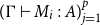 $({\Gamma }\vdash {M_i}:{A})_{j=1}^p$
and the morphisms
 $([\![{M_i}]\!]_{\Gamma }\in \mathcal{L}({{!}} [\![\Gamma ]\!], [\![A]\!]))_{j=1}^p$
are summable. If
 $\sum _{j=1}^pM_j\mathrel {\beta _{\mathsf{cd}}^{\dagger \ast }}\sum _{j=1}^{p'}M'_{j}$
, then the morphisms
 $([\![{M'_j}]\!]_{\Gamma }\in \mathcal{L}({{!}} [\![\Gamma ]\!], [\![A]\!]))_{j=1}^{p'}$
are summable, and we have
 $\sum _{j=1}^p[\![{M_j}]\!]_{\Gamma }=\sum _{j=1}^{p'}[\![{M'_j}]\!]_{\Gamma }$
.
9.4.1 Adequacy and determinism
Now we specialize to the case where
 $\mathcal{L}=\mathbf{Pcoh}$
, see Example 4.2 and 5.2.
If
 ${}\vdash {M}:{A}$
then we know that
 $[\![{M}]\!]_{}\in \mathsf P{ [\![A]\!]}\subseteq (\mathbb{R}_{\geq 0})^{\left |{ [\![A]\!]}\right |}$
. Moreover, a simple inspection of the definition of the semantics shows that actually
 $[\![{M}]\!]_{}\in {\mathbb{N}}^{\left |{ [\![A]\!]}\right |}$
. Of course the situation would be different if the language
 $\mathsf{PCF}_{\mathsf{cd}}$
were extended with a probabilistic choice operator (or more simply, e.g., with a “constant”
 $\mathsf{rand}$
of type
 $\iota$
which has probability
 $1/2$
to reduce to
 $\underline {0}$
and
 $1/2$
to reduce to
 $\underline {1}$
), but this is not the case in the present paper and in Ehrhard (Reference Ehrhard2023a).
If
 $A=\iota$
, this means that
 $[\![{M}]\!]_{}\in {\mathbb{N}}^{\mathbb{N}}$
and that we have
 \begin{align*} \sum _{\nu \in {\mathbb{N}}}{[\![{M}]\!]_{}}_\nu \in [0,1] \end{align*}
so that
 $\forall \nu \in {\mathbb{N}}\ {[\![{M}]\!]_{}}_\nu \in \{0,1\}$
and there is at most one
 $\nu \in {\mathbb{N}}$
such
 ${[\![{M}]\!]_{}}_\nu =1$
. In other words, either
 $[\![{M}]\!]_{}=0$
or
 $[\![{M}]\!]_{}=\mathsf e_{\nu }$
(for a uniquely determined
 $\nu \in {\mathbb{N}}$
).
Theorem 8.4.
Let
 $M$
be a term such that
 ${}\vdash {M}:{\iota }$
and let
 $\nu \in {\mathbb{N}}$
. The two following conditions are equivalent.
-
•
$[\![{M}]\!]_{}=\mathsf e_{\nu }$
-
•
$(\langle {}\rangle ,M,())\mathrel {\beta _{\mathsf{cd}}^{\dagger \ast }}\underline {\nu }$
.

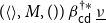
The implication
 $\Leftarrow$
boils down to Corollary 8.2 through the translation
 $\langle {e}\rangle$
from states to terms and Theorem 8.2. The implication
 $\Rightarrow$
is proven using an adaptation of the reducibility method applied to an intersection typing system associated with a relational semantics of
 $\mathsf{PCF}_{\mathsf{cd}}$
which underlies the
 $\mathbf{Pcoh}$
semantics.
So the calculus
 $\mathsf{PCF}_{\mathsf{cd}}$
, and its operational semantics formalized by our Krivine machine, is essentially deterministic in the sense that, starting from a well typed state
 $(\langle {}\rangle ,M,())$
, there is at most one reduction path which leads to a final state
 $(\langle {}\rangle ,M,())$
where
 $\nu \in {\mathbb{N}}$
is uniquely determined by
 $M$
(interpreting the reduction
 $e\mathrel {\rightarrow} e_1+e_2$
as a nondeterministic choice), the other ones leading to
 $0$
. The situation is not completely satisfactory yet since we do not know a priori which transition path is “the good one”.
Another important contribution of Ehrhard (Reference Ehrhard2023a) is a solution of this issue based on a simple and natural idea suggested to the author by Guillaume Geoffroy: make the access word
 $\delta$
of a state
 $(\delta ,N,s)$
writable.
10. Conclusion
We have presented coherent differentiation from a semantical and syntactical point of view, explaining how this new setting combines the ideas of differential LL with determinism and with probabilistic computations.
Even if we consider this as a major improvement wrt. the earlier approaches to differential LL, the precise meaning of the resulting functional calculus is still mysterious. More recently, in a joint work with Aymeric Walch, we have extended this approach to iterated derivatives and to Taylor expansions of terms, still in a deterministic setting (Ehrhard and Walch Reference Ehrhard and Walch2025). These new results might provide the sought programming interpretation of coherent differentiation: it indeed allows one to put, within the language and in a functional way,Footnote 14 strong restrictions on the resource consumption of programs.
Acknowledgments
I would like to thank first my PhD student Aymeric Walch who made many important observations about the first presentation of coherent differentiation in Ehrhard (Reference Ehrhard2023b) of which the present paper has benefited crucially, mainly in Sections 5.2, 5.3 and 6. Many thanks also to the reviewers for their insightful suggestions. This work was partly supported by the ANR project Probabilistic Programming Semantics (PPS) ANR-19-CE48-0014.