


Exploration of the economic aspects of slavery has continued without interruption in the 30 years since the publication of Time on the Cross.1
See the summary in Field-Hendry and Craig, “Relative Efficiency.”
Phillips, American Negro Slavery; Fogel and Engerman, Time on the Cross; Eltis, Economic Growth; and Bergad, “American Slave Markets.”
Genovese, Political Economy; Ashworth, Slavery; and Wright, “Book Review.”
In the Caribbean the idea of the permanent decline of the British slave economy in the last quarter of the eighteenth century, that originated with nineteenth-century abolitionists, and was developed with racist undertones by Lowell Ragatz in the 1920s, continues to receive support.4
Ragatz, Fall; Carrington, Sugar Industry; and Ryden, “Does Decline.”
See Menard, “Slavery”; Burnard, “Grand Mart”; and Irwin, “Wealth Accumulation.”
Two papers by Peter Mancall, Joshua Rosenbloom, and Thomas Weiss examining aspects of output and productivity growth in the Lower U.S. South, are along similar lines. In “Slave Prices and the South Carolina Economy, 1722–1809” (hereafter MRW), our focus here, they combine a slave price series, based largely on probate records, with a price series made up of the main export goods that slaves produced—indigo, cotton, and most importantly rice—to infer trends in average slave productivity. In their other paper, “Agriculture Productivity in the Lower South, 1720–1800,” they marshal an impressive volume of output, input and price data to draw broader implication about productivity growth. It is reassuring that, in certain aspects, the findings of Mancall, Rosenbloom, and Weiss, which are based on a greater variety of data than our estimates for the Caribbean, are similar to our own. They conclude, for example, that the market for slaves in the Americas was open in the long run, and average labor productivity and total factor productivity grew in some periods. Nevertheless, some of their central conclusions hearken back to a traditional view of slavery as inefficient and nonproductive. For example, they find significant differences in the pattern of slave prices between the Caribbean and South Carolina, and large variations even within the mainland colonies. Thus they conclude: “although the long-run supply curve was probably close to perfectly elastic, the short-run supply curve was relatively inelastic.”6
Mancall et al., “Slave Prices,” p. 636.
Mancall et al., “Slave Prices,” p. 636, and “Agricultural Labor Productivity,” pp. 419–20.
The data set, on which we drew to derive our results for the Caribbean, includes slave arrivals in South Carolina and other mainland reception points. During the eighteenth century South Carolina became a major producer of rice, and historians have recently come to focus on the skills that Africans acquired, before they were forced across the Atlantic, and the supposedly strong preferences that South Carolina planters, in particular, had for slaves from rice-growing regions of Africa.8
The hypothesis that South Carolina planters selected slaves from Upper Guinea because of their skills in rice cultivation has become progressively stronger from its first formulation in Wood, Black Majority, through to Judith Carney, Black Rice.
Eltis, Morgan, and Richardson, “African Contribution.”
The MRW sample is for slaves born in the Americas or Africans who had lived in the Americas long enough to enter the probate of their owner. MWR are able to identify the adult male slaves in their sample, but a concern in interpreting their series is the effect of age on slave value. Slaves who entered the probate records would have been older on average but more likely to have developed craft skills than the newly-arrived slaves; as well, one expects that the variation in age would have been much greater. One advantage of the slave trade data is the smaller differences in price due to age. Our series on the sales of newly arrived slaves is much less complete than MRW's, but given the larger sample sizes in those years for which data are available and the greater uniformity, the slave trade data provide a check on the MRW sample and allow us to draw other inferences about the nature of the slave market.
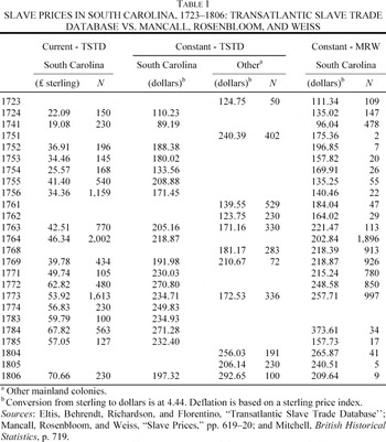
Our series of slave trade prices and the MRW series for years where there is overlap are shown in Table 1. Given the different types of sources, it is perhaps surprising that the slave trade records—records of actual sales, rather than valuations—are so similar to those taken from the probates. Excluding the years 1755, 1783, and 1784, which appear to be outliers even in terms of the MRW sample, the absolute differences average just 10 percent of the slave price. It thus appears that the lower productivity of newly arrived slaves was almost exactly offset by their younger age and, thus, longer productive lifetime. Although the number of years for which data are available is less than one would have liked, there was also little difference between the prices received for newly arrived slaves in South Carolina and the other mainland colonies. This finding is suggestive of a more open market than implied by the MRW comparison of South Carolina and Maryland. In fact, given that newly arrived slaves were more homogeneous, certainly in terms of age, the lower prices of slaves in Maryland after 1760 may indicate a difference in the composition of the slaves for whom prices were obtained.10
Mancall et al., “Slave Prices,” p. 626. A possibly higher proportion of older slaves in the Maryland probates, due to lower mortality and fewer slave imports, may account for the lower slave prices than in South Carolina after 1760.
The merged series is a weighted average of the prices, where the weights are the number of observations in each data set.
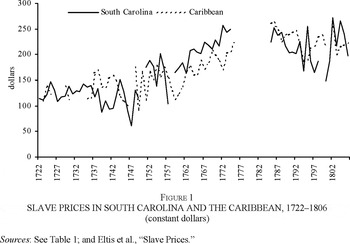
Figure 1 SLAVE PRICES IN SOUTH CAROLINA AND THE CARIBBEAN, 1722–1806 (constant dollars)
Within the Caribbean we found that, with the exception of short periods, the slave trade approximated an open market. Figure 1, which compares our Caribbean slave price series with the price series for South Carolina, indicates that the market for slaves in South Carolina was part of that broader American market. For the period 1722–1775 the average price of slaves in South Carolina was $160 as compared to $152 in the Caribbean. Over the period 1785–1806, South Carolina prices averaged $216 as compared to $227 in the Caribbean. In neither case do we reject the null hypothesis that the mean prices were the same.12
These are constant sterling prices converted to dollars at a rate of 4.44 throughout. The sterling price index is from Mitchell, British Historical Statistics, p. 719.
The t-statistics for sample means are 1.25 (P = 0.218) for the period 1722–1775 and 1.49 (P = 0.152) for the period 1785–1806, not allowing us to reject the null hypothesis of equal means at the 5 percent level. The z statistic for the difference in slopes (based on log-linear regressions) is 2.32 for the period 1722–1775, which is significant at the 5 percent level, and 0.54 for the period 1785–1806, which is not.
Based on a comparison of slave prices with the price of their main output, sugar, we argued in “Slave Prices,” for significant increases in average slave productivity throughout the Caribbean. MRW's approach to productivity was much the same, except in place of the sugar price they used combinations of rice, indigo, and cotton prices depending on the period. It is surprising then, given the similarity of the slave price series for the Caribbean and South Carolina, that MRW find little apparent trend in the ratio of slave prices to the prices of the export goods they produced. The lack of productivity growth is especially puzzling given that during the period 1722 to 1775 slave prices in South Carolina were increasing somewhat faster than in the Caribbean.14
MRW find an upward trend in the ratio of slave prices to output prices to 1775, but argue that this was offset by a decline after the Revolution.
Central to our calculation for the Caribbean was the price of sugar, the main slave output and almost the only cash crop. As noted, MRW use combinations of the price of rice, indigo, and cotton, although given the nature of the calculation it is the price of rice that dominates. For the period 1722 to 1731 the price of rice is from Peter Coclanis's work and after 1731 it is the Charleston wholesale price as reported by Arthur Cole.15
See Coclanis, Shadow, p. 106; and Cole, Wholesale Commodity Prices, p. 154.
The exchange rates for Pennsylvania and South Carolina are from McCusker, Money, pp. 184–86, and 222–24. Rice prices are from Cole, Wholesale Commodity Prices, Statistical Supplement, pp. 7–144. Unweighted monthly averages are used.
Assuming the differential between the farm price and the Charleston price was due entirely to transport costs, a differential of 3 s/cwt implies a cost per (short) ton of $2.41 or 12 cents per ton-mile for a 20-mile haul. Given the change in the price level, this cost is in line with Fogel's estimate of 15 cents per ton-mile for the mid-nineteenth century. See Fogel, Railroads, p. 56. Coclanis (``Rice Prices,” p. 536) notes the distinction between the farm and wholesale price, speculating that the farm price would have been 5 percent to 10 percent lower, a much smaller adjustment than is suggested by the Philadelphia price comparisons.
Another concern is with possible variation in the quality of rice that was brought to the Charleston market. In the Cole data, the quality of rice at both Charleston and Philadelphia is listed as “unspecified.” Coclanis points out that lower quality rice was consumed locally. Some of this rice was “nonmerchantable” and hence would not have entered even the Charleston market; nevertheless, the incentive would have been to export the higher grades and sell more of the lower quality rice in Charleston.18
Coclanis, who puts local rice consumption at one-tenth to one-third of the total crop, points out that this would have included small or broken rice, qualities that would not have been exported. See Coclanis, Shadow, pp. 94, 133.
The quality of rice sold in Philadelphia is also listed as “unspecified,” but given the transport cost from South Carolina it likely would have been of prime quality. The Philadelphia price is adjusted for an assumed transport differential between cities of 3 s/cwt (1774 prices). The transport cost is adjusted using the all-colonial, composite commodity index reported in McCusker, How Much, pp. 52–53.

Figure 2 THE CURRENT PRICE OF RICE AT CHARLESTON AND PHILADELPHIA, AND IN ENGLAND AND HOLLAND, 1722–1806 (1722 = 100)
We follow the MRW approach of using an export price index based on combinations of the prices of rice, indigo, and cotton.20
We assume the same shares as MRW except that in the case of indigo we apply the export data in Gray, History, pp. 1022, 1024, to derive weights rather than assume constant shares of 75 percent for rice and 25 percent for indigo.
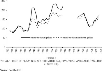
Figure 3 “REAL” PRICE OF SLAVES IN SOUTH CAROLINA, FIVE-YEAR AVERAGE, 1722–1806 (1722 = 100)
As noted by MRW and discussed at some length in Eltis et al., “Slave Prices,” the relation between the ratio of slave to output prices and slave productivity was affected by a number of factors. One of these was the discount rate. If we take the legal interest rate in South Carolina as appropriate, then the decline from 10 percent to 8 percent during the period before the war would imply an increase in productivity of about 75 percent rather than the doubling suggested by the price series alone.21
See Coclanis, Shadow, p.105. This productivity adjustment is based on an expected slave lifetime of 20 years.
Homer and Sylla, History, pp. 276–79.
The “real” slave index that MRW report is based on export prices alone; yet as they carefully document in “Agricultural Labor Productivity,” a substantial part of slave output was consumed domestically. In order to provide a better measure of overall slave productivity rather than productivity based solely on exports, we have derived a slave price index that includes the major nonexported, slave-produced good, corn. We take the wholesale price of Indian corn in Charleston and assign it a weight of 0.5 in the output price index.23
For 1722 to 1731, we use the Philadelphia price of corn adjusted upward by one-third to reflect the later Charleston-Philadelphia differential (see fn. 16). For the Lower South, agricultural exports were likely a smaller share of total agricultural output than 0.5, especially after the Revolution. But if subsistence farm production is excluded a share of 0.5 is perhaps reasonable. See Mancall et al., “Agricultural Labor Productivity,” p. 414; and, for an early-eighteenth-century value, Gray, History, p. 326.
As was true of the Caribbean, increases in slave productivity were achieved despite rapid growth in the slave population. From 1722 to 1775, as MRW report, the slave population increased by a factor of six and over the entire period by a factor of 13.
24Mancall et al., “Slave Prices,” p. 411.

where π is average labor productivity, T is the input of land, L is the input of labor, α is labor's factor share, and superscripts refer to time. An alternate approach, appropriate if one has estimates of land productivity, is to compute total factor productivity as:

where τ is land productivity. Finally one could use a method similar to that used to derive the average productivity estimates by applying the dual of the production function and use output and factor prices. One such specification is:

where P is the price of slaves, R is the rental rate of land, and p is an index of output prices. In Table 2 we report indexes of total factor productivity for the period to the Revolution and for the entire period using each of the measures.

The results point to substantial increases in total factor productivity, with all the increase taking place by the time of the Revolution. Basing the calculation on export goods alone, we estimate using the three different measures that total factor productivity roughly doubled between 1722 and 1770–1774, implying an annual rate of increase over the period of 1.4 percent. According to measure A, which combines labor productivity with the land-labor ratio, total factor productivity increased 103 percent over the period 1722 to 1770–1774, whereas according to measure C, which is based on land prices, it increased by 81 percent. As MRW note and as our series also shows, much of the productivity increase took place after 1740. Important as well is that, despite the dislocation caused by the war, the effect on productivity appears to have been temporary. By 1806 the productivity of South Carolina agriculture was close to the prewar level. Our finding that the productivity of slave agriculture was similar in 1770–1774 and 1802–1806 is not very different from what MRW conclude, but the level that we estimate for each of these periods is much higher.25
Mancall et al., “Agricultural Labor Productivity,” p. 411, put the increase in total factor productivity from 1720 to 1798 at no more than 13 percent.
Measures of productivity based exclusively on prices are less firmly based than those which include data on outputs and inputs. Therefore it is reassuring that the estimates we derive are consistent with descriptions of eighteenth-century rice farming and the advances that were taking place in South Carolina. Irrigation technology, varieties of rice, and task organization improved in the decades after the successful experiments with growing rice in the 1690s.26
See chapter 2 of Max Edelson's forthcoming book, Plantation Enterprise.
Coclanis, Shadow, p. 97.
The evidence on South Carolina points to large advances in productivity associated mainly with rice farming, but for the major questions about slavery and its role in the development of the Americas, we need to observe the larger playing field. The South Carolina slave price data should be seen as just part of an assessment of trends in the plantation economy of the Americas as a whole. In 1790 South Carolina contained less than 3 percent of the Americas' slave population; and it produced rice and indigo, whereas the overwhelming reason slaves traveled across the Atlantic was sugar. Moreover, indigo, which accounted for as much as one-third of the region's export revenues, was heavily dependent on British bounties, and this revenue source largely disappeared after independence as the bounties were removed. But, despite the sudden variation in export crops, productivity remained high after the war; and over the entire period the increase in productivity paralleled that in the Caribbean. In the past two decades strong evidence of nineteenth-century technology gains has emerged for the export sectors of the U.S. South and other parts of the Americas. It now appears that such a pattern was well established before 1800.
The authors are grateful to Joshua Rosenbloom, Peter Mancall, and Tom Weiss for providing us with their data files.


