2. Modelling equations

In order to investigate the nonlinear dynamic evolution of NDTMs, a standard reduced MHD model in a cylindrical coordinate system $(r,\theta ,z)$ is employed in this work (Strauss Reference Strauss1976; Hazeltine, Kotschenreuther & Morrison Reference Hazeltine, Kotschenreuther and Morrison1985; Sato & Wakatani Reference Sato and Wakatani2005). The normalised governing equations are expressed as follows:

(2.1) \begin{equation}\frac{\partial \psi }{\partial t}=\left[\psi ,\phi \right]-\partial _{z}\phi -{S}_{A}^{-1}(j-j_{b})+E_{z0},\end{equation}

(2.2) \begin{equation}\frac{\partial u}{\partial t}=\left[u,\phi \right]+\left[j,\psi \right]+\partial _{z}j+R^{-1}{\boldsymbol{\nabla} }_{\bot }^{2}u,\end{equation}

(2.3) \begin{equation}\frac{\partial p}{\partial t}=\left[p,\phi \right]+\chi _{\parallel }{\boldsymbol{\nabla} }_{\parallel }^{2}p+\chi _{\bot }{\boldsymbol{\nabla} }_{\bot }^{2}p+S_{0}.\end{equation}

Here, $\psi$ , $\phi$ and $p$ represent the poloidal magnetic flux, the stream function and the plasma pressure, respectively. The variables $j=-{\boldsymbol{\nabla} }_{\bot }^{2}\psi$ and $u={\boldsymbol{\nabla} }_{\bot }^{2}\phi$ in the equations denote the plasma current density and the vorticity along the axial direction, respectively. Under the reduced MHD approximation, assuming that the poloidal rotation is mainly provided by the $E\times B$ drift, the plasma velocity field can be expressed as $\boldsymbol{v}=-\boldsymbol{\nabla }\phi \times \hat{z}$ (where $\phi$ is equivalent to the electrostatic potential) (Zhang & Ma Reference Zhang and Ma2009; Wang & Wang Reference Wang and Wang2015). The nonlinear Poisson bracket included in (2.1)–(2.3) is defined as $[f,g]=\hat{z}\boldsymbol{\cdot }(\boldsymbol{\nabla }f\times \boldsymbol{\nabla }g)$ . The gradient operator parallel to the magnetic field is defined as $\boldsymbol{\nabla} _{\parallel }S=\partial S/\partial z+[S,\psi ]$ .

A standard normalisation scheme is adopted in this model. For the spatial coordinates, the radial distance $r$ is normalised by the plasma minor radius $a$ . The time $t$ and the velocity field $v$ are normalised in units of the Alfvén time $\tau _{A}=a\sqrt{\mu _{0}\rho }/B_{0}$ and the Alfvén velocity $v_{A}=B_{0}/\sqrt{\mu _{0}\rho }$ , respectively. Accordingly, the poloidal magnetic flux $\psi$ , the stream function $\phi$ and the plasma pressure $p$ are normalised by $aB_{0}$ , $aB_{0}v_{A}$ and the initial pressure at the magnetic axis, respectively. The expression $\beta _{e}=2\mu _{0}n_{0}T_{e}/{B}_{0}^{2}$ is used to characterise the ratio of the thermal pressure to the magnetic pressure. The dimensionless dissipation coefficients are characterised by the magnetic Reynolds number $S_{A}=\tau _{\eta }/\tau _{A}$ , the kinematic Reynolds number $R=\tau _{\nu }/\tau _{A}$ and the heat transport coefficients $\chi _{\parallel }$ and $\chi _{\bot }$ . Here, $\tau _{\eta }=a^{2}\mu _{0}/\hat{\eta }$ and $\tau _{\nu }=a^{2}/\hat{\mu }$ denote the resistive and viscous diffusion times, respectively. The heat transport coefficients $\chi _{\parallel }$ and $\chi _{\bot }$ are both normalised to $a^{2}/\tau _{A}$ . The term $j_{b}$ in (2.1) is the bootstrap current density driven by the radial pressure gradient, and its magnitude is determined by the bootstrap current fraction defined as $f_{b}=\int\! j_{b0}r{\rm d}r/\int\! j_{z0}r{\rm d}r$ . Furthermore, the source terms $E_{z0}={S}_{A}^{-1}(j_{0}-j_{b0})$ and $S_{0}=-\chi _{\bot }{\boldsymbol{\nabla} }_{\bot }^{2}p_{0}$ in (2.1) and (2.3) are chosen to balance the diffusions of the initial equilibrium profiles of the ohmic current ( $j_{\mathrm{ohm}}=j_{0}-j_{b0}$ ) and pressure, respectively.

Any physical variable $f(r,{\unicode[Arial]{x03B8}} ,z,t)$ in the system can be decomposed into an initial equilibrium term $f_{0}(r)$ that is independent of time and a perturbation term $\tilde{f}(r,{\unicode[Arial]{x03B8}} ,z,t)$ that evolves with time. By applying periodic boundary conditions in the poloidal and axial directions, the perturbed fields can be expanded via Fourier transform as

(2.4) \begin{equation}\tilde{f}\left(r,\theta ,z,t\right)=\frac{1}{2}\sum\nolimits_{m,n}\tilde{f}_{m,n}\left(r,t\right)\exp \left(im\theta -inz/R_{0}\right)+c.c.\end{equation}

where $m$ and $n$ are the poloidal and toroidal mode numbers, respectively, and $R_{0}$ is the major radius of the tokamak. To analyse the magnetic reconnection process, the equilibrium helical flux associated with a given $m/n$ perturbation is defined as

(2.5) \begin{equation}{\psi }_{m/n}^{*}(r)={\int }_{0}^{r}r'\left[\frac{1}{q(r')}-\frac{n}{m}\right]{\rm d}r'.\end{equation}

In cylindrical geometry, ${\psi }_{m/n}^{*}$ represents the equilibrium magnetic flux in the frame moving with the helical pitch of the $m/n$ perturbation. Its radial derivative satisfies

(2.6) \begin{equation}\frac{{\rm d}{\psi }_{m/n}^{\mathrm{*}}}{{\rm d}r}=r\left[\frac{1}{q(r)}-\frac{n}{m}\right]\!,\end{equation}

so the stationary points of ${\psi }_{m/n}^{*}$ correspond to the resonant surfaces $q(r) = m/n$ . When the corresponding perturbation is included, the contours of the total helical flux are used to identify the O points, X points and separatrix structures of magnetic islands (Yu Reference Yu1997).

Figure 1.

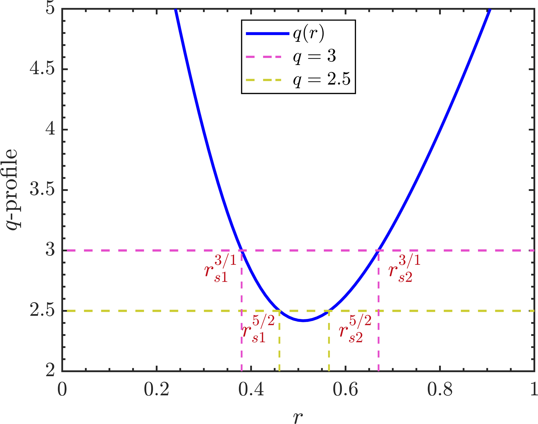
The safety factor $q$ -profile with ${r}_{s1}^{3/1},{r}_{s2}^{3/1}$ and ${r}_{s1}^{5/2},{r}_{s2}^{5/2}$ indicating the inner and outer rational surfaces of the $m/n=3/1$ and $m/n=5/2$ modes, respectively.

Given the initial profiles, the three-dimensional initial-value code MHD@Dalian is utilised to solve equations in this work. For the spatial discretisation, the finite difference method is adopted in the radial direction, and the pseudospectral method is employed in the poloidal and axial directions; the time advancement employs a two-step predictor–corrector method. An ideally conducting wall condition is assumed at the radial boundary, i.e. satisfying $\tilde{\psi }_{m,n}=\tilde{\phi }_{m,n}=\tilde{u}_{m,n}=\tilde{p}_{m,n}=0$ at $r=1$ . The MH nonlinear simulations are performed in this paper, and the ranges of poloidal and toroidal mode numbers included in the calculations are $0 \leq m \leq 24$ and $0 \leq n \leq 8$ , respectively. As shown in figure 1, the initial safety factor $q$ profile is set with typical RMS characteristics, where two pairs of rational surfaces with different helicities (corresponding to $h=3/1$ and $h=5/2$ , respectively) coexist in the radial direction. The computational domain is discretised with $N_{r}=1500$ radial grid points. Other fixed parameters are ${S}_{A}^{-1}=5\times 10^{-6}$ , $R^{-1}=1\times 10^{-6}$ , the inverse aspect ratio $\varepsilon _{a}=a/R_{0}=0.25$ , $\chi _{\parallel }=10$ and $\chi _{\bot }=10^{-6}$ . The present numerical set-up follows the parameter range commonly used in previous reduced MHD simulations of long-time DTM/NDTM evolution in RMS plasmas. Similar values of ${S}_{A}^{-1}$ , $R^{-1}$ , $\chi _{\parallel }$ and $\chi _{\bot }$ have been adopted in earlier studies of intermittent DTM bursts, and the MHD@Dalian code has been benchmarked and applied to nonlinear NDTM dynamics in RMS configurations. In these previous applications, the cylindrical reduced MHD formulation has provided a useful framework for isolating the essential nonlinear processes of tearing mode evolution, including rational surface reconnection, mode coupling, bootstrap current effects and $q$ -profile recovery. Following this framework, the adopted dissipation and transport coefficients are kept fixed in all SH/MH and $f_{b}$ -scan cases, so that the relative effects of MH coupling and bootstrap current fraction are compared under the same numerical and dissipative conditions. The radial resolution $N_{r}=1500$ and the spectral range $0\leq m\leq 24, 0\leq n\leq 8$ are sufficient for resolving the dominant $3/1$ mode, the subdominant $5/2$ mode and the main coupled harmonics discussed in the following (Wang et al. Reference Wang, Liu and Wei2022a ; Ren et al. Reference Ren, Wei, Li and Wang2024). Although toroidal curvature, Shafranov shift and neoclassical viscosity beyond the bootstrap current contribution are not explicitly retained in this cylindrical formulation, they are expected to play an important role in determining the quantitative behaviour of realistic tokamak plasmas (Hahm Reference Hahm1988; Nishimura, Callen & Hegna Reference Nishimura, Callen and Hegna1998; Lütjens et al. Reference Lütjens, Luciani and Garbet2001). These effects may modify the linear growth rates, nonlinear saturation levels and transition values, while the qualitative nonlinear trends discussed in the following are governed primarily by magnetic topology, modal energy redistribution and current profile evolution. Direct quantitative comparisons with JET, EAST and HL-2A experiments or toroidal simulations are beyond the current scope. However, this framework is fully sufficient for isolating the underlying nonlinear mechanisms. Benchmarking against experimental data and cross-code verification will be systematically pursued as the primary focus of future research.

3. Numerical results

In this section, the intermittent bursts and nonlinear coupling phenomena of NDTMs in the RMS configuration are systematically investigated via both MH and SH simulations based on the safety factor profile introduced in § 2.

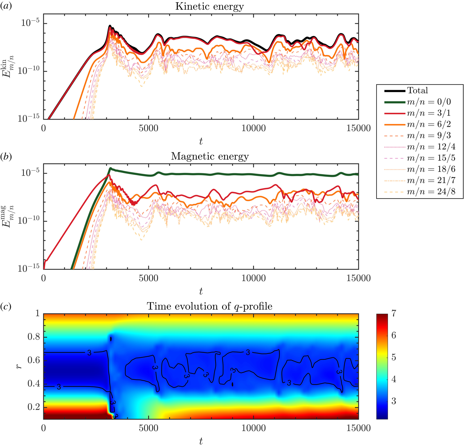
The SH simulation is first performed with an $m/n=3/1$ mode initial perturbation, neglecting the bootstrap current ( $f_{b}=0$ ). The time evolutions of the kinetic and magnetic energy of the $3/1$ mode and its higher harmonics, as well as the safety factor profile, are shown in figure 2(a–c). After the first explosive burst at $t=0.3\times 10^{4}$ , the system enters the nonlinear phase. The intermittent burst period starting at $t=0.5\times 10^{4}$ is selected as the first intermittent burst for analysis. During each burst, the kinetic and magnetic energy increase rapidly and then decay after reaching their peak values. Meanwhile, the safety factor between the two $3/1$ rational surfaces is lifted to greater than 3, causing the resonant surfaces to disappear temporarily. As the ohmic current recovers, the $q$ profile gradually returns to the initial unstable state, and the next intermittent burst is then triggered.

Figure 2.

(a) Time evolutions of kinetic energy ${E}_{m/n}^{kin}$ and (b) time evolutions of the magnetic energy ${E}_{m/n}^{mag}$ for different harmonics and (c) dynamic change of the safety factor profile in the SH simulation for $f_{b}=0$ .

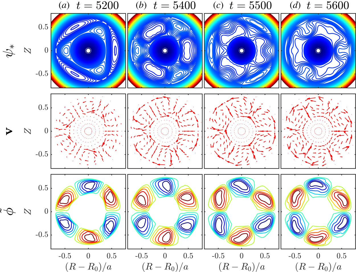
Figure 3 displays the helical magnetic flux contours, the velocity vector field and the stream function contours for the SH simulation with $f_{b}=0$ . At $t=0.52\times 10^{4}$ , magnetic islands are formed on the two rational surfaces. At $t=0.54\times 10^{4}$ , the magnetic islands grow continuously; the outer magnetic islands move inward while the inner ones move outward. Consequently, the open magnetic field lines between the inner and outer islands reconnect. The plasma velocity is directed from the X points towards the O points, and the velocity field reaches its maximum at the X points of the magnetic islands where the stream function contours are most concentrated. At $t=0.55\times 10^{4}$ , the radial positions of the inner and outer islands are exchanged, and a magnetic separatrix reappears between the islands. Finally, at $t=0.56\times 10^{4}$ , the magnetic islands are almost completely consumed, and the open magnetic field lines reappear, indicating that the intermittent burst is approaching its end.

Figure 3.

Typical helical magnetic flux contours, $\psi _{*}$ (i); velocity vector fields $\boldsymbol{v}$ (ii); and stream function contours, $\tilde{\phi }$ (iii) at different time slices during the intermittent bursts in the SH simulation for $f_{b}=0$ .

Figure 3. Long description

The image contains three rows of contour plots and vector fields, each row representing different aspects of the plasma simulation at four different time slices. Panel A shows the helical magnetic flux contours at times t = 5200, t = 5400, t = 5500, and t = 5600. The contours are color-coded, with blue indicating lower values and red indicating higher values. The contours form intricate patterns that evolve over time. Panel B displays the velocity vector fields at the same time slices. The vectors are shown in red and indicate the direction and magnitude of the velocity field. The vectors form symmetrical patterns that change over time. Panel C presents the stream function contours at the same time slices. The contours are color-coded, with blue indicating lower values and red indicating higher values. The contours form circular patterns that evolve over time. The horizontal axis is labeled (R - R0)/a and ranges from -0.5 to 0.5. The vertical axis is labeled z and ranges from -0.5 to 0.5. The contours and vectors show the dynamic behavior of the plasma during the intermittent bursts in the simulation.

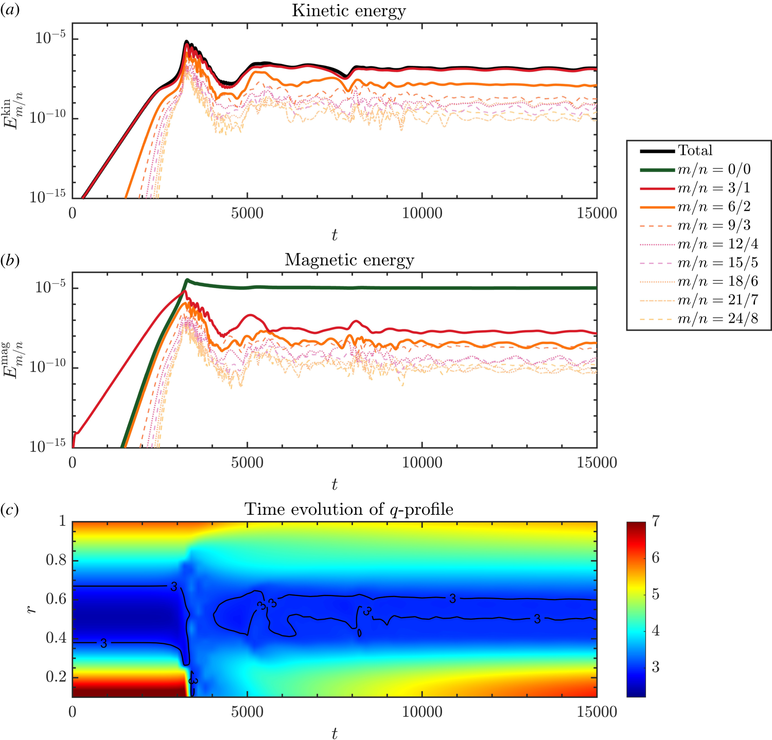
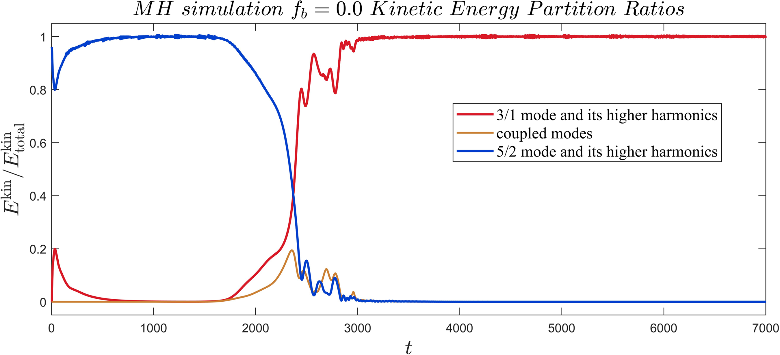
In the MH simulation without bootstrap current ( $f_{b}=0$ ), initial perturbations of both the $3/1$ and $5/2$ modes are introduced. The coexistence of different helicities alters the nonlinear evolution of the system. The time evolutions of the kinetic and magnetic energies of the $3/1$ mode, the $5/2$ mode and the high-order harmonics, together with the safety factor profile, are shown in figure 4(a–c). To further illustrate the redistribution of perturbation energy among different helicities, figure 5 presents the kinetic energy partition ratios, where the total kinetic energy is divided into three parts: the $3/1$ mode and its higher harmonics; the $5/2$ mode and its higher harmonics; and the coupled modes generated by nonlinear interaction. In the early phase of the evolution, since the distance between the two rational surfaces of the $5/2$ mode is smaller, its linear growth rate is higher than that of the $3/1$ mode. Consequently, the $5/2$ mode reaches saturation first at $t=0.2\times 10^{4}$ . This is also reflected in figure 5, where the $5/2$ mode and its higher harmonics occupy the dominant part of the non-axisymmetric kinetic energy during the early nonlinear stage. At this time, the $3/1$ mode is still growing. When the $5/2$ mode saturates, the growth rate of the $3/1$ mode exhibits a transient increase, which is associated with nonlinear coupling induced by the saturated $5/2$ mode. As the system approaches the first burst, the energy fraction of the $3/1$ mode and its higher harmonics rises rapidly, while the coupled modes also show a finite transient contribution. This indicates that, in the MH case, the perturbation energy is not confined to a single $3/1$ harmonic chain, but is distributed through additional nonlinear energy channels associated with the $5/2$ mode and the coupled modes. After this transient coupling stage, the $3/1$ mode enters the Rutherford regime and subsequently undergoes the first explosive burst. Meanwhile, the modes generated by the coupling between the $5/2$ and $3/1$ modes, such as the $8/3$ mode, also reach saturation. As shown in figure 4(c), the burst of the $3/1$ mode causes the $q$ profile between the resonant surfaces to rise rapidly and become flattened to greater than $q=3$ . This modification causes the resonant surfaces satisfying $q=2.5$ to disappear within the plasma region. Therefore, although residual perturbation energy remains in the system, the $5/2$ mode cannot be sustained without its resonance condition, and its amplitude gradually decreases until it is suppressed. The system finally returns to an intermittent bursting phase dominated by the $3/1$ mode and its higher harmonics, exhibiting an evolution behaviour similar to that in the SH case.

Figure 4.

(a) Time evolutions of kinetic energy ${E}_{m/n}^{kin}$ and (b) time evolutions of the magnetic energy ${E}_{m/n}^{mag}$ for different harmonics and (c) dynamic change of the safety factor profile in the MH simulation for $f_{b}=0$ .

Figure 5.

Kinetic energy partition ratios in the MH simulation with $f_{b}=0$ . The total kinetic energy is divided into three parts: the $3/1$ mode and its higher harmonics; the $5/2$ mode and its higher harmonics; the coupled modes generated by nonlinear interaction.

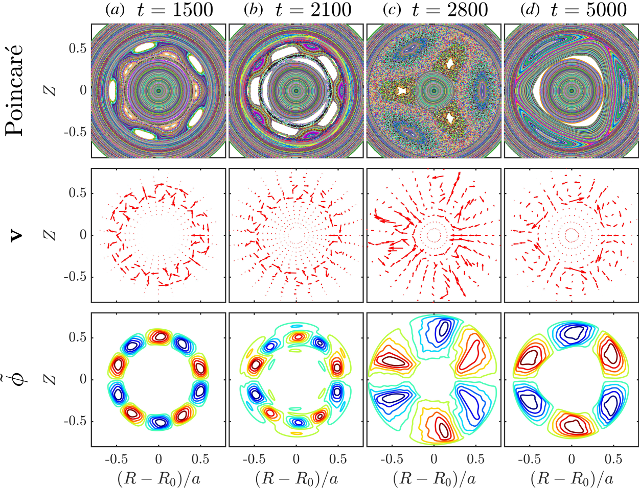
Figure 6 presents the Poincaré plots, velocity vector fields and stream function contours for the MH simulation with $f_{b}=0$ . After entering the nonlinear phase, since the distance between the rational surfaces of the $5/2$ mode is small, it grows faster than the $3/1$ mode. At $t=1500$ , the $5/2$ mode has saturated and exhibits an exchange of inner and outer islands, accompanied by an oscillation in kinetic and magnetic energy. At $t=2100$ , as the $3/1$ mode continues to grow and its magnetic islands become sufficiently large, perturbations from both modes can be observed in the stream function and velocity vector fields. Simultaneously, the spatial overlap of the $3/1$ and $5/2$ modes, as well as the high-order magnetic islands (e.g. $8/3$ mode) generated by their coupling, induces strong magnetic stochasticity between the resonant surfaces of the $3/1$ and $5/2$ modes. At $t=2800$ , the $3/1$ mode grows to saturation and undergoes the first explosive burst. The energy of the modes generated by the coupling of the $3/1$ and $5/2$ modes also reach its maximum, and the range influenced by magnetic stochasticity becomes maximal. At $t=5000$ , due to the suppression of other modes by the $3/1$ mode, only the intermittent oscillation dominated by the $3/1$ mode exists, as evidenced by the Poincaré plots, the velocity vector fields and the stream function contours where only the magnetic islands and perturbations of the $3/1$ mode remain while the magnetic stochasticity and magnetic islands of other modes have disappeared.

Figure 6.

Poincaré plots of magnetic field lines in a poloidal cross-section (i); velocity vector fields, $\boldsymbol{v}$ (ii), and stream function contours, $\tilde{\phi }$ (iii) at different time slices in the MH simulation for $f_{b}=0$ .

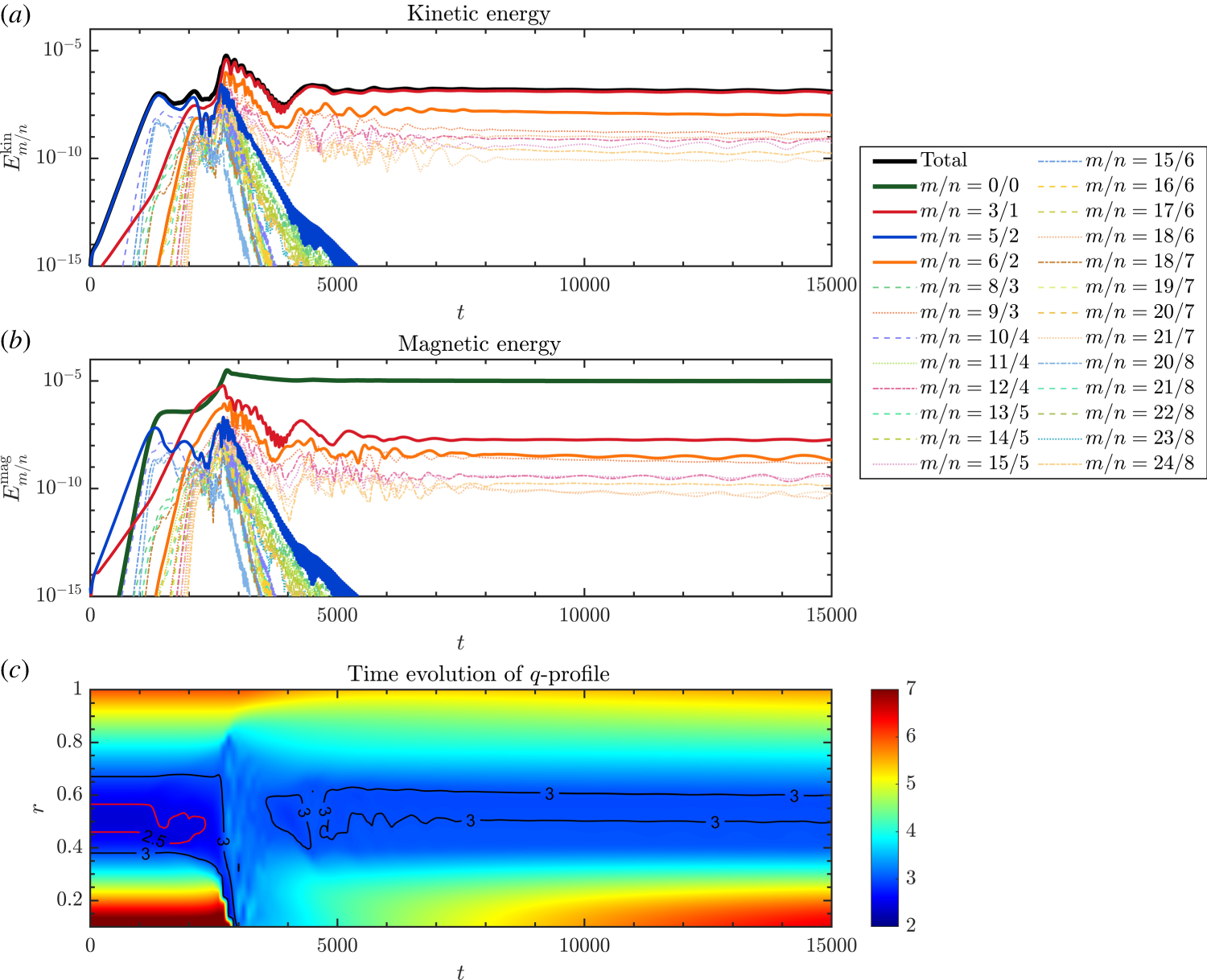
With increasing $f_{b}$ , the results of kinetic energy, magnetic energy and safety factor profiles for SH and MH simulations with $f_{b}=0.2$ are shown in figures 7(a–c) and 8(a–c), respectively. During the intermittent oscillation process after the first explosive burst, it is observed that the amplitudes of kinetic and magnetic energy and the distance between the inner and outer resonant surfaces are significantly reduced compared with those in the $f_{b}=0$ case. This is attributed to the fact that, under the condition of maintaining the total current constant, as $f_{b}$ increases, the proportion of the ohmic current in the source term $E_{z0}$ , which is responsible for restoring the unstable $q$ -profile, decreases. Therefore, the capability of the system to restore the magnetic configuration is weakened, the distance between rational surfaces cannot fully return to the initial equilibrium position and the intensity of subsequent bursts is reduced.

Figure 7.

(a) Time evolutions of kinetic energy ${E}_{m/n}^{kin}$ and (b) time evolutions of the magnetic energy ${E}_{m/n}^{mag}$ for different harmonics and (c) dynamic change of the safety factor profile in the SH simulation for $f_{b}=0.2$ .

Figure 7. Long description

The image contains three graphs. Panel A: A line graph shows the time evolution of kinetic energy for different harmonics. The x-axis represents time (t) in arbitrary units, and the y-axis represents the kinetic energy (E_kin) in arbitrary units. The graph includes multiple lines, each representing a different harmonic (m/n) ratio, with a legend indicating the specific ratios. The total kinetic energy is also shown. Panel B: Another line graph displays the time evolution of magnetic energy for different harmonics. The x-axis represents time (t) in arbitrary units, and the y-axis represents the magnetic energy (E_mag) in arbitrary units. Similar to Panel A, multiple lines represent different harmonics, with a legend indicating the specific ratios. The total magnetic energy is also shown. Panel C: A heatmap illustrates the dynamic change of the safety factor profile over time. The x-axis represents time (t) in arbitrary units, and the y-axis represents the radial position (r) in arbitrary units. The color scale on the right indicates the safety factor values, with contours marking specific values. The heatmap shows the evolution of the safety factor profile, with annotations indicating specific values at different times.

Figure 8.

(a) Time evolutions of kinetic energy ${E}_{m/n}^{kin}$ and (b) time evolutions of the magnetic energy ${E}_{m/n}^{mag}$ for different harmonics and (c) dynamic change of the safety factor profile in the MH simulation for $f_{b}=0.2$ .

Furthermore, with increasing $f_{b}$ , the MH evolution appears to exhibit an additional coupling related acceleration effect. As shown by the kinetic energy evolution in the MH simulation with $f_{b}=0.2$ (figure 8 a), when the $5/2$ mode reaches saturation, the growth rate of the $3/1$ mode increases and remains at an elevated level, so that the $3/1$ mode directly enters the Rutherford regime and undergoes the first explosive burst. This behaviour is distinct from the $f_{b}=0$ case (figure 4 a), where the saturation of the $5/2$ mode causes only a momentary increase in the growth rate of the still unsaturated $3/1$ mode, after which the growth rate returns to its previous level before the $3/1$ mode continues its evolution towards the Rutherford regime. This difference suggests that, in the presence of bootstrap current, nonlinear mode coupling can provide an additional drive for the dominant mode and thereby accelerate its entry into the first burst.

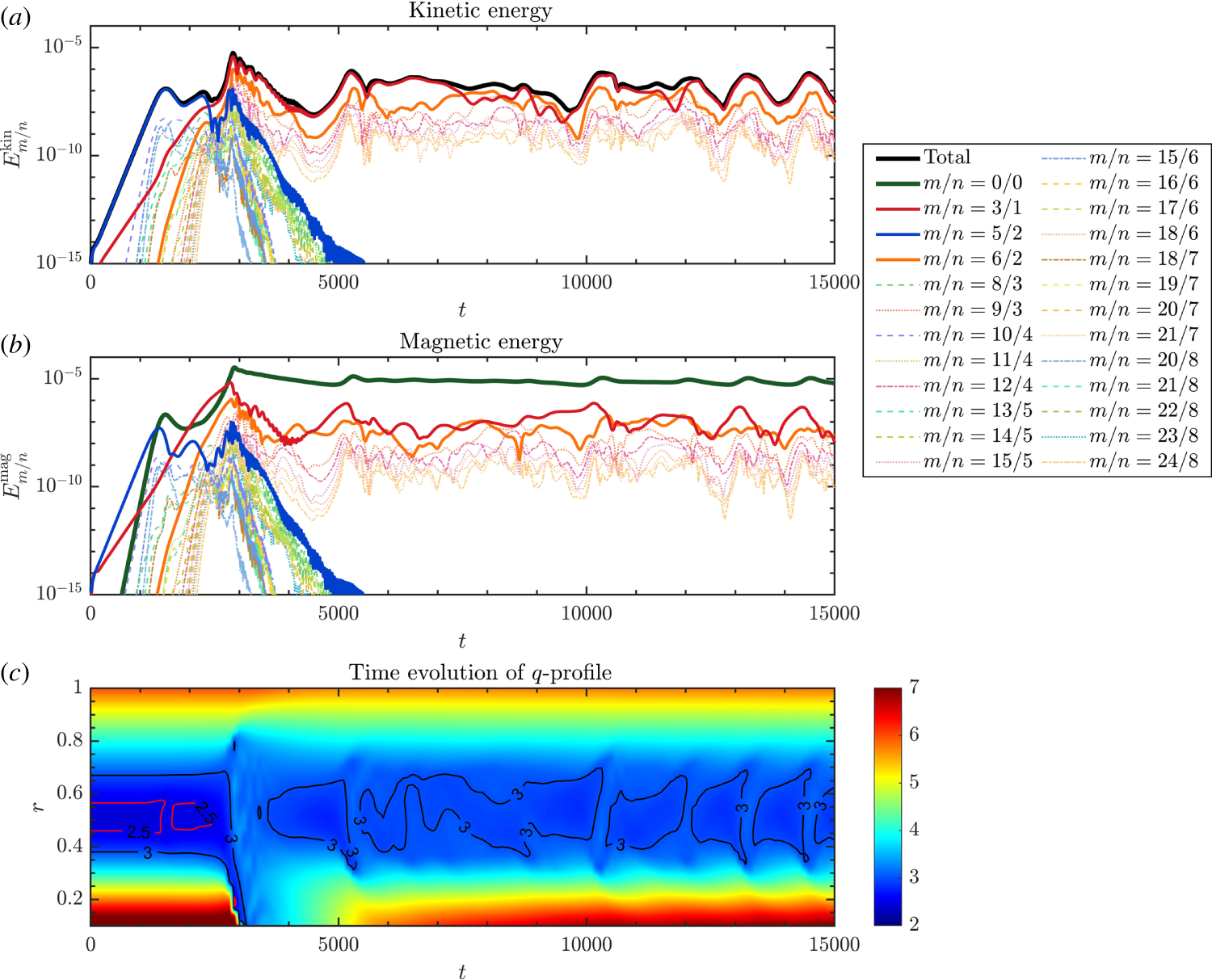
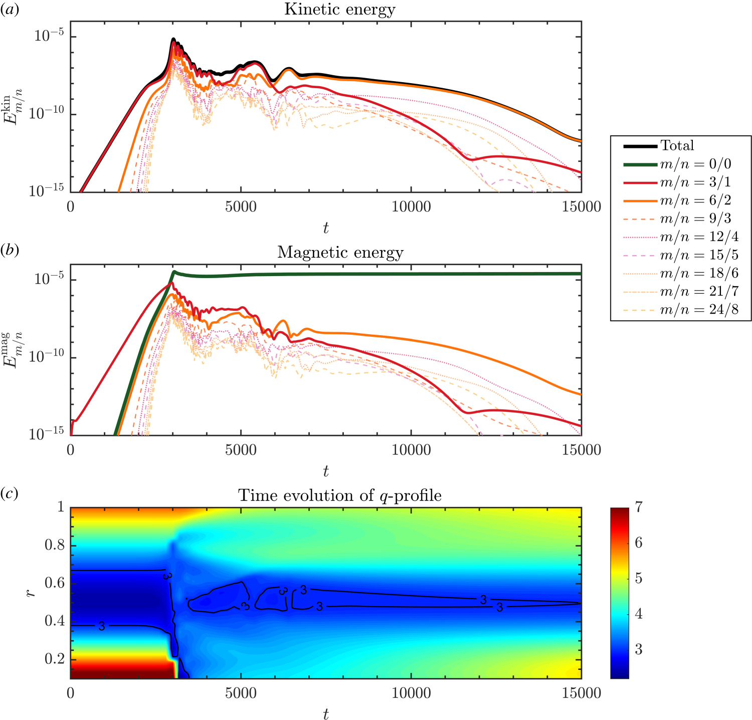
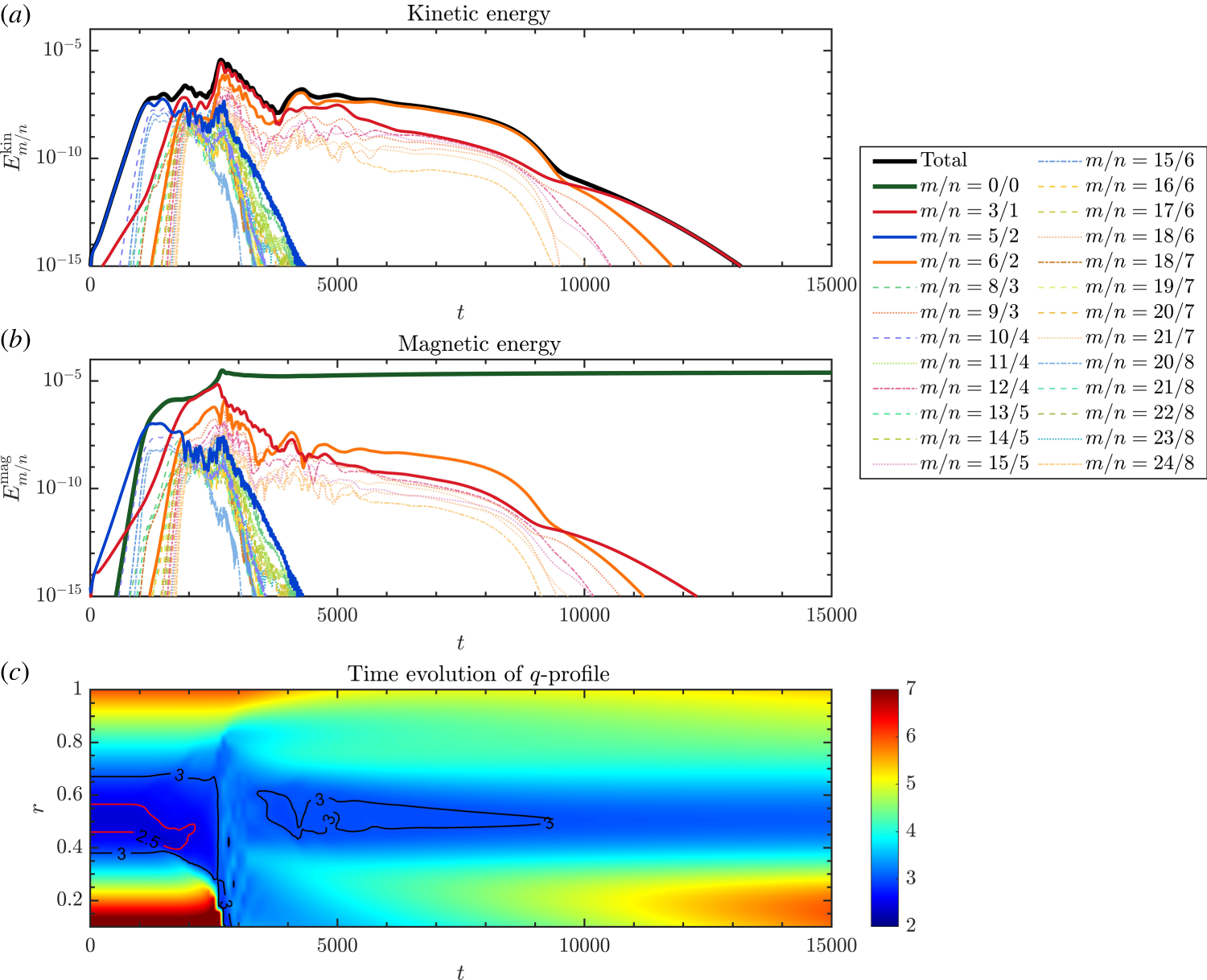
When the bootstrap current fraction is further increased to $f_{b}=0.4$ , the intermittent bursting phenomenon disappears, as shown in the SH simulation (figure 9 a–c) and the MH simulation (figure 10 a–c). Due to the reduced ohmic current contribution in the source term, the flattening of the $q$ profile induced by reconnection cannot be effectively reversed. Simulation results indicate that after the first explosive burst, the safety factor is gradually raised to greater than $3$ , and the unstable condition for the DTM is no longer satisfied. The kinetic and magnetic energy of the $3/1$ mode, $5/2$ mode and high-order harmonics exhibit a monotonic decreasing trend, and the system tends towards a stable state.

Figure 9.

(a) Time evolutions of kinetic energy ${E}_{m/n}^{kin}$ and (b) time evolutions of the magnetic energy ${E}_{m/n}^{mag}$ for different harmonics and (c) dynamic change of the safety factor profile in the SH simulation for $f_{b}=0.4$ .

Figure 9. Long description

The image contains three panels showing different aspects of a simulation. Panel A: A line graph displays the time evolution of kinetic energy for different harmonics. The x-axis represents time (t) in arbitrary units, and the y-axis represents the kinetic energy (E_kin) in arbitrary units. The graph includes multiple lines, each representing a different harmonic (m/n), with a legend indicating the specific harmonics. The total kinetic energy is also shown. Panel B: Another line graph shows the time evolution of magnetic energy for the same harmonics. The x-axis is time (t) in arbitrary units, and the y-axis is magnetic energy (E_mag) in arbitrary units. Similar to Panel A, multiple lines represent different harmonics, with a legend for reference. The total magnetic energy is also included. Panel C: A heatmap illustrates the dynamic change of the safety factor profile over time. The x-axis represents time (t) in arbitrary units, and the y-axis represents the radial position (r) in arbitrary units. The color scale on the right indicates the safety factor values, with contours marking specific values. The heatmap shows the evolution of the safety factor profile, with annotations indicating specific values at different times.

Figure 10.

(a) Time evolutions of kinetic energy ${E}_{m/n}^{kin}$ and (b) time evolutions of the magnetic energy ${E}_{m/n}^{mag}$ for different harmonics and (c) dynamic change of the safety factor profile in the MH simulation for $f_{b}=0$ .4.

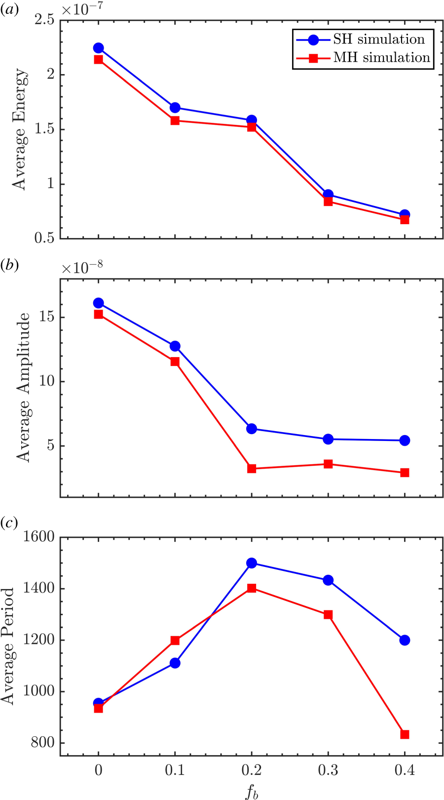
Figure 11(a–c) presents a comparison of the average energy, average amplitude and average period of the intermittent bursts between the SH and MH simulations. From figures 11(a) and 11(b), it can be seen that the average energy and burst amplitude of the dominant mode ( $3/1$ mode) in the MH simulation are lower than those in the SH simulation. This can be attributed to the redistribution of perturbation energy in the MH case. Starting from the same initial state, part of the energy is distributed to the 5/2 mode and the higher-order harmonics generated by nonlinear coupling in the early stage of the evolution, thereby reducing the energy available to the dominant $3/1$ mode and resulting in lower average burst energy and amplitude than in the SH case.

Figure 11.

Comparisons of (a) the average energy, (b) the average amplitude and (c) the average period of intermittent bursts in the SH and MH simulations with different bootstrap current fractions. The statistical interval is selected from the first energy minimum after the initial explosive burst to the last energy minimum before $t=15\,000$ . Within this interval, the average energy is obtained by time-averaging the dominant mode energy; the average amplitude is calculated as the mean peak to valley energy variation of each burst cycle; and the average period is evaluated from the mean time interval between adjacent energy peaks.

Figure 11. Long description

Three line graphs depict comparisons of average energy, amplitude, and period of intermittent bursts in SH and MH simulations with different bootstrap current fractions. Panel A: The line graph shows average energy on the vertical axis, ranging from 0.5 to 2.5 times 10^-7, and bootstrap current fraction (f_b) on the horizontal axis, ranging from 0 to 0.4. Two data series are plotted: SH simulation in blue circles and MH simulation in red squares. Both series show a decreasing trend in average energy as the bootstrap current fraction increases. Panel B: The line graph shows average amplitude on the vertical axis, ranging from 0 to 15 times 10^-8, and bootstrap current fraction (f_b) on the horizontal axis, ranging from 0 to 0.4. Two data series are plotted: SH simulation in blue circles and MH simulation in red squares. Both series show a decreasing trend in average amplitude as the bootstrap current fraction increases, with the SH simulation showing a more pronounced decrease. Panel C: The line graph shows average period on the vertical axis, ranging from 800 to 1600, and bootstrap current fraction (f_b) on the horizontal axis, ranging from 0 to 0.4. Two data series are plotted: SH simulation in blue circles and MH simulation in red squares. Both series show an initial increase in average period, peaking around a bootstrap current fraction of 0.2, followed by a decrease.

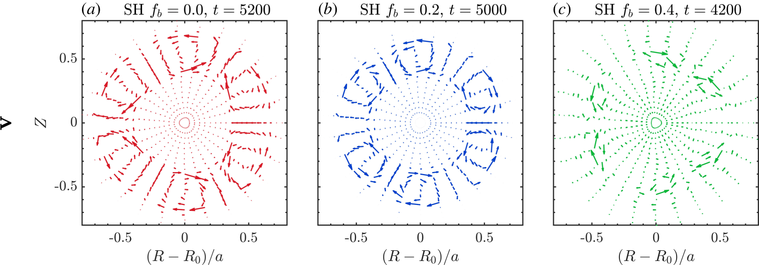
The bootstrap current fraction has an important impact on the energy intensity of the intermittent bursts. As the bootstrap current fraction increases while the total current is kept constant, the ohmic current contribution to restoring the magnetic configuration decreases, so that the $q$ -profile becomes less capable of returning to its initial unstable state between two bursts. Consequently, the distance between the two rational surfaces decreases, and so does the spatial extent of the corresponding perturbation velocity fields, as shown in figure 12. As a result, the system can accumulate less energy between intermittent bursts, and the energy released during each reconnection event is also reduced, leading to a decreasing trend in the average energy and the average amplitude with increasing $f_{b}$ . Meanwhile, because the recovery towards the next unstable state becomes slower, the time required to trigger the subsequent burst is prolonged, and thus the burst period increases with the bootstrap current fraction.

Figure 12.

Velocity vector fields ( $\boldsymbol{v}$ ) during the intermittent oscillation process in the SH simulation with different bootstrap current fractions: (a) $f_{b}=0$ ; (b) $f_{b}=0.2$ ; (c) $f_{b}=0.4$ .

Furthermore, in the present equilibrium, when the bootstrap current fraction increases to approximately $f_{b}=0.2$ , the intermittent bursts of the dominant mode exhibit a different nonlinear pattern: the burst amplitude tends to saturate, while the burst period gradually decreases. This transition is closely related to the competition between reconnection induced $q$ -profile relaxation and ohmic current driven profile restoration. As $f_{b}$ increases while the total current is kept fixed, the ohmic current contribution in $E_{z0}={S}_{A}^{-1}(j_{0}-j_{b0})$ decreases, and the recovery of the $q$ profile becomes increasingly limited. Under this condition, the system still remains in an intermittent bursting state, but the bursts evolve into a smaller amplitude form on a lower energy basis. As a result, the energy accumulated and released in each cycle remains constrained, leading to the saturation of the burst amplitude. Meanwhile, because the excursion of each intermittent burst becomes smaller, the dominant mode can reach the next reconnection condition over a shorter interval, and the burst period therefore decreases gradually.

Further comparison between the SH and MH simulation results reveals that under higher bootstrap current conditions, both the average amplitude and the average period of the dominant mode in the MH system are significantly smaller than those in the SH case. For example, in the present equilibrium, at $f_{b}=0.4$ , the average amplitude is reduced by approximately 46.18 %, and the burst period is shortened by approximately 30.56 %. At this bootstrap current fraction, the ohmic restoration is further weakened, so that the system can hardly re-establish a strongly unstable double tearing configuration after the first crash. This difference also reflects the evolutionary characteristics of the MH system. In the early phase of the MH evolution, part of the perturbation energy is distributed into the $5/2$ mode and its higher harmonics as well as the coupled modes, so that the burst intensity of the dominant mode is lower than that in the SH case. After entering the nonlinear phase, the coupled modes in the MH system are significantly suppressed, and the system eventually evolves into a state dominated by the $3/1$ mode and its higher harmonics. Under high bootstrap current conditions, the kinetic and magnetic energies of this dominant mode show a decreasing trend during the subsequent evolution. As a result, the overall energy level of the dominant mode remains relatively low, so that the system exhibits weaker relaxation behaviour and a shorter burst period than in the SH case. Since the balance between $q$ -profile relaxation and restoration is determined by the equilibrium $q$ profile, the pressure gradient driven bootstrap current and the separation between rational surfaces, the transition values observed here are expected to depend on the selected equilibrium configuration.

4. Summary

In this work, the nonlinear dynamic evolution of intermittent bursts induced by NDTMs in RMS configurations is systematically investigated using a three-dimensional reduced MHD model in a cylindrical coordinate system. During the long-pulse evolution, the system does not tend to be completely stable after experiencing the initial fast reconnection, but exhibits continuous intermittent bursts. During each burst, the violent change of the magnetic flux topology and the reconnection of magnetic field lines on the rational surfaces are accompanied by a rapid increase in the kinetic energy of the system. Meanwhile, the safety factor $q$ profile undergoes a fast local relaxation and is elevated up between the two rational surfaces. After the burst, under the continuous effect of the ohmic current, the $q$ profile slowly recovers to the initial unstable state, thereby periodically triggering the next magnetic island reconnection and energy release.

Comparisons between the SH and MH simulation results reveal that the burst amplitude and average energy of the dominant mode ( $3/1$ mode) in the MH case are significantly lower than those in the SH case. This phenomenon is mainly attributed to the redistribution of perturbation energy during the MH nonlinear coupling process: in the early phase of the system evolution, a portion of the magnetic free energy is transferred to the subdominant mode (such as the $5/2$ mode) and the higher harmonics generated by mode coupling, which effectively weakens the available energy of the dominant mode. In addition, the nonlinear mode coupling in the MH case provides an extra drive for the dominant mode, increasing its growth rate and accelerating its entry into the Rutherford regime, thereby bringing forward the first explosive burst.

This work further investigates the influence of the bootstrap current fraction on the evolutionary characteristics of the intermittent bursts. The results indicate that increasing the bootstrap current fraction weakens the ohmic current contribution in the source term responsible for restoring the magnetic configuration, thus reducing the ability of the $q$ profile to recover to the strongly unstable state. This leads to an overall reduction in the average kinetic energy and amplitude of the intermittent bursts. In particular, when the bootstrap current fraction increases to a certain threshold ( $f_{b}\geq 0.2$ in this work), the evolution of the dominant mode exhibits the characteristics that the amplitude tends to saturate and the period decreases gradually. Under this high bootstrap current fraction condition, since the overall energy level of the dominant mode in the MH system is further suppressed, the system can only maintain relatively weak relaxation oscillations. Therefore, it exhibits a smaller burst amplitude and a shorter evolutionary period than the SH case.

These results indicate that, for high bootstrap current plasmas with multiple rational surfaces, long-time MHD stability cannot be fully evaluated within an SH framework. Instead, the combined influence of MH coupling and neoclassical effects should be considered, especially for advanced tokamak scenarios aiming at long-pulse steady-state operation. The present results also provide a process-focused reference for understanding how different helicities participate in the nonlinear relaxation process and how the recovery of the $q$ profile affects the recurrence of intermittent bursts. Future toroidal simulations incorporating toroidal curvature, Shafranov shift and neoclassical viscosity, together with realistic equilibrium profiles, will be useful for further testing and extending the present conclusions under more realistic conditions. Although the present study focuses on isolating the underlying physical processes, comparing these nonlinear trends with experimental discharges in major devices like JET, EAST and HL-2A remains a vital objective. Such comparative analyses and experimental validations will be systematically pursued in our future work.

From an operational perspective, the present results also provide guidance for future control-oriented studies. Since the MH evolution involves not only the dominant $3/1$ mode but also the $5/2$ mode and coupled harmonics, active control strategies should consider the MH structure of the instability rather than focusing only on a single dominant island. In particular, the redistribution of perturbation energy among different helicities suggests that the timing, deposition position and spectral selectivity of external control should be carefully optimised. Therefore, nonlinear simulations including ‘electron cyclotron current drive’ and ‘resonant magnetic perturbations’ effects are needed to assess deposition strategy, phase control and possible control windows for mitigating NDTM induced intermittent bursts in high bootstrap current RMS plasmas in future advanced tokamaks (Tang et al. Reference Tang, Wang, Wei, Wang and Lu2020; Liu et al. Reference Liu, Wang, Wei, Wang and Reiman2024).