


The postbellum United States witnessed dramatic changes across many aspects of society, including a rapid expansion of the criminal justice system. From 1870 to 1930, the incarceration rate increased fivefold, reaching levels comparable to modern rates in many countries.Footnote 1 This early development laid the groundwork for contemporary mass incarceration, and an active scholarship examines the drivers of postbellum incarceration to better understand the evolution of the U.S. criminal justice system (Murakawa Reference Murakawa2014; Blackmon Reference Blackmon2008; Alexander Reference Alexander2010). Moreover, an incarceration gap between Black and white Americans emerged in the late nineteenth century and has persisted until the present. Today, Black Americans are five times more likely to be incarcerated than white Americans.Footnote 2
This paper examines the impact of local economic conditions on incarceration in the context of Missouri, a mixed agricultural and industrial state, in the postbellum era, and investigates whether this relationship differed by race. My analysis is based on newly digitized complete-count prison records that allow me to track each prison admission in the state of Missouri between 1850 and 1931.Footnote 3 The State Penitentiary of Missouri collected detailed information on each incarcerated person when they were admitted, including geographic, demographic, and economic backgrounds. The geographic detail in the state records allows me to leverage cross-county variation in economic conditions.
In addition to its historical importance, the setting is ideal for examining the empirical relationship between the local economy and incarceration. Since Becker (Reference Becker1968), economists have predicted that crime rates will rise during economic downturns because the population faces low opportunity costs of crime when the labor market is weak. But this prediction is not always borne out in the data,Footnote 4 partly due to modern welfare programs that provide a buffer and deter crime during economic distress (Fishback, Johnson, and Kantor Reference Fishback, Johnson and Kantor2010; Deshpande and Mueller-Smith Reference Deshpande and Mueller-Smith2022; Britto, Pinotti, and Sampaio Reference Britto, Pinotti and Sampaio2022). Postbellum Missouri provides a relatively unmediated setting to test the empirical relationship for two reasons. First, key social programs such as unemployment insurance were absent until the New Deal (Fishback Reference Fishback2017). Second, the police force during this period was small and not fully professionalized (Monkkonen Reference Monkkonen2004), thus eliminating the cyclical public goods provision channel that affects observed crime rates (Feler and Senses Reference Feler and Senses2017; Levitt Reference Levitt1997; Mello Reference Mello2019).
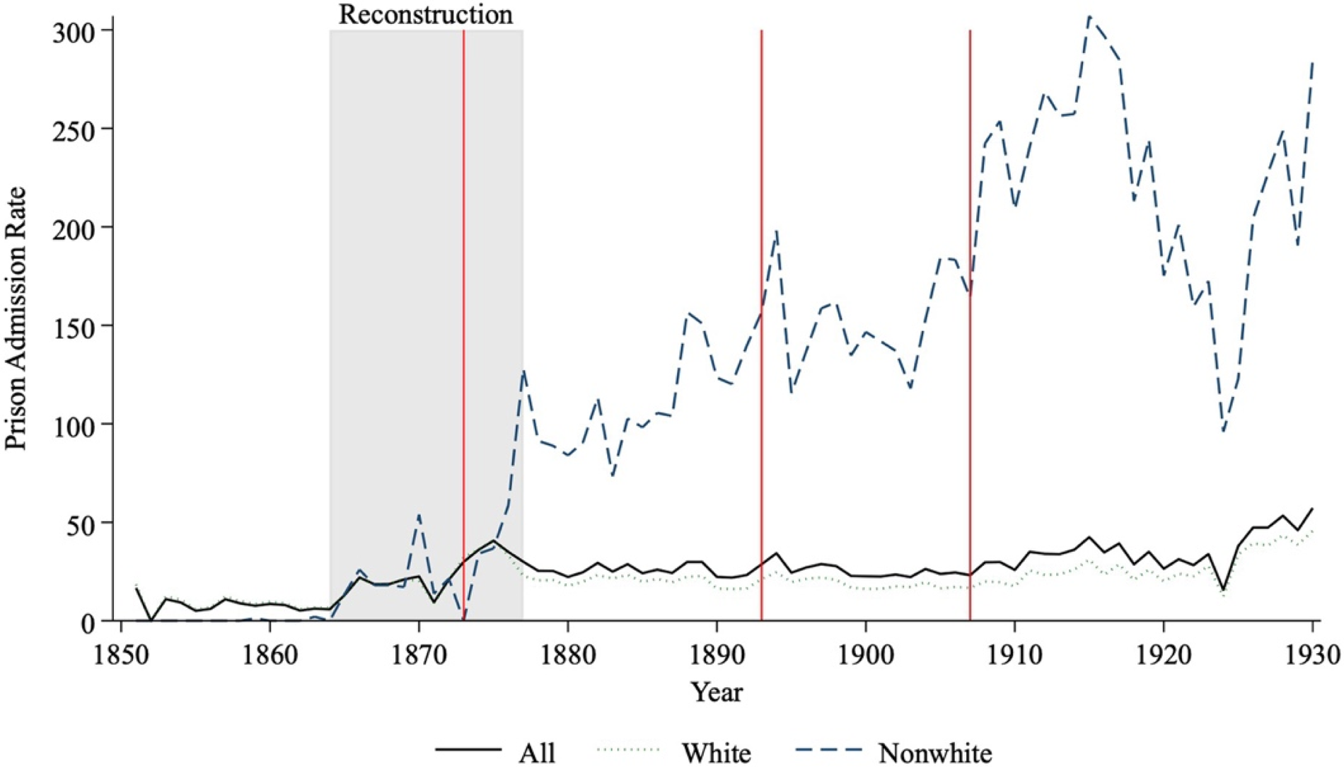
I start by documenting the broader patterns of incarcerated individuals’ backgrounds in post-bellum Missouri and demonstrate changes in the composition of the incarcerated population over time. I find that the racial gap in prison admission rates emerged immediately after Reconstruction.
To examine the relationship between economic conditions and incarceration, I construct exogenous shock measures to counties’ local economic conditions by leveraging exogenous national crop price fluctuations and the variation in counties’ suitability for different crops. These measures serve as the basis for examining the association between economic conditions and crime, as captured by prison admission rates. My empirical strategy is supported by two important historical realities. First, the agricultural market exhibited a high degree of national and even international integration during this period, rendering local farmers price takers. Therefore, national price shocks interacting with county-level crop suitability are essentially exogenous to each county (Fogel Reference Fogel1962). Second, before the Great Depression, there was little systematic government intervention in the agricultural market, resulting in high price volatility due to unstable politics in Europe and underdeveloped agricultural technology (Rothbard Reference Rothbard1972).
I find that prison admission rates were negatively related to price shocks, which would be expected if the propensity to engage in criminal activity responds to available economic opportunities. I find an effect across all crimes, in contrast to the literature on modern crime rates that finds responses for property crimes only (Raphael and Winter-Ebmer Reference Raphael and Winter-Ebmer2001; Gould, Weinberg, and Mustard Reference Gould, Weinberg and Mustard2002). The size of the effect depends on the direction of the shock, with economic downturns increasing crime rates more than similarly sized booms reduce them. In absolute terms, I find that the impact of agricultural price shocks is larger for Black admission rates than for white admission rates, but due to the higher average rate for Blacks, the proportional effect of price shocks is much larger for whites. My findings are robust to alternative specifications of the shock measures and are not driven by changes in the police force.
The remainder of the paper is organized as follows. The first section describes the historical background of the criminal justice system in the United States and the state of Missouri. The second section provides a conceptual framework for the relationship between economic conditions and incarceration. The third section describes the data. The fourth section presents the empirical strategy and empirical evidence on the relationship between economic conditions and incarceration. The fifth section discusses the findings and concludes.
BACKGROUND
The U.S. prison system was first established as penitentiary houses that featured “home-styled” environments with communal living, working, and lax security after the American Revolution. In the early 1820s, it was replaced by the “Auburn System,” in which incarcerated people were required to live in solitary confinement and keep silent while working in small workshops (McLennan Reference McLennan1999). The prison system saw more dramatic changes in the postbellum era, when more interaction among incarcerated people was allowed again, and convict labor became common. The burgeoning incarceration rates made the isolation of incarcerated individuals prohibitively expensive, and technological advancements in mechanization made it financially profitable for states to use prison labor in mass production (McKelvey Reference McKelvey1936).
The composition of the incarcerated population also experienced changes over U.S. history. While Black Americans are five times more likely to be incarcerated (Carson Reference Carson2021), this gap emerged long before the contemporary rise in national incarceration rates (Muller Reference Muller2012; Eriksson Reference Eriksson2019). Previous work using the Census of Prisons has shown that the gap had already emerged by the early twentieth century (Moehling and Piehl Reference Moehling and Piehl2009), and this paper further documents that the racial gap arose precisely after the end of Reconstruction. Moehling and Piehl (Reference Moehling and Piehl2009) used the Census of Prisons data and documented a relative decline in incarceration rates of the foreign-born population in the early twentieth-century United States, which was further documented in Abramitzky et al. (Reference Abramitzky, Boustan, Jácome, Pérez and David Torres2023) with full-count Census data.
Historical Context of Missouri
Missouri became a territory of the United States in 1803, after the Louisiana Purchase. Statehood followed in 1820 after the famous Missouri Compromise, which admitted Missouri as a slave state, but stated that the remaining portion of the Louisiana Territory above the 36°30′ line was to be free from slavery (Foley Reference Foley2014). Since then, different groups have migrated to and settled in Missouri in large numbers. Southern planters brought enslaved African Americans with them and built plantations along the Missouri River.Footnote 5 This “Black Belt” running from Kansas City to St. Louis has long served as the economic center of the state. Meanwhile, poor whites from the East Coast came to settle in the vast rural areas of Missouri, especially after the Homestead Act of 1862, while a large number of European immigrants settled in booming urban centers following the opening of major roads and railways along the Missouri River.
The mix of rural farms, plantations, and urban centers made Missouri diverse and representative of the United States during this period (Meyer Reference Meyer1982). Missouri has always been a battleground of ideology, mimicking the country as a whole. During the Civil War, Missouri was the only slave state that called a secession convention but voted not to secede from the Union, and the guerrilla warfare between the two sides persisted longer in Missouri than in any other state (Brownlee Reference Brownlee1983; Geiger Reference Geiger2010). In the postbellum era, no political party was able to dominate state politics, and Missouri served as a bellwether of U.S. politics for more than a century, due to the mix of immigrant groups, elite planters, and poor white farmers in its electorate (Harris Reference Harris1971; Anderson Reference Anderson2008).
After the Civil War, Missouri saw a long period of economic growth and diversification. Many different types of industries boomed, especially in urban centers along the Pacific Railroad. As a railroad nexus, St. Louis became the fourth largest city in the nation. Before Chicago took its place, St. Louis was the most important transportation hub in the United States and had the largest share of foreign-born population in the United States (Meyer Reference Meyer1982; Thelen Reference Thelen1986; Christensen and Kremer Reference Christensen and Kremer2004). At the same time, agriculture was still Missouri’s main economic sector: more than 70 percent of the population still worked in agriculture in 1900. However, the variety and scope of farming increased, as new crops such as wheat and corn became prominent. In 1900, farmers devoted more than 7.5 million acres (of nearly 23 million total) to corn, and areas such as the Bootheel in the southeastern part of Missouri were newly developed into farmland as irrigation improved (Mumford Reference Mumford1921).
Criminal Justice System in Missouri
PRISON SYSTEM
Missouri operated a dual-tier incarceration system: local jails held pre-trial defendants, while the state prison housed convicted felons and select misdemeanor offenders. I focus on state prisoners in this paper. The Missouri State Penitentiary, established in 1836 in Jefferson City, served as the state’s sole prison for over a century. The facility expanded to 47 acres over time, eventually becoming the nation’s largest prison with more than 2,000 inmates housed in segregated but centralized blocks (Johnson Reference Johnson1903). Its establishment served both to centralize the state prison system and legitimize the position of Jefferson City—then merely a settlement of 31 households—as state capital (Rasmussen Reference Rasmussen2012).
JUDICIAL SYSTEM
Unlike in most of the U.S. today, the justice system worked quickly in Missouri between 1870 and 1930. The median time between court appearance and sentencing was less than three months (see Figure C7 in Online Appendix C), which validates my use of admission dates as a proxy for the timing of the crime.
Convict labor is the practice of coercing incarcerated individuals to work for private companies or state entities with minimal or no compensation. While convict labor was commonplace in the postbellum United States (Poyker Reference Poyker2019), Missouri developed a distinctive approach after the 1880s. Rather than utilizing chain gangs or convict leasing like other Southern states, Missouri established private industrial operations within prison walls while maintaining direct state supervision (Kremer and Gage Reference Kremer and Gage1980).
This approach emerged from two distinct factors. First, Jefferson City’s small size meant prison labor comprised a significant portion of the workforce, sparking labor conflicts in the 1870s–1880s, particularly when authorities deployed prison labor to break strikes (Reynolds Reference Reynolds1982). Frequent escapes during external work assignments further intensified opposition to traditional chain gangs or convict leasing systems (Reynolds Reference Reynolds2019). Second, the prison’s status as one of the nation’s largest correctional facilities yielded an economy of scale. Concentrating workers in a single location minimized operational costs and provided a dependable workforce with limited turnover. After the state legislature outlawed chain gangs and direct convict leasing but favored private sector contracts within prisons in the 1880s, the Missouri State Penitentiary attracted multi-year contracts from the biggest companies in the country (Kremer Reference Kremer1992). This practice may have led to an opposing relationship between economic conditions and incarceration rates. Tighter labor markets due to positive economic shocks may have increased the demand for convict labor and created incentives to increase the incarcerated population, perhaps by increasing sentence lengths.
TESTING BECKER’S HYPOTHESIS IN A HISTORICAL CONTEXT
Becker (Reference Becker1968) pioneered the economic analysis of crime and argued that crime was affected by expected economic returns and the opportunity costs of punishment. Theoretically, opportunity costs consist of the earnings that are foregone due to incarceration. These forgone earnings are lower during economic downturns. Since then, a large empirical literature has examined the different determinants of crime, including deterrence (Apel Reference Apel2013; Lee and McCrary Reference Lee, McCrary and Matias2017), policing (Klick and Tabarrok Reference Klick and Tabarrok2005; Levitt and Miles Reference Levitt and Miles2006), prison (Levitt Reference Levitt1996; Johnson and Raphael Reference Johnson and Raphael2012), and economic conditions (Chalfin and Raphael Reference Chalfin, Raphael and Tonry2011; Chalfin and McCrary Reference Chalfin and McCrary2017).
Even though there is a large literature on the relationship between the local economy and crime, an empirical consensus has not been reached. Raphael and Winter-Ebmer (Reference Raphael and Winter-Ebmer2001) first used military contracts and state-specific oil costs as a source of identification and found a negative effect of unemployment on crime. Since then, economists have used different sources of exogenous economic shocks to identify the effect of local economic conditions on crime and incarceration (Fougère, Kramarz, and Pouget Reference Fougère, Kramarz and Pouget2009; Dix-Carneiro, Soares, and Ulyssea Reference Dix-Carneiro, Soares and Ulyssea2018). However, research in the United States setting has not reached an agreement on how responsive crime is to the local economy.
The challenge in identifying the causal relationship between economic conditions and crime is twofold.Footnote 6 Empirically, identifying local economic shocks proves to be difficult. Many common shocks, such as trade shocks, induce changes in public goods provision, which in turn change observed crime rates (Dix-Carneiro, Soares, and Ulyssea Reference Dix-Carneiro, Soares and Ulyssea2018). For example, numerous studies show that a larger police force deters crime in different contexts (Levitt Reference Levitt1997; Mello Reference Mello2019), complicating the separation of crime responses from economic shocks and policing adjustments. Moreover, the modern welfare state can soften the impact of economic shocks on crime (Deshpande and Mueller-Smith Reference Deshpande and Mueller-Smith2022), muting the opportunity-cost channel theorized by Becker (Reference Becker1968). As Chalfin and McCrary (Reference Chalfin and McCrary2017, p. 34) put it, “The estimates [of crime response to the local economy] remain sensitive to the time period studied.”
A large literature focusing on developed countries was unable to find strong relationships between the local economy and crime, as predicted by Gary Becker’s model of criminality (Draca and Machin Reference Draca and Machin2015), while this relationship is better established empirically in weakly institutionalized settings (Dell, Feigenberg, and Teshima Reference Dell, Feigenberg and Teshima2019). The empirical evidence in historical Missouri provides further evidence for the opportunity-cost channel, similar to findings in other weakly institutionalized settings.
To formalize the mechanism between local economic shocks and prison admissions, consider a simple model in which individuals expect a wage W in the labor market. I assume that the expected return Rj from crime type j and the probability of being convicted and incarcerated αj for crime type j are fixed. The expected loss to the individual is the opportunity cost of lost wages during the incarceration period if incarcerated, multiplied by the probability of incarceration,

An individual will choose to commit crime j if their expected net return is positive,

This means that there is a fixed reservation wage

for each crime type j, so that individuals whose wage W falls under the reservation wage

will find it optimal to commit crime j. The prison admission rate for crime j in the population is

In economic downturns, the share of people whose wages fall under the reservation wage
 will increase, and the corresponding prison admission rate pj will increase for every crime type j.
This framework implies that negative economic shocks, in the form of decreasing agricultural commodity prices, will reduce the opportunity cost of crime and increase prison admission rates. Similarly, positive shocks, all else being equal, will have the opposite effect and decrease prison admission rates.
Previous research has utilized prison records data to study historical incarceration in other countries.Footnote 7 The most closely related study is Archibong and Obikili (Reference Archibong and Obikili2023), which examines how economic shocks, induced by agricultural export price shocks, affected prison admissions in colonial Nigeria. They find that when prisons relied on convict labor, prison admission rates were procyclical, whereas they were countercyclical when convict labor was abolished after the end of colonial rule. In this setting, positive economic shocks raised demands for coerced prison labor, driving up the enforcement intensity αj rather than increasing the opportunity-cost W.Footnote 8 This framework is enabled by the fact that policing and prisons were both under colonial supervision and closely coordinated.
In contrast, in postbellum Missouri, state prisons did not control local enforcement. Local police, funded and overseen by municipal governments rather than state agencies, conducted arrests independently of the penitentiary system. The county and municipal governments did not benefit from sending inmates to state prisons.Footnote 9 Consequently, Missouri state prisons had little ability to increase enforcement intensity αj in response to changes in labor demand. However, the existence of convict labor in Missouri means that tighter labor markets due to positive economic shocks can create incentives to increase the incarcerated population size. One way state criminal justice agencies in Missouri could achieve this is by adjusting sentencing lengths. Under the labor demand mechanism, positive economic shocks can lead to longer sentences, which will expand the incarcerated labor force to meet shifts in demand for coerced prison labor.
I test the predictions of my framework using the data described in the third section and the empirical strategy outlined in the fourth section.
DATA
Incarceration Data
My primary data on incarceration are derived from digitized administrative records of the Missouri State Penitentiary, covering the entire population of prison inmates in Missouri between 1850 and 1931. All individuals who became part of the Missouri State Prison system are covered by the data. This excludes people who were incarcerated in county jails, which disproportionately incarcerated people for misdemeanor crimes. Because most of the imprisonment was in state and federal prisons at this time (Cahalan et al. Reference Cahalan and Parsons1986), this restriction does not threaten the validity of the analysis.Footnote 10 Moreover, incarceration in state prisons was usually much longer and less impacted by changes in the local police force, making it ideal for studying the relationship between the local economy and crime.
In the main analysis, I use information on demographic characteristics (race, gender, and age), geographical background (county of conviction, place of origin), and criminal justice system information (date of court assignment, prison admission, prison release, and sentence length). The dataset covers 62,127 individuals, and after rigorous data cleaning,Footnote 11 only 5.8 percent of observations were dropped, affirming the exceptional completeness of my full-count incarceration data. I provide further insights into the descriptive analysis later and comprehensive details on the data cleaning process in Online Appendix A. The data and code used in the analysis are available at Wu (Reference Wu2026).
My data allows me to overcome two main limitations in previous studies. First, existing data sources only provide a snapshot of the prison population at a given time, and this is not sufficient for studying incarceration changes on granular geographic and temporal dimensions. For example, the Census occurs only every ten years and does not provide information on the county of residence before incarceration. Second, we know less about the characteristics of incarceration in the second half of the nineteenth century. The group quarter status in the Census during this period uses inconsistent definitions (see Eriksson (Reference Eriksson2020) for discussion), and researchers have relied on other information to infer incarceration status during this period (Eriksson Reference Eriksson2019, Reference Eriksson2020). By introducing novel data, this paper provides further insight into the characteristics of the criminal justice system in the postbellum United States.
Decennial Census
I draw on anonymized full-count U.S. Census data from 1850 to 1930 (Ruggles et al. Reference Ruggles and Nelson2024; Ruggles et al. Reference Ruggles and Flood2020) and county-level characteristics compiled by Haines (Reference Haines2010) to obtain county-level demographic and economic characteristics (Ruggles et al. Reference Ruggles and Nelson2024; Ruggles et al. Reference Ruggles and Flood2020). For each county, I derive the following demographic variables: the proportion of the Black population, the proportion of the immigrant population, the proportion of the urban population,Footnote 12 the number of police officers, and the proportion of working-age men engaged in agricultural sectors.Footnote 13 Since the Census data are available only every ten years, and annual variation is required for my empirical analysis, I linearly interpolate county-level demographic information for the intercensal years.
Agriculture Data
I use the Census of Agriculture (Haines Reference Haines2010; Haines, Fishback, and Rhode Reference Haines, Fishback and Rhode2018) to collect information on the composition of agricultural production within counties. This data includes the output for each type of crop and the total value of land, all at the county level. The Census of Agriculture was typically conducted every ten years at the beginning of the decade, with an additional survey conducted in 1925.Footnote 14
To determine the annual average prices for each crop, I refer to the Historical Statistics of the United States (Carter et al. Reference Carter2006).Footnote 15 I normalize the unit of measurement between production data from the Census of Agriculture and price data from the Historical Statistics, enabling calculations of the value of each crop output.
LOCAL ECONOMY SHOCKS AND INCARCERATION
Evolution of Incarceration in Missouri
To illustrate the evolution of the criminal justice system in Missouri, Figure 1 shows the prison admission rates in Missouri between 1850 and 1930. Following the Civil War, prison admission rates experienced a notable spike; however, they maintained a consistent level over the subsequent 50 years, punctuated by significant year-to-year fluctuations. The prison admission rate was around 30 per 100,000 people between 1880 and 1930. This number is comparable to the only other estimate of prison admission rates in the postbellum United States.Footnote 16 The three vertical red lines represent three early economic panics within the data period, and a noticeable short-term increase in prison admission rates is evident after each economic crisis, suggesting a link between the economy and incarceration.Footnote 17
PRISON ADMISSION RATE BY RACE, 1850–1930
Notes: This graph shows the prison admission rate by year in Missouri between 1850 and 1930. The prison admission rate on the y-axis is defined as the number of prison admissions per 100,000 people. The three vertical lines mark the three major economic crises during this period: the Panic of 1873, the Panic of 1893, and the Panic of 1907. The gray shaded area represents the Reconstruction period.
Sources: Missouri State Penitentiary records, 1850–1931; Historical, Demographic, Economic, and Social Data: The United States, 1790–2002 (Haines Reference Haines2010).

Figure 1 also displays the time series of prison admission rates by race. Three patterns stand out. First, there was a sharp surge in Black incarceration post-Emancipation, contrasting the absence of Black individuals within the prison system during the 1850s when slavery was still legal in the United States. This absence is because slaveholders depended on enslaved people’s labor and had economic incentives to keep enslaved people out of the state prison systems by resolving crimes committed by enslaved individuals outside the jurisdiction of the criminal justice system (Muller and Schrage Reference Muller and Schrage2021; Muller Reference Muller2021). After the end of Reconstruction in 1877, Black prison admission rates drastically rose, surpassing those of whites and aligning with theories that the carceral state succeeded slavery as a system for racial control (Weaver Reference Weaver2007; Alexander Reference Alexander2010; Blackmon Reference Blackmon2008). Second, the prison admission rates of Black Americans fluctuated at very high levels post-Reconstruction. Throughout the first three decades of the twentieth century, the prison admission rate for the Black population was around 200 per 100,000, already surpassing global contemporary levels. For comparison, in 2021, the U.S. imprisonment rate was 358 per 100,000 (Carson Reference Carson2021), while Canada and China stand at 90 and 119, respectively (Fair and Walmsley Reference Fair and Walmsley2024). Third, the racial gap in prison admission rates persisted after Reconstruction at levels comparable to the modern rates. After the 1880s, the prison admission rates for Black population were more than six times the rate for white population, paralleling modern statistics of Black-to-white incarceration ratios of 5.5 (Neal and Rick Reference Neal and Rick2014; Carson Reference Carson2021). This resemblance underscores enduring racial inequalities within the U.S. criminal justice system.
GEOGRAPHY OF INCARCERATION
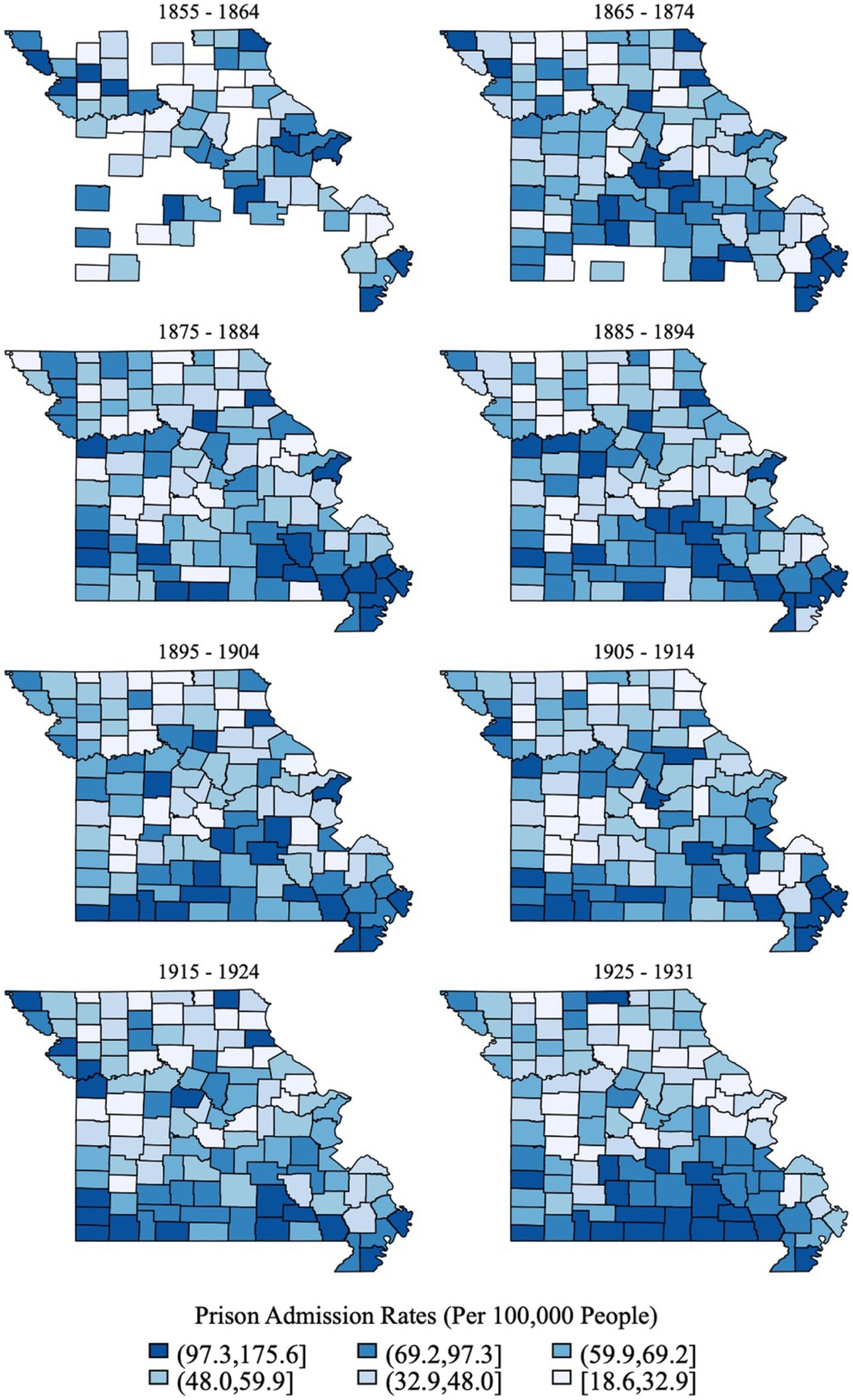
Figure 2 shows the map of average prison admission rates at the county level for each decade. Darker colors indicate a higher prison admission rate for the county. I group every ten years into one decade and calculate the average annual rate of prison admission. There is substantial variation both across decades and across counties.
GEOGRAPHIC DISTRIBUTION OF PRISON ADMISSIONS IN MISSOURI
Notes: This graph shows the map of prison admission rates by county for each decade between 1860 and 1930. The prison admission rate is defined as the average number of prison admissions per 100,000 people in a decade. A darker color means higher prison admission rates. Missing values for some counties in earlier years are attributed to the low prison admission rates and small populations before Reconstruction.
Sources: Missouri State Penitentiary records, 1850–1931; Historical, Demographic, Economic, and Social Data: The United States, 1790–2002 (Haines Reference Haines2010).

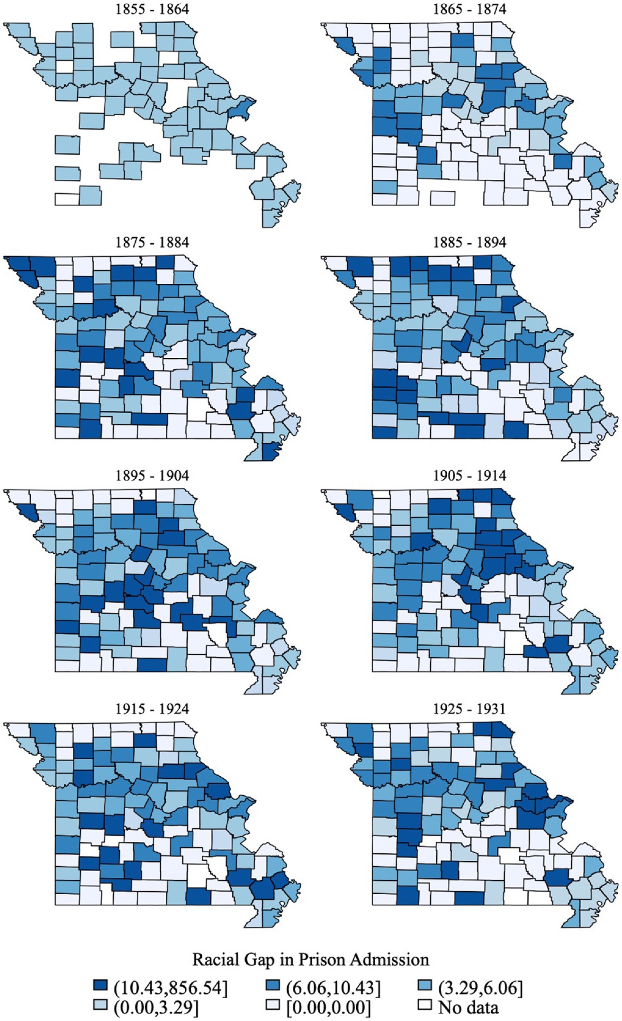
How did the racial difference in prison admission rates vary across counties within Missouri? Figure 3 shows the geography of racial gaps in each decade. I define the racial gap as how many times more likely a Black person was to be incarcerated than a white person in the same county. The racial gap was higher in the Northern part of the state, where the overall prison admission rate was lower and the economy was booming.
RACIAL GAP IN PRISON ADMISSION RATES IN MISSOURI
Notes: This graph shows the racial gap in prison admission rates by county for each decade between 1860 and 1930. The prison admission rate is defined as the average number of prison admissions per 100,000 people in a decade, and the racial gap is defined as the ratio between Black prison admission rates and White prison admission rates. A darker color means a larger racial gap in prison admissions. Missing values for some counties in earlier years are attributed to the low prison admission rates and small populations before Reconstruction.
Sources: Missouri State Penitentiary records, 1850–1931; Historical, Demographic, Economic, and Social Data: The United States, 1790–2002 (Haines Reference Haines2010).

AGE AND GENDER DISTRIBUTION OF INCARCERATION
The prison population tended to be made up of more men and youth than the general population. During the period of focus for this study, 97.8 percent of the incarcerated people were men. For the rest of the paper, I limit my focus to male inmates.Footnote 18 People under 30 accounted for the majority of prisoners, which is similar to patterns today (Kaeble et al. Reference Kaeble2016).
CRIME TYPES
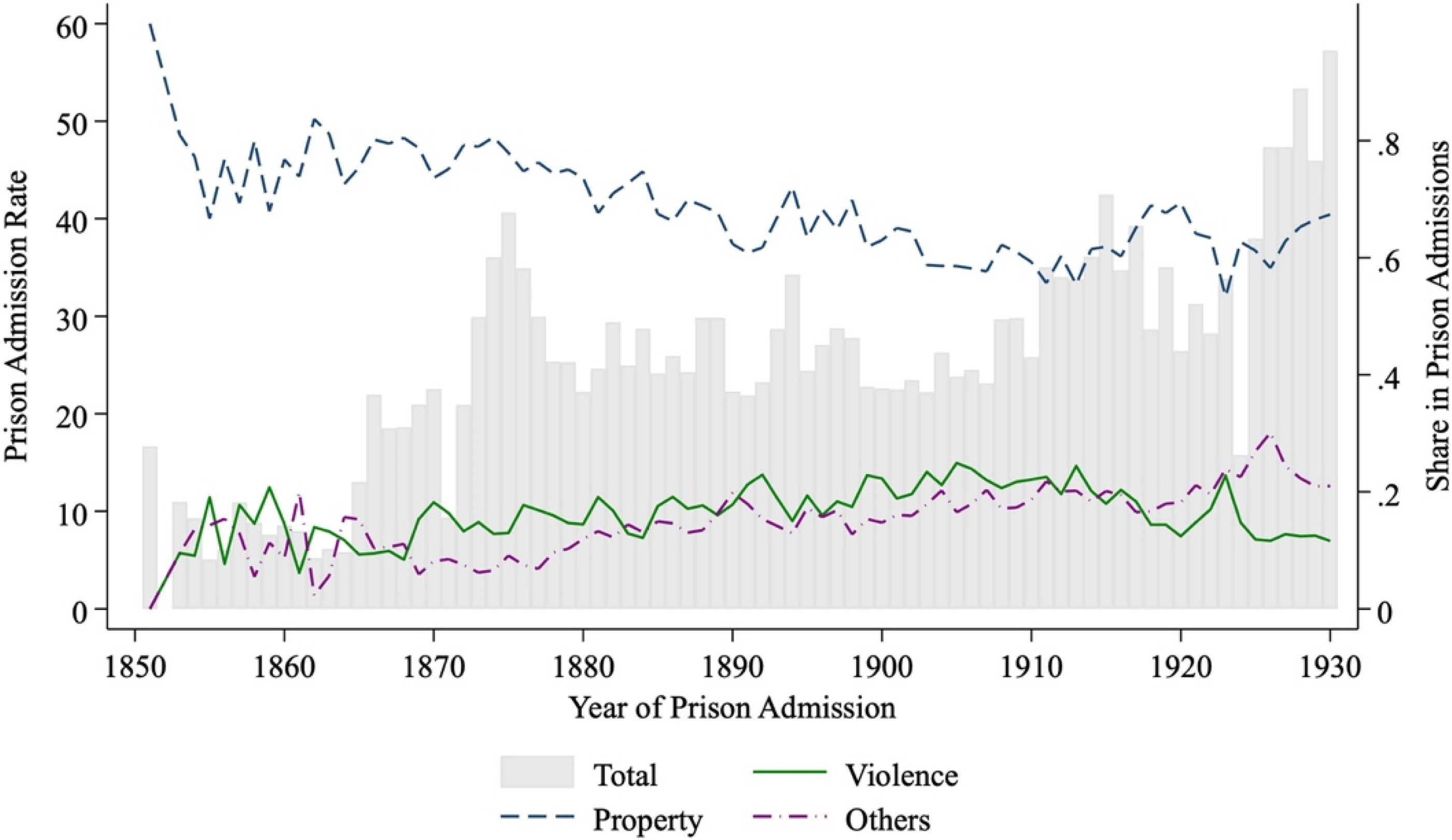
Different types of crimes leading to incarceration can have economically meaningful differences in their causes and implications. Figure 4 shows the composition of crimes by offense type throughout the period. I code crimes into three categories: violent crimes,Footnote 19 property crimes,Footnote 20 and other crimes, most of which were about disobeying social orders.Footnote 21 Property crimes comprised half of all crimes during this period, but the percentage gradually decreased from 60 percent in the 1850s to 45 percent in the 1920s. On the other hand, there was a gradual increase in violent crimes and other crimes. Note that the spike in other crimes during the 1860s was driven by military prisoners during this period (Sanders Reference Sanders2005). Missouri was a battleground state under the control of the federal government, and it took federal troops several more years to eliminate the guerrilla warfare organized by Confederate sympathizers in rural Missouri (Geiger Reference Geiger2010). For this reason, when studying the relationship between the economy and crime, I limit the analysis to time periods after 1870.
PRISON ADMISSION RATE BY OFFENSE TYPE ACROSS YEARS
Notes: This graph shows the prison admission rate in Missouri between 1850 and 1930 for different crime types. The y-axis on the left corresponds to the prison admission rate, defined as the number of prison admissions per 100,000 people. The shaded area denotes the total prison admission rate among all crime types. Three lines referring to the y-axis on the right represent the share of total prison admissions for violent crimes, property crimes, and all other crimes.
Sources: Missouri State Penitentiary records, 1850–1931; Historical, Demographic, Economic, and Social Data: The United States, 1790–2002 (Haines Reference Haines2010).

Empirical Strategy
I leverage fluctuations in each crop’s national price and account for the varying susceptibility of each county to such price changes to construct measures of local economic shocks at the county-year level. Intuitively, the magnitude of these shocks depends on three factors. First, it depends on the extent to which the economy of a county relied on agricultural production. Second, it is influenced by the significance of a particular crop in the county’s overall agricultural output. Lastly, it is determined by the extent of price fluctuations observed for each crop in a given year.
IMPORTANCE OF AGRICULTURE
The first part of the variation comes from the importance of agriculture in the overall economy. Counties more dependent on agriculture would be more affected by agricultural shocks of the same scale. I leverage the variation in the reliance on agriculture and proxy this by the share of working-age men who work in agriculture from the Census data. Because this information is only available every ten years, I proxy the annual level by interpolating between years.
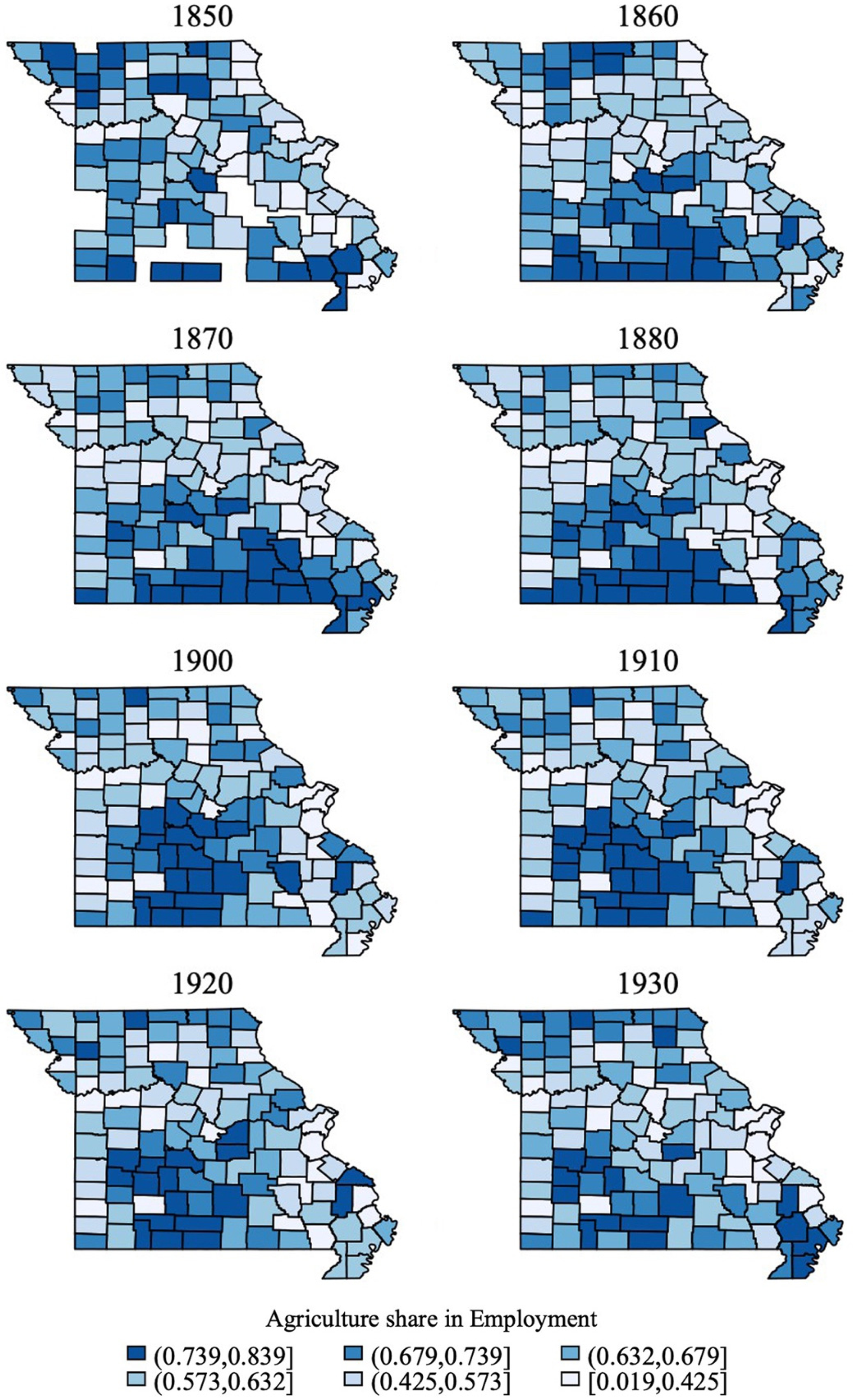
While there was an overall decline in the importance of agriculture, a substantial proportion, ranging from 30 percent to 60 percent of the total working population, still engaged in farming during this period. This decline is driven by an increase in employment in other sectors; total agricultural employment increased between 1860 and 1900 and remained stable after 1900 (see Figure C3 in Online Appendix C). However, this aggregate trend masks an even greater significance of agriculture in rural counties. In Figure 5, we observe the spatial distribution of the agricultural share across counties and over time. Remarkably, even at the end of my data period in 1930, the median county still had 70 percent of working-age men employed in agriculture.Footnote 22 Consequently, not only did geographic differences exist in the initial significance of agriculture, but counties also diversified at varying paces.
GEOGRAPHIC DISTRIBUTION OF AGRICULTURAL EMPLOYMENT IN MISSOURI
Notes: This graph shows the map of agricultural employment share by county for each decade between 1850 and 1930. The agricultural employment share is defined as the share of all employed population in agricultural sectors in Censuses.
Sources: IPUMS Full Count Census Data, 1850–1930 (Ruggles et al. Reference Ruggles and Flood2020; Ruggles et al. Reference Ruggles and Nelson2024).

AGRICULTURE COMPOSITION
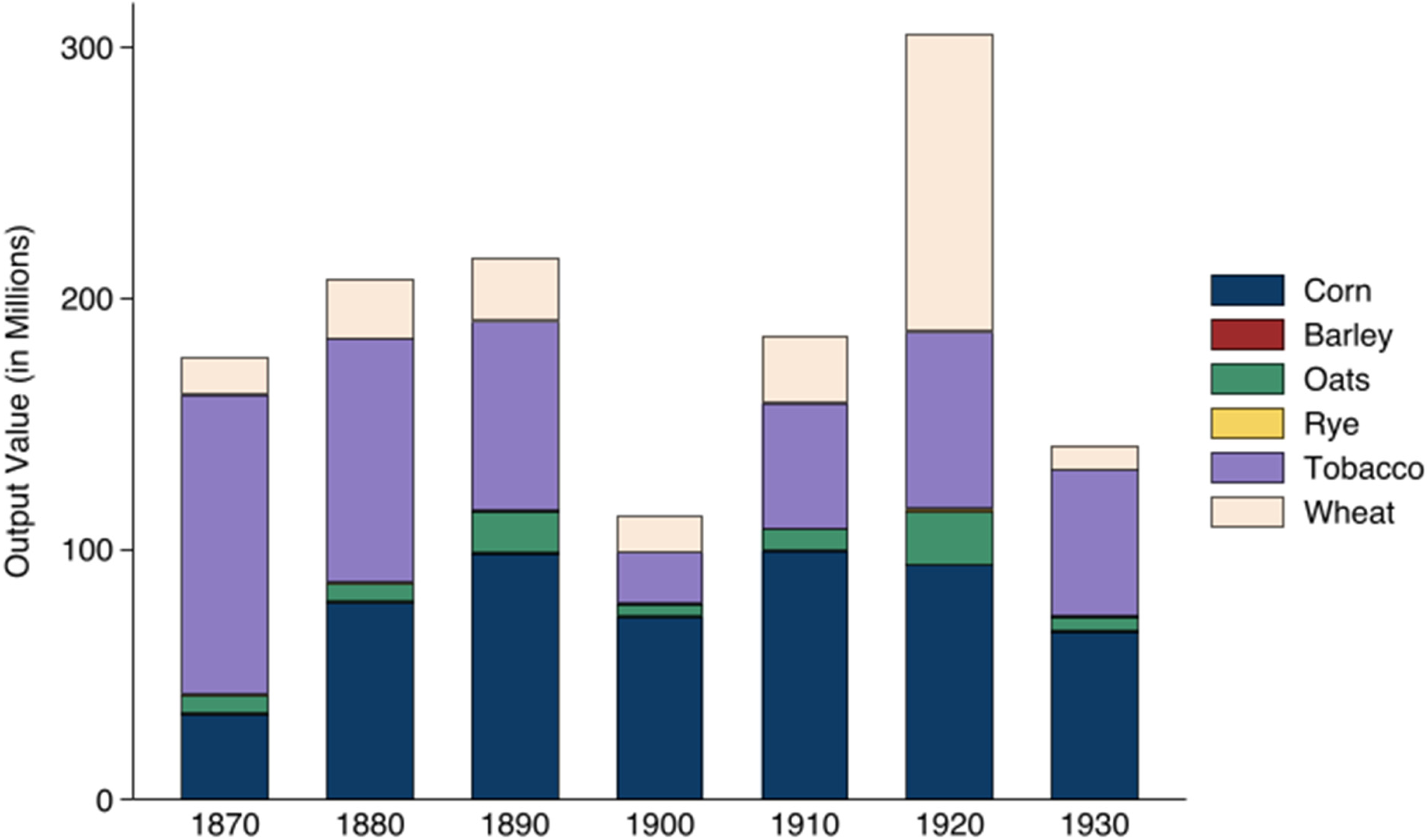
The second part of the variation comes from heterogeneity in the crop composition of counties. When the price for one crop decreases, it disproportionately hurts counties that specialize in producing this crop before the shock. Figure 6 shows the total output value of the six main crops with consistent data coverage throughout the period. Four crops alone accounted for most agricultural production: corn, oats, wheat, and tobacco. In all the following empirical analyses, I focus on these four crops to construct shock measures. Figure C4 in Online Appendix C also shows the share of these four crops’ output out of the total land value in Missouri. These four crops comprised around 30 percent of the total land value in Missouri, giving me confidence that omitting other crops from my analysis is unlikely to threaten the validity of my results.
COMPOSITION OF MISSOURI AGRICULTURAL OUTPUT
Note: This graph shows the time series of total agricultural output in Missouri for six main crops: corn, barley, oats, rye, tobacco, and wheat.
Sources: United States Agriculture Data, 1840–2012 (Haines, Fishback, and Rhode Reference Haines, Fishback and Rhode2018); Historical Statistics of the United States (Carter et al. Reference Carter2006).

One major challenge in identification is that the composition of agricultural output might endogenously adjust to market conditions. When prices for corn change, for example, farmers might switch to farming wheat instead. However, due to characteristics of the natural environment, such as the soil and climate, the extent of this adjustment is limited, at least in the short run. Figure C5 in Online Appendix C shows the share of each crop in a county’s output value over decades, and the pattern persists across years. Therefore, by fixing the agricultural composition at a prior level, I control for endogenous changes and separate the more permanent determinants of crop specialization in each county.
Choosing when to measure crop specialization involves a trade-off. If the previous year is too close to the actual year’s price shocks, my crop composition measure might capture anticipated adjustments, especially for long-lasting shocks that extend beyond a year, such as WWI. Additionally, annual county-level observations of agricultural output are not readily available. Conversely, if the prior year is too far back in time, my measure might miss substantial variation from secular changes in agricultural development at the aggregate level. To strike a balance, I measure the composition of production in the Census taken at the beginning of each decade. This approach utilizes precisely measured data from the Census of Agriculture and captures secular changes over the 60 years of study. I operationalize this measurement as Share ij,t−mod(t,10). Additionally, I construct three alternative measures by choosing prior periods farther back in time, resulting in more conservative estimates, since they may capture a crop composition that is less relevant to the time period when the shocks occur. I provide detailed specifications in Online Appendix B and show that my main results remain robust to these alternative approaches.
CROP PRICE SHOCK
The third source of variation comes from national agricultural price shocks. The agricultural market in the United States was very integrated by the end of the nineteenth century, mostly due to the expansion of railroads across the country (Fogel Reference Fogel1962). I use annual crop price data from the Historical Statistics of the United States.
My identifying assumption is that prices were exogenous to each county. This means that a county’s economic situation cannot directly affect the national price in any way. Situated at the intersection of railroad networks nationwide, Missouri transported most of its crops out of state and sold them to the national market. Therefore, national prices determined the value of farmers’ agricultural output during this period.Footnote 23 A straightforward way to validate this assumption is to examine how important Missouri was in national production. Figure C6 in Online Appendix C shows Missouri’s share of national output for each Census year. The total farm production value never exceeded 6 percent of the national aggregate, and for the four crops analyzed, this percentage never exceeded 12 percent in any year, remaining below 6 percent for most years. The decentralized production network makes collusion between counties highly improbable. Without substantial market power or collusion in an integrated market, Missouri’s counties can be considered price takers, as their economic and social changes have no effect on national prices.Footnote 24
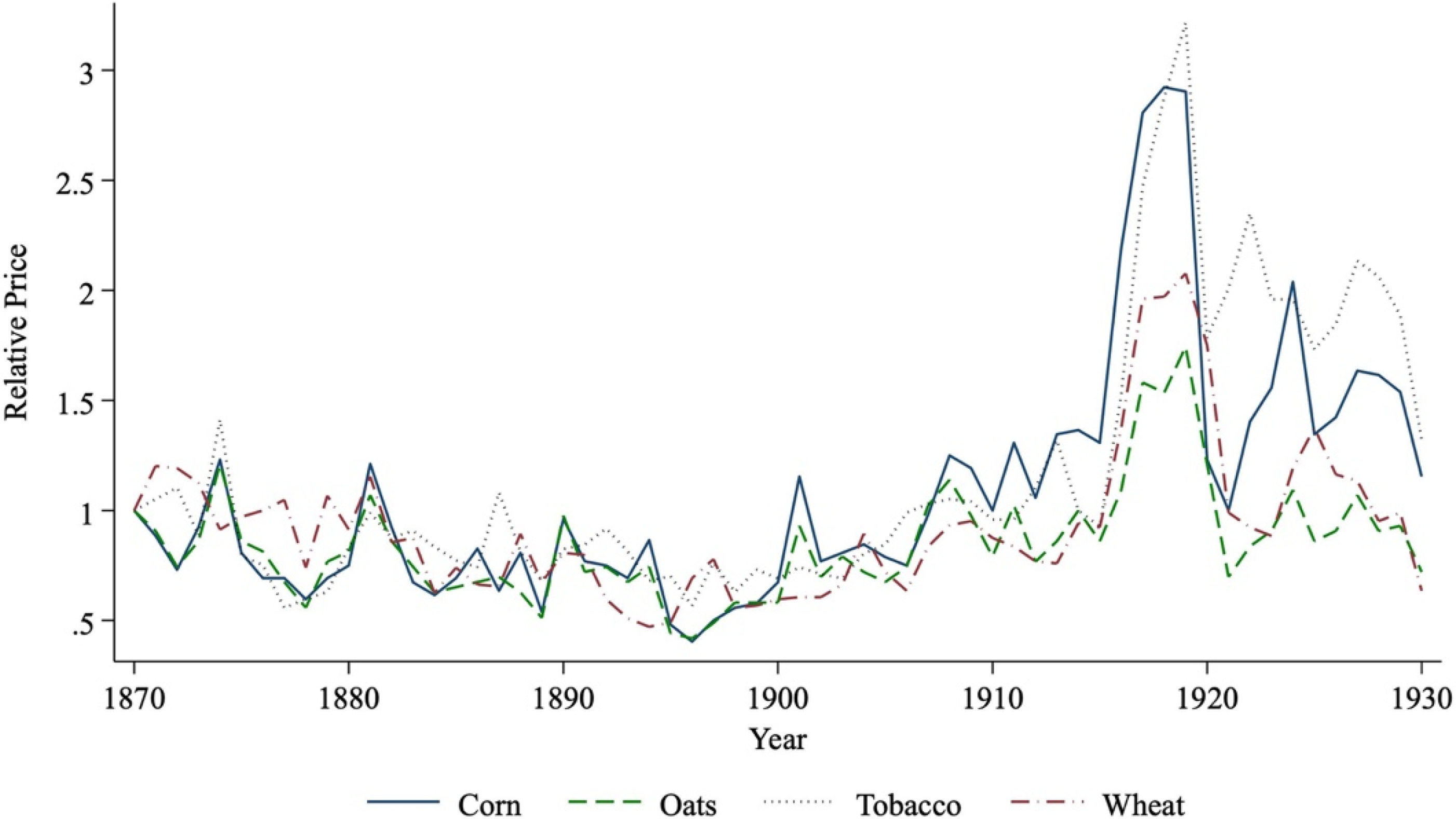
Figure 7 shows the time series of prices for the four main crops during this period, with all prices normalized to one in 1870. Significant price swings from year to year provide the necessary variation for my analysis. Laissez-faire principles dominated the political and economic landscape during this period, with minimal regulation on agricultural markets (Rothbard, Reference Rothbard1972; Gordon, Reference Gordon2017). While prices for different crops were highly correlated, especially during the disruptions caused by WWI in the 1910s, substantial within-year differences across crops remained. For instance, during WWI, corn prices fluctuated much more than tobacco prices. Since I include year fixed effects, the identifying variation stems from the differences in price changes across crops in the same year.Footnote 25
NATIONAL CROP PRICES, 1870–1930
Note: This graph shows the national average prices for corn, oats, tobacco, and wheat. All prices are normalized to the 1870 price level.
Sources: Historical Statistics of the United States (Carter et al. Reference Carter2006).

Shock Measurements
Based on the factors discussed previously, I formulate my shock measure as:

where i indexes crops, j denotes county, and t denotes year. AgriSharejt is the share of working-age men employed in agriculture interpolated from the decennial Census, while PriceShockit denotes the percentage changes in prices compared to the Census year, and Share ij,t−mod(t,10) denotes the share of crop i in county j’s crop bundle output in the Census year in which I measure agricultural composition.
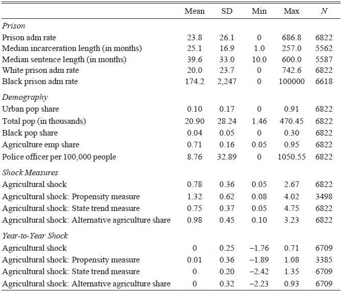
By construction, AgriculturalShockjt simulates the relative change in the economy by price shocks alone, with the Census year level normalized to one. The third and fourth panels of Table 1 show summary statistics for the agriculture shocks I construct. There is substantial variation in the agricultural price shock measure, facilitating my empirical strategy. There are still significant changes in output price when I narrow down to year-to-year changes, showing that the results in this paper are not driven by any single shock event.
COUNTY-LEVEL DESCRIPTIVE STATISTICS

Notes: This table shows the summary statistics for the variables used to estimate Equation (2). The first panel describes the prison admission rates constructed from the dataset. Prison admission rates are defined as the number of prison admissions per 100,000 people in a given year. The second panel describes the demographic characteristics of counties in Missouri. The third panel describes the agricultural shock from crop price fluctuations, as defined in the fourth section and Online Appendix B. The fourth panel describes the year-to-year change in agricultural shocks.
Sources: Missouri State Penitentiary records, 1850–1931; Historical, Demographic, Economic, and Social Data: The United States, 1790–2002 (Haines Reference Haines2010); United States Agriculture Data, 1840–2012 (Haines, Fishback, and Rhode Reference Haines, Fishback and Rhode2018); IPUMS Full Count Census Data, 1850–1930 (Ruggles et al. Reference Ruggles and Flood2020; Ruggles et al. Reference Ruggles and Nelson2024); Historical Statistics of the United States (Carter et al. Reference Carter2006).
Agricultural price shocks function as macroeconomic shocks that affect income across the economy. While these shocks directly impact farmers and sharecroppers in Missouri whose incomes are dependent on crop sales, their effects permeate throughout the broader economic system (Johnson Reference Johnson1997). During periods of price depression, farms may reduce their demand for labor, and households may cut back on spending, leading to a decline in aggregate demand across multiple sectors. The widespread effects of agricultural shocks on income distribution in agrarian societies are well-documented in the literature (Collier Reference Collier2002; Wright Reference Wright1978; Grabrucker and Grimm Reference Grabrucker and Grimm2021) and are analogous to the macroeconomic impacts of oil price shocks in industrialized economies (Baumeister and Peersman Reference Baumeister and Peersman2013; Baumeister and Hamilton Reference Baumeister and Hamilton2019). Thus, our constructed measure of agricultural shocks effectively captures income fluctuations that affect criminal behavior through the economic opportunities channel, as theorized by Becker (Reference Becker1968).
Specification
With the shock measures I constructed, I estimate the following two-way fixed effect model:

where the outcome variable PrisonAdmissionjt denotes the number of prison admissions per 100,000 people in county j, year t. I construct this variable from the full-count incarceration data. AgriculturalShockjt denotes the agricultural shock measures defined in Equation (1). λt and σj represent the year fixed effects and the county fixed effects, respectively. Xjt includes a set of county characteristics, such as the urban share of the population, the Black share of the population, and the total population. The regressions are weighted by county population. I derive all these variables from the Census, and they are linearly interpolated for years between the Censuses.
Table 1 presents descriptive statistics for the variables included in this specification. Prison admission rates for Black people are significantly higher than those for white people and exhibit greater variance. This variance arises from the concentration of Black people in Missouri; across more than 25 percent of the counties, the Black population made up less than 0.5 percent of the total population, leading to smaller denominators. For the demographic variables, the analysis highlights Missouri’s predominantly rural and white composition. On average, a county in Missouri had a population of 21,000 during this period, with 10 percent of the population classified as urban and 4 percent as Black.
Baseline Results
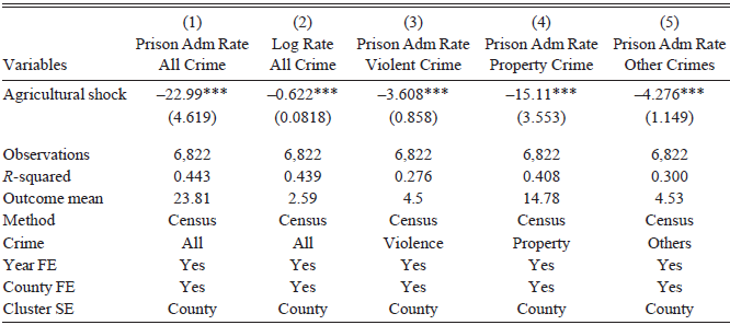
Table 2 shows my baseline results with the main specification. Column (1) presents standard two-way fixed effects estimates for the entire sample. The coefficient on the Black population share is significantly positive, even after controlling for county and year fixed effects. The effect of the agricultural price shock measure on incarceration is significantly negative. This means that a 10 percentage point positive shock to the economy from crop price shocks would lead the prison admission rate to decline by 2.3 per 100,000 people, a 9.7 percent decrease from the average prison admission rate of 23.81. Column (2) uses log-rate as the outcome variable to address concerns related to the fat-tailed distribution of the prison admission rates, and my results are robust to this change in functional form. The results indicate that prison admission rates are negatively associated with the strength of the economy.
EFFECT OF LOCAL ECONOMIC SHOCKS ON INCARCERATION

Robust standard errors in parentheses
*** p<0.01, ** p<0.05, * p<0.1
Notes: This table shows the effect of economic shocks on prison admission rates, as in Equation (2), with shock measurements constructed in the fourth section The dependent variable for Columns (1)–(5) is prison admission rate, log prison admission rate, violent crime admission rate, property crime admission rate, and all other crime admission rate, respectively. In all specifications, the dependent variable is the prison admission rate, with controls for total population, urban population share, Black population share, year fixed effects, and county fixed effects. Standard errors are clustered at the county level, and observations are weighted by total population.
Sources: Missouri State Penitentiary records, 1850–1931; Historical, Demographic, Economic, and Social Data: The United States, 1790–2002 (Haines Reference Haines2010); United States Agriculture Data, 1840–2012 (Haines, Fishback, and Rhode Reference Haines, Fishback and Rhode2018); IPUMS Full Count Census Data, 1850–1930 (Ruggles et al. Reference Ruggles and Flood2020; Ruggles et al. Reference Ruggles and Nelson2024); Historical Statistics of the United States (Carter et al. Reference Carter2006).
Columns (3)–(5) in Table 2 break down prison admission rates by the types of crimes prisoners committed. Across the three categories (violent crimes, property crimes, and other crimes), the strength of the local economy negatively impacted prison admission rates for all types of crimes. However, the coefficient is larger for property crimes than for violent crimes or other crimes. This is consistent with Becker’s (Reference Becker1968) theory that the economy impacts not only the opportunity cost of incarceration, but also the utility payoff (Rj) from property crimes. Previous literature has found similar patterns (Wong Reference Wong1995; Raphael and Winter-Ebmer Reference Raphael and Winter-Ebmer2001; Mehlum, Miguel, and Torvik Reference Mehlum, Miguel and Torvik2006).
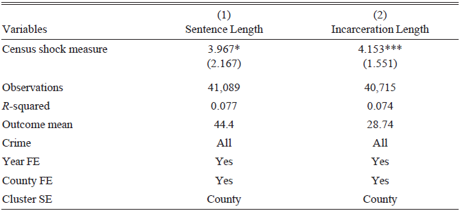
According to the conceptual framework in the previous section, the state criminal justice system had limited scope to respond to the changing labor demand on the extensive margin by adjusting prison admission rates, but could potentially respond on the intensive margin by varying sentence lengths. I find evidence supporting this hypothesis. Using individual-level data on prison admission dates, release dates, and sentencing information, I estimate the effect of economic shocks on sentence length and actual incarceration length, after controlling for a rich set of demographic information, including a quadratic of age, race, gender, and prior criminal history. I also include indicators for crime types to control for the severity of the crime and only compare the intensity of incarceration for similar offenses. In Table 3, I show that the agricultural price shock measure has a significantly positive effect on both sentence lengths and incarceration lengths. However, the magnitude is much smaller compared to the extensive margin on the prison admission rate. The magnitude implies that a 10 percentage point positive shock to the economy from crop price shocks would lead the sentence length to increase by 0.40 months, a 0.9 percent increase from the average sentence length of 44.4 months. Similarly, a 10 percentage point positive shock would lead the incarceration length to increase by 0.42 months, a 1.5 percent increase from the average incarceration length of 28.7 months. In comparison, a 10 percentage point positive shock to the economy would lead the prison admission rate to decline by 2.3 per 100,000 people, a 9.7 percent decrease from the average prison admission rate of 23.81.
EFFECT OF LOCAL ECONOMIC SHOCKS ON INTENSIVE MARGINS OF INCARCERATION

Robust standard errors in parentheses
*** p<0.01, ** p<0.05, * p<0.1
Notes: This table shows the effect of economic shocks on sentence lengths and incarceration lengths from Equation (2). The dependent variable is the incarceration length in Column (1) and the sentence length in Column (2). Both variables are in months and are constructed on the individual level from admission dates, release dates, and sentence lengths from the Missouri State Penitentiary records. All regressions include controls for a quadratic of age, gender, race, offense type, prior occupation type, an indicator whether they have been incarcerated before, year fixed effects, and county fixed effects. The standard errors are clustered at the county level.
Sources: Missouri State Penitentiary record, 1850–1931; Historical, Demographic, Economic, and Social Data: The United States, 1790–2002 (Haines Reference Haines2010); United States Agriculture Data, 1840–2012 (Haines, Fishback, and Rhode Reference Haines, Fishback and Rhode2018); IPUMS Full Count Census Data, 1850–1930 (Ruggles et al. Reference Ruggles and Flood2020; Ruggles et al. Reference Ruggles and Nelson2024); Historical Statistics of the United States (Carter et al. Reference Carter2006).
The period I study also saw the early expansion of the police force. Figure C9 in Online Appendix C shows the size of the police force in Missouri over time. The number of police officers per 100,000 people skyrocketed fivefold between 1870 and 1930. Moreover, this is not a phenomenon driven only by the rapid growth of St. Louis, but a trend across the entire state. Figure C10 in Online Appendix C shows the spatial distribution of police force per capita in Missouri for each decade. The police force expanded with time in all parts of Missouri.
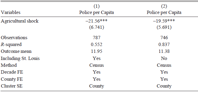
Substantial literature has shown that increasing the number of police officers can deter crime (Chalfin and McCrary Reference Chalfin and McCrary2018; Mello Reference Mello2019). Meanwhile, economic cycles can also affect tax revenues for local governments, altering the provision of local public goods (Rodrik Reference Rodrik1997; Feler and Senses Reference Feler and Senses2017). To test this mechanism, I control for police per capita as an independent variable in Equation (2). I calculate the size of the police force by counting the number of people recorded as police officers in the Censuses. Because we only observe the size of the police force every ten years in the Census data, I take the mean of the agricultural shock measures within the decade and implement the specifications at a county-decade level. Table D4 in Online Appendix D shows that accounting for the police force size does not meaningfully change the effect size of economic shocks on prison admission rates. This finding confirms that the effect of economic shocks on prison admission rates is not driven by changes in enforcement intensity.
To further examine the effect of local economic shocks on the size of the police force, I use the police per capita as the outcome variable (instead of prison admission per capita) and run the same specification in Equation (2). Table 4 presents my results from the police force regression analysis. In Column (1), we observe a negative impact of agricultural price shocks on police force size. I exclude counties within the St. Louis Metropolitan Statistical Area (MSA) in Column (2), given the dominant role of St. Louis in the total police force count, and the result remains robust. It is important to note that this mechanism could potentially attenuate the estimates provided in this paper, as a decrease in police force due to economic booms might lead to an increase in crime—counter to our primary finding. This pattern indicates that local governments had flexibility to adjust the police force size based on local demands, aligning with historical accounts that policing was less bureaucratized than it is today (Monkkonen Reference Monkkonen2004; Ornaghi Reference Ornaghi2019).
EFFECT OF LOCAL ECONOMIC SHOCKS ON POLICE FORCE

Robust standard errors in parentheses
*** p<0.01, ** p<0.05, * p<0.1
Notes: This table shows the effect of economic shocks on the size of the police force from Equation (2). The dependent variable is the number of police officers per 100,000 population in the Decennial Censuses. Column (2) excludes St. Louis MSA from the sample. All regressions include controls for total population, urban population share, Black population share, decade fixed effects, and county fixed effects. The standard errors are clustered at the county level, and the observations are weighted by the total population.
Sources: Historical, Demographic, Economic, and Social Data: The United States, 1790–2002 (Haines Reference Haines2010); IPUMS Full Count Census Data, 1850–1930 (Ruggles et al. Reference Ruggles and Flood2020; Ruggles et al. Reference Ruggles and Nelson2024).
Effect Heterogeneity
RACE HETEROGENEITY
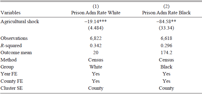
Table 5 shows the results separately for Black and white Missourians with the same specification. The outcome variable is the prison admission rates for white and Black populations in Column (1) and (2), respectively, and the control variables in Equation (1) are defined specifically for each race group. While the absolute effect of economic shocks on incarceration is larger for the Black population, the percentage change is approximately half that of the white population, reflecting the substantially higher baseline prison admission rates among Black Missourians.
EFFECT OF LOCAL ECONOMIC SHOCKS ON INCARCERATION: BY RACE

Robust standard errors in parentheses
*** p<0.01, ** p<0.05, * p<0.1
Notes: This table shows the effect of economic shocks on prison admission rates separately for White and Black populations, with shock measurements constructed in the fourth section. The dependent variable for Column (1) is the White prison admission rate, defined as the number of White prison admissions per 100,000 White population, and the Black prison admission rate in Column (2) is similarly defined. All regressions include controls for total population, urban population share, Black population share, year fixed effects, and county fixed effects. The standard errors are clustered at the county level, and the observations are weighted by the total population for the race group.
Sources: Missouri State Penitentiary record, 1850–1931; Historical, Demographic, Economic, and Social Data: The United States, 1790–2002 (Haines Reference Haines2010); United States Agriculture Data, 1840–2012 (Haines, Fishback, and Rhode Reference Haines, Fishback and Rhode2018); IPUMS Full Count Census Data, 1850–1930 (Ruggles et al. Reference Ruggles and Flood2020; Ruggles et al. Reference Ruggles and Nelson2024); Historical Statistics of the United States (Carter et al. Reference Carter2006).
The contemporaneous widening of the racial incarceration gap, therefore, cannot be explained by Black prison admissions being more sensitive to economic shocks than those of whites. More likely, higher Black incarceration was due to the general economic and social disadvantages of Blacks compared to whites after the Civil War. Newly emancipated Black Americans had far lower income and wealth than their white peers throughout the period (Smith and Welch Reference Smith and Welch1989; Bayer and Charles 2018; Derenoncourt et al. Reference Derenoncourt, Kim, Kuhn and Schularick2024). The enduring economic disadvantage likely contributed to higher Black prison admission rates, as did possible systemic discrimination and exploitation within the criminal justice system. Table D1 and Table D2 in Online Appendix D show the racial difference in the effect of economic shocks on sentence lengths and incarceration lengths, respectively. The positive relationship between economic conditions and incarceration intensity is much stronger for non-white individuals than for white individuals, suggesting that the economic incentives for coerced labor could potentially amplify the racial disparities in incarceration.
SHOCK DIRECTION HETEROGENEITY
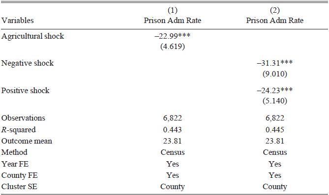
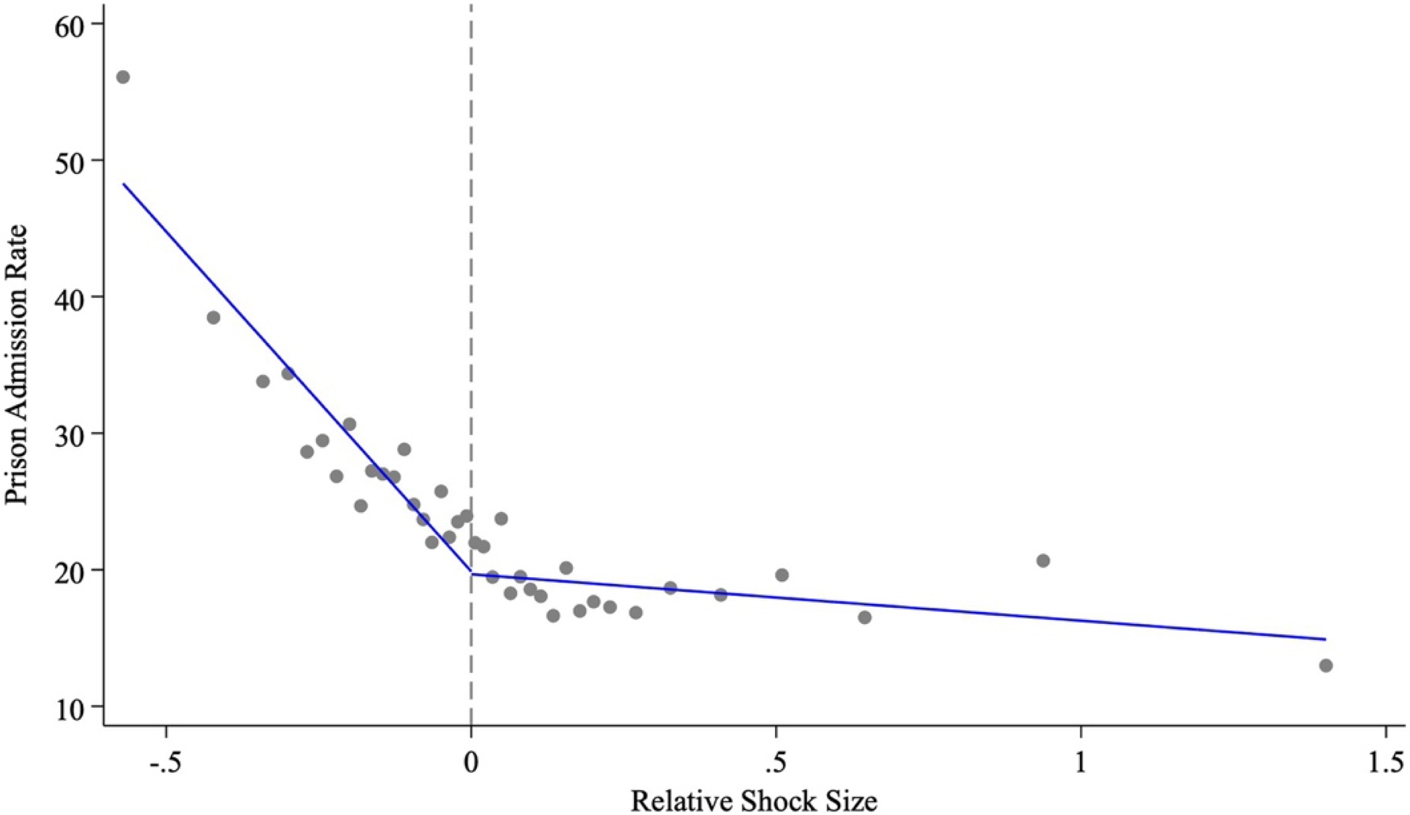
I test whether negative economic shocks and positive economic shocks have asymmetric effects on prison admission rates. I include measures separately for positive shocks and negative shocks in the same regression and test whether the coefficients on the two variables are significantly different. Table 6 Column (2) shows that the effect size is larger for negative shocks, and the difference in the coefficient magnitudes is statistically significant at the 90 percent confidence level. To visualize the relationship, Figure 8 shows a binned scatter plot of the prison admission rates and the agricultural shock size. It is clear that while there exists a negative relationship overall, the slope is steeper when the agricultural shock is negative.
EFFECT OF LOCAL ECONOMIC SHOCKS ON INCARCERATION: BY SHOCK DIRECTION

Robust standard errors in parentheses
*** p<0.01, ** p<0.05, * p<0.1
Notes: This table shows the effect of economic shocks on prison admission rates separately for positive shocks and for negative shocks. Positive shocks are defined as AgriculturalShockjt > AgriculturalShock j,t−1, and similarly for negative shocks. All regressions include controls for total population, urban population share, Black population share, year fixed effects, and county fixed effects. The standard errors are clustered at the county level, and the observations are weighted by the total population.
Sources: Missouri State Penitentiary records, 1850–1931; Historical, Demographic, Economic, and Social Data: The United States, 1790–2002 (Haines Reference Haines2010); United States Agriculture Data, 1840–2012 (Haines, Fishback, and Rhode Reference Haines, Fishback and Rhode2018); IPUMS Full Count Census Data, 1850–1930 (Ruggles et al. Reference Ruggles and Flood2020; Ruggles et al. Reference Ruggles and Nelson2024); Historical Statistics of the United States (Carter et al. Reference Carter2006).
BINNED SCATTER PLOT OF PRISON ADMISSIONS AND AGRICULTURAL SHOCK
Note: This graph shows a binned scatter plot of prison admission rates and agricultural shocks. The shocks are normalized to 0 so the positive shock implies an increase in crop production value. The prison admission rate is defined as the number of prison admissions per 100,000 people and the agricultural shock is defined as in Equation (1).
Sources: Missouri State Penitentiary records, 1850–1931; Historical, Demographic, Economic, and Social Data: The United States, 1790–2002 (Haines Reference Haines2010); United States Agriculture Data, 1840–2012 (Haines, Fishback, and Rhode Reference Haines, Fishback and Rhode2018); IPUMS Full Count Census Data, 1850–1930 (Ruggles et al. Reference Ruggles and Flood2020; Ruggles et al. Reference Ruggles and Nelson2024); Historical Statistics of the United States (Carter et al. Reference Carter2006).

The finding on the shock direction asymmetry is consistent with the literature on the slow recovery from economic downturns and unemployment scarring (Arulampalam, Gregg, and Gregory Reference Arulampalam, Gregg and Gregory2001; Fernald et al. Reference Fernald, Stock, Hall and Watson2017; Ikeda and Kurozumi Reference Ikeda and Kurozumi2019). In my conceptual framework, this phenomenon can be explained by the income distribution. For the reservation wage w ∗, anyone earning less than the reservation wage commits crime, and anyone earning more than it does not commit crime. When the density of the income distribution increases with wage near the threshold w ∗, the share below the reservation wage increases more when the distribution moves downward compared to the decrease when the distribution moves upward. I extend the conceptual framework in a formal model with the income distribution component in Online Appendix B.
Robustness
EXCLUDING ST. LOUIS
My results are robust to excluding St. Louis from all specifications. St. Louis was an outlier in Missouri for many reasons: While the rest of Missouri was rural and mostly homogeneous in terms of demographics, St. Louis was a booming metropolis with a large and diverse population base and fast-growing industries. St. Louis could drive the results in different directions. On the one hand, crime was mostly an urban phenomenon, so crime in urban areas might be especially susceptible to economic changes. On the other hand, urban populations were more likely to be buyers instead of sellers of crops; high agricultural prices would be a negative shock to their cost of living because they would need to spend more money on food. Whether St. Louis alone would bias the results is an empirical question. I drop the counties in the St. Louis metropolitan area and rerun the analysis as a robustness check.Footnote 26 Table D3 in Online Appendix D shows the results. Excluding St. Louis MSA does not change the magnitude or significance of my results.
ALTERNATIVE TEMPORAL MEASUREMENT
I use prison admission dates to construct annual prison admission rates in the main specification. To address potential timing discrepancies between crime commission and prison admission, I use alternative timing measures for crime. Figure C7 in Online Appendix C demonstrates that the interval between court assignment and prison admission was predominantly less than three months, and remained stable throughout the study period.Footnote 27 Additional analyses using court assignment dates in Table D5 and one-year lagged shock variables in Table D6, both in Online Appendix D, confirm the robustness of my main findings.
Additionally, I test whether the effect size differs by time of year. The cyclicality of agricultural production implies that crop price shocks are more salient right after the harvest, which usually falls in the third or fourth quarter of the year. I split the prison admissions based on the quarter of the year when the case was assigned to the court, which is close to the actual commission of the crime. Table D7 in Online Appendix D shows that the effect is largest in the fourth quarter, which confirms that the specification correctly captures the relationship between economic shocks and crime. Table D8 in Online Appendix D further demonstrates that my results remain robust when relying solely on decade-level variation, indicating that they are not influenced by the interpolation of demographic variables between Censuses. These consistent results across temporal specifications of incarceration suggest that timing measurements do not significantly affect my findings.
PRICE SHOCK FOR SINGLE CROP
The price shocks I construct are based on the bundle of four crops. To see whether this aggregation is driving the results, I reconstruct price shocks but use only one crop at a time and carry out the same empirical analysis. Table D9 in Online Appendix D shows the results for four single crop price shocks. The coefficients on the shock measures in Columns (2)–(5) are all negative, consistent with the baseline result in Column (1). This shows that prices for all four crops affected incarceration in the same way, which lends more confidence to my overall results.Footnote 28
ALTERNATIVE AGRICULTURAL SHARE MEASURE
I use the employment share of working-age men in the agricultural sector to capture the variation in reliance on agriculture in each county. Since fluctuations in the crop market could influence labor supply and occupational choices, I consider alternative measures of agriculture’s share in the economy. I replace AgriSharejt in Equation (1) with the proportion of total farm value relative to the combined total farm value and total manufacturing output from the Censuses and conduct the same empirical analysis. As shown in Table D10 in Online Appendix D, the estimated effects remain robust in both direction and magnitude when using this alternative measure.
ALTERNATIVE SHOCK MEASURE
I fixed the agricultural composition to that observed in the Census year at the start of the decade to control for endogenous adjustment. As a robustness check, I use other periods to measure baseline crop composition. First, I fix all agricultural composition to its 1870 level, the beginning of the study period, and extrapolate crop share based on the state aggregate trend. As shown in Table D11 in Online Appendix D, all coefficients remain negative and statistically significant. The alternative shock measure yields a smaller coefficient than the baseline, consistent with the fact that fixing the composition further back in time weakens the instrument for future crop composition, as technological change led to substantial changes in both agricultural production and crop composition over the subsequent 60 years (see Figure 5; Figure C5 in Online Appendix C). Second, I split the data into two periods, and instead of fixing the composition to the previous Census year, I fix it to the average composition in the first 30 years (1870–1900) and run the same specification only on the second 30 years of the sample (1901–1930). The results remain robust and consistent, as reported in Table D11 in Online Appendix D. Details of the specification can be found in Online Appendix B.
CONCLUSION
In this paper, I study the economic drivers of incarceration in the postbellum United States using state prison admission records from Missouri State Penitentiary. The unique full-count administrative data of the prison system over 80 years uncover new patterns of incarceration in U.S. history. I find that racial disparities in incarceration grew immediately after the end of Reconstruction, and the level is similar to modern estimates of the racial gap in incarceration. This persistence is in line with models that predict the continuance of inequalities given historical injustice (Derenoncourt et al. Reference Derenoncourt, Kim, Kuhn and Schularick2024).
In addition to describing the evolution of incarceration in Missouri with these detailed data, I further examine the relationship between local economies and incarceration. I first build a conceptual framework that incorporates individuals’ economic returns and opportunity costs from crime, and then build an empirical strategy to exploit the exogenous crop price fluctuations to estimate the causal effect of local economic conditions on prison admission. My empirical strategy relies on the fact that counties across Missouri specialized in different crops, and combines this variation with national price fluctuations for each crop over time. My findings show that counties with more negative price shocks experienced higher prison admission rates. This effect was present across all crime types but was more pronounced for property crimes and was stronger for negative shocks than for positive shocks. Both patterns are consistent with the predictions from the opportunity cost conceptual model.
To interpret the magnitude of my estimates, consider a hypothetical corn price shock to gauge the size of the effect. Using a back-of-the-envelope calculation, a one-standard-deviation increase in corn prices leads to 3.77 fewer prison admissions per 100,000 people.Footnote 29 Compared to the mean prison admission rate of 23.81, this implies a 15.82 percent change in prison admissions per 100,000 people, and an elasticity of crime with respect to economic output of −0.96. This is in the same ballpark as the coefficient estimate in the log-rate specification in Column (2) of Table 2, where the estimate −0.62 could be interpreted as an elasticity.
The magnitude of the estimates is similar to the estimates in the previous literature for property crimes, but larger than estimates in modern settings for violent crimes. Most literature with modern data uses unemployment rates as a measure of economic conditions, so the result is not directly comparable.Footnote 30 However, we can do a back-of-the-envelope calculation for a rough sense of the magnitude. According to Okun’s Law in macroeconomics, every 1 percent increase in the unemployment rate relates to a 2 percent decrease in GDP. Taking the natural state of unemployment as 5 percent, a back-of-the-envelope calculation translates coefficients from Table 2 into the elasticity of property crime with regard to unemployment as −0.102, and the elasticity of violent crime with regard to unemployment as −0.080.Footnote 31 The magnitude is similar to some modern estimates for property crimes (Chalfin and McCrary Reference Chalfin and McCrary2017), but larger than modern estimates for violent crimes, as papers on contemporary settings usually find no impact of economic conditions on violent crimes (Cook Reference Cook2010).
The only other paper that studied the same period in a comparable setting is Muller and Schrage (Reference Muller and Schrage2021). They studied the effect of boll weevil infestation during the 1910s on prison admission rates in the state of Georgia. Taking the estimated coefficient of −22.99 in Table 2 and the impact of the boll weevil infestation on agricultural output as –14 percent, as in Muller and Schrage (Reference Muller and Schrage2021), I calculate the impact of the boll weevil infestation on prison admission as −0.14 ∗ (−22.99) = 3.22, which is close to the 2.33 coefficient estimated in Muller and Schrage (Reference Muller and Schrage2021). Even in two very different states, we find results of similar magnitude, further validating my findings.
My results speak to the economic drivers of incarceration: in a setting where there was little policing and social insurance, prison admission rates responded significantly to local economic shocks through changes in the opportunity cost of crime. The rise of the racial gap in incarceration can be partially attributed to the racial disparities in income and wealth. However, I find that on the intensive margin, sentence lengths responded to economic shocks in the opposite direction, and sentence lengths actually increased during economic booms for the same types of offenses.
This pattern reflects the historical reality that state agencies lacked control over enforcement intensity but could vary the incarceration intensity to meet demands for prison labor. Moreover, this relationship is stronger for the Black population. This finding suggests that coerced prison labor potentially played an important role in driving incarceration, especially for county jails and the peonage system that were administered on the local level. During the twentieth century, the fiscal architecture of policing and prisons became increasingly centralized and intertwined. Understanding how the rise of the prison-industrial complex and an increasingly professionalized police force together shaped the U.S. criminal justice system and its racial disparities remains a promising avenue for future research.




 Open access

