


Introduction
Fast motion of Whillans Ice Stream, West Antarctica, is enabled by a several-meter thick layer of water-saturated dilatant till (Reference Alley, Blankenship, Bentley and RooneyAlley and others 1987; Reference Blankenship, Bentley, Rooney and AlleyBlankenship and others 1987). Similar basal conditions are likely responsible for the fast motion of Ice Stream C when it was active (Reference Atre and BentleyAtre and Bentley 1993). Whether a viscous deforming till (Reference Alley, Blankenship, Bentley and RooneyAlley and others, 1987; Reference Kamb, Alley and BindschadlerKamb 2001) or a weak plastic bed (Reference KambKamb, 1991; Reference Tulaczyk, Kamb and EngelhardtTulaczyk and others, 2000a, b) is responsible for the motion, water is an essential ingredient for the fast flow of these ice streams.
Early estimates predicted high (∼ 0 m m a – 1 ) basal melt beneath the Ross ice streams (Reference RoseRose, 1979; Reference Shabtaie and BentleyShabtaie and Bentley, 1987). Since then several studies (Reference Whillans, Bentley, van der Veen, Alley and BindschadlerWhillans and others, 2001) have shown that ice-stream shear margins can support much of the driving stress and there is significantly less basal shear heating with which to melt ice (Reference RaymondRaymond, 2000). Studies investigating the heat balance of ice streams have found that, at least in some well-lubricated areas, it is difficult to sustain basal melting (Reference HulbeHulbe, 1998; Reference RaymondRaymond, 2000). Other studies have suggested that the ice-stream catchments provide sufficient meltwater to sustain motion (Reference Parizek, Alley and HulbeParizek and others, 2003).
Ice Stream C stopped about 150 years ago (Reference Retzlaff and BentleyRetzlaff and Bentley, 1993), and Whillans Ice Stream has undergone substantial deceleration over the last few decades (Reference Whillans, Bentley, van der Veen, Alley and BindschadlerWhillans and others 2001; Reference Joughin, Tulaczyk, Bindschadler and PriceJoughin and others, 2002). This deceleration has caused Whillans Ice Stream to go from having a significantly negative mass balance to the point where it is presently close to balance (Reference Joughin and TulaczykJoughin and Tulaczyk, 2002). Extrapolation of the recent deceleration rates suggests the ice stream could stop within 70–80 years. Understanding the shut-down of Ice Stream C and the future behavior of Whillans Ice Stream depends on improving our knowledge of basal melt/freeze conditions beneath these ice streams.
Recent advances in interferometric synthetic aperture radar (InSAR) have allowed a mapping of velocity for nearly the entire area that includes the Ross ice streams and their tributaries (Reference Joughin, Tulaczyk, Bindschadler and PriceJoughin and others, 2002). These data have revealed an extensive network of tributaries feeding the ice streams (Reference JoughinJoughin and others, 1999). With thicker ice and significantly higher basal shear stresses than beneath the ice streams (Reference Joughin, Tulaczyk, Bindschadler and PriceJoughin and others, 2002), significantly more melting should occur beneath the tributaries than their respective ice streams. This paper describes estimates of basal melt we have derived using both the velocity and borehole-temperature data.
Melt-Rate Estimation and Assumptions
We estimated basal melt rate, mr, using (Paterson, 1994)

where G is the geothermal heat flux, τb is the basal shear stress, ub is basal speed, k i is the thermal conductivity for ice, £ b is the basal temperature gradient, Li is the latent heat of fusion, and pice is the density of ice. The difficulty in applying this equation is in obtaining estimates of G, £ b and basal shear heating, τb ub. I n this section, we describe the assumptions we used in deriving melt-rate estimates.
Geothermal heat flux
We used a spatially homogeneous value of G = 70 mW m2 in all our estimates, which is the value that was determined from a borehole at Siple Dome (H. Engelhardt, unpublished information). Previously, Reference Alley and BentleyAlley and Bentley (1988) estimated even higher heat flow (about 80 mW m−2) from shallow borehole-temperature measurements made on nearby ridge B/C (82°53’ S, 136°40’ W). Temperature data from the deep borehole drilled at Byrd Station were used by Reference RoseRose (1979) to infer lower geothermal flux of about 60 mW m2. The sensitivity of our estimates to geothermal heat flux is easily evaluated since a change in g by 10 mW m2 changes mr by about 1 mm a−1.
Basal temperature gradient
The basal temperature gradient can be calculated easily if the temperature profile within the ice column is known. There are only a few measured temperature profiles, however, so we are forced to use a model to estimate (-)b. If we assume only vertical thermal diffusion and advection with a bed temperature at the pressure-melting point, Tpmp, an analytical steady-state solution (Reference ZotikovZotikov, 1986, equation 4.17) for temperature as a function of depth is given by

where tS is the surface temperature, h is ice thickness, and z denotes the vertical coordinate (zero at the bed and h at the top). The Peclet number is defined as Pe = ah/κ, where a is the surface accumulation rate and κ is the thermal diffusivity of ice. This equation neglects the effects of horizontal heat advection and strain heating on ice temperature distribution.
Temperature profiles have been measured on ice streams at the UpB (Reference Engelhardt and KambEngelhardt and Kamb, 1993), UpC and UpD camps (H. Engelhardt, unpublished information). Additional profiles not on ice streams have been measured at Byrd Station (Reference Gow, Ueda and GarfieldGow and others, 1968), the Unicorn (the ridge separating Whillans branch 1 (B1) and Whillans branch 2 (B2)) (Reference Engelhardt and KambEngelhardt and Kamb, 1993), and at Siple Dome (H. Engelhardt, unpublished information). We used these measurements to examine the validity of Equation (2) for estimating the basal temperature gradient.
We used gridded accumulation data, aGiov (Reference Giovinetto and BentleyGiovinetto and Bentley, 1985; Reference Giovinetto, Waters and BentleyGiovinetto and others, 1990) and surface temperature (Reference ComisoComiso, 1994, Reference Comiso2000) in Equation (2). For ice thicknesses, we used the BEDMAP dataset (Reference Lythe and VaughanLythe and others, 2001). The Unicorn and Siple Dome profiles have frozen beds, so Equation (2) does not apply. Closed-form solutions exist for this case, but we instead used an equivalent simple numerical model to solve the heat-balance equation with vertical advection and diffusion for a frozen bed.
Table 1 shows a comparison of the modeled and measured temperature profiles. The root-mean-squared (rms) difference (Table 1, column 4) between the measured and modeled profiles exceeds 3°C in some cases. Plots of the modeled (green) and measured (red *) temperature profiles at the UpC and UpB camps are shown in Figure 1. At UpC in particular, the model provides a poor representation of the actual temperature profile, with the model underestimating the basal temperature gradient by 4 0% (Table 1, column 6).
Comparison of modeled and measured temperature profiles at the borehole locations shown in Figure 2

Modeled (solid lines) and measured (red*) temperature profiles atthe UpB and UpCcamps. The green lines show the model result using the measured accumulation. The blue curves were computed for the “effective” accumulation rate that minimizes the model–data misfit.

If we assume the ice-stream geometry and thermal diffusivity are fixed, then the only free parameter in Equation (2) is the accumulation rate. We adjusted this parameter to obtain an “effective” accumulation rate, ae ff, that minimizes the model data misfit (Reference Joughin, Tulaczyk, Bindschadler and PriceJoughin and others, 2002). The results of this experiment are summarized in Table 1 and indicate that the model–data misfit can be reduced below 1°C and in many cases to within a few tenths of a degree. The blue curves in Figure 1 show the improved agreement using ae ff at the UpB and UpC camps.
The value of aeff is more than three times aGiov for the UpC, UpD and Unicorn profiles. At Siple Dome, where conditions are likely the most consistent with the model assumptions, there is only a small difference between aeff and aGiov. This means it is unlikely that past changes in accumulation or temperature can explain the cases where the differences are large, since the climate history should be similar at all the borehole sites. Instead, since the UpD and UpC camps are fed by relatively fast-flowing (50–100ma−1) tributaries that originate near the ice divide, rapid horizontal advection of cold ice from the interior may explain the difference (Reference Joughin, Tulaczyk, Bindschadler and PriceJoughin and others, 2002). Inclusion of horizontal advection in a flow-line model through the UpC camp provided a good fit to the temperature profile without any tuning of the accumulation rate (Reference Vogel, Tulaczyk and JoughinVogel and others, 2003).
While the aeff value improves the fit at UpB, the difference relative to aGiov is not nearly as large as for UpC and UpD. This may be because the UpB area is fed by a tributary that dies out relatively quickly upstream, so that the temperature profile is more strongly influenced by the local accumulation rate and temperature (Reference Joughin, Tulaczyk, Bindschadler and PriceJoughin and others, 2002).The greatest difference between aeff and aGiov occurs at the Unicorn borehole, which is located not far from the UpB camp (see Fig. 2). This difference is especially interesting, considering that the other two boreholes located in slow-moving ice (Siple Dome, Byrd) show relatively little disparity between aeff and aGiov. Recent analysis of ice-penetrating radar data, however, suggests that the ice near the Unicorn borehole was part of Whillans B2 ∼190 years ago (Reference Clarke, Liu, Lord and BentleyClarke and others, 2000). Examination of the velocity map (Reference Joughin, Tulaczyk, Bindschadler and PriceJoughin and others, 2002) indicates that the flow in this region may originate from an ice-stream tributary that is distinct from the origin of flow at the UpB camp. This tributary extends significantly farther inland to near the Transantarctic Mountains and passes through a strong gradient in the surface temperature (Reference ComisoComiso, 1994, Reference Comiso2000). Ice Stream A and Whillans B2 are also fed from tributaries that extend deep inland. Consequently the basal temperature gradients on much of the ice plain of Whillans Ice Stream could more closely resemble those at UpC and UpD than those at UpB.
Estimated melt rate for Ice Streams A and Cand Whillans Ice Stream for experiments W1and C1 (see Tables 2 and black lines show ice-stream catchment divides for present-day geometry (Reference Joughin and TulaczykJoughin and Tulaczyk, 2002). White line shows basal melt between Ice Stream C and Whillans Ice Stream that was used for estimating the individual ice-stream estimates Tables 2 and 3. Thin black lines are flow-speed contours at intervals of 50 m a–1. High freeze-on rates in the upper Stream A and Whillans Ice Stream likely reflect erroneously thin ice where sparse thickness data do not fully resolve narrow subglacial valleys. The color bar saturates at +20 mm a–1, so higher melt rates are possible in limited areas.

We computed melt-rate estimates for Ice Stream C and Ice Stream A/Whillans Ice Stream separately using a fixed accumulation rate for each basin (see basin division, Fig. 2). The data in Figure 1 indicate we should obtain a better estimate of £ b using ae ff in Equation (2) rather than the actual accumulation rates, at least in the fast-flow regions in the vicinity of the boreholes. The data at Byrd Station suggest we would obtain a better estimate of the basal temperature gradient with aGiov. This borehole, however, is located on a slower-moving area where there is likely to be little horizontal advection. In the experiments described below, we varied the accumulation rate to determine its impact on melt.
Basal shear heating
Basal velocity, ub, and shear stress, τb, are needed to determine basal shear heating in Equation (1). We have measured surface velocities (Reference Joughin, Tulaczyk, Bindschadler and PriceJoughin and others, 2002) over much of the study area. These data provide a good approximation of the basal velocity, since in most cases in ice streams and their tributaries there is little vertical shear within the ice column. There are a few gaps in the velocity map that we crudely filled with a constant similar to the surrounding values.
One of our goals is to estimate Ice Stream C melt rates prior to stagnation. For this we need an estimate of pre-stagnation velocity. For this purpose, we generated a rough estimate of the balance velocity for Ice Stream C when it was active. First, we estimated the constant balance velocity across a profile near the grounding line for an estimated flux of ice through the profile of 22.5 km3 a–1 (Reference Joughin and TulaczykJoughin and Tulaczyk, 2002). This yielded a balance-velocity estimate of 387 m a–1, which is similar to the speed of the other Ross ice streams. Next, we took advantage of the fact that there is relatively little variation in the width of the formerly active area of Ice Stream C. This allowed us to compute a very rough estimate of the balance velocity as the product of the gate thickness and balance velocity divided by the thickness at each point. Figure 2 shows velocity contours for the resulting estimate. Our goal here was limited to obtaining representative velocities for use in Equation (1) and was not to reconstruct in detail the former flow field of Ice Stream C.
Force-balance estimates indicate that basal shear stress in the ice-stream tributaries resists - 5 0 % of the driving stress (Reference Joughin, Tulaczyk, Bindschadler and PriceJoughin and others, 2002). Based on this observation and to simplify the model, we assumed that τb =0.5τd for the tributaries. An exception was the large tributary flowing through the Bentley Subglacial Trench, where force-balance estimates suggest a factor of 0.85 should be used. On the currently active part of Ice Stream C, force-balance estimates indicate a value of τb active = 11.6 kPa (Reference Joughin, Tulaczyk, Bindschadler and PriceJoughin and others, 2002). This value was likely smaller when the ice stream was fully active, suggesting less basal shear heating at that time. On the other hand, speeds were likely greater when the ice stream was active, which would increase basal shear heating. Lacking more detailed knowledge of conditions at the time of stagnation, we used the current values of velocity and τb for the still active portion of the ice stream. Note this value was used only for the currently active region, with a much lower value (2 kPa) used for the thinner, formerly active part of the ice stream.
On the fast-flowing parts (ub >150ma–1) of the ice streams, we assumed a constant value of τb. I n most experiments we used τb=2kPa, which is consistent with force-balance estimates (Reference Whillans and van der VeenWhillans and Van der Veen, 1997) and laboratory measurements (Reference Kamb, Alley and BindschadlerKamb, 2001). In the model and in the discussion below, 150 ma–1 is used as a somewhat arbitrary threshold to distinguish between ice-stream and tributary flow.
Regions with basal melt
Equation (2) applies only to the case where the bed is melted. We assumed in our estimates that the bed was melted where flow speed was > 25 ma–1. For all slower-moving areas, we assumed the bed was frozen with zero melt. This is a good approximation for the catchments of Ice Stream A and Whillans Ice Stream. Some of the deep inland ice in the upper catchment of Ice Stream C could experience some basal melt in regions with speeds ≤ 25 m a–1. Melt volume in the slower-moving regions is discussed below.
The black lines in Figure 2 show present-day estimates of the catchment divides for each ice stream (Reference Joughin and TulaczykJoughin and Tulaczyk, 2002). The divide estimates indicate that Whillans B2 has captured some of the drainage that belonged to Ice Stream C when it was active. Since we are interested in conditions when Ice Stream C was active, we have decided to separate meltwater production in the Ice Stream C and Whillans Ice Stream catchments as shown by the white line in Figure 2. This is a rough approximation of the former divide and it was selected to separate melt estimates in tributaries that used to feed Ice Stream C from those that fed Whillans Ice Stream.
Model Results
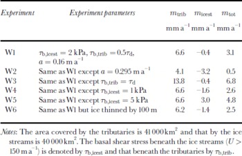
We computed melt rates using Equation (1) and the assumptions described above. The results for Ice Stream A/Whillans Ice Stream are summarized in Table 2, and the results for Ice Stream C are summarized in Table 3. In each case, we ran an initial experiment (W1, C1) based on our best estimate of the parameters needed to determine melt rate. There is a reasonable amount of uncertainty in these parameters, so we conducted several additional experiments (W2–W6, C2–C8) to examine the sensitivity of melt-rate estimates to the model parameters.
Model results for several experiments on Whillans Stream and Ice Stream A
Model results for several experiments on Ice Stream C

Our initial experiment (W1) for Ice Stream A and Whillans Ice Stream yielded a net melt rate of 3.1 mm a−1 with a 6.6 mm a−1 net melt rate for the tributaries and a net freeze-on rate of 0.4 mm a−1 for the ice streams. The spatial pattern of melt for this experiment is shown in Figure 2. Whillans B1 and B2 are estimated to have only slightly positive melt rates, while on much of the ice plain basal freeze-on is estimated to occur at rates of 0–2 mm a−1. There is a region near Crary Ice Rise with freeze-on rates of about 4–6 mm a−1. In experiment W2, we used a =0.295 ma−1, which yielded a net basal melt rate of 0.5 mm a−1. Experiments W3–W5 demonstrate the sensitivity of melt to basal shear stress. We note that the value of τb = 5 kPa in experiment W5 is unrealistically high for much of the ice plain since it exceeds the driving stress in some places. I n experiment W6 there was a decrease in total melt rate to 2.5 mm a−1 in response to a 100 m thinning of the ice sheet, with sufficient time to reach a new steady-state temperature profile.
We conducted a similar set of experiments for Ice Stream C (C1–C8). I n C1 we used ae ff = 0.295ma−1, which is the value derived from the borehole-temperature fits. With this value, the ice stream would have had an average melt rate of only 1.5 mm a−1 when it was active. Figure 2 indicates that the freeze-on rates on the active Ice Stream C likely ranged from about 2 to 8 mm a−1. I f instead we use the effective accumulation rate for Whillans Ice Stream (ae ff = 0.16ma−1), then the total average melt rate increases to 3.9 mma−1 in experiment W2. I n varying the basal shear stress (C3–C5) the range of average melt rates varies from 1.1 to 3.2 mm a−1. Thinning the ice stream by 100 m yields a net melt rate of 1.0 mm a−1. I n experiment C7, we reduced the velocity on the formerly active portion of Ice Stream C to close to its present-day value. This increased the basal freeze-on rate on the ice stream from 4.8 to 7.1 mm a−1. I n experiment C8, we increased the active ice-stream velocity estimate by 50%, which increased the total melt rate by 0.4 mm a−1.
In the above results, we have neglected basal melt beneath slow-moving ( 5 25 m a−1) areas of the inland catchment. To examine this contribution, we estimated basal melt in these regions. We first determined areas where melt should occur by solving for temperature, with the surface temperature and the basal temperature gradient (determined by G) specified as boundary conditions. Areas with temperature greater than or equal to Tpmp were assumed to be melting. For the regions where melt was found to be occurring, we used Equations (1) and (2) to determine the melt rate. In deriving these estimates, we assumed the motion in the slow areas was due entirely to internal deformation (e.g. no sliding) and that, consequently, there was no basal shear heating.
For the Ice Stream C catchment, we estimated a total melt of 0.038 km3 a−1, with an average melt rate 0.84 mm a−1 over an area of 45 000 km2 using a Giov. With aeff=0.295 m a−1, the average melt rate was 0.68 mm a−1 over an area of 7000 km2 for a total of 0.005 km3 a−1. These values represent approximate upper and lower bounds on inland catchment melt. Since most of this area corresponds to deep ice in the interior, the Byrd borehole suggests the actual value may be closer to the upper bound. For comparison, the tributary melt for experiment C1 was 0.22 km3 a−1, and the corresponding ice-stream freeze-on was 0.11 km3 a−1. Using a Giov the combined catchments of Ice Stream A and Whillans Ice Stream have an average inland melt rate of 0.61 mm a−1 for a total 0.015 km3 a−1 over an area of 24000 km2. For both catchments, the upper limit on melt generated beneath the slow-moving inland area was 520% of that generated beneath the tributaries.
Discussion
Even with considerable variation of the model parameters, our results indicate that, by and large, melting takes place beneath ice-stream tributaries, while low-melt or freeze-on conditions prevail beneath the active parts of Whillans Ice Stream and Ice Stream C. Unless we increase τb to unrealistically high levels, the model consistently predicts basal freezing beneath the thin ice of the ice plains. This indicates that, as suggested earlier by Reference RaymondRaymond (2000), import of basal melt from upstream appears to be a necessary condition to sustain motion on these ice streams. It is not a sufficient condition, however, since an appropriate drainage network is also required to redistribute the water from melting to freezing regions.
If ice-stream tributaries, by virtue of their higher basal shear stress and thicker ice, are the primary source of water that enables fast ice-stream flow, then this raises the issue of what length ice streams they could support. If grounding lines of Ice Stream C andWhillans Ice Stream were extended seaward by tens of km with similar thickness to their respective ice plains, then the area with net basal freeze-on would eventually out-compete the area with net basal melt. The distance from the meltwater source would also increase, placing additional constraints on the drainage network. Thus, it is likely that some additional basal melt source, beyond that of the present-day tributaries, is necessary to sustain very long, thin, well-lubricated paleo-ice streams. Multibeam sonar data indicate there were likely regions of exposed bedrock beneath portions of the Ross paleo-ice streams (Reference Anderson, Shipp, Alley and BindschadlerAnderson and Shipp, 2001), which perhaps could have provided basal shear heating to enable additional melt.
Flow speed onWhillans Ice Stream has decreased significantly over the last few decades (Reference Whillans, Bentley, van der Veen, Alley and BindschadlerWhillans and others, 2001; Reference Joughin, Tulaczyk, Bindschadler and PriceJoughin and others, 2002). Experiment W1suggests that presently there maybe sufficient melt to sustain motion, with possible additional meltwater from diversion of water from Ice Stream C (Reference Alley, Anandakrishnan, Bentley and LordAlley and others, 1994). The Unicorn temperature data, however, suggest that the temperature gradients for Whillans B1 and Ice Stream A may be closer to those of Ice Stream C than of Whillans B2. Experiment W2, which yielded less net melt than on Ice Stream C prior to stagnation, then may better represent conditions beneath the ice stream. If so, thenWhillans Ice Stream may well be headed toward complete stagnation within this century as the recent deceleration rates suggest. These results argue strongly in favour of additional drilling on the ice plain of Whillans Ice Stream to better constrain temperature estimates there.
The results for Ice Stream C yield average melt rates of ∼1.5mma–1. This means that the motion of the ice stream was particularly sensitive to piracy of basal meltwater (Reference Alley, Anandakrishnan, Bentley and LordAlley and others, 1994). In our experiments, we have assigned all the melt to Ice Stream C from the tributary that now appears to have been diverted to the catchment of Whillans B2 (see flow divides in Fig. 2). Diversion of the basal water flow from this tributary alone would likely have been sufficient to initiate stagnation. On the other hand, conditions may have been close enough to zero net melt (experiment C1) that stagnation could also have occurred without resorting to water piracy (Reference Price, Bindschadler, Hulbe and JoughinPrice and others, 2001; Reference Bougamont, Tulaczyk and JoughinBougamont and others, 2002).
Our experiments reveal a strong sensitivity to accumulation rate when only vertical advection and diffusion are considered in estimating melt rate. Furthermore, we used a steady-state solution in an area that is going through and has undergone significant change (Reference Conway, Hall, Denton, Gades and WaddingtonConway and other, 1999; Reference Fahnestock, Scambos, Bindschadler and KvaranFahnestock and others, 2000). Our attempts to use an effective accumulation rate correct some of the deficiencies in the model, resulting in better melt-rate estimates. This is clearly an artificial effect, however, that compensates for inadequacies in the model and does not suggest change in accumulation rate. While it appears that temperature estimates are improved, it is not very satisfying in that it does not explain the inadequacies of the model. We hypothesize that the model fails because tributary flow is strong enough to significantly depress basal melting through strong horizontal advection of ice from the interior. More detailed flowline and three-dimensional ice flow modeling, along with more borehole temperature data, are required to test this hypothesis.
Acknowledgements
I. Joughin performed his contribution to this work at the Jet Propulsion Laboratory, California Institute of Technology, under contract with National Aeronautics and Space Administration. S. Tulaczyk was funded by the U.S. National Science Foundation (NSF-OPP-0096302). The RADARSAT datawere acquired by the Canadian Space Agency and were downlinked and processed to L0-products by the Alaska SAR Facility. Mosaicked RADARSAT images and the surface digital elevation model (DEM) were provided by K. Jezek of the Byrd Polar Research Center. D. G.Vaughan and the BEDMAP project produced the bed-topography DEM. Many of the datasets we used were archived and distributed by the U.S. National Snow and Ice Data Center.



