





1. Introduction
Aeroacoustic liners are widely used passive noise control devices (Ma & Su Reference Ma and Su2020), typically consisting of perforated facesheets backed by cavities. Their performance is commonly described in the frequency domain by the acoustic impedance (Bauer Reference Bauer1977), a complex-valued quantity that defines a liner’s capacity to dissipate acoustic energy within a system.
Impedance is not a fixed property: it varies significantly with operating conditions, most notably under high sound pressure levels (SPLs) or when exposed to a shear grazing flow. In particular, vortex shedding at liner perforations, either acoustic or turbulent in origin, can generate locally nonlinear behaviours at SPLs far below those required for global nonlinear wave propagation (Ingard & Ising Reference Ingard and Ising1967; Melling Reference Melling1973; Tam et al. Reference Tam, Kurbatskii, Ahuja and Gaeta2001; Jing & Sun Reference Jing and Sun2002; Zhang & Bodony Reference Zhang and Bodony2012). The introduction of SPL-dependent nonlinearities complicates conventional measurement and optimisation approaches, as it requires accounting for a spatially varying impedance when the pressure field is non-uniform (Lafont et al. Reference Lafont, Méry, Roncen, Simon and Piot2020; Roncen et al. Reference Roncen, Méry, Piot and Klotz2022). Fundamentally, the emergence of a nonlinear term is associated with strong acoustic particle acceleration and large velocity gradients at the inlet and outlet of the perforated facesheet – typically of low porosity (porosity
 $\leq$
10 %) – as a direct consequence of mass-flow conservation.
The presence of a sheared mean flow can strongly influence the value of the impedance (Guess Reference Guess1975; Cummings Reference Cummings1986a ; Kirby & Cummings Reference Kirby and Cummings1998; Jones et al. Reference Jones, Watson and Nark2010), making its identification particularly challenging. Even a slight change in the displacement boundary-layer thickness can lead to widely different impedances (Quintino et al. Reference Quintino, Bonomo, Cordioli, Jones, Howerton, Nark and Avallone2025). It is also worth noting that the presence of flow modifies the optimal impedance of a system designed to maximise sound attenuation (Rice Reference Rice1969). Fundamentally, the interaction between the flow and the liner impedance remains poorly understood to date. It appears that the mean flow penetrates the perforated plate and alters the way the acoustic wave ‘sees’ the perforations. This phenomenon, commonly referred to as the vena contracta effect, reduces the effective cross-sectional area available for acoustic motion within the liner facesheet and therefore tends to increase the liner resistance, in a manner similar to that observed under steady bias flow (Jing & Sun Reference Jing and Sun1999). This behaviour bears strong resemblance to flow through porous media governed by Darcy–Forchheimer regimes, although this analogy is still rarely discussed in the acoustics literature (Shahzad et al. Reference Shahzad, Hickel and Modesti2022, Reference Shahzad, Hickel and Modesti2023; Hoang et al. Reference Hoang, Jafari, Cazzolato and Arjomandi2024), despite numerical results showing the difference between laminar and turbulent flow effects on an orifice impedance (Zhang & Bodony Reference Zhang and Bodony2016). In addition, the flow convects acoustically induced vortical structures (at high SPL), which may further alter the acoustic response of downstream perforations. For instance, recent studies by Paduano et al. (Reference Paduano, Scarano, Cordioli, Casalino and Avallone2026), carried out with a lattice Boltzmann method very large-eddy simulation (LBM–VLES), have evidenced that acoustic-induced velocity during the outflow phase generates a jetting-like mechanism at the orifice mouth, which displaces the near-wall fluid away from the wall and modifies the downstream boundary layer resulting in a different acoustic-induced velocity at the downstream cavities, which in turn might affect the dissipation mechanism (Howe Reference Howe1996; Scarano et al. Reference Scarano, Paduano and Avallone2025).
These external dependencies – high SPL and shear grazing flow – motivate continued efforts to reliably determine impedance in realistic flow and acoustic environments.
Direct measurement of impedance is generally not possible in the presence of flow, except with the intrusive and somewhat tricky in situ method (Dean Reference Dean1974; Bonomo et al. Reference Bonomo, Quintino, Spillere, Murray and Cordioli2024). Instead, researchers rely on indirect approaches known as impedance eduction. These methods combine experimental measurements – typically acoustic pressures or velocity fields in flow ducts – with wave propagation models, and determine the impedance that best reproduces the observed data (Watson et al. Reference Watson, Jones and Parrott1999; Jones et al. Reference Jones, Parrott and Watson2003; Jing et al. Reference Jing, Peng and Sun2008; Primus et al. Reference Primus, Piot and Simon2013; Spillere et al. Reference Spillere, Cordioli and Boden2017; Troian et al. Reference Troian, Dragna, Bailly and Galland2017; Weng et al. Reference Weng, Schulz, Ronneberger, Enghardt and Bake2018; Howerton et al. Reference Howerton, Vold and Jones2019; Qiu et al. Reference Qiu, Yang, Jing, Du and Sun2024). Most eduction techniques are rooted in the frequency domain, solving harmonic propagation problems given mean flow properties and an impedance boundary condition. Optimisation algorithms (Primus et al. Reference Primus, Piot and Simon2013; Watson & Jones Reference Watson and Jones2013) or Bayesian inference (Roncen et al. Reference Roncen, Mery, Piot and Simon2019) strategies are then employed to identify the impedance that either minimises the discrepancy or, equivalently, maximises the likelihood between experimental observations and model predictions. In the Bayesian framework, this procedure explicitly accounts for uncertainties in the model and measurements.
The pioneering observations of Renou & Aurégan (Reference Renou and Aurégan2011) revealed that, in the presence of flow, impedance inferred from upstream versus downstream wave propagation was not identical, challenging the long-held assumption that impedance is an intrinsic material property. This triggered a broad research effort into whether impedance alone suffices to capture the complex physics of liner–flow interactions. In particular, several studies investigated whether the mismatch could originate from limitations of the impedance boundary condition itself, leading to more sophisticated formulations accounting for finite boundary-layer thickness effects (Khamis & Brambley Reference Khamis and Brambley2016).
A key drawback of eduction strategies is that any deficiency in the propagation model or in the boundary-condition modelling is implicitly absorbed into the retrieved effective impedance. As a result, educed impedance can depend not only on the duct geometry or experimental method but also on the direction of acoustic waves relative to the mean flow, depending on the method used (Roncen et al. Reference Roncen, Piot, Méry, Simon, Jones and Nark2020). However, due to the tight coupling between the wave propagation modelling and the educed impedance, it has so far not been possible to sort out the upstream–downstream mismatch in terms of wave propagation modelling bias and genuine physical effects changing the impedance, such as the momentum transfer of Schulz et al. (Reference Schulz, Weng, Bake, Enghardt and Ronneberger2017). Weng et al. (Reference Weng, Schulz, Ronneberger, Enghardt and Bake2018) verified that the mismatch was not caused by neglecting viscosity in the wave propagation solvers used for eduction, while Roncen et al. (Reference Roncen, Méry, Piot and Klotz2022, § 3.2) showed that nonlinear effects on the liner can lead to a spatially varying impedance that differs depending on the excitation direction. Nevertheless, the upstream–downstream mismatch has also been observed in contexts where nonlinear liner effects can be neglected, indicating that the full picture remains unresolved. Furthermore, Roncen (Reference Roncen2025b ) suggested in a preliminary experiment that turbulence-induced noise may in part trigger the same nonlinearities as high SPL, further blurring the line between flow effects and acoustic response.
Taken together, these observations point towards two unresolved questions: the physical origin of the flow effect on liner impedance and the origin of the upstream–downstream impedance mismatch. The present work introduces a new time-domain methodology specifically designed to investigate these questions, the DIR-TDIBC (dynamic impulse response time-domain impedance boundary condition) framework (Roncen & Cardesa Reference Roncen and Cardesa2023). The DIR-TDIBC is based on instantaneous wall-normal velocity measurements, and, unlike conventional methods, reconstructs the liner impedance directly from the local velocity field without relying on a wave-propagation model. The method is assessed using both laser Doppler velocimetry (LDV) measurements and high-fidelity numerical simulations. Beyond its practical use as an impedance-evaluation tool, the method provides a means of isolating local liner–flow interactions from wave-propagation modelling effects, thereby providing a basis from which to revisit the two open questions identified above.
The paper is organised as follows. The theoretical background elements required for the modelling of the impedance of acoustic liners are introduced in § 2. The DIR-TDIBC approach is described in § 3. Experimental and numerical configurations are showcased in § 4. The method is applied to an LDV experiment conducted in an aeroacoustic bench in § 5, and to numerical data obtained via LBM–VLES in § 6. A discussion on the limits and merits of the method is given in § 7. Conclusions are drawn in § 8.
2. Theoretical background
This section introduces the theoretical background of liner impedance modelling, with a particular focus on frequency-domain quantities and models, as this constitutes a necessary step before transitioning to a time-domain approach. Section 2.1 presents the classical frequency-domain formulation of a single-degree-of-freedom (SDoF) liner, which serves as the reference liner material throughout this study, owing to its continued widespread use in the liner industry. Readers interested in more complex and efficient liners are referred to Jones et al. (Reference Jones, Simon and Roncen2022) for a review. Sections 2.3 and 2.4 then examine the influence of nonlinear and flow effects on impedance, respectively, and provide empirical model descriptions for both. Although only SPL-related nonlinear effects are incorporated into the time-domain approach proposed in this work, an empirical model describing flow effects is retained as a basis for comparison with previous studies.
2.1. Acoustic liner impedance
The normalised surface impedance, denoted by
 $Z$
in the frequency domain, is defined as the ratio of acoustic pressure
 $\tilde {p}$
to the normal acoustic particle velocity
 $\tilde {v}_{n}$
at the liner surface, scaled by the characteristic impedance of the ambient medium,
 $\rho _{\!f}c_{\!f}$
, where
 $\rho _{\!f}$
is the fluid density and
 $c_{\!f}$
the speed of sound. It is commonly expressed in terms of its real and imaginary parts – resistance
 $\tilde {r}$
and reactance
 $\tilde {\chi }$
– as
 \begin{equation} Z(\omega )=\frac {\tilde {p}(\omega )}{\rho _{\!f}c_{\!f}\tilde {v}_{n}(\omega )}=\tilde {r}(\omega )+\textit{j} \tilde {\chi }(\omega ), \end{equation}
where
 $\omega =2\pi f$
is the angular frequency in
 $\textrm {rad s}^{-1}$
, with
 $f$
the frequency in
 $\textrm {Hz}$
and
 $\textit{j}$
the imaginary unit.
It should be emphasised that
 $\tilde {p}$
and
 $\tilde {v}_{n}$
are typically interpreted as homogenised quantities, such that the fine-scale velocity variations within the perforations are not explicitly resolved. Instead, the liner surface is treated as acoustically smooth, and the impedance represents an effective boundary condition, that includes all the physical effects pertaining to the sound wave interaction, as shown in the graphical summary in figure 1 for a particular liner, the SDoF, as detailed in the sections below.
Graphical summary of the physical effects influencing the impedance. (a) Representation of an SDoF liner. (b) Representation of nonlinear and flow effects. (c) Representation of physical effects in play for the definition of the linear impedance. (d) A colour code is followed to associate each physics with the terms of the homogenised impedance in (2.2).

2.2. Linear impedance of an SDoF liner
Complex liners are often represented in the frequency domain as assemblies of elementary units using transfer matrix methods (Allard & Atalla Reference Allard and Atalla2009, Chap. 11). For clarity, however, a more compact SDoF formulation is adopted in this work, where only one perforated plate and one cavity are considered. The normalised impedance of an SDoF liner is expressed following the approach of Atalla & Sgard (Reference Atalla and Sgard2007, (8)), with the cavity wavenumber
 $\tilde {k}_{c}$
determined using the formulation of Bruneau (Reference Bruneau2006, § 3.7):
 \begin{align} Z_{0}\left (\omega \right ) = & \frac {R_{s}}{\rho _{\!f}c_{\!f}\phi _{p}} \left (\frac {2L_{p}}{r_{p}}+4\frac {\epsilon _{e}}{r_{p}}\right ) \frac {\left (1+\textit{j}\right )\sqrt {2}}{2} \notag \\[3pt] &+\frac {\left (2\epsilon _{e}+L_{p}\right )}{c_{\!f}\phi _{p}}\textit{j}\omega +\frac {1}{\phi _{c}}\mathrm{coth}\big (\textit{j}\tilde {k}_{c}H_{c}\big), \\[-12pt]\nonumber \end{align}
 \begin{align} \epsilon _{e} & = 0.85r_{p}\left (1-1.14\sqrt {\phi _{p}}\right ), \quad \text{correction length}, \\[-12pt]\nonumber \end{align}
 \begin{align} R_{s} &= \sqrt {\eta \omega \rho _{\!f}}, \quad \text{surface resistance}, \\[-12pt]\nonumber \end{align}
 \begin{align} \textit{j}\tilde {k}_{c} & = \frac {\textit{j}\omega }{c_{\!f}}\left [\frac {1+\left (\gamma -1\right )\varPhi \left (k_{\kappa }r_{c}\right )}{1-\varPhi \left (k_{\nu }r_{c}\right )}\right ]^{1/2}, \quad \text{cavity wavenumber}, \\[-12pt]\nonumber \end{align}
 \begin{align} \varPhi \left (s\right ) & = \frac {2}{s}\frac {I_{1}}{I_{2}}\left (s\right ). \end{align}
Here, an
 ${\rm e}^{+\textit{j}\omega t}$
convention is assumed, and the formulation is valid for
 $\omega \gt 0$
. The symbols
 $L_{p}$
,
 $\phi _{p}$
and
 $r_{p}$
denote, respectively, the thickness, porosity and hole radius of the perforated plate, while
 $H_{c}$
,
 $\phi _{c}$
and
 $r_{c}$
describe the cavity’s height, porosity and hydraulic radius. Here
 $I_{n}$
are modified Bessel functions of the first kind of order
 $n$
, with
 $k_{\nu }=\sqrt {\textit{j}\omega /\nu }$
and
 $k_{\kappa }=\sqrt {\textit{j}\omega /\kappa }$
. The ambient fluid is characterised by the speed of sound
 $c_{\!f}$
, density
 $\rho _{\!f}$
, heat capacity ratio
 $\gamma$
, dynamic viscosity
 $\eta$
, kinematic viscosity
 $\nu$
and thermal conductivity
 $\kappa$
.
2.3. Nonlinear effects
Although impedance is formally a concept tied to linear systems, in practice it is often extended to describe nonlinear behaviour in the frequency domain when harmonic excitation is considered. While this extension is not strictly rigorous, it has proven effective for characterising liner performance at high SPL (Billard et al. Reference Billard, Gabard, Versaevel and Tissot2020).
Most nonlinear impedance models (Ingard & Ising Reference Ingard and Ising1967; Melling Reference Melling1973; Guess Reference Guess1975; Cummings Reference Cummings1986b ; Temiz et al. Reference Temiz, Tournadre, Arteaga and Hirschberg2016; Boden et al. Reference Boden, Shah and Boij2024) adopt an additive formulation in which the total impedance is expressed as
 \begin{equation} Z_{\textit{tot}}\left (\omega ,\tilde {v}_{n}\left (\omega \right )\right )=Z_{0}\left (\omega \right )+\mathcal{G}_{\textit{NL}}\left (\omega ,\,\tilde {v}_{n}\left (\omega \right )\right ), \end{equation}
where
 ${{Z}}_{0}(\omega )$
is the baseline linear impedance and
 $\mathcal{G}_{\textit{NL}}$
is a nonlinear contribution that depends on frequency, perforation geometry, plate porosity and the normal particle velocity
 $\tilde {v}_{n}(\omega )$
at the liner surface. Depending on the author, the particle velocity may be defined in different ways, based either on the root-mean-square (r.m.s.) value of the particle velocity over time or on its peak magnitude. In order to apply the time-domain methodology presented in this work, an r.m.s.-based formulation must be adopted.
In this study, the nonlinear correction
 $\mathcal{G}_{\textit{NL}}$
is split into real and imaginary parts using empirical models recommended by Boden et al. (Reference Boden, Shah and Boij2024). The real component is estimated using the formulation of Temiz et al. (Reference Temiz, Tournadre, Arteaga and Hirschberg2016, (13)), while the imaginary part is modelled with the correction of Shah et al. (Reference Shah, Bodén and Boij2024, (14)). For reference, these empirical models are provided here for
 $\omega \gt 0$
:
 \begin{equation} \textrm {Re}\left (\mathcal{G}_{\textit{NL}}\right ) =\frac {\sqrt {2}\left |\tilde {v}_{n}\right |}{\phi _{p}^2c_{\!f}}\frac {1}{2C_{\textit{vc}}^2}\frac {1}{1+2{S_t}\left (1+0.06\text{e}^{ {3.74}/{{S_h}}}\right )} \end{equation}
and
 \begin{equation} \textrm {Im}\left (\mathcal{G}_{\textit{NL}}\right )=\frac {k_{\!f}r_{p}}{\phi _{p}}\left [-\big(0.6+1.6{S_h}^{-1}+0.015{S_h}\big )\left (1-\frac {1}{1+0.013{S_t}^{-2.5}{S_h}^{2}}\right )\right ]\!, \end{equation}
where
 $k_f=\omega / c_f$
is the air wavenumber,
 $C_{\textit{vc}}=0.8$
is the vena contracta coefficient,
 $S_h$
is the shear wavenumber and
 $S_t$
is the Strouhal number based on the r.m.s. particle velocity inside the perforation
 $\tilde {u}_{p} (\omega )=\left |\tilde {v}_{n} (\omega )\right |/\phi _{p}$
:
 \begin{equation} {S_h} =r_{p}\sqrt {\frac {\omega }{\nu }}, \end{equation}
 \begin{equation} {S_t} =\frac {2\omega r_{p}}{\sqrt {2}\tilde {u}_{p}\left (\omega \right )}. \end{equation}
The real part of the proposed nonlinear model is quite sensitive to the choice of the vena contracta coefficient
 $C_{\textit{vc}}$
. In the present work, a value of
 $C_{\textit{vc}}=0.8$
was selected, slightly higher than the typical value reported for sharp-edged orifices (
 $C_{\textit{vc}}\approx 0.75$
), in order to account for the bevelling of the perforations in the liner samples considered in the present work (Moers et al. Reference Moers, Hirschberg, Tonon, Lopez and Smeulders2011, Chap. 4).
2.4. Flow effects
Typically, in the presence of a shear grazing flow, an additional contribution to the impedance is added, as
 \begin{equation} Z_{\textit{tot}}\left (\omega ,\tilde {v}_{n}\left (\omega \right )\right )\xleftarrow {}Z_{\textit{tot}}\left (\omega ,\tilde {v}_{n}\left (\omega \right )\right )+\mathcal{G}_{\textit{flow}}\left (\boldsymbol{U}_{\boldsymbol{0}}\right ), \end{equation}
where
 $\mathcal{G}_{\textit{flow}} (\boldsymbol{U}_{\boldsymbol{0}} )$
is usually a real function of the liner’s flow-facing porosity and of the flow profile
 $\boldsymbol{U}_{\boldsymbol{0}}$
(Guess Reference Guess1975; Yu et al. Reference Yu, Ruiz and Kwan2008).
A common simplification is to consider the Goodrich model of Yu et al. (Reference Yu, Ruiz and Kwan2008) for a liner placed in a flow duct, as
 \begin{equation} \mathcal{G}_{\textit{flow}}\left (\boldsymbol{U}_{\boldsymbol{0}}\right ) = \frac {M_{\textit{b}}}{\phi _p \left (2+1.256\frac {\delta ^\star }{d} \right )} M_{\textit{b}}, \end{equation}
where
 $M_{\textit{b}}$
is the bulk Mach number and
 $\delta ^\star$
is the boundary-layer displacement thickness. Parameter
 $\delta ^\star$
is defined as
 \begin{equation} \delta ^\star = \int _{0}^{H/2} \left(1-\frac {U(y)}{U_0}\right) \text{d}y, \end{equation}
where H is the height of the duct.
In the remainder of this work, impedance evaluation within the time-domain framework does not incorporate explicit flow corrections through the Goodrich model or related formulations of (2.6). Instead, only the linear and nonlinear contributions of (2.3) are retained. The wall-normal component of the turbulence-induced velocity field is assumed to affect the effective impedance exclusively through the nonlinear mechanisms described by (2.4).
This approach constitutes a significant departure from classical studies, in which flow effects are typically represented through non-local static quantities such as the Mach number. Here, following the initial exploration of Roncen (Reference Roncen2025b , § 5), we hypothesise that the empirical correlations proposed in earlier works are, at least in part, directly driven by wall-normal velocity fluctuations induced by turbulence. In this view, these fluctuations modulate the impedance in a manner analogous to acoustic velocity fluctuations.
To test this hypothesis, the wall-normal velocity fields measured experimentally or obtained numerically above a liner – encompassing both hydrodynamic and acoustic perturbations – are injected into a time-domain representation of the nonlinear impedance.
If the hypothesis holds, the resulting impedance should coincide with that predicted by classical empirical models based on Mach number scaling, such as the Goodrich model, which is used here solely for comparison owing to its simplicity and widespread adoption.
2.5. The reflection coefficient
The numerical method employed throughout this work is formulated in terms of the liner’s reflection coefficient. The reflection coefficient, sometimes referred to as the scattering operator
 $R$
, is bounded within the complex unit circle, which makes it particularly convenient and numerically stable for simulation purposes (Delorme et al. Reference Delorme, Mazet, Peyret and Ventribout2005, § 3.3; Ventribout Reference Ventribout2006, § 2.3; Monteghetti Reference Monteghetti2018, § 5.3). Moreover,
 $R$
is bijectively related to the normalised impedance through the relation
 \begin{equation} R\left (\omega ,\tilde {v}_{n}\left (\omega \right )\right )=\frac {Z_{\textit{tot}}\left (\omega ,\tilde {v}_{n}\left (\omega \right )\right )-1}{Z_{\textit{tot}}\left (\omega ,\tilde {v}_{n}\left (\omega \right )\right )+1}. \end{equation}
In practice, however, results are reported in terms of impedance, as this representation is the most commonly used and readily interpreted within the liner community.
3. The DIR-TDIBC methodology
This section is dedicated to the new methodology developed in this work, and on how it can be applied to practical cases of interest. Section 3.1 addresses the conversion from frequency to time domain, as done by the DIR-TDIBC method. Section 3.2 presents how the method is applied in a context where hydrodynamic and acoustic perturbations coexist, as well as the associated hypotheses that were made. The post-treatment of time-domain signals into the frequency domain is discussed in § 3.3. A schematic summarising the DIR-TDIBC method is shown in figure 2.
Graphical summary of the DIR-TDIBC method applied in a nonlinear context, where the normal velocity – measured by LDV or via probes in high-fidelity simulation – is used to replay the nonlinear behaviour during the convolution of (3.2).

3.1. The dynamic impulse response approach to TDIBC
In this work, the liner’s impulse response – defined as the inverse Fourier transform of its response to a unit impulse – is used as the fundamental building block. In discrete form, the reflection coefficient can thus be represented as a finite-length impulse response array
 $\mathcal{R}$
, evaluated as
 \begin{equation} \mathcal{R}\left ( t, v_n \left ( t \right ) \right )=\mathcal{F}^{-1} \{ R\left (\omega ,v_n \left ( t \right )\right ) \}, \end{equation}
where
 $\mathcal{F}^{-1}$
is the inverse Fourier transform operator and where
 $v_n$
is the instantaneous wall-normal velocity above the liner (represented by the red curve in figure 2). Consequently, the impulse response evolves continuously with the instantaneous value of
 $v_n$
, and each spatial location on the liner is associated with its own time-varying impulse response.
This choice leverages the flexibility of the impulse response: any time-domain signal can be represented as a sequence of instantaneous values, so knowing the liner’s response to a unit impulse allows its response to arbitrary inputs to be predicted by summing the contributions of each discrete pulse.
Strictly speaking, the impulse response is not uniquely defined for a nonlinear system. In the present work, it is recalculated at each time step to account for the instantaneous velocity at the perforation, which is assumed sufficient to capture the system’s nonlinearity. Conceptual limitations of this approach were discussed by Roncen (Reference Roncen2025b , § 3.3.1).
In numerical solvers, impulse responses can be efficiently accumulated using arrays: a reference array stores the precomputed response, which is then sequentially processed into a secondary array to accumulate the boundary condition’s future response. This DIR-TDIBC approach, first proposed by Roncen & Cardesa (Reference Roncen and Cardesa2023), extends naturally to nonlinear operators and can handle both harmonic and broadband signals, including those with discontinuities.
The time-local dynamic convolution between an incident wave
 $x(t)$
and the reflection coefficient is expressed as
 \begin{equation} y(t_K) = \sum _{k=0}^{K} x(t_k)\, \mathcal{R}\bigl (t_K - t_k,\, v_{n,k}\bigr ), \end{equation}
where
 $x(t)$
denotes the incident wave amplitude,
 $y(t)$
the reflected wave amplitude,
 $\mathcal{R}$
the (generally nonlinear) impulse response kernel and
 $v_{n,k}$
the instantaneous wall-normal velocity at time
 $t_k$
.
Using the instantaneous velocity rather than its r.m.s. value provides superior temporal resolution for modelling complex, time-varying excitations, as demonstrated by Roncen (Reference Roncen2025b
). In the present framework, the incident amplitude
 $x(t)$
is prescribed by the user, typically as a sinusoidal signal at the acoustic excitation frequency (see the blue signal in figure 2).
This differs from the approach of Roncen (Reference Roncen2025b
), in which the incident amplitude was obtained through a wave-sorting procedure and subsequently combined with the reflected wave to evaluate
 $v_{n,k}$
. Here, the particle velocity governing the nonlinear behaviour of the impulse response is not derived from
 $x(t)$
and
 $y(t)$
; instead, it is directly extracted from velocity measurements and imposed as an external input to the time-domain model, as represented by the red dashed arrow connecting the total normal velocity to the convolution evaluation in figure 2.
At each simulation step
 $t_k$
, the impulse response is obtained via the inverse Fourier transform of
 $R$
, using the instantaneous velocity in place of the frequency-domain velocity in (2.3) and (2.9):
 \begin{equation} \mathcal{R}\left (t, v_{n,k}\right ) = \frac {1}{2\pi } \int _0^{\infty } R \left (\textit{j} \omega , |v_{n,k}| \right ) {\rm e}^{\textit{j} \omega t} \, \textrm {d}\omega . \end{equation}
Precomputing responses for representative values of the total wall-normal velocity
 $v_i$
(see figure 2) and interpolating between them avoids recalculation at each time step, enabling efficient and accurate simulations.
In practice, 200 discrete values of
 $v_i$
were used, uniformly distributed between the minimum and maximum of
 $|v_n|$
observed in the signal. For each value, a corresponding impulse response was precomputed, forming a lookup table used during the time-domain convolution. At each time step, the appropriate response is obtained via linear interpolation in
 $v_i$
. The accuracy of this interpolation strategy was independently verified by comparison with direct (non-interpolated) evaluations on selected test cases, showing negligible deviation.
For experimental validation of this approach under nonlinear conditions with single-tone and multi-tone excitations, see e.g. Roncen & Cardesa (Reference Roncen and Cardesa2023) and Roncen (Reference Roncen2025b ). Numerical implementation details, including nonlinear cases, are provided in shared Python codes (Roncen Reference Roncen2025a ).
Alternative methods, such as Diab’s model (Diab et al. Reference Diab, Dragna, Salze and Galland2022) updated for instantaneous velocity, Moufid’s volume-based approach (Moufid et al. Reference Moufid, Roncen, Matignon and Piot2024) or Monteghetti’s nonlinear oscillo-diffusive method (Monteghetti et al. Reference Monteghetti, Matignon and Piot2018), could yield comparable or better results. The DIR-TDIBC is chosen here primarily for its simplicity of implementation.
3.2. Acoustics, turbulence and the DIR-TDIBC
The goal of the DIR-TDIBC method is to produce, from an incident acoustic wave, a reflected wave that will encompass the full acoustic behaviour of the aeroacoustic liner, including its nonlinear effects and its flow effects. A fundamental limitation of the approach, however, is that the incident wave at the liner surface is not directly accessible. Instead, only the wall-normal velocity measured above the liner is available.
In experiments, the wall-normal velocity can be measured using LDV or time-resolved particle image velocimetry. Similarly, in high-fidelity numerical simulations – where the liner is resolved down to each perforation and no impedance boundary condition is imposed – the velocity can also be extracted directly. In both cases, the concept of homogenised impedance becomes critical: if measurements are taken too close to the liner, the notion of impedance loses its physical meaning. This issue will be further addressed in the discussion of the results.
Whether obtained from experiments or high-fidelity simulations, the evaluated wall-normal velocity signal in the time domain
 $v_n (t )$
contains multiple contributions: the mean flow
 $v_0$
, hydrodynamic fluctuations related to turbulence
 ${v}_{\textit{hyd}} (t )$
and acoustic-induced perturbations
 $v_{\textit{ac}} (t )$
:
 \begin{equation} v_n\left (t\right ) = v_0 + {v}_{\textit{hyd}}\left (t\right ) + v_{\textit{ac}}\left (t\right ), \end{equation}
where we define the fluctuating velocity as
 \begin{equation} v^\prime = {v}_{\textit{hyd}}\left (t\right ) + v_{\textit{ac}}\left (t\right ). \end{equation}
In the remainder of this work, we also define the mean-removed r.m.s. fluctuating velocity
 $v^\prime _{\textit{rms}}$
as
 \begin{equation} v^\prime _{\textit{rms}} = \sqrt {\frac {1}{N_t}\displaystyle \sum _{i=1}^{N_t} {v^\prime }\left (t_i\right )^2}, \end{equation}
with
 $N_t$
the number of samples in the time-domain signal.
In the present work, two strong modelling assumptions are introduced, in order to consider a one-way coupling between turbulence and acoustics:
-
(i) Hypothesis 1: The impedance characterises exclusively the transfer function between acoustic quantities, and turbulent contributions are not directly modulated by the impedance. In other words, the divergence-free component of the velocity field – associated with hydrodynamic fluctuations – is assumed to be unaffected by the impedance, whereas the irrotational component – associated with acoustically induced fluctuations – is governed by it.
-
(ii) Hypothesis 2: Turbulence-induced velocity fluctuations contribute to the onset of nonlinear effects described by (2.4a )–(2.4b ). This contribution is accounted for directly in the time domain by updating the impulse response in (3.1) at each time step, using the total wall-normal velocity
 $v_n(t)$
, obtained either experimentally from LDV measurements or numerically from probe data.

Once the total normal velocity above the liner is known, the impedance nonlinear behaviour is therefore fully prescribed in time. An incident wave must then be supplied to the DIR-TDIBC convolution – this corresponds to
 $x(t)$
in (3.2). In a Navier–Stokes characteristic boundary condition framework,
 $x(t)=p_{\textit{ac}}(t)/(\rho _{\!f}c_{\!f})-v_{\textit{ac}}(t)$
corresponds to the incoming acoustic characteristic. During this convolution, the nonlinear response is numerically reconstructed by injecting
 $v_n(t)$
in place of
 $\tilde {v}_n$
in (3.1), with the impulse response updated at every time step in (3.2).
The normal velocity
 $v_n (t )$
is assumed to be representative of the velocity experienced by a homogeneous impedance boundary condition. This assumption breaks down in the immediate vicinity of the liner, where the impedance is discontinuous due to perforation–rigid wall interfaces. Nevertheless, it is assumed that at a sufficient distance above the liner, a homogenised velocity field can be recovered, and that the measured velocity provides a meaningful estimate of the response that would be obtained in an idealised homogeneous configuration.
The above procedure is repeated for each velocity measurement performed above the liner, within a certain distance. This yields the spatial evolution of the impedance as a function of the frequency, over an extended frequency band.
We reiterate that the requirement to use this method is quite strong in terms of modelling, as one already needs to know, through a model such as (2.3), the proper behaviour of the liner in a linear or nonlinear context. Consequently, the method should be viewed primarily as a tool for assessing the relative effect of flow noise on a liner’s impedance. Nevertheless, provided that the frequency-domain models employed are accurate, which is expected for well-studied liners such as SDoF liners, the resulting impedance estimates are expected to be close to the true values.
3.3. Signal processing procedure
The velocity signals obtained from the LDV measurements and the LBM–VLES simulations were processed using similar workflows, with a few case-specific differences. The LDV post-processing is described first, followed by the modifications applied to the LBM–VLES data.
For each measurement location, the wall-normal velocity signal was interpolated onto a uniformly sampled time grid using linear interpolation over the
 $\approx 10\mathrm{\ s}$
of acquisition. The resulting signal was divided into overlapping segments of 1 s in duration (approximately 1400 acoustic periods), with a 50 % overlap between consecutive segments.
Each segment was supplied to the DIR-TDIBC framework, and the reflected acoustic wave was reconstructed through the dynamic convolution procedure described in § 3.1. The resulting time-domain signal was multiplied by a Hanning window prior to Fourier transformation. The reflection coefficient was then extracted at the acoustic excitation frequency and converted into impedance using (2.9).
For the LES, only a single 11.4 ms realisation (16 acoustic periods) was available due to the computational cost of the high-fidelity simulation. No temporal interpolation was required since the time step was fixed.
4. Experimental and numerical configurations
The methodology developed in this work is applied to two distinct datasets:
-
(i) experimental measurements performed in the ONERA B2A wind tunnel using LDV velocity measurements above an acoustic liner (ONERA sample), whose analysis is detailed in § 5, and
-
(ii) high-fidelity numerical simulations of turbulent flow over a perforated liner using an LBM–VLES approach carried out at PoliTo (PoliTo sample), whose analysis is detailed in § 6.
Although both configurations involve grazing flow over an SDoF liner and are analysed using the same impedance-eduction methodology, they were originally developed in separate studies and were not designed as a strict one-to-one comparison case.
Nevertheless, the two configurations share many important features. In both cases, the liner consists of a perforated facesheet covering an array of square cavities, and the acoustic response of the liner is investigated under turbulent-grazing-flow conditions with a harmonic acoustic excitation. The flow Mach numbers, excitation frequencies and general geometric scales are also comparable. This similarity makes it possible to apply the same analysis framework to both datasets and to examine how the proposed methodology behaves in two complementary contexts: a controlled experimental environment and a fully resolved numerical dataset where the reference impedance can be directly evaluated.
At the same time, several differences must be emphasised. The experimental configuration corresponds to the B2A facility geometry and liner sample, whereas the numerical simulation reproduces a liner test rig geometry inspired by the UFSC facility (Quintino et al. Reference Quintino, Bonomo, Cordioli, Jones, Howerton, Nark and Avallone2025). As a result, some geometric parameters differ, including perforation diameter and global porosity. The acoustic excitation frequency and the accessible measurement locations are also not identical. In addition, the numerical simulation employs a reduced spanwise domain with periodic boundary conditions, which constrains the development of large turbulent structures compared with the experimental facility. Additional information on the measurement methodology, velocity field and spectral content is provided by Ambrosiani et al. (Reference Ambrosiani, Piot, Mery and Avallone2026). The reliability of the numerical results is supported by a dedicated mesh-convergence analysis and comparison with experiments reported by Paduano et al. (Reference Paduano, Scarano, Cordioli, Casalino and Avallone2026), while a more comprehensive characterisation of the velocity field and its energy content is provided by Scarano et al. (Reference Scarano, Lyu, Paduano and Avallone2026).
Consequently, the purpose of presenting both datasets is not to perform a direct quantitative validation of the numerical simulation against the experiment. Instead, they should be viewed as two representative configurations that allow the proposed methodology to be evaluated under realistic conditions. The experimental dataset provides insight into the behaviour of the method with real measurements affected by noise, limited spatial resolution and experimental uncertainties. The numerical dataset, on the other hand, offers a controlled environment in which the true impedance can be determined independently, enabling a more direct assessment of the method’s accuracy.
The main characteristics of the experimental and numerical configurations are summarised in table 1, which highlights both their similarities and their differences. The predicted linear impedance of each sample, obtained from (2.2), is shown in figure 3. The flow profiles measured without acoustic excitation just upstream and downstream of the liner samples are shown in figure 4. The following sections then describe the experimental set-up and the numerical methodology in detail before presenting the corresponding results.
Main characteristics of the experimental and numerical configurations analysed in this study.

Table 1. Long description
A table comparing the main characteristics of experimental and numerical configurations. The table has 18 rows and 3 columns. Column headers are Parameter, Experiment, and Numerical simulation. Row labels include Liner name, Configuration origin, Duct cross-section, Liner type, Liner length, Cavity depth, Cavity side length, Cell pitch, Cavity wall half-thickness, Facesheet thickness, Orifice diameter, Number of orifices per cavity, Orifice spacing, Orifice shape, Global porosity, Local porosity, Flow Mach number, Liner resonance frequency, Acoustic excitation frequency, Acoustic excitation level, Measurement zones, Measured quantity, Reference impedance availability. Values are provided for each parameter under the Experiment and Numerical simulation columns.
Predicted linear impedance of the ONERA and PoliTo samples. (a) Resistance. (b) Reactance.

Comparison of flow profiles in the B2A duct (obtained via LDV) and in the LES carried out at PoliTo, evaluated in all cases at the same spanwise location. In the LDV case, the measurements are taken 3 mm away from the liner, while in the LES case, the evaluation is exactly at the liner beginning and end. The experimental profiles are extended to
 $y = 0$
by imposing the wall boundary condition
 $U_0(0) = 0$
, although the LDV measurements are available only for
 $y/H \gtrsim 0.04$
.

5. Application of DIR-TDIBC to LDV measurements
This section introduces the experimental set-up used at ONERA for the liner characterisation under shear-grazing-flow conditions. Section 5.1 presents the B2A wind tunnel facility, § 5.2 the LDV set-up and § 5.3 the liner sample used in this work. The configurations under study are detailed in § 5.4, and results of the DIR-TDIBC analyses are presented in § 5.5.
5.1. The B2A wind tunnel
The ONERA B2A facility consists of a 4 m long stainless-steel duct with a square cross-section of
 $50\,{\rm mm} \times 50$
mm. The
 $0.2$
m long test section is equipped with silica windows for optical access, and the duct termination features a quasi-anechoic outlet, yielding a downstream reflection coefficient below
 $0.2$
for frequencies above 500 Hz. The facility, shown in figure 5, can generate fully developed turbulent flows with bulk Mach numbers up to
 $M_{\textit{b}} = 0.6$
, where the turbulence intensity in the test-section centreline is of the order of a few per cent. Two acoustic drivers located upstream or downstream of the test section can produce multi-tone signals of up to 150 dB over the frequency range 300–3500 Hz. The test liner occupies a
 $150$
mm long segment of the lower duct wall. Six microphone locations are available on the upper wall to measure the acoustic pressure field upstream of the liner leading edge and downstream of the liner trailing edge. The upper wall facing the liner is equipped with 16 microphone locations ranging from
 $x = -27 \mathrm{\ mm}$
to
 $x = 177 \mathrm{\ mm}$
from the liner origin with a step of
 $12\mathrm{\ mm}$
between each location as represented in figure 6. Two flush-mounted GRAS microphonic probes are used (probe diameter of 1.2 mm) to set the incident upstream or downstream acoustic excitation and to measure the SPL at the wall opposite the liner via a wave-sorting procedure (Lafont et al. Reference Lafont, Méry, Roncen, Simon and Piot2020). A single microphone is then used at each measurement location to retrieve the pressure signal, without phase mismatch between measurements.
The B2A facility located at ONERA Toulouse.

5.2. The LDV set-up
A two-component fringe-mode LDV system enables measurement of both axial and vertical velocity components across nearly the entire volume of the test section, using a displacement bench. This measurement system was composed of a laser emitting green (514.5 nm) and blue (488 nm) wavelengths. The two pairs of beams were issued by a DANTEC 55X emitting head equipped with a 240 mm focal lens. The fringe spacing for the green beam is
 $2.23\,{\unicode[Arial]{x03BC}} \mathrm{m}$
and the fringe spacing for the blue beam is
 $2.15\,{\unicode[Arial]{x03BC}} \mathrm{m}$
. The crossing angles are measured and used as an input for the post-processing of the signals. The transformation matrix has an accuracy estimated to be lower than 1 %. Signals were processed by a DANTEC BSA burst spectrum analyser. The emitting optics produce an elliptical measurement volume whose minor axis can be as small as 70 μm and the major axis is about 0.7 mm.
Flow is seeded with amorphous silica particles, chosen for their low tendency to deposit on optical windows. Because particles arrive randomly in the measurement volume, the LDV signal is unevenly sampled; a reconstruction algorithm is used to resample the raw data at a uniform rate by the use of a linear interpolation in time. Each velocity component is measured at a minimum rate of
 $f_m \approx 15\,000$
samples per second with a
 $97\,\,\%$
validation rate in coincidence, with more than 250 000 total samples acquired at each measurement location.
The experiments were conducted under standard atmospheric conditions, with the flow temperature maintained at ambient
 $T_0 \approx 20\,^\circ \mathrm{C}$
, with maximum fluctuations of
 $1\,^\circ \mathrm{C}$
, corresponding to a sound speed of
 $c_0 \approx 343\,\mathrm{m\,s}^{-1}$
. The mass flow rate was maintained constant at either 100 or 300 g s−1 for all experiments, corresponding to a bulk Mach number of either
 $M_{\textit{b}} = 0.1$
or
 $M_{\textit{b}} = 0.3$
.
The resulting LDV dataset comprises over 120 spatial measurement points per tested configuration. The system provides two-dimensional velocity fields in the
 $x$
line at
 $y=1\, \mathrm{mm}$
or
 $y=2.5\, \mathrm{mm}$
from the liner surface and
 $z=6.34\,\mathrm{ mm}$
away from the centre of the sample, centred in the middle of a row of cavities, as shown by the green dashed line in figures 6 and 7. Only the streamwise and vertical (normal to the liner) components are measured.
Schematics of the LDV measurement and microphone locations. Upstream and downstream excitations are never on simultaneously. The green line represents the spanwise location of LDV measurements and can be located at different heights above the liner sample.

5.3. Liner sample
The acoustic liner used for this study is an SDoF liner made of a perforated plate over squared cavities based on a geometry shared between multiple facilities (Quintino et al. Reference Quintino, Bonomo, Cordioli, Jones, Howerton, Nark and Avallone2025). Each cavity is covered by a thin plate of
 $0.635\,\mathrm{mm}$
with eight orifices of diameter
 $d = 0.991\,\mathrm{mm}$
for a total porosity of
 $\phi _p = 3.95\,\%$
. The cavity height is
 $H_c = 38.1 \,\mathrm{mm}$
, with a side length of
 $D = 9.91\,\mathrm{mm}$
. A top-view sketch is given in figure 7, with the LDV line superimposed to give its location over the liner.
Top-view sketch of the liner SDoF sample. The green line represents the spanwise position of the LDV measurement line and is located at different heights above the liner sample. Length
 $L_c=12.44$
mm represents the inter-cell distance.

Before presenting the results, a particular feature of the tested liner sample must be discussed. The sample is composed of
 $N$
elementary cells, separated by thick walls – whose half-thickness
 $w_p$
is given in table 1 – which account for approximately
 $37\,\%$
of the liner surface area, as represented in figure 8. Using the notations in the figure,
 $\varSigma _2/\varSigma _1=0.63$
. When considering the cell as a whole (
 $\varSigma _1$
), the global porosity is
 $3.95\,\%$
. However, if one examines only the perforated regions of each acoustically active cell, excluding the cavity walls, the effective (local) porosity based on
 $\varSigma _2$
rises to
 $6.5\,\%$
.
Top-view and side-view perspective of a liner cell.

To correctly represent the impedance under this interpretation, the liner can be modelled as a dual liner composed of two distinct cell types assembled in parallel: rigid walls in
 $\varSigma _1 \setminus \varSigma _2$
and SDoF resonators with a porosity of
 $6.5\,\%$
in
 $\varSigma _2$
. This modelling choice has implications for the predicted nonlinear behaviour of the liner, since nonlinear effects are directly influenced by the local porosity; see (2.4a
) and (2.4b
). Overall, our choice seems to be aligned with the recent conclusions of Jones & Nark (Reference Jones and Nark2023).
5.4. Configurations under study
Measurements were performed during an LDV experiment at bulk Mach numbers of
 $0.1$
and
 $0.3$
, with an acoustic excitation at 1500 Hz ranging from 115 to 145 dB (incident SPL at the entrance of the test section). The experiment was performed with both loudspeakers being either upstream or downstream of the liner section. The methodology described in § 3.2 is performed on each of the
 $\approx 120$
LDV measurement points located on a line 1 mm above the liner (see figure 6).
Table 2 summarises the configurations under study.
Experimental configurations studied by LDV in the B2A facility.

Table 2. Long description
A table summarizing experimental configurations studied by LDV in the B2A facility. The table has five rows and four columns. The columns are labeled Experimental configuration, Mach, SPL (incident) (dB), and Loudspeaker position. Row 1: Experimental configuration 1, Mach 0.1, SPL (incident) (dB) 115, Loudspeaker position Upstream. Row 2: Experimental configuration 2, Mach 0.1, SPL (incident) (dB) 130, Loudspeaker position Upstream. Row 3: Experimental configuration 3, Mach 0.1, SPL (incident) (dB) 145, Loudspeaker position Upstream. Row 4: Experimental configuration 4, Mach 0.3, SPL (incident) (dB) 145, Loudspeaker position Upstream. Row 5: Experimental configuration 5, Mach 0.3, SPL (incident) (dB) 145, Loudspeaker position Downstream.
(a) Mean and (b) mean-removed r.m.s. components of the wall-normal velocity field above the liner at a distance of 1 mm. Length
 $L_c$
denotes the inter-cell distance, as represented in figure 7.

5.5. Results
We first characterise in § 5.5.1 the combined flow and acoustic environment around the liner. The flow and acoustic characterisation highlights the relative amplitudes and frequency content of the flow and acoustic contributions using LDV measurements. Second, the spatial evolution of the impedance shows the local variation of resistance and reactance between the measurement points for different SPLs and flow conditions using the DIR-TDIBC in § 5.5.2.
These local results are then synthesised into a single effective impedance value through an admittance averaging procedure in § 5.5.3. Finally, this global impedance provides the framework for § 5.5.4, where results from a linearised harmonic solver are validated against experimental microphone pressure measurements.
5.5.1. Flow and fluctuation characterisation
The streamwise evolution of the mean wall-normal velocity component
 $v_0$
along the liner is shown in figure 9 for the different configurations, highlighting the substantial influence of SPL on the mean flow. The measured values remain close to zero over the rigid part of the liner for most of the configurations, i.e. not exceeding on average 1 % of the mean flow streamwise velocity, indicating that the LDV beam alignment does not introduce a significant bias in the wall-normal direction measurement. Local variations observed at specific streamwise locations coincide with the positions of the liner orifices, suggesting a strong wall-normal bias flow induced by the acoustic forcing in the orifices. The third configuration, i.e. that with the lowest mean Mach number and the highest SPL, provides a different trend in which the competitive effect between the flow and the acoustic is fully dominated by the acoustic and therefore increases
 $v_0$
along the liner with strong local variations in the orifices.
The streamwise distribution of the (mean-removed) wall-normal velocity fluctuations, quantified by the r.m.s. value
 $v^{\prime }_{\textit{rms}}(x)$
, is also shown in figure 9. The fluctuation level exhibits a clear streamwise evolution, reflecting the development of the grazing turbulent boundary layer in configurations 4 and 5, similarly to what is described by Paduano et al. (Reference Paduano, Scarano, Cordioli, Casalino and Avallone2026). The local variations are correlated with the location of the orifices and show a strong increase in vertical velocity fluctuation over the liner, attributed to the acoustic contribution. The progressive attenuation of the amplitude of the local peaks is attributed to the acoustic attenuation brought by the liner.
5.5.2. The DIR-TDIBC prediction: spatial evolution of the impedance
Impedance results obtained at an excitation frequency of 1500 Hz with the DIR-TDIBC methodology presented in § 3.1 are shown at each of the LDV measurement points in figure 10 for all configurations. Due to the long duration of LDV acquisition at each location (
 $\approx 10$
s), the DIR-TDIBC method was applied on overlapping time windows of approximately 1 s each, with 50 % overlap. The DIR-TDIBC requires approximately 1 s per case when implemented in the Julia language (Bezanson et al. Reference Bezanson, Edelman, Karpinski and Shah2017) using just-in-time compilation, suggesting that real-time impedance assessment could be attempted in future tests.
The impedances at location
 $x_i$
shown in figure 10 therefore correspond to the average over
 $N_{\textit{seg}}\approx 20$
time segments, i.e.
 \begin{equation} Z_{x_i} = \frac {1}{N_{\textit{seg}}} \sum _{n=1}^{N_{\textit{seg}}} Z_{x_i}^{(t_n)}. \end{equation}
The DIR-TDIBC-based eduction using LDV measurements. Comparison of the impedance at 1500 Hz as a function of the streamwise direction, for the different configurations described in table 2. Coloured areas correspond to
 $\pm 3$
standard deviations. (a) Resistance. (b) Reactance.

Some clear trends can be observed for the resistance and reactance. Among these trends, resistance increases with higher SPL at Mach 0.1, and also increases when, for the same SPL, the flow Mach number is raised to 0.3, consistent with previous observations in the literature. Similarly, the reactance decreases when the SPL or Mach number is increased.
At Mach 0.1 and for an excitation of 115 dB, the impedance does not vary spatially, indicating that nonlinear effects are negligible in this case. When increasing the SPL to 130 dB, a slight increase in the resistance is observed in the first few centimetres of the liner, before this effect cancels near the end of the liner, rejoining the impedance obtained at 115 dB. This marks the onset of nonlinear effects.
A striking feature appears in the resistance data at Mach 0.1 and SPL 145 dB (configuration 3, red stars in figure 10), exhibiting strong spatial oscillations that are absent in the other configurations. These oscillations are attributed to the onset of vortex shedding in the liner orifices, induced by nonlinear effects at high SPL, which explains their absence in other Mach 0.1 cases of lower SPL. The oscillation period is 1.25 cm, corresponding exactly to the size of a single liner cell. The observed peaks align precisely with the orifice locations along which the LDV measurement line is taken, as illustrated in figure 7.
The DIR-TDIBC-based eduction using LDV measurements. Comparison of the impedance at 1500 Hz as a function of the streamwise direction, at Mach 0.1 and with an incident SPL of 145 dB (configuration 3), for two different heights of the LDV line above the liner. Coloured areas correspond to
 $\pm 3$
standard deviations. (a) Resistance. (b) Reactance.

The oscillations at Mach 0.1 and SPL of 145 dB are reduced near the end of the liner due to the lower SPL resulting from liner absorption. Additional measurements taken further above from the liner confirmed a smoothing of these features, as shown in figure 11 for measurements performed at a distance of
 $2.5$
mm above the liner. This represents a limit case where the present method may be less suited. Indeed, one expects the impedance to be high near the rigid wall and lower near the perforations. However, the DIR-TDIBC method enforces a homogeneous impedance representation and interprets a rigid wall – i.e. a region with low velocity fluctuations – as a less nonlinear portion of the liner. Measurements performed at a greater distance from the liner inevitably contain less local information about the near-wall flow properties, and the level of accuracy that can be expected from the proposed approach in this case is not straightforward to assess. Increasing the distance from the liner tends to reduce the influence of local discontinuities and may therefore improve the validity of a homogenised impedance representation. However, this comes at the cost of a potential loss of accuracy in the impedance evaluation, which remains to be quantified.
To begin the assessment of this trade-off, companion simulations were performed in a simplified two-dimensional grazing configuration without mean flow, in order to isolate the loss of accuracy caused by purely acoustic, non-viscous effects when the impedance is ‘measured’ at increasing distances from the liner surface. At 1500 Hz, these simulations indicate (see Appendix A for details) that the evaluated impedance remains within 0.1 of the true value when the measurement is taken 2.5 mm above the liner, for a target value of 0.8 in this case. Although this estimate is only indicative, it suggests that, in the present configuration, measuring at this height represents a reasonable compromise when measurements closer to the liner are biased by non-homogenisable effects.
More generally, the interplay among impedance homogenisation, acoustic propagation and turbulent fluctuations deserves further investigation and will be addressed in future work, with some of these ideas already introduced in Appendix A in order to give rough guidelines for LDV height selection, rooting the analysis in a simplified jet-in-cross-flow model.
At Mach 0.3 and SPL of 145 dB, the oscillations observed at Mach 0.1 are still visible but strongly damped, likely because the flow eddies overshadow SPL-induced vortex shedding and shear enhances mixing, producing a smoother resistance profile. This illustrates the competitive effect between flow and SPL described by Léon et al. (Reference Léon, Méry, Piot and Conte2019).
We initially expected the resistance to decrease and the reactance to increase along the liner in the direction of wave propagation, due to the reduction in SPL as the liner absorbs the wave. Instead, at Mach 0.3, resistance increases and reactance decreases along the flow direction, regardless of the acoustic source location. This behaviour matches expectations for the downstream-source experiment, but not for the upstream-source one. This finding contradicts our previous work, where the nonlinear behaviour of the liner, governed by SPL only, suggested a decrease in resistance along the liner in the incident wave direction (Lafont et al. Reference Lafont, Méry, Roncen, Simon and Piot2020; Roncen et al. Reference Roncen, Méry, Piot and Klotz2022).
The difference may be due to increased turbulence over the liner contributing more strongly to the impedance, and to mean flow effects associated with the shear-layer development above the liner (Paduano et al. Reference Paduano, Scarano, Cordioli, Casalino and Avallone2026). Remarkably, this behaviour is observed irrespective of the acoustic source location. The spatial evolution of the educed impedance is essentially identical for both upstream- and downstream-source configurations. This indicates that, under the present conditions, the variation of resistance and reactance along the liner is not primarily governed by the direction of acoustic-wave propagation. Instead, it appears to follow the streamwise development of the grazing flow and the associated turbulence over the lined surface. In the experiments of Lafont et al. (Reference Lafont, Méry, Roncen, Simon and Piot2020) and Roncen et al. (Reference Roncen, Méry, Piot and Klotz2022), the Mach number was limited to 0.1, which may explain why good agreement was still found with a spatially decreasing resistance: the turbulent flow noise may not have been strong enough to significantly affect the educed impedance, similarly to the present experiments at Mach 0.1.
We conclude that antagonistic effects of flow and acoustics appear in the upstream-source case, where the flow turbulence increases the resistance and decreases the reactance along the flow direction, while the reduction of SPL in the flow direction decreases the resistance and increases the reactance. In the downstream-source case, both effects contribute similarly to the changes in resistance and reactance.
5.5.3. Admittance-averaged global impedance
To obtain a single effective impedance value
 $Z_{\textit{mean}}$
from all
 $N_x$
LDV measurement locations, we first compute the admittance at each location,
 $Y_n = 1 / Z_n$
, and then perform an ensemble average over time segments. Specifically, at each location
 $x_n$
, the impedance
 $Z_{x_n}^{(t_{\!j})}$
was evaluated via the DIR-TDIBC on multiple overlapping time windows
 $t_{\!j}$
,
 $j = 1,\ldots ,N_{\textit{seg}}$
. A Monte Carlo approach is used: for each of
 $N_{\textit{MC}}=5000$
iterations, one impedance value is randomly drawn from the available segments at each location, and the corresponding admittances are averaged over all locations. The mean impedance is then obtained as
 \begin{equation} Y_{\textit{mean}} = \frac {1}{N_{\textit{MC}}} \sum _{k=1}^{N_{\textit{MC}}} \frac {1}{N_x} \sum _{n=1}^{N_x} \frac {1}{Z_{x_n}^{(t_{k,n})}}, \end{equation}
 \begin{equation} Z_{\textit{mean}} = \frac {1}{Y_{\textit{mean}}}, \end{equation}
where
 $t_{k,n}$
is randomly selected among the
 $N_{\textit{seg}}$
time segments available at location
 $x_n$
during the
 $k$
th Monte Carlo iteration.
This approach is equivalent to treating the liner as a parallel assembly of non-communicating cells, each having their own impedance values, a phenomenon used to create acoustic meta-surfaces. Once the mean admittance is calculated, the resulting impedance is considered to be the effective global impedance of the liner, close to what a classical impedance eduction approach would ‘see’.
In practice, this averaging has limitations, particularly at higher frequencies, where the homogenisation assumption becomes less valid. Nevertheless, the average impedance is used for comparison between configurations in figure 12, with error bars representing three standard deviations computed from the Monte Carlo procedure.
The classical behaviour is observed: resistance increases and reactance decreases with higher SPLs or in the presence of shear grazing flow. In this analysis, however, no explicit model for the flow effect was used; it was captured only indirectly through its turbulent noise contribution.
Comparison of the spatially averaged impedance for the configurations described in table 2. For configuration 3, the different symbols correspond to the LDV measurement distance from the liner, as shown in figure 11. Here
 $\mathrm{\Delta } (R_G )$
corresponds to the prediction of the Goodrich model given by (2.7) to compare configurations 3 and 4. (a) Resistance. (b) Reactance.

Using the Goodrich model of (2.7), it is possible to predict the change in resistance
 $\Delta (R_G )$
between the Mach 0.3 and Mach 0.1 configurations at comparable SPL and comparable source location. This estimate assumes that the displacement boundary-layer thickness
 $\delta ^\star$
remains unchanged between the two cases. In the present experiments, (2.8) with LDV measurements taken on a wall-normal profile yielded
 $\delta ^\star = 2 \pm 0.3$
mm, a value consistent with those reported by Yu et al. (Reference Yu, Ruiz and Kwan2008) for the NASA Langley grazing-incidence tube, which features a cross-section geometry similar to that of the B2A bench.
Comparing configurations 3 and 4, which have a different Mach number but a similar SPL, the Goodrich model predicts
 $\Delta (R_G ) \in [0.94,\,1.12]$
, which is in close agreement with the values obtained using the DIR-TDIBC approach, as shown in figure 12.
5.5.4. Comparison of predictions with pressure microphone measurements
The accuracy of the educed impedances is assessed by comparing numerical predictions with experimental acoustic pressure measurements. The linearised Euler equations (LEEs) are solved in a two-dimensional domain using a discontinuous Galerkin method to simulate the acoustic propagation within the B2A test section, in the frequency domain. The liner’s impedance is taken as that obtained via the DIR-TDIBC method (spatially averaged based on the admittance of § 5.5.3), i.e.
 $2.33-0.30{j}$
and
 $2.25-0.30{j}$
for configurations 4 and 5, respectively.
Numerical simulations are performed for the Mach 0.3 configurations (configurations 4 and 5). The acoustic pressure is evaluated along the upper wall of the duct, opposite to the liner, to match the locations of the wall-mounted microphones used during the experimental campaign obtained in the B2A facility at ONERA from microphones mounted on the wall opposite the liner, 5 cm above the liner surface (see figure 6 and the description of microphone location in § 5.1).
Here the acoustic contribution is extracted from the pressure microphone measurement via a coherence-based rejection algorithm. In the LEE set-up, the shear flow profile of Rienstra & Vilenski (Reference Rienstra and Vilenski2008, (4)) is taken, with a shear parameter of 0.1. The flow profile is adjusted to match the bulk velocity of the three-dimensional experiment.
The results, presented in figure 13, demonstrate correct agreement between the LEE predictions and experimental data.
This comparison should not be interpreted as a validation of the nonlinear impedance model itself, but rather as a consistency check of the effective impedance obtained through the DIR-TDIBC procedure. Indeed, once the impedance is identified (including nonlinear and flow-induced effects), the subsequent acoustic propagation problem remains linear, and the LEE framework provides a standard benchmark for assessing whether the resulting boundary condition reproduces the measured pressure field.
5.5.5. Direct eduction approach
To provide a comparison with the previous DIR-TDIBC results, the microphone pressure measurements were also analysed using a classical direct eduction approach based on the KT algorithm (Watson et al. Reference Watson, Carpenter and Jones2015), in the frequency domain. This method fits a wavenumber to the pressure measurements directly above the liner and uses the resulting relationship between the wavenumber and the impedance to retrieve
 $Z$
, assuming a homogeneous mean flow profile. This is the approach used in the seminal work of Renou & Aurégan (Reference Renou and Aurégan2011), who first highlighted the upstream–downstream impedance mismatch.
Comparison of acoustic pressure – (a,c) SPL and (b,d) phase – between experimental microphone measurements in the B2A facility at Mach 0.3 (symbols) and numerical predictions from a two-dimensional LEE solver (lines), using the impedance stemming from the DIR-TDIBC approach of § 5.5.2. (a,b) Configuration 4. (c,d) Configuration 5. Flow goes from left to right. Liner located between
 $x=0.437$
and
 $x=0.587$
m.

Results of the direct eduction approach at Mach 0.3 with an excitation frequency of 1500 Hz, based on pressure microphones located on the wall opposite the liner. (a) Impedances in the complex plane for each sample and their mean, as well as the mean impedance obtained via DIR-TDIBC in figure 12 for configurations 4 and 5. (b) Corresponding comparison of measured and predicted SPL above the liner. The shaded envelope denotes the minimum and maximum limits across samples. Flow goes from left to right. Liner located between
 $x=0$
and
 $x=0.15\,\text{m}$
.

The cases considered are those at Mach 0.3, with both upstream and downstream excitation cases, configurations 4 and 5 in table 2, respectively.
To quantify uncertainty in the eduction process, the SPL and phase at the microphone locations were assumed to have standard deviations of 0.1 dB and 0.1°, respectively, consistent with typical microphone measurement accuracy. A Monte Carlo procedure was then performed with 500 realisations to propagate these uncertainties through the inversion process. The resulting impedances and SPL fits are shown in figure 14. A notable observation is that, despite good agreement between measured and modelled pressures, the retrieved impedances exhibit significant differences between the upstream and downstream configurations.
The impedance obtained in the upstream configuration is
 $1.28 + 0.06\textit{j}$
, whereas the downstream configuration yields
 $3.02 - 0.40{j}$
. Using the impedances obtained with the DIR-TDIBC for cases 4 and 5 (
 $2.33-0.30{j}$
and
 $2.25-0.30{j}$
, respectively), we observe in figure 14 that the resulting values lie almost exactly on the line connecting the upstream and downstream impedances obtained with the KT algorithm.
6. Application of DIR-TDIBC to LES data
A high-fidelity simulation of turbulent flow over a liner was performed and is analysed in this section to assess the performance of the developed methods on a dataset where the true impedance is precisely known. The numerical approach is recalled in § 6.1, and the configuration under study is detailed in § 6.2, with a characterisation of the flow and acoustic features provided in § 6.3. The liner impedance is then evaluated using the DIR-TDIBC approach in § 6.4, and the results are compared with the exact reference values.
6.1. The LBM–VLES method
The high-fidelity simulations are performed with PowerFLOW© (version 6), which is based on the LBM. A detailed introduction to the LBM is provided by Succi (Reference Succi2001). In the LBM framework, the fluid is represented at a mesoscopic level through particle distribution functions, whose moments recover macroscopic quantities such as density and momentum.
The method can be related to the continuous Boltzmann equation:
 \begin{equation} \frac {\partial g}{\partial t} + \boldsymbol{\xi }\boldsymbol{\cdot }\boldsymbol{\nabla} _{\!\boldsymbol{x}} g + \boldsymbol{F}\boldsymbol{\cdot }\boldsymbol{\nabla} _{\!\boldsymbol{\xi }} g = \varOmega (g), \end{equation}
where
 $g(\boldsymbol{x},\boldsymbol{\xi },t)$
is the particle distribution function,
 $\boldsymbol{\xi }$
is the microscopic velocity,
 $\boldsymbol{F}$
denotes external/body forces and
 $\varOmega (\boldsymbol{\cdot })$
is the collision operator. Following common practice, the Bhatnagar–Gross–Krook approximation (Bhatnagar et al. Reference Bhatnagar, Gross and Krook1954) is adopted:
 \begin{equation} \varOmega (g) = -\frac {1}{\tau }\left (g-g^{eq}\right )\!, \end{equation}
where
 $\tau$
is the relaxation time (linked to viscous effects) and
 $g^{eq}$
is the equilibrium distribution derived from the Maxwell–Boltzmann distribution.
In the LBM, the distribution function is discretised in velocity space, yielding a finite set of discrete populations
 $g_i$
associated with discrete velocities
 $\boldsymbol{\xi }_i$
. Transport and collisions are solved on a Cartesian lattice (voxel mesh). The present simulations employ the D3Q19 scheme, where ‘D3’ indicates three spatial dimensions and ‘Q19’ the number of discrete velocity directions (Qian et al. Reference Qian, D’Humières and Lallemand1992). The macroscopic density
 $\rho$
and momentum
 $\rho \boldsymbol{u}$
are obtained from moments of the discrete populations:
 \begin{equation} \rho (\boldsymbol{x},t)=\sum _i g_i(\boldsymbol{x},t), \quad \rho \,\boldsymbol{u}(\boldsymbol{x},t)=\sum _i \boldsymbol{\xi }_i\, g_i(\boldsymbol{x},t). \end{equation}
A VLES strategy is employed, in which the large turbulent scales are resolved while the unresolved scales are modelled through an effective relaxation time. In PowerFLOW, the subgrid contribution is incorporated by augmenting the viscous relaxation time with a turbulent relaxation time based on a renormalisation group
 $k$
–
 $\epsilon$
model (Yakhot & Orszag Reference Yakhot and Orszag1986):
 \begin{equation} \tau _{\textit{eff}} = \tau + C_{\mu }\, \frac {k^{2}/\epsilon }{\left (1+\zeta ^{2}\right )^{1/2}}, \end{equation}
where
 $C_{\mu }=0.09$
,
 $k$
and
 $\epsilon$
are the turbulent kinetic energy and dissipation rate and
 $\zeta$
is a local parameter combining strain, vorticity and helicity contributions (Texeira Reference Texeira1998). The role of
 $\zeta$
is to mitigate the subgrid viscosity in the presence of strong resolved vortical structures. Unlike Reynolds-averaged Navier–Stokes closures, which directly prescribe Reynolds stresses, the LBM–VLES approach modifies the local relaxation properties of the kinetic equation (and thus the effective eddy viscosity); the Reynolds stresses emerge from the resolved unsteady motion rather than being imposed explicitly (Chen et al. Reference Chen, Orszag, Staroselsky and Succi2004).
Schematic representation of (a) computational domain, (b,c) cross-sectional view of the liner and (d) wall-normal view of the liner surface.

Near-wall turbulence is treated using an extended turbulent wall model that accounts for pressure-gradient effects (Texeira Reference Texeira1998). The model rescales the wall coordinate in the generalised law-of-the-wall (Launder & Spalding Reference Launder and Spalding1974) through a pressure-gradient-dependent factor
 $A$
:
 \begin{equation} u^{+} = \frac {1}{\kappa }\ln \left (\frac {y^{+}}{A}\right ) + B, \end{equation}
where
 $\kappa$
is the von Kármán constant,
 $B$
is an additive constant and
 $y^{+}=u_{\tau }y/\nu$
. The parameter
 $A$
accounts for the slowing down and thickening of the near-wall profile under adverse pressure gradients and is defined as (Texeira Reference Texeira1998)
 \begin{align} A &= 1 + \frac {\beta \left |\mathrm{d}p/\mathrm{d}s\right |}{\tau _{w}}, \qquad \boldsymbol{u}\boldsymbol{\cdot }\boldsymbol{\nabla }\!p\gt 0, \\[-12pt]\nonumber \end{align}
 \begin{align} A &= 1, \qquad \text{otherwise}, \end{align}
where
 $\tau _{w}$
is the wall shear stress,
 $\mathrm{d}p/\mathrm{d}s$
is the streamwise pressure gradient,
 $\boldsymbol{u}$
is the mean velocity vector and
 $\beta$
is a length scale of the order of the unresolved near-wall region.
6.2. Numerical configurations under study
The computational domain (figure 15) reproduces the UFSC liner test rig (Quintino et al. Reference Quintino, Bonomo, Cordioli, Jones, Howerton, Nark and Avallone2025), whose properties are quite close to those of the sample used in the B2A facility. The liner is mounted on the top wall at mid-channel. Each cell has a square cross-section of side length
 $L_c = 12.44$
mm and depth
 $H_c=38.1$
mm, and
 $d=1.17$
mm is the orifice diameter. Each cavity contains eight orifices, with centre-to-centre spacing
 $l_o = 2.34$
mm; the partition-wall half-thickness is
 $w_{p}=1.27$
mm and the facesheet thickness is
 $\tau =0.54$
mm, yielding an overall open-area ratio of
 $5.5\,\%$
. The duct height is
 $H=2h=40$
mm and its width is equal to
 $L_c$
. Another important feature of the test geometry is that the orifices have rounded edges with a radius
 $r_e = 0.066$
mm.
To match the measured upstream velocity profile, a zigzag trip is installed on both walls at
 $x=-1.60$
m (with
 $x=0$
at the liner leading edge), with height
 $0.25$
mm and length
 $2$
mm. To minimise acoustic reflections, sponge regions are applied near the outlet (see figure 15) by increasing the viscosity up to
 $100$
times according to an exponential law. All walls are treated as adiabatic, and periodic boundary conditions are imposed on the lateral sidewalls. A uniform inflow corresponding to
 $M_b=0.3$
is prescribed, yielding a centreline velocity
 $U_{0}\simeq 110$
m s−1 (
 $M_b=0.32$
) in the lined section, while a pressure boundary condition is imposed at the outlet.
The mesh is built using a variable resolution symmetric with respect to the centre of the channel. The highest resolution, variable resolution of 7, was used to discretise the entire facesheet, the orifices and portions of the back cavities. Each subsequent resolution level was defined by doubling the cell size of the previous level. Within the orifice, the minimum grid spacing in wall units is equal to
 $\Delta x^+= \Delta y^+ = \Delta z^+=6.9$
, where
 $\Delta x^+ = \Delta x u_{\tau } /\nu$
and
 $u_{\tau } = \sqrt {\tau _w / \rho } = 4.2$
m s−1 refers to the friction velocity of the smooth reference surface. Details of the mesh-convergence study are reported in Paduano et al. (Reference Paduano, Scarano, Cordioli, Casalino and Avallone2026).
The presented simulations follow a two-step approach. Firstly, a turbulent flow simulation is performed to obtain a statistically stationary flow field within the duct. Upon achieving convergence, an instantaneous snapshot of the flow is extracted, onto which the acoustic perturbation is then superimposed, with an excitation frequency of
 $1400$
Hz. This seeded field serves as the initial condition for the subsequent simulation phase. During this second phase, the interaction between the acoustic field and turbulent flow is explicitly resolved, as opposed to approaches where the acoustic perturbation is linearised around the mean-flow solution (Kierkegaard et al. Reference Kierkegaard, Boij and Efraimsson2010).
This methodology allows for capturing the inherently nonlinear response of the liner when exposed to grazing acoustic wave at high SPL, since the interaction between the unsteady turbulence and the imposed acoustic field is directly computed rather than assumed to be linear a priori.
6.3. Flow and acoustic characterisation
Figure 16 reports the streamwise evolution of the spanwise-averaged velocity fluctuations,
 $v^{\prime }_{\textit{rms}}$
and
 $u^{\prime }_{\textit{rms}}$
, evaluated on four wall-normal planes. Results are shown for the upstream acoustic-source configuration (figure 16
a,c) and for the downstream-source configuration (figure 16
b,d). Across all planes and for both source locations, the distributions highlight the strong influence of the imposed SPL on the unsteady flow over the lined section.
For the upstream-source case, the wall-normal fluctuations measured closest to the wall (
 $y=0.5$
mm) exhibit a marked spatial modulation that is periodic with the liner cell length,
 $L_c$
. Within each cavity, three local maxima can be distinguished; their streamwise spacing matches the orifice arrangement inside the cavity. This indicates that, in the immediate vicinity of the wall,
 $v^{\prime }_{\textit{rms}}$
retains a clear imprint of the liner geometry. As the sampling plane is moved away from the wall, the amplitude of this modulation decreases and the imprint of the orifice pattern becomes progressively less distinct, consistent with a rapid wall-normal homogenisation of the orifice-induced fluctuations.
A different behaviour is observed on the outermost plane (
 $y=2.5$
mm), where the periodic modulation is no longer visible and the streamwise trend is instead characterised by the largest overall increase in
 $v^{\prime }_{\textit{rms}}$
. This change suggests a transition from a near-wall response dominated by the localised forcing associated with the perforations to a more spatially distributed fluctuation field in the outer part of the boundary layer. In this region, the streamwise growth of
 $v^{\prime }_{\textit{rms}}$
is consistent with enhanced wall-normal transport associated with secondary motions developing downstream of the smooth-to-lined interface, which may increase the displacement thickness and redistribute turbulent fluctuations (Paduano et al. Reference Paduano, Scarano, Cordioli, Casalino and Avallone2026).
The r.m.s. of the wall-normal (a,b) and streamwise (c,d) velocity fluctuations above the liner for an acoustic excitation at SPL = 145 dB and
 $f$
= 1400 Hz. (a,c) Upstream source. (b,d) Downstream source.

The streamwise fluctuations
 $u^{\prime }_{\textit{rms}}$
display similar near-wall modulation. Close to the liner,
 $u^{\prime }_{\textit{rms}}$
varies periodically with characteristic length
 $L_c$
, reflecting the streamwise non-uniformity introduced by the cavity pattern. With increasing wall-normal distance, the periodic modulation weakens and the profiles become smoother. As for
 $v^{\prime }_{\textit{rms}}$
, the largest net increase in
 $u^{\prime }_{\textit{rms}}$
occurs on the outermost plane (
 $y=2.5$
mm), consistent with the same redistribution mechanisms discussed above. The concurrent amplification of wall-normal and streamwise velocity fluctuations suggests enhanced momentum exchange between the near-wall region and the outer flow. In particular, the increase in
 $v^{\prime }_{\textit{rms}}$
is accompanied by a corresponding increase in
 $u^{\prime }_{\textit{rms}}$
, indicating a progressive displacement of the flow away from the wall. Such behaviour is reminiscent of turbulent boundary layers subjected to wall-normal blowing or developing over permeable surfaces, where transpiration-induced motions modify the near-wall velocity field and increase the effective displacement thickness (Jiménez Reference Jiménez2004; Rosti et al. Reference Rosti, Cortelezzi and Quadrio2015; Medjnoun et al. Reference Medjnoun, Vanderwel and Ganapathisubramani2020). In the upstream-source configuration, this growth is most pronounced over the first portion of the lined section and then tends to level off further downstream, in line with the concurrent decay of the SPL along the liner.
For the downstream-source case, the main features of
 $v^{\prime }_{\textit{rms}}$
are preserved: near the wall the fluctuations remain modulated at the liner cavity length, whereas farther from the wall the modulation weakens and a net streamwise increase is observed on the outer plane. The most noticeable difference concerns
 $u^{\prime }_{\textit{rms}}$
. Although the overall behaviour remains similar to that of the former case, its streamwise development depends more strongly on position along the liner. At
 $y=0.5$
mm the periodic pattern persists, but its amplitude increases towards the downstream end of the liner, where the SPL is highest for this source location. On planes farther from the wall (
 $y = 2.5$
mm),
 $u^{\prime }_{\textit{rms}}$
exhibits a more monotonic streamwise growth, contrasting with the upstream-source case where the increase becomes asymptotic near the end of the lined section. This comparison indicates that the spatial distribution of acoustic forcing, set by the source location and the resulting SPL evolution, modulates both the near-wall response and the outer-layer development of the fluctuating field.
6.4. Data analysis with DIR-TDIBC
The DIR-TDIBC approach was applied to wall-normal velocity data sampled at various plane heights above the liner, following the methodology established in § 5.5. However, due to the limited physical duration of the simulation relative to the LDV experiments, the signals could not be segmented into smaller temporal windows for statistical analysis. The spatially varying impedance results for both upstream- and downstream-source configurations are presented in figure 17.
The DIR-TDIBC-based eduction using LES velocity fields. Comparison of the impedance at 1400 Hz as a function of the streamwise direction, for different plane heights above the liner. (a) Resistance. (b) Reactance. Black symbols correspond to a direct evaluation of the admittance-averaged impedance obtained over the liner, using the in situ method described by Paduano et al. (Reference Paduano, Scarano, Cordioli, Casalino and Avallone2026) for the same simulation, over each cavity.

A primary observation is the minimal discrepancy between impedances derived from upstream and downstream excitations, regardless of the measurement plane height. Furthermore, consistent with the LDV experimental findings, the influence of the grazing flow dominates over acoustic effects. Specifically, the resistance monotonically increases in the streamwise direction, while the reactance exhibits a slight decrease.
Near the leading edge of the liner (
 $x=0$
), the resistance under downstream excitation is slightly lower than that of the upstream configuration. This is physically consistent: at this location, the flow-induced fluctuations have not yet fully developed over the liner’s surface, while the acoustic energy from the downstream source has already undergone significant attenuation. Conversely, for the upstream source, the acoustic contribution remains undamped at the leading edge, accounting for the observed difference.
The resistance values obtained here differ substantially from the experimental results in § 5.5. Part of this discrepancy is attributed to differences in liner geometry between the experimental and numerical configurations. In particular, the global liner porosity is approximately 39 % higher in the numerical configuration, which directly affects both the linear and nonlinear impedance characteristics. Additional discrepancies are likely rooted in the fundamental differences between the simulated and experimental flow fields.
Using the in situ method on the LES data at the liner wall location, it is possible to extract the impedance at each mesh cell location, as shown by Paduano et al. (Reference Paduano, Scarano, Cordioli, Casalino and Avallone2026). The obtained impedances were averaged spatially (based on the admittance averaging) over each liner cell, and reported in figure 17. A good agreement with the spatially varying impedances obtained using the DIR-TDIBC approach is obtained. Since the in situ method is pointwise and based on the facesheet and backplate pressure (Schuster Reference Schuster2012; Zhang & Bodony Reference Zhang and Bodony2016), the educed impedance is sensitive to the streamwise sampling location relative to the orifices (Avallone & Casalino Reference Avallone and Casalino2021), and to the direction of acoustic propagation (Paduano et al. Reference Paduano, Scarano, Cordioli, Casalino and Avallone2026), which is consistent with the small upstream/downstream discrepancies observed in figure 17, even though the mismatch remains small compared with that obtained with the direct eduction approach, as shown in § 6.4.2.
These results confirm that upstream and downstream configurations do not produce divergent acoustic signatures near the liner wall. This reinforces the hypothesis that the upstream–downstream mismatch observed in other studies may stem from modelling biases in the eduction methods rather than from an inherent physical change in the impedance itself.
6.4.1. Comparison of predictions with pressure microphone measurements
Similarly to what was done in § 5.5.4, the accuracy of the educed impedances is assessed by comparing numerical predictions with acoustic pressure probes evaluated on the wall opposite to the liner. The LEEs are solved in a two-dimensional domain using a discontinuous Galerkin method to simulate the acoustic propagation in the frequency domain. The liner’s impedance is taken as that obtained via the DIR-TDIBC method (spatially averaged based on the admittance), and evaluated at each of the four sampling planes. This is done in order to quantify the sensitivity of the results to the measurement distance from the liner.
Comparison of acoustic pressure – (a,c) SPL and (b,d) phase – between high-fidelity microphone probes in the PoliTo LES simulation at Mach 0.3 (symbols) and numerical predictions from a two-dimensional LEE solver (lines), using the impedances stemming from the DIR-TDIBC approach of § 6.4, evaluated at the four sampling planes. (a,b) Upstream-source case. (c,d) Downstream-source case. Flow goes from left to right. Liner located between
 $x=0$
and
 $x=0.137$
m.

Figure 18. Long description
The image contains four line graphs comparing acoustic pressure and phase between high-fidelity microphone probes in the PoliTo LES simulation at Mach 0.3 and numerical predictions from a two-dimensional LEE solver. The graphs use the impedances from the DIR-TDIBC approach evaluated at four sampling planes. Panel A shows the sound pressure level (SPL) for the upstream-source case, with the x-axis labeled as x (m) and the y-axis labeled as SPL (dB). Panel B shows the phase for the upstream-source case, with the x-axis labeled as x (m) and the y-axis labeled as Phase (rad). Panel C shows the SPL for the downstream-source case, with the x-axis labeled as x (m) and the y-axis labeled as SPL (dB). Panel D shows the phase for the downstream-source case, with the x-axis labeled as x (m) and the y-axis labeled as Phase (rad). The graphs include data for different boundary-layer thicknesses (2 mm, 1.5 mm, 1 mm, and 0.5 mm) and compare the LES simulation data (symbols) with the numerical predictions (lines). The flow direction is from left to right, and the liner is located between 0 and 0.15 meters.
Results of the direct eduction approach at Mach 0.3 with an excitation frequency of 1400 Hz, based on pressure probes located on the wall opposite the liner. (a) Impedances in the complex plane for each sample and their mean. The symbols associated with the DIR-TDIBC method indicate impedances obtained for different plane locations ranging from 0.5 to 2 mm above the liner surface; the arrow denotes the trend observed as the sampling plane approaches the liner. (b) Corresponding comparison of measured and predicted SPL above the liner, where the values have been shifted to start at
 $145$
dB. The shaded envelope denotes the minimum and maximum limits across samples. Flow goes from left to right. Liner located between
 $x=0$
and
 $x=0.137$
m.

In the LEE set-up, the shear flow profile of Rienstra & Vilenski (Reference Rienstra and Vilenski2008, (4)) is taken, with a shear parameter of 0.1. The flow profile is adjusted to match the bulk velocity of the LES.
The results, presented in figure 18, demonstrate correct agreement between the theoretical predictions and LES data. They also indicate that the numerical solutions obtained using the different impedances associated with each measurement distance in the DIR-TDIBC framework remain relatively close to one another.
6.4.2. Direct eduction approach
To provide a comparison with the previous DIR-TDIBC results, pressure probes located on the wall opposite the liner were also analysed using a classical direct eduction approach based on the KT algorithm, in the frequency domain, similarly to what was done in § 5.5.5. This method fits a wavenumber to the pressure measurements directly above the liner and uses the resulting relationship between the wavenumber and the impedance to retrieve
 $Z$
, assuming a constant mean flow.
The resulting impedances and SPL fits are shown in figure 19. Once again, despite good agreement between the measured and modelled pressures, the retrieved impedances exhibit significant differences between the upstream and downstream configurations. The impedance obtained in the upstream configuration is
 $1.04-0.36{j}$
, while the downstream configuration yields
 $1.68-0.98{j}$
.
Similarly to the experimental case of § 5, the DIR-TDIBC impedances, evaluated using velocity probes located at four planes ranging from 0.5 to 2 mm above the liner, remain very consistent with each other for a given wall-normal position. As the measurement plane approaches the liner, these estimates tend to converge towards values lying close to the line connecting the upstream and downstream impedances obtained with the KT algorithm.
7. Discussion
This section regroups different elements of discussions relating to the merits and drawbacks of the method, as well as to potential research perspective seeds for the future.
7.1. Spatial locality and impedance heterogeneity
The proposed method is inherently spatially local, providing approximate impedance values directly at each measurement location. This locality constitutes a major advantage when investigating spatial variations of liner impedance, which are difficult to access with classical eduction techniques that rely on spatially homogenised boundary conditions.
7.2. Choice of measurement distance and homogenisation issues
One potential drawback of the method concerns the choice of the distance from the liner at which the velocity is extracted. If the measurement is performed too far from the liner, the velocity signal may lose fidelity and no longer accurately represent the conditions at the liner surface. Conversely, if the measurement is taken too close to the liner, strong spatial discontinuities arise due to the local orifice impedance. In this case, the method cannot distinguish whether the measured signal corresponds to a region above a perforation or a solid wall, which may bias the educed impedance. The framework could in principle be applied above a different surface or even a rigid wall and still produce an impedance estimate. This behaviour reflects the fact that the method does not directly measure impedance, but rather evaluates the impedance that is consistent with the assumed nonlinear model and the local velocity field.
Establishing guidelines for an optimal measurement distance therefore remains an open research question and is expected to depend on the liner geometry, the SPL and the Mach or Reynolds number. In particular, the method is expected to be more robust at higher Mach numbers, where increased mixing near the liner perforations tends to reduce the homogenisation distance. This observation is noteworthy, as this operating regime is precisely where classical impedance eduction approaches often encounter difficulties. Appendix A establishes the basis for this future study.
An alternative approach would consist of developing a coherence-based filtering strategy, in which velocity signals exhibiting low coherence with the acoustic excitation would be interpreted as originating from wall regions (admittance taken as 0), whereas signals with high coherence would be considered suitable inputs for the time-domain method developed in this work.
7.3. Frequency range and excitation dependence
While the method can be applied at the excitation frequency used in the experiment, it can also target other frequencies or excitation types, such as swept-sine or multi-tone signals. This extension is valid only under the assumption that the acoustic excitation does not significantly alter the flow dynamics in the measurement region, an assumption that remains debatable in strongly coupled flow–acoustic regimes.
Nevertheless, the time-resolved nature of LDV measurements allows the proposed method to access a broad spectral range with high frequency resolution. A significant advantage of the high-frequency capability of the method is that distinguishing between plane-wave and higher-order modal content in the duct is no longer required. For instance, in the B2A facility, multiple modes are cut on above 3000 Hz, yet this does not hinder the applicability of the method in this frequency range.
The only additional requirement to fully exploit this capability would be to perform LDV measurements in the transverse direction as well, in order to reconstruct a two-dimensional impedance map rather than a single measurement line. This situation is already available in the high-fidelity simulations considered in the present work, although only plane-wave excitations have been analysed so far.
7.4. Experimental limitations of LDV-based measurements
In practice, LDV measurements performed close to the liner may suffer from reduced acquisition rates, sometimes severely, due to limitations associated with flow seeding. For liners with micro-perforations or wire meshes, clogging by seeding particles represents an additional limitation.
In such cases, the method is feasible only if a bias flow is introduced to prevent clogging of the perforations. We note that liner bias flows are inherently interesting due to their widespread use in combustion chambers and related applications for transpiration cooling.
7.5. Model dependence and applicability to complex liners
The proposed approach relies on the availability of an adequate liner impedance model, including both its linear and nonlinear frequency-domain response. In other words, the method presumes prior knowledge of the liner behaviour and primarily serves to identify the realised impedance under given operating conditions.
As the method has so far been applied to a limited set of samples and configurations, the observed agreement with classical approaches should be further confirmed by additional studies. At present, the method appears best suited for SDoF liners, for which the time-domain nonlinear behaviour is relatively well characterised.
For more complex liners, such as double-degree-of-freedom configurations consisting of stacked SDoF elements, it would be necessary to explicitly account for the nonlinear behaviour of the second perforated plate in order to accurately assess the liner impedance, for instance using the work of Schwoebel et al. (Reference Schwoebel, Roncen, Piot and Matignon2026). This constitutes an important direction for future work.
8. Conclusions
This work introduced a direct, time-domain approach for the approximate eduction of acoustic liner impedance in the presence of turbulent grazing flows. By combining velocity measurements taken in the immediate vicinity of the liner with the DIR-TDIBC framework, the proposed method bypasses the need for an acoustic wave-propagation model and instead relies on local flow information and a time-domain impedance formulation. This represents a conceptual departure from classical eduction strategies, in which the impedance is inferred indirectly through its effect on global acoustic fields at a given frequency. Beyond its methodological contribution, the approach was specifically developed to investigate two long-standing open questions in liner acoustics: the physical origin of the flow effect on impedance and the upstream–downstream impedance mismatch reported in conventional eduction methods.
The DIR-TDIBC method introduced in § 3 operates as follows. The reflection coefficient of the liner is expressed as a finite-length impulse response array, obtained via the inverse Fourier transform of the frequency-domain reflection coefficient. This impulse response is updated at each time step to account for the time-varying velocity, allowing nonlinear effects to be captured dynamically. The reflected wave is then reconstructed through a time-local convolution between the incident acoustic wave and this evolving impulse response kernel. In the presence of turbulent grazing flow, the total wall-normal velocity – comprising mean, hydrodynamic and acoustic contributions – is used directly to drive the nonlinear response, under the assumption that turbulent fluctuations contribute to nonlinearity in a manner analogous to high-amplitude acoustic excitation.
The approach was applied to both experimental LDV measurements acquired in the B2A aeroacoustic facility at ONERA and high-fidelity LES data obtained at PoliTo. In both contexts, the method yielded impedance estimates that are consistent with established semi-empirical models and frequency-based estimates, while providing additional insight into the spatial variability of the liner response under grazing-flow conditions. In particular, the time-domain formulation naturally captures amplitude-dependent nonlinear effects associated with large particle velocities at the liner surface, and can be applied at frequencies far removed from the main loudspeaker excitation frequencies.
A central motivation of this study was to determine whether the upstream–downstream mismatch in educed impedance, widely reported in the literature, stems from limitations of wave-propagation modelling or from a genuine physical asymmetry in liner–flow interactions. The present results show that, once wave-propagation modelling is entirely removed from the eduction process, the differences between upstream and downstream excitation become minimal. The small residual discrepancies can be attributed to variations in turbulence intensity and in the acoustic SPL along the liner. In the configurations investigated here, the liner is found to increase the turbulence level in the streamwise direction, which in turn leads to an increase in resistance and a reduction in reactance. This effect is observed even though the dominant frequencies of the turbulence lie outside the acoustic excitation band. In addition, as the acoustic wave propagates over the liner and progressively loses energy, the effective resistance may either increase or decrease in the streamwise direction, depending on the location of the primary acoustic source. The impedances obtained via DIR-TDIBC for upstream and downstream source locations showed far less variations than the impedances obtained via the benchmark direct eduction approach. These results strongly suggest that the upstream–downstream impedance mismatch reported in the literature is not an intrinsic property of the liner, but arises predominantly from the wave-propagation assumptions embedded in the eduction process.
The experimental and numerical datasets highlighted the role of turbulence-induced velocity fluctuations in modulating the nonlinear contribution to the impedance. This constitutes the main physical finding of the present study, and supports recent suggestions that turbulent grazing flows may influence liner behaviour through mechanisms analogous to high-SPL nonlinearities, even in the absence of strong tonal excitation. From this perspective, the impedance should be viewed not as a purely material property, but as an emergent quantity resulting from the coupled dynamics of acoustics, flow and liner micro-geometry.
The present results suggest that many existing semi-empirical models for flow effects are fundamentally facility-dependent, notably due to the yet unreported Reynolds effect on the wall-normal velocity fluctuation above the liner, an important line of future work. Furthermore, we argue that traditional corrections aimed at capturing the flow effects may have inadvertently been characterising the nonlinear impact of those wall-normal velocity perturbations. These perturbations appear to modify the impedance in a manner physically identical to high-amplitude acoustic-driven particle velocity.
The proposed methodology offers a complementary perspective to conventional impedance eduction techniques and provides a valuable and fast diagnostic tool for disentangling propagation effects from local liner physics. Future work will focus on extending the approach to more complex liner geometries, and exploring the role of turbulence statistics in shaping the effective acoustic response. More broadly, the present results advocate for a shift towards locally resolved, time-domain analyses when addressing liner behaviour in realistic aeroacoustic environments.
Acknowledgements
The authors are grateful to N. Fasano and L. Burel for their help in setting up the LDV flow seeder and creating the liner sample, respectively.
Funding
R.R. is co-funded by the European Union (ERC, POROLEAF, 101103502). L.A., A.P. and F.A. are co-funded by the European Union (ERC, LINING, 101075903). Views and opinions expressed are, however, those of the authors only and do not necessarily reflect those of the European Union or the European Research Council Executive Agency. Neither the European Union nor the granting authority can be held responsible for them.
Declaration of interests
The authors report no conflict of interest.
Data availability statement
Raw LDV data were generated at ONERA, while raw LBM–VLES data were generated at PoliTo. Derived data supporting the findings of this study are available upon reasonable request from the corresponding author.
Declaration of generative AI and AI-assisted technologies in the writing process
During the preparation of this work the authors used ChatGPT in order to improve language and readability. After using this tool, the authors reviewed and edited the content as needed and take full responsibility for the content of the publication.
Appendix A. Considerations of homogenisation of liner impedance
A.1. Purely acoustic homogenisation in a grazing-incidence duct
Even in the absence of turbulent flow, directly recovering the liner impedance from the acoustic velocity measured at a finite distance above the liner remains questionable. To assess the order of magnitude of the error introduced by this approach in the present work, we developed a simplified two-dimensional model representative of the B2A bench, in which the liner impedance is spatially discontinuous.
In this model, each perforation is assigned its own impedance. The impedance patches are 1 mm long and spaced by 3 mm, over a total length of 15 cm representative of the tested liner. This configuration captures the main geometrical features of the experimental liner while remaining computationally tractable.
The numerical simulations are performed using the LEEs. To recover the impedance, pressure and velocity are extracted along a line parallel to the liner surface at a prescribed height above it. The admittance is then spatially averaged along the liner, and the inverse of this mean admittance is taken as the homogenised impedance. This procedure is repeated for several distances from the liner.
Figure 20 shows the vertical component of the acoustic velocity field, highlighting the strong spatial discontinuities induced by the very low impedance of the perforations (
 $Z_p = 0.2$
). The corresponding spatially averaged normalised impedance is predicted to be
 $Z_{\textit{tot}} = 0.8$
, which is of the same order of magnitude as the values obtained experimentally at Mach 0.1 in the present study.
Figure 21 presents the homogenised impedance as a function of the distance from the liner. From these results, we conclude that the LDV-based approach is expected to incur an impedance error of the order of
 \begin{align} Z_{\textit{err}} \approx (0.025 + \textit{j}\,0.03) \end{align}
per millimetre above the liner.
Magnitude of the vertical component of the velocity above a liner made of discontinuous patches of impedance, at Mach 0 and for an incident SPL of 145 dB, using the LEEs and a discontinuous Galerkin, frequency-domain harmonic solver.

Homogenised impedance as a function of the distance to the liner, obtained at Mach 0, for the data extracted from the simulation depicted in figure 20.

A.2. Acoustic-driven vortex shedding and homogenisation
Following the review of Mahesh (Reference Mahesh2013, (4)), we anticipate that the penetration depth of a steady jet issuing from a liner perforation scales as
 \begin{equation} \frac {y}{L} \propto \left ( \frac {x}{L} \right )^{-1/3}, \end{equation}
with
 \begin{equation} L=\left ( \pi /4 \right )^{1/2} r d, \quad r=U_{\!j} / U_\infty , \end{equation}
with
 $U_{\!j}$
the jet velocity and
 $U_\infty$
the mean flow velocity.
We assume that a similar scaling holds for a pulsed jet, where the jet velocity is replaced by the r.m.s. velocity within the perforation. For a given SPL and a liner of porosity
 $\phi$
and real impedance
 $Z_{\textit{tot}}$
, the jet velocity
 $U_{\!j}$
in the perforation can be estimated as
 \begin{equation} p_{\textit{rms}} = \frac {p_0}{\sqrt {2}} \times 10^{\textit{SPL}/{20}}, \end{equation}
 \begin{equation} U_{\!j} = \frac {1}{\rho _f c_f}\frac {p_{\textit{rms}}}{\phi |Z_{\textit{tot}}|}. \end{equation}
Considering an SPL range from 100 to 145 dB, a porosity between 5 % and 15 % and an impedance between 0.1 and 2, the jet velocity
 $U_{\!j}$
ranges from
 $\approx 0$
to
 $\approx 120$
m s−1.
From (A2a
), it can be seen that the expression diverges as
 $x \xrightarrow {} \infty$
. To obtain practical scaling laws relating the SPL, the Mach number and the penetration depth of a jet-like motion at a liner orifice, we arbitrarily fix the jet penetration height
 $H_{\!j}$
as the value obtained at
 $x_{\textit{lim}} = 10d$
. Given a known shear flow profile, one can then compute, for a given
 $x_{\textit{lim}}$
and
 $U_{\!j}$
, the corresponding value of
 $H_{\!j}$
using (A2a
). However, at this height
 $H_{\!j}$
, the maximum flow velocity is likely to be lower than the characteristic flow velocity typically used in the evaluation of (A2a
). It is therefore necessary to update the velocity and repeat the calculation until convergence is achieved. The results of this convergence analysis, performed for multiple values of
 $U_{\!j}$
and
 $M_b$
, are presented in figure 22. The obtained scaling law reads
 \begin{equation} \frac {H_{\!j}}{d} \propto U_{\!j}^{0.4} M_b^{-0.5}. \end{equation}
Dependence of the jet height with respect to jet speed and Mach number for a given shear-flow parameter (
 $\delta =0.05$
in the flow profile of Rienstra & Vilenski (Reference Rienstra and Vilenski2008, (4))). (a) Dependence of the jet speed
 $U_{\!j}$
on the jet height
 $H_{\!j}$
for different bulk Mach numbers. (b) Dependence of the jet height
 $H_{\!j}$
with respect to the bulk Mach number for
 $U_{\!j} = 5\,{\rm m}\,{\rm s}^{-1}$
.

The lower the jet penetration height
 $H_{\!j}$
, the closer can LDV measurements be taken to the liner while still yielding a homogenised impedance representation. Referring back to the results of § 5.5.4, the increase in SPL from 130 to 145 dB corresponds approximately to a factor of 60 increase in the particle velocity within the liner perforations, not factoring in the change of impedance. To reduce oscillations in the spatial impedance, attributed to vortex-shedding effects (and thus to the jet-in-cross-flow mechanism studied here), the measurement height was increased by a factor of 2.5. However, based on (A4), this factor should have been closer to
 $60^{0.4}\approx 5$
. Given that the minimum achievable distance to the liner at 130 dB is unknown, it is possible that this factor of 5 is closer to the ‘true’ value. In any case, it remains of the same order as that obtained experimentally, noting that measurements could not be performed closer than 1 mm from the liner.
From figure 22 and (A4), it can be observed that, at a fixed SPL of 145 dB, increasing the Mach number from 0.1 to 0.3 reduces the jet penetration height
 $H_{\!j}$
by a factor of approximately
 $(1/3)^{-0.5}\approx 1.7$
, assuming a similar flow profile shape. This implies that the results obtained at Mach 0.3 are, in terms of penetration height, roughly equivalent to those that would have been obtained at a distance of 1.7 mm above the liner at Mach 0.1.
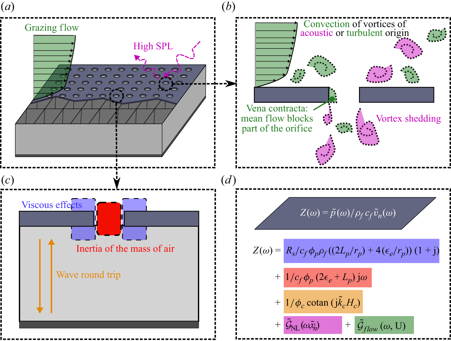
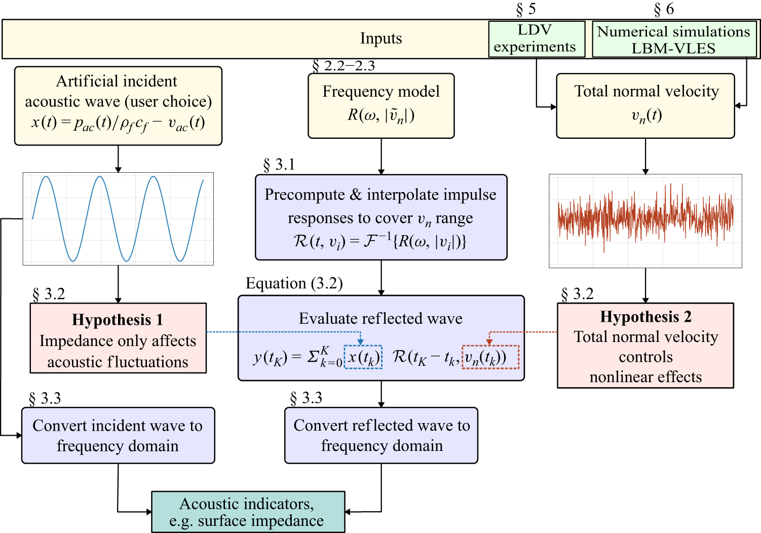
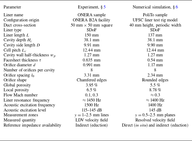
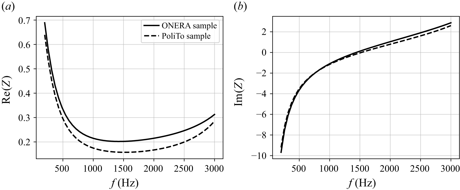
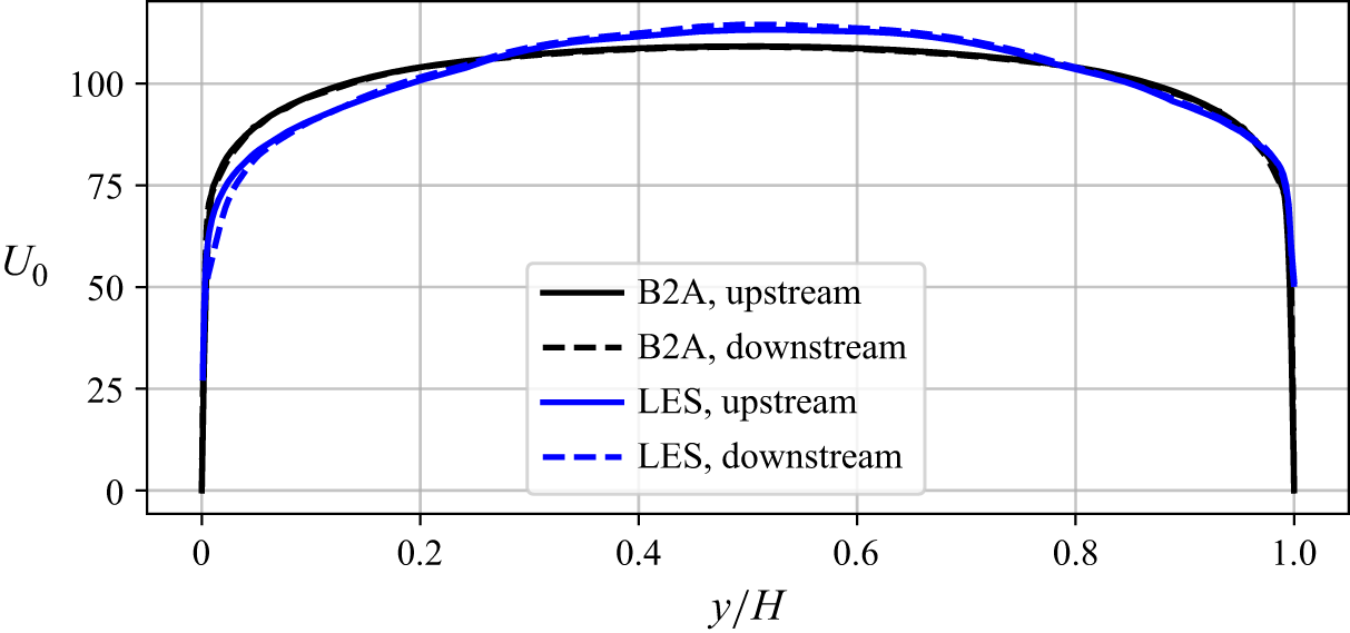
 y=0
 U0(0)=0
 y/H≳0.04

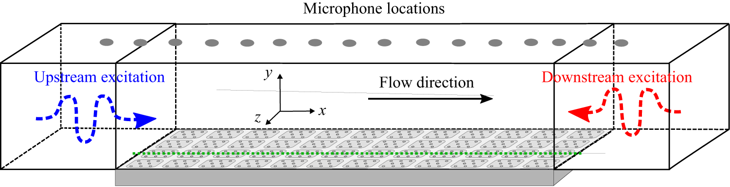
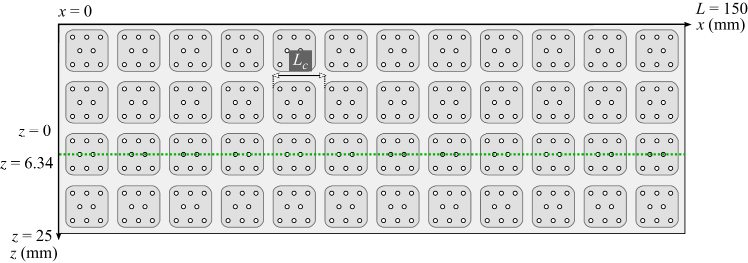
 Lc=12.44
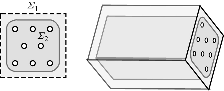
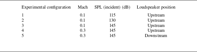
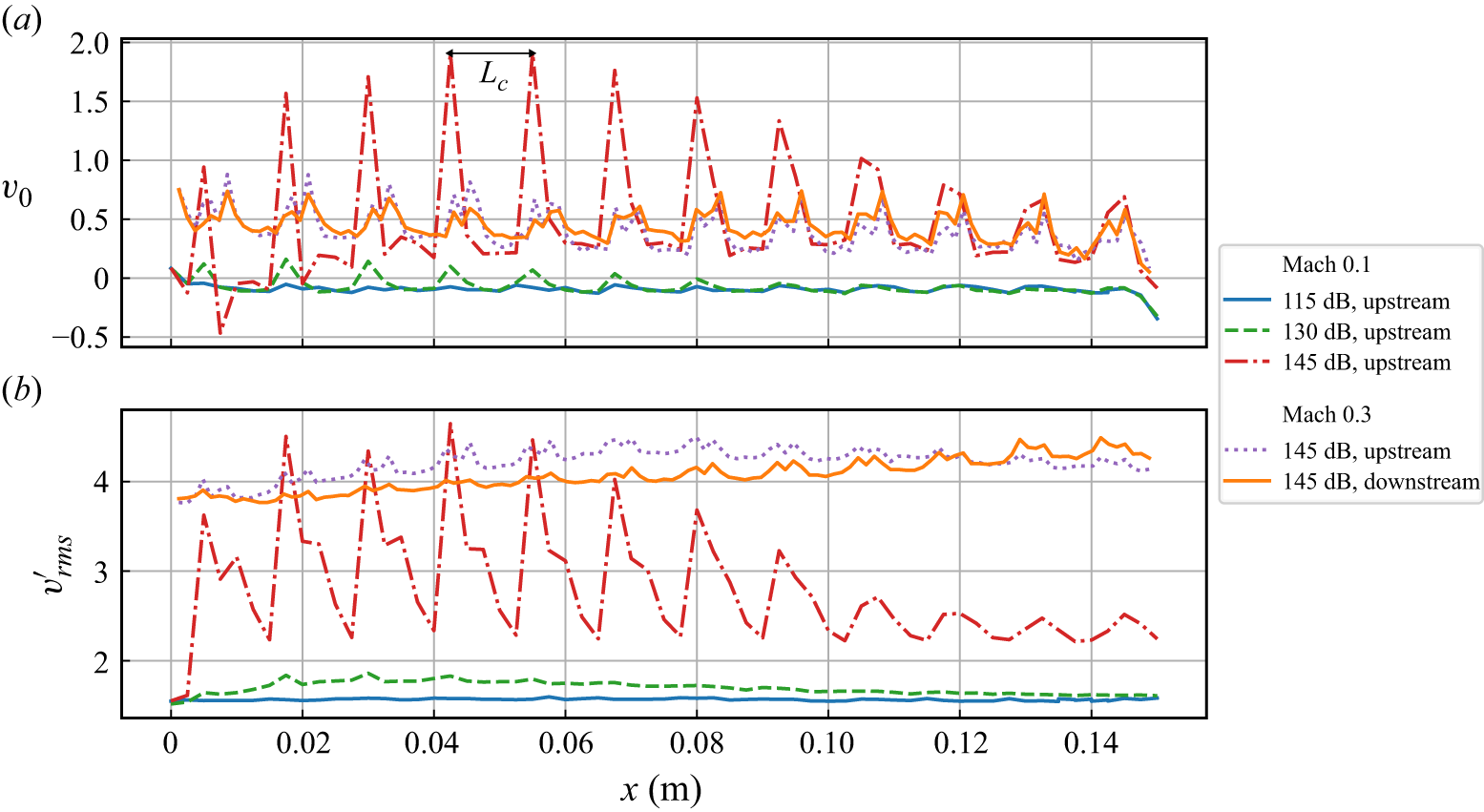
 Lc

 ±3

 ±3
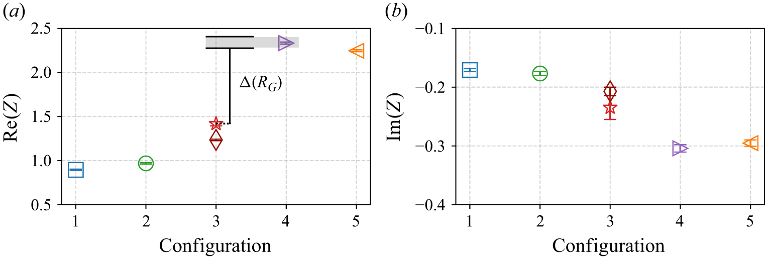
 Δ(RG)
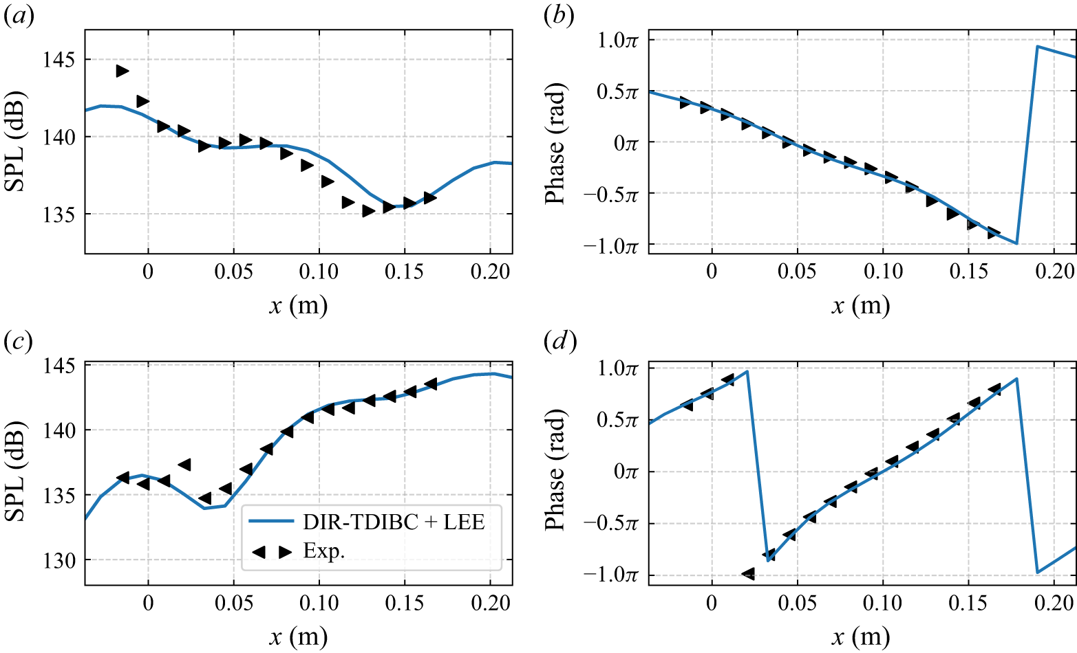
 x=0.437
 x=0.587
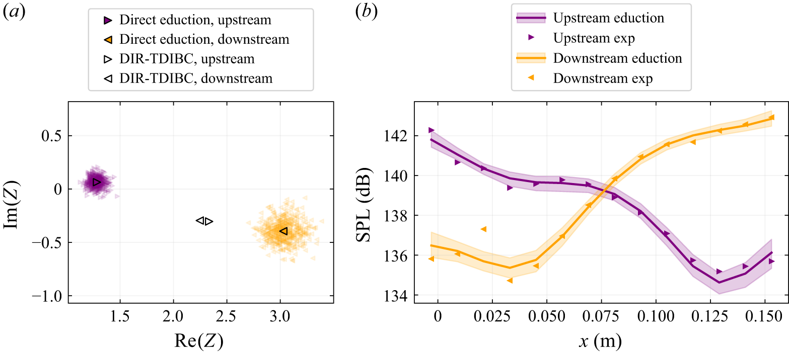
 x=0
 x=0.15m


 f
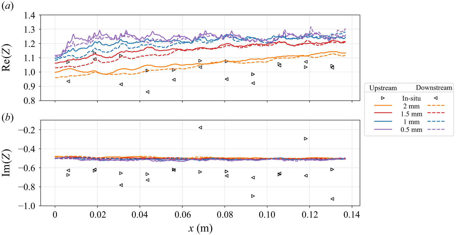
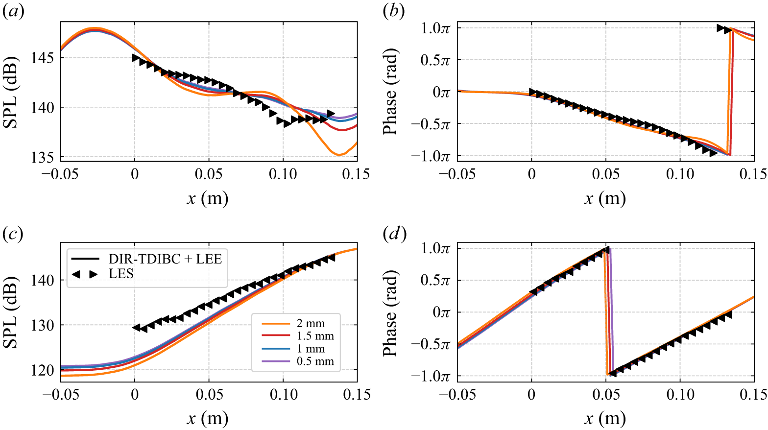
 x=0
 x=0.137
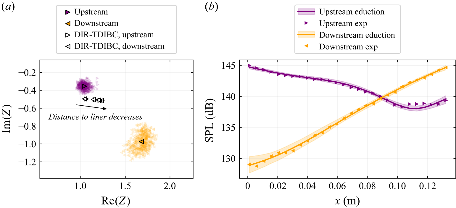
 145
 x=0
 x=0.137
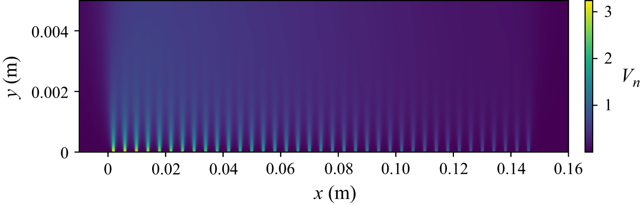
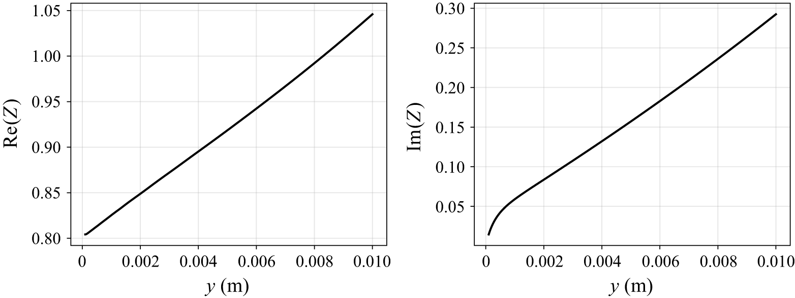
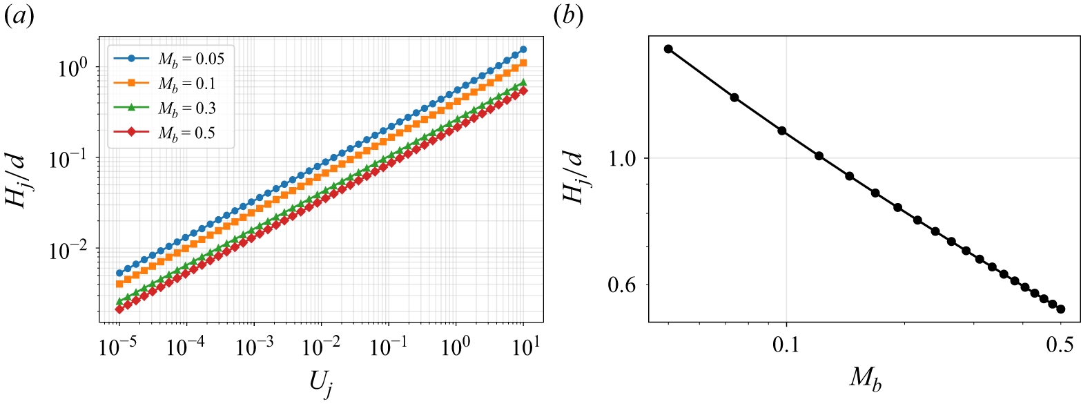
 δ=0.05
 Uj
 Hj
 Hj
 Uj=5ms−1

 Open access

