
Introduction
Since their discovery in 1970s[ Reference Whittingham 1 ] by M.S. Whittingham, with a lithium metal as anode and titanium (II) sulfide as cathode, there are exciting developments. In Whittingham's Li ion batteries, the anode being lithium metal has posed safety issues because pure lithium metal is more reactive. As a result of this, researchers tried to develop electrodes, which can contain Li ions (like intercalation compounds) and to improve the performance and safety of the Li ion batteries for new directions of applications.
After the notion of the use of Li ion batteries for electric vehicles, several additional factors such as safety, minimum time to charge and discharge (rate capability), and cycle life (durability) are becoming increasingly important. For this, new and advanced computational tools to predict battery properties are very important. Modeling is a key component of materials design. Especially for new materials with new material properties and new applications, virtual experimentation is a key to firsthand understanding and innovation. A model can allow interpreting experimental data, identifying rate limiting steps and predicting system behavior, while providing deeper understanding of the underlying physical processes. In materials engineering, several models have been at the forefront in the discovery and design of new materials. One of them is the phase field model. It is widely used for describing phase transformation and microstructural evolution.[ Reference Boettinger, Warren, Beckermann and Karma 2 – Reference Steinbach 5 ] Besides solidification, solid-state phase transformations and stress induced phase transformations,[ Reference Levitas and Roy 6 – Reference Momeni, Levitas and Warren 10 ] phase-field models are applied for simulating grain growth,[ Reference Chen and Yang 11 , Reference Miyoshia and Takaki 12 ] dislocation dynamics,[ Reference Chen and Hu 13 – Reference Wang, Liu and Zhuang 15 ] crack propagation,[ Reference Jin, Wang and Khachaturyan 16 , Reference Levine and Henry 17 ] solid state sintering[ Reference Patton, Kazaryan and Wang 18 – Reference Wang 20 ] and vesicle membranes in biological applications.[ Reference Du, Liu and Wang 21 , Reference Biben, Kassner and Misbah 22 ]
Phase field models, however, are relatively new to modeling electrochemical systems. Guyer et al. in 2004[ Reference Guyer, Boettinger, Warren and McFadden 23 , Reference Guyer, Boettinger, Warren and McFadden 24 ] first modeled the sharp electrode–electrolyte interface with a continuous phase field varying between 0 and 1, representing the liquid electrolyte and the solid metal phase, respectively. In this model, differential capacitance was simulated in accordance with experimental and density functional theory (DFT) data. There exist some phase field models to study electrode–electrolyte interfaces.[ Reference Pongsaksawad, Powell and Dussault 25 , Reference Shibuta, Okajima and Suzuki 26 ] Most of the electrochemical models described, use models applicable at equilibrium conditions and ignore non-equilibrium interactions especially at the beginning of interaction between two phases. A new finite interface phase field model, however, has been developed recently by Steinbach et al.[ Reference Steinbach, Zhang and Plapp 27 , Reference Zhang and Steinbach 28 ] which can handle processes across interfaces between two interacting materials at an arbitrary thermodynamic state. Preiss et al.[ Reference Preiss, Borukhovich, Alemayehu and Steinbach 29 ] extended the applicability of Steinbach's finite interface model for use in electrochemistry based on the OpenPhase framework.
In this work, kinetics investigation of the intercalation of electrode–electrolyte interface based on a new finite interface dissipation (FID) phase field model[ Reference Steinbach, Zhang and Plapp 27 , Reference Zhang and Steinbach 28 ] is described. Moreover, the FID phase field includes a contribution driven by diffusion potential difference between the two interacting phases (electrode and electrolyte) to the kinetics of charging and discharging. One parameter of paramount importance in the FID is the interface permeability. A more precise description of this quantity helps to gain a deeper understanding of the kinetics of redistribution at the interface between two interacting phases (materials). For this reason, a new approach to estimate the permeability of the interface for non-equilibrium electrochemistry was based on the Butler–Volmer kinetics.
Modeling method and procedures
Using the multiphase-field method, we begin with a general description of the free energy by integrating energy densities over a domain Ω. The grain boundary free energy density, f int, chemical free energy density, f chem, are integrated to obtain the total free energy
 $$F = \int\limits_\Omega {\{ f^{{\rm int}} + f^{{\rm chem}}\}} $$
The interfacial free energy density is given as
 $$f^{{\rm int}} = \displaystyle{{4\sigma _{\alpha \beta}} \over \eta} \left\{ { - \displaystyle{{\eta ^2} \over {\pi ^2}}\nabla \phi _\alpha \cdot \nabla \phi _\beta + \phi _\alpha \phi _\beta} \right\}$$
where σ αβ is the interface stiffness and η is the interface width. The field variable ϕ α is equal to 1 in the sub-domain α, where all other phase-fields are zero. At the interface ϕ α smoothly changes from 1 to 0. Furthermore, for every point in the space the sum of the phase-fields is constrained to 1;
 $$\phi _\alpha + \phi _\beta = 1$$
The overall concentration is given by a mixture rule.
 $$c(x,t) = c_\alpha (x,t)\phi _\alpha (x,t) + c_\beta (x,t)\phi _\beta (x,t)$$
where ϕ
α
and ϕ
β
are the phase fractions of phases α and β, respectively.
 $c_\alpha (x,t)$
and
 $c_\beta (x,t)$
are concentrations of phases α and β, respectively.
The chemical free energy density is
 $$f^{{\rm chem}} = \phi _\alpha f_\alpha (c_\alpha ) + \phi _\beta f_\beta (c_\beta ) + \lambda \{ c - (\phi _\alpha c_\alpha + \phi _\beta c_\beta )\} $$
The Lagrange multiplier λ, associated with the constraint of Eq. (4), is introduced to ensure solute conservation between the phases. The bulk free energies
 $\phi _\alpha f_\alpha (c_\alpha )$
and
 $\phi _\beta f_\beta (c_\beta )$
indicate the free energies of the individual phases. As described in,[
Reference Steinbach and Apel
30
] they may include stress-strain energy (Fig. 1). Here only the chemical free energy densities and the interfacial energy densities are considered.
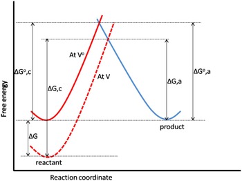
Effect of the overpotential on the free energies of activation for reduction and oxidation.

The concentration fields for the two interacting phases α and β is given explicitly by the sum of contributions from diffusion, permeation and phase transformation. For phase α in a two phase material, for example, the corresponding concentration evolution is given by Eq. (6)[ Reference Steinbach, Zhang and Plapp 27 ]
 $$\phi _\alpha \dot c_\alpha = \vec \nabla (\phi _\alpha D_\alpha \vec \nabla c_\alpha ) + P\phi _\alpha \phi _\beta (\mu _\beta - \mu _\alpha ) + \phi _\alpha \dot {\phi} _\alpha (c_\beta - c_\alpha )$$
P is the interface permeability, the inverse of the resistivity of the interface against diffusion. For more details of the derivation of Eq. (6), see Steinbach.[ Reference Steinbach 31 ]
The first part on the right hand side (RHS) of Eq. (6) describes Fick's diffusion driven by a spatial concentration gradient, scaled by the diffusion coefficient, D α . The second part describes redistribution of atoms inside the interface due to a diffusion potential difference scaled by the permeability. The third part of the equation describes a correction taking into account the mass conservation during the transformation driven by concentration difference between the phases, scaled by the phase field variable ϕ and its time derivative.
The evolution equation for the phase field ϕ
α
(
 $\dot {\phi} _\alpha $
=
 $ - \dot {\phi} _\beta $
) is given by a variational derivative of the total functional with respect to the phases.
 $$\dot {\phi}_\alpha = \displaystyle{{M_{\alpha \beta}} \over {2\eta}} \left\{ {\displaystyle{{\delta F} \over {\delta \phi _\alpha}} - \displaystyle{{\delta F} \over {\delta \phi _\beta}}} \right\}$$
where M αβ is the mobility of the interface.
The governing equation for the phase field evolution of phase α is given by
 $$\dot {\phi}_\alpha = K\left\{ {\sigma _{\alpha \beta} \left[ {\nabla ^2\phi _\alpha + \displaystyle{{\pi ^2} \over {\eta ^2}}\left( {\phi _\alpha - \displaystyle{1 \over 2}} \right)} \right] - \displaystyle{{\pi ^2} \over {8\eta}} \Delta g_{\alpha \beta} ^{\,phi}} \right\}$$
where
 $$K = \displaystyle{{2P\eta M_{\alpha \beta}} \over {2P\eta + M_{\alpha \beta} {(c_{\alpha \;} - c_\beta )}^2}}$$
with the driving force for phase transformation
 $g_{\alpha \beta} ^{\,phi} $
as a function of the chemical diffusion potentials
 $$\Delta g_{\alpha \beta} ^{\,phi} = \; f_\alpha - f_\beta + (\phi _\alpha \widetilde{\mu} _\alpha + \phi _\beta \widetilde{\mu} _\beta )(c_\alpha - c_\beta ).$$
Links to electrochemistry
The permeability, P shown in Eq. (6) describes the ease with which atoms (molecules) diffuse from one phase to the other in a certain volume element driven by the diffusional potential difference between the phases. Here the diffusional potential refers to the derivative of the Gibbs energy with respect to the concentration far from equilibrium. This triggers an additional flux proportional to P ϕ β to the concentration evolution equation for phase α as shown in Eq. (6).
Let us now focus more on the second part of Eq. (6) because that is where the novel feature of this model exists. Published phase field models[ Reference Boettinger, Warren, Beckermann and Karma 2 , Reference Tiaden, Nestler, Diepers and Steinbach 32 – Reference Boettinger and Warren 37 ] are usually based on diffusion and phase transformation. Although there are some phase field models that describe processes that are far from equilibrium, most of them use already developed phase diagram data for alloys and equilibrium partitioning condition to study the kinetics and they fail to explicitly describe the evolution of the component exchange between the phases (materials) in a kinetic equation that links the concentration fields of the phases. The main advantage of this model is, therefore, the possibility to investigate relaxation kinetics for two interacting phases (materials) far from equilibrium across the interface, which is very suitable to model Solid Electrolyte Interface (SEI) in an electrochemical system. This can also be observed e.g., in solute trapping or the transition to partitionless transformation in rapid solidification.[ Reference Gahn and Baker 38 , Reference Kittl, Sanders, Aziz, Brunco and Thompson 39 ]
As our aim is to link phase field with electrochemistry for investigation of electrode– electrolyte intercalation, let us now obtain an expression for this quantity under microscopic considerations. For this purpose, we will evaluate the total number of solute atoms that ‘jump’ between the two phases for a stationary interface in two different ways. As derived in detail in the original publication,[ Reference Steinbach, Zhang and Plapp 27 ] let us first consider the second term in Eq. (6),
 $$\phi _\beta \dot c_\beta = P\phi _\alpha \phi _\beta \left( {\displaystyle{{\partial f} \over {\partial \phi _\alpha}} - \displaystyle{{\partial f} \over {\partial \phi _\beta}}} \right)$$
which represents the composition change in the β phase due to the atoms that ‘arrive’ from the α phase. In order to transform this into an expression for the number of solute atoms per unit volume that cross the interface per unit time, let us divide both sides of the equation by the molar volume V m. Next, to obtain the total number of atoms that cross an area dA of the interface, the resulting expression needs to be integrated over that surface element as well as across the interface, since atoms jump from one phase to the other over the whole width of the interface. Under the assumption that the chemical potentials are constant in both phases within the interfacial region, and using the expression for the equilibrium profile of the phase fields, this integration yields
 $$\dot n_\beta = \; \displaystyle{{\eta P} \over {8V_m}}(\mu _\alpha - \mu _\beta ){\rm d}A$$
with n
β
the number of solute atoms in units of moles. From a dimensional point of view,
 $\; \dot n/{\rm d}A$
is the current density of solute atoms that crosses the interface.
The electrical current density across the interface, due to the intercalation reaction, I αβ determines the ion flux as well as the electric current due to the transport of Lithium ions through the electrode–electrolyte interface (Fig. 2). Hence, the number of atoms that cross a surface of area dA per unit time of Lithium ions, which crosses the electrode–electrolyte interface would be[ Reference Wang and Sastry 40 – Reference Bazant 42 ]
 $$\displaystyle{{\dot n} \over {{\rm d}A}} = \; \displaystyle{{I_{\alpha \beta}} \over {zF}}$$
where z is the number of charges, which is one in our case and F is the Faraday's constant.
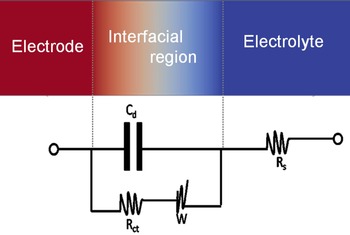
An equivalent circuit of an electrode–electrolyte interface.

Combining Eqs. (12) and (13) and solving for P, one can obtain an interface permeability P, which is directly related to the current density.
 $$P = \displaystyle{{8V_{\rm m}I_{\alpha \beta}} \over {zF\eta (\mu _\alpha - \mu _\beta )}}$$
If the chemical potentials μ are given in J/m3, then P has the unit m3/J/s. Equation (14) is very important in that not only does it connect the permeability with the electrical current density, but it also helps to get a direct access to experimental measurements. For an electrochemical system where only one active species is involved like Li in Li
x
FePO4, the current density that crosses a certain interface is given by a current density vector
 ${\hat i}$
that points from one phase to the other and with a normal
 $$\; I = \hat i \cdot \hat n$$
where the normal
 $\hat n$
points from α into β. Let us denote the partial current densities at the anode and cathode as
 $\vec i $
and
 $\overleftarrow i $
, respectively. Considering the reaction described in Eq. (16) at the interface of the electrolyte and solid electrode phase,
 $$\; Li_xm\rightleftharpoons xLi^ + + m + xe^ - $$
where Li+ represents a lithium ion in the electrolyte, x is the number of lithium atoms and m represents the matrix phase. If the forward (de-intercalation) reaction of Eq. (16) is of first order with respect to the concentration of Li+ that is leaving the electrode, the rate of concentration change is given by[ Reference Wang and Sastry 40 – Reference Bazant 42 ]
 $$\displaystyle{{\dot n} \over {{\rm d}A}} = \displaystyle{{I_\beta} \over {zF}}$$
which means that the forward current density
 $\vec i $
can be written as
 $$\vec i = zF\dot n_\alpha $$
In a similar fashion, the backward current density
 $\overleftarrow i $$
 $$\overleftarrow i = zF\dot n_\beta $$
The rate of the forward reaction if first order with the species concentration is given by
 $$\dot n_\alpha = k_{\rm f}c_\alpha $$
and
 $$\dot n_\beta = k_{\rm b}c_\beta $$
where k f and k b are the forward and backward heterogeneous rate constants, respectively. These constants depend on the operating potential according to the Arrhenius relationship:
 $$k_{\rm f} = k^{\rm o}e^{ - (\alpha zF/RT)(V - V^{\rm o})}$$
 $$k_{\rm b} = k^{\rm o}e^{((1 - \alpha )zF/RT)(V - V^{\rm o})}$$
where k
o is the standard rate constant, α is the transfer coefficient and
 $(V - V^{\rm o})$
is the operating potential, which is considered the activation energy in this case. The value of α (between zero and unity) reflects the symmetry of the free energy curve (with respect to reactants and products). For symmetric curves, α will be close to 0.5; α is a measure of the fraction of energy that is put into the system used to actually lower the activation energy. Equations (22) and (23) indicate that by changing the applied potential, one can influence k
f and k
b in an exponential fashion.
Hence, the forward and backward current densities are generally given, respectively, by the following equations:
 $$\vec i = zFk_{\rm f}c_\alpha $$
 $$\overleftarrow i = zFk_{\rm b}c_\beta $$
The net current density that crosses the electrode–electrolyte interface is the current coming in and the current leaving out, which is the difference of the anodic and cathodic current densities.
 $$I_{\alpha \beta} = {\vec i} - {\overleftarrow i}$$
 $$= zFk_{\rm f}c_\alpha - zFk_{\rm b}c_\beta$$
 $$= zFk^{\rm o}(c_\alpha e^{ - (\alpha zF/RT)(V - V^{\rm o})} - c_\beta e^{((1 - \alpha )zF/RT)(V - V^{\rm o})})$$
At equilibrium,
 $\vec i\, =\, \overleftarrow i $
and setting I
αβ
= 0 from Eq. (28), we have
 $$c_\alpha e^{ - (\alpha zF/RT){(V - V^{\rm o})}_{{\rm eq}}} = c_\beta e^{((1 - \alpha )zF{\rm /}RT){(V - V^{\rm o})}_{{\rm eq}}}$$
Solving for
 $(V - V^{\rm o})_{{\rm eq}} = E_{{\rm eq}}$
from Eq. (29), we have the following relation
 $$E_{{\rm eq}} = \displaystyle{{RT} \over {zF}}\ln \left( {\displaystyle{{c_\alpha} \over {c_\beta}}} \right)$$
And hence the equilibrium current density i o becomes
 $$i_{\rm o} = zFk^{\rm o}c_\alpha e^{ - (\alpha zF/RT)E_{{\rm eq}}} = zFk^{\rm o}c_\beta e^{((1 - \alpha )zF/RT)E_{{\rm eq}}}$$
Normalizing I αβ by i o, and using Eqs. (28) and (31) we have
 $$\displaystyle{{I_{\alpha \beta}} \over {i_{\rm o}}} = \displaystyle{{\vec i} \over {i_{\rm o}}} - \displaystyle{{\overleftarrow i} \over {i_{\rm o}}}$$
 $$\!\!\!\!\!\!\!= \displaystyle{{zFk^oc_\alpha e^{ - {{\alpha zF} \over {RT}}E}} \over {zFk^oc_\alpha e^{ - {{\alpha zF} \over {RT}}E_{eq}}}} - \displaystyle{{zFk^oc_\beta e^{ -{{(1 - \alpha )zF} \over {RT}}E}} \over {zFk^oc_\beta e^{ -{{(1 - \alpha )zF} \over {RT}}E_{eq}}}}$$
 $$= e^{ - (\alpha zF/RT)(E - E_{{\rm eq}})} - e^{((1 - \alpha )zF/RT)(E - E_{{\rm eq}})}$$
When anodic polarization (Polarization is the kinetic variation from equilibrium voltage. Also called overpotential.) is appreciable, the cathodic current density is exceedingly low and practically, one can assume that
 $I = \vec i $
; when cathodic polarization is appreciable, one can assume that
 $I = \overleftarrow i $
. By re-writing Eq. (34), one obtains the Butler–Volmer equation.
 $$I_{\alpha \beta} = i_0(e^{(\alpha _{\rm a}zF/RT)\psi} - e^{( - \alpha _{\rm c}zF/RT)\psi} )$$
where i o is the exchange current density, A/m2, α a and α c are transfer coefficients for the anode and cathode respectively, usually the cathodic reaction is symmetric with anodic reaction and hence α a = α c. F is Faraday's constant, R is the gas constant, T is the temperature and ψ = E − E eq is the overpotential.
The first term inside the brackets represents the anodic/oxidizing reaction and the second term represents the cathodic/reducing reaction. i
o in Eq. (35) describes the equilibrium current density. At equilibrium, the anodic and cathodic partial current densities are equal. This means that the net current density that is described in Eq. (28) is zero. i.e.,
 $\vec i = \overleftarrow i $
. Equilibrium, however, does not mean there is no flux of atoms, but rather the flux of atoms that are entering an interface are equivalent with the flux of atoms leaving the interface. In terms of current densities, at equilibrium, the cathodic current density is equal to the anodic one and is given by the exchange current density.
 $$\vec i \,= \,\overleftarrow i \; = i_{\rm o}$$
Using the equilibrium voltage in Eq. (30), i o can analytically be expressed as
 $$i_{\rm o} = \vec i \,=\, \overleftarrow i $$
 $$= zFk^{\rm o}c_\alpha e^{ - (\alpha zF/RT)E_{{\rm eq}}}$$
 $$= zFk^{\rm o}c_\alpha e^{( - \alpha zF/RT)(RT/zF)\ln (c_\alpha /c_\beta )}$$
 $$= zFk^{\rm o}c_\alpha \left( {\displaystyle{{c_\alpha} \over {c_\beta}}} \right)^{ - \alpha} $$
Since the current density is driven by the flux of Li into the electrode and this flux is proportional to the rate constant and concentration of Li in the electrode and electrolyte, the exchange current density in Eq. (35) can also be described in simpler expressions using Eq. (40) in terms of concentration of Li in the electrode (c β ) in the electrolyte (c α ) by the following expression.
 $$i_{\rm o} = K_{\rm e}(c_\alpha )^{1 - \alpha} (c_\beta )^{ - \alpha} $$
where c α and c β are the concentration of Li in the electrode and electrolyte, respectively. The transfer coefficient α = α a = α c = 0.5. K e is an experimental parameter determined from electrochemical measurements.
The maximum concentration of Li, c α ,max in Li x m is when x = 1. i.e., complete intercalation. To calculate Li concentration in atom% in Li x FePO4, for example, is
 $$c = \displaystyle{x \over {x + 6}} \cdot 100\% $$
where the number 6 indicates the number of non-Li atoms in the compound. Now when x = 1, c α ,max ≈ 14.3 atom%.
Assuming that the electrode can only accommodate a maximum concentration of Li, c
α,max, the number of surface sites available for adsorption after absorbing c
α
concentrations is
 $(1 - (c_\alpha /c_{\alpha, \max} ))$
. The characteristic curve of the permeability is also affected by the behavior of the exchange current density.
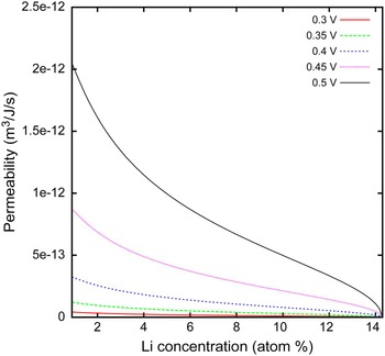
A higher overpotential drives more electrons to redistribute between the electrode and electrolyte. As can be seen from Fig. 5 increasing the overpotential, increases the permeability of the interface.
The exchange current density is measured experimentally by cyclic voltammetry (CV)[ Reference Noel and Rajendran 43 , Reference Flandrois 44 ] or impedance spectroscopy.[ Reference Macdonald 45 – Reference Wang and Hong 48 ] Going into the details of Eq. (35), let
 $$y = \displaystyle{{\alpha _{\rm a}F} \over {RT}}\psi $$
for y ≪ 1, by Taylor expansion
 $$e^y \approx 1 + y$$
which implies that the Butler–Volmer relationship described in Eq. (35) simplifies to
 $$I = 2i_{\rm o}\displaystyle{{\alpha _{\rm a}F} \over {RT}}\psi. $$
Using α a = α c = α = 0.5, Eq. (45) results in
 $$I = i_{\rm o}\displaystyle{F \over {RT}}\psi. $$
For a very small overpotential, the charge transfer resistance, R ct [ Reference Vielstich, Hamann and Hamnett 49 , Reference Zhu and Wang 50 ] is defined by
 $$R_{{\rm ct}} = \displaystyle{{{\rm d}\psi} \over {{\rm d}I}}.$$
Using Eqs. (46) and (47), the charge transfer resistance is given by
 $$R_{{\rm ct}} = \displaystyle{{RT} \over {i_{\rm o}F}}.$$
This means that the interface permeability is inversely proportional to the charge transfer resistance. Equation (48) gives an insight to the estimation of the permeability of the interface with experimentally accessible electrochemical quantities. R ct is determined from Impedance Spectroscopy (IS) measurements. IS is an effective technique for probing the features of chemically modified electrodes and for understanding electrochemical reaction rates.[ Reference Lasia 47 , Reference Katz and Willner 51 ] Impedance is the measure of the opposition that a circuit presents to a current when a voltage is applied. In quantitative terms, it is the complex ratio of the voltage to the current in an alternating current circuit and possesses both magnitude and phase, unlike resistance, which has only magnitude. Electrochemical transformations occurring at the electrode–electrolyte interface can be modeled using components of the electronic equivalent circuitry that correspond to the experimental impedance spectra. Particularly useful to model interfacial phenomena is the Randles and Ershler electronic equivalent circuit model (Fig. 3).[ Reference Vielstich, Hamann and Hamnett 49 ] This includes the double layer capacitance C d, the ohmic resistance of the electrolyte solution R s, the charge transfer resistance R ct and the Warbung impedance W resulting from the diffusion of ions from the bulk electrolyte solution to the electrode surface. The impedance of the interface Z(ω), derived by application of Ohm's law, consists of two parts, a real Z′ and an imaginary Z′′
 $$\eqalign{Z(\omega ) & = R_{\rm s} + \displaystyle{{R_{{\rm ct}}} \over {(1 + \omega ^2R_{{\rm ct}}^{\rm 2} C_{\rm d}^{\rm 2} )}} - j\displaystyle{{\omega R_{{\rm ct}}^{\rm 2} C_{\rm d}} \over {(1 + \omega ^2R_{{\rm ct}}^{\rm 2} C_{\rm d}^{\rm 2} )}} \cr & = Z{\rm ^{\prime}} + jZ^{\rm \prime\prime}}$$
where j 2 = −1 and ω is radial frequency (expressed in radians/second) from which the real and imaginary parts, respectively, are
 $${\mathop{\rm Re}\nolimits} (Z) = Z{\rm ^{\prime}} = R_{\rm s} + \displaystyle{{R_{{\rm ct}}} \over {(1 + \omega ^2R_{{\rm ct}}^{\rm 2} C_{\rm d}^{\rm 2} )}}$$
and
 $$\left \vert {{\mathop{\rm Im}\nolimits} (Z)} \right \vert = \left \vert {Z^{\rm \prime\prime}} \right \vert = \displaystyle{{\omega R_{{\rm ct}}^{\rm 2} C_{\rm d}} \over {(1 + \omega ^2R_{{\rm ct}}^{\rm 2} C_{\rm d}^{\rm 2} )}}$$
The Impedance shown in Eq. (49) has both magnitude and phase, where the latter is given by
 $$\varphi = \displaystyle{{{\mathop{\rm Re}\nolimits} (Z)} \over {{\mathop{\rm Im}\nolimits} (Z)}}$$
We can also obtain the following limiting values from Eq. (49):
 $$\omega \to 0:{\mathop{\rm Re}\nolimits} (Z) \to R_{\rm s} + R_{{\rm ct}};\;{\mathop{\rm Im}\nolimits} (Z) \to 0$$
 $$\omega \to \infty :{\mathop{\rm Re}\nolimits} (Z) \to Rs;\;{\mathop{\rm Im}\nolimits} (Z) \to 0$$
 $$\omega = \displaystyle{1 \over {(R_{{\rm ct}}C_{\rm d})}}:{\mathop{\rm Re}\nolimits} (Z) = R_{\rm s} + \displaystyle{{R_{{\rm ct}}} \over 2};\;{\mathop{\rm Im}\nolimits} (Z) = \displaystyle{{R_{{\rm ct}}} \over 2}$$
By re-writing the equation for the current density in terms of the charge transfer resistance shown in Eq. (48) and inserting in Eq. (14), one gets
 $$P = \displaystyle{{8V_{\rm m}(RT/FR_{{\rm ct}})} \over {zF\eta (\Delta \mu )}}$$
 $$= \displaystyle{{8V_{\rm m}i_{\rm o}} \over {zF\eta (\Delta \mu )}}$$
R ct is calculated from an equivalent circuit diagram by IS. The exchange current density can be determined experimentally both by CV and IS. By CV, one can measure the exchange current density versus potential and the potential versus the concentration of Li.[ Reference Noel and Rajendran 43 , Reference Zhu and Wang 50 ] The above two ways to get the current density were based on low overpotential, which means that the system is near to equilibrium. However; under high overpotential, most electrochemical systems are far away from equilibrium. And hence new ways to estimate parameters are required. Working more on Eq. (35) and assuming that the transfer coefficients α a and α c are equal i.e., α a = α c = 0.5, let us simplify Eq. (35) to the following form.
 $$I_{\alpha \beta} = 2i_{\rm o}\sin h(a\psi )$$
where a = 0.5F/RT.
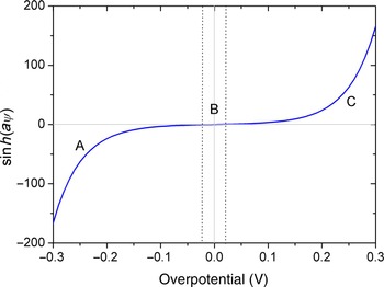
The variation of
 $\sin h(a\psi )$
with respect to the overpotential, ψ. The different regions labeled as A, B and C indicate negative influence, no influence, and positive influence of the overpotential on the current density, respectively.

From Fig. 4, we can see that the total range of potential can be divided into three regions: one region at low values of overpotential (to both sides of the equilibrium potential (B)), where the two partial reactions occur at comparable rates and two regions at high values of anodic and cathodic polarizations, where the reverse partial reactions can be neglected (shown as regions A and C). The two experimental ways of determining the current density, CV and IS, work well when the overpotential is less than 20 mV because as can be seen from Fig. 4, the factor for the exchange current density is negligible for very low value of positive and negative overpotentials. A slight change after this minimum overpotentials results in a drastic increment of this factor, which also affects the permeability of the interface.
Permeability of the interface with Li concentration in the electrode. Li concentration in the electrolyte was set to be 0.58 at.%. i o was estimated using K e = 6.37 × 10⁻⁴. The different colors show calculations at different overpotentials.

Depending on the type of material used, different electrode materials have different overpotentials. The rate of intercalation is sensitive to the overpotential of the electrode and as described in Eq. (46), a higher overpotential results in a higher current density, which also means that an increased overpotential increases the permeability at a certain current density.
The higher the overpotential of the electrode, the higher the driving force for redistribution of the atoms at the interface resulting in higher interface permeability. This means that the overpotential facilitates the redistribution due to high number of electron difference between the electrode and electrolyte. Figure 5 shows concentration dependent interface permeability calculated at different overpotentials.
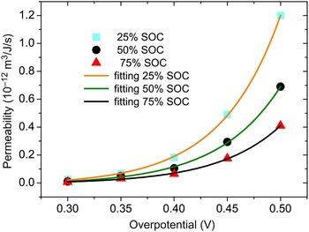
Permeability of the interface versus the overpotential at different SOC. Solid lines show the fitting curves and data sets are shown by different geometries.

At a certain overpotential, the permeability decreases with increasing concentration of Li. This could be due to the filling up of the spaces for the electrode material. Initially the permeability is higher. This is because of the free space available for redistribution of Li in the electrode. As intercalation proceeds, more Li piles up near the surface of the electrode thereby increasing the activation energy for redistribution, which ultimately diminishes the rate of redistribution.
The characteristic curve of the interface permeability with concentration of Li in the electrode is attributed to the characteristic curve of the current density. A more precise description of the current density gives rise to more precise interface permeability, which ultimately helps to capture the magnitude of the rate of redistribution at the interface between the electrode and electrolyte. The current density is a function of Li concentration. As the current density can be determined experimentally by CV or IS, it can also be estimated from equilibrium reaction rate theory as shown in Eq. (41). There is a non-linear relationship between the permeability of the interface and the overpotential. An exponential fit of the data gives a very good agreement to the calculated permeability. As portrayed in Fig. 6, an increase in the overpotential results in a monotonously exponential increase in the permeability of the interface. This is due mainly to the high rate of Li flux activated by the higher overpotential. There is a very good agreement between the exponential fit and calculated values of the permeability of the interface at a particular state of charge.
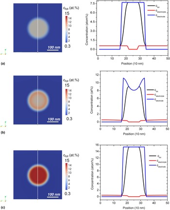
Simulation result of concentration evolution of a single spherical particle immersed in an electrolyte solution of LiPF6. The figures on the right show concentration profile at different time steps by line scan as shown in the slide view.

As shown in Fig. 6, the permeability of the interface varies exponentially with the overpotential with a form of the function
 $$P = y_{\rm o} + Ae^{\psi /t_1}$$
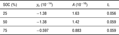
where P and ψ are the permeability and the overpotential, respectively. y o, A and t 1 are fitting parameters, which are given in Table I at different state of charge (SOC).
The values of the constant t 1 at different SOC are comparable as shown in Table I. The exponential relationship arises from the Butler–Volmer description of the current density. The current density is exponentially related to the overpotential. And the permeability of the interface is proportional to the current density as described by Eq. (14). This makes the permeability to be an exponential function of the overpotential. This means at a certain SOC, the permeability of the interface increases exponentially as the overpotential increases, which ultimately enhances the rate of flux due to redistribution of Li. This is due to the higher degree of disorder between the Li ions at higher over potential.
Fitting parameters at different SOC.

Simulation procedure
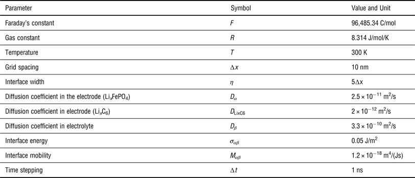
The process of diffusion and partitioning in the non-stoichiometric electrode phase of Li x FePO4 in an electrolyte solution of Li x PF6 has been simulated using our open source package for phase-field modeling and simulations. A cubic domain of 100 × 100 × 100 grid points with a grid spacing of 10 nm and the interfacial width of 50 nm was simulated. The diffusivity of Li in the corresponding phases was obtained from published literature. The energy density of the electrode was obtained from electrochemical voltage versus Li content measurements and is described in the next section. Other input parameters required for the simulation are described in Table II.
Input parameters for simulation of a spherical Li x FePO4 particle.

Chemical energy
For any thermodynamic system, the Gibbs energy is the sum of the contributions from the internal energy and entropy.
 $${\rm d}G = {\rm d}U - T{\rm d}S - S{\rm d}T + V{\rm d}p$$
where U is the internal energy, S is the entropy, T is the temperature and p is the pressure of the system. V is the volume of the system.
And the internal energy is given by
 $${\rm d}U = T{\rm d}S - (\,p{\rm d}V + {\rm d}W_{{\rm elec}})$$
where the expression inside the bracket describes the sum of electrical work done and the mechanical work done due to volume change. This makes the Gibbs energy to have the following form of expression
 $${\rm d}G = - S{\rm d}T + V{\rm d}p - {\rm d}W_{{\rm elec}}$$
which means that at constant temperature and pressure, the Gibbs energy is negative of the electrical work. Since there is no concentration dependent eigenstrains in the materials we consider, only the total chemical energy contribution is considered for the current model. There are, however, materials that have concentration dependent eigenstrains and their contribution to the flux can easily be incorporated in the pressure term in the above equations.
For electrochemistry, the potential of the system to perform electrical work is measured by the voltage also called the electrical potential. The electrical work done to move a charge Q through an electrical potential E is given by multiplying the number of charges by voltage and Faraday's constant.
 $${\rm d}W_{{\rm elec}} = - zF{\rm d}E$$
where z is the number of charges and is positive one for Li ion. F is Faradays constant, which has a value of 96,485.34 C/mol.
By combining the Eqs. (62) and (63) at constant pressure and temperature, one can obtain that the Gibbs energy is
 $$\Delta G = - zF\Delta E$$
where ∆E is the deviation of the voltage from the equilibrium voltage i.e., ∆E = E–E eq.
Most electrochemical measurements are based on voltage versus Li content. The beauty of Eq. (64) is, therefore, its importance in accessing the Gibbs energy from experimental measurements. Hence, ∆G can be extracted from electrochemical measurement results of the potential versus Li content. The change in potential difference between the electrodes and the electrolyte is the driving force for Li to (de)intercalate out of/into the electrodes.
Now let us bring our attention to how to model the electrode–electrolyte interface using the finite interface. As described previously, to model electrode and electrolyte interface, one needs to have the free energies of the electrode and the electrolyte (f α and f β for the electrode and electrolyte, respectively). With the help of Eq. (64) and electrochemical voltage versus Li content measurements as performed in,[ Reference Paolo, Lisi, Zane and Pasquali 52 ] one can obtain the chemical energy for the electrode (f α ). The free energy for the electrolyte solution is obtained by ideal solution approximation. Other computational and material related input materials are given in Table II.
Results and discussion
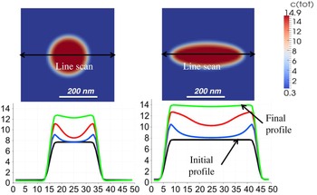
After careful parameterization of the new material parameter dubbed permeability of the interface and its relationship with electrochemical bulk properties, we now take a look at our simulation results. Let us consider a spherical electrode particle in contact with an electrolyte. We can treat the electrode and electrolyte as a solid and a liquid phase, respectively. The electrode is denoted as phase alpha (α) and the electrolyte is denoted as phase beta (β). With the diffuse interface model, the concentration of Li varies smoothly across the interfacial region. In this finite interface dissipation model, the concentrations of the phases are linked by a kinetic equation, which describes the exchange of components between the phases [Eq. (6)] instead of the condition of equal diffusion potential or an equilibrium partitioning condition. The parameter P, which was introduced earlier plays this role. As shown in Fig. 7, the active particle is immersed in an electrolyte solution in a periodic box. The phase field variable is set to have a sinusoidal value and the concentration evolutions of the components in the corresponding phases are calculated. In Fig. 7, the concentrations of each phase and the total concentration from the simulation are shown. The red color in the right side of the line scan plots show the concentration of Li in the electrolyte and the blue shows the concentration of Li in the electrode (active particle). The total concentration is indicated by the black line. The concentration of the electrolyte in the bulk of the active particle is zero and the concentration of Li in the bulk of the electrolyte is zero. The concentration at the interface is a weighted mean of the concentration of the corresponding phases by the phase fractions. That is why the concentration profiles smoothly vary from one phase to the other inside the interface.
Concentration [at.%] versus position [grid step] of a spherical and an ellipsoidal particle along the z-axis; different curves show concentration profile after every 105 steps.

The starting concentrations for the finite interface dissipation model can be any arbitrary concentrations. However; for this simulation, an electrolyte starting concentration of 0.58 at.% was used. The initial concentration of Li in the electrode particle was set to be 7.69 at.% which is equivalent to 50% SOC or Li0.5FePO4. As shown in Fig. 7(a), the initial concentration profile of a 100 nm radius Li x FePO4 particle with an initial concentration of 7.69 at.% in a 1 mol/L electrolyte salt solution of LiFP6 is shown. The simulation in Fig. 7 shows the concentration evolution after 0.15 ms. As can be seen from the figure, initially the Li concentration in the electrode was 7.69 at.%. With increasing time, more Li intercalates into the surface of the electrode particles and into the bulk of the particles. The first rapid increment in the Li concentration is due to redistribution and diffusion. As more Li intercalates into the electrode particle, the concentration in the electrode increases first near the vicinity of the interface and then further into the bulk. As time increases, more Li piles up near the vicinity of the surface of particles creating a concentration gradient between the surface and the bulk, which finally leads to a driving force for diffusion of species from the surface into the bulk of the active particle. The concentration of Li in the bulk of electrolyte is set to stay constant. The concentration variation near the vicinity of the interface is much higher than in the bulk of the active particle. This is mainly due to the additional contribution of the redistribution phenomenon. Redistribution, which is driven by the diffusional potential difference between Li in the electrode and Li in the electrolyte acts in the interface. This is clearly visible in the concentration profile plots of Fig. 7(b). Furthermore; the diffusion coefficient of Li in the electrolyte is two orders of magnitude higher than diffusion coefficient of Li in the electrode as shown in Table II. Further intercalation leads to the complete fill up of the active particle sites for Li. That is called a saturation condition or in battery terms a 100% full charge. For example, in Li x FePO4, a fully charged cathode is that the x in Li x FePO4 is 1 or the concentration of Li is 14.3 at.%. This is clearly observed in the simulation result of Fig. 7(c) where a saturation occurs at a Li concentration of 14.3 at.%. Saturation does not necessary mean equilibrium because for equilibrium the chemical potentials of the two phases have to be equal. It is, however, true that as more Li intercalates into the active particle, the potential of the electrode decreases (this works for a one phase assumption with a monotonic Gibbs energy function of the electrode with respect to Li concentration).
Influence of particle morphology
Depending on the type of manufacturing methods, the morphology of active particles can be tuned to a suitable application. For instance, different morphologies of FePO4 particles were prepared by Wang et al.[ Reference Wang, Wang, Liu, Cheng, Si and Geng 53 ] They produce different microstructures with controlled morphologies at relatively low temperature through kinetic manipulation. They observed morphology evolution during the experiments directly. The morphologies were mainly determined by the amount of the H3PO4 in the reaction system and changed from rugby to porous microsphere through controlling the concentration of H3PO4.
Moreover, Ellis et al showed crystal structure and electrochemical properties of A2MPO4F fluorophosphates (A = Na, Li, M = Fe, Mn, Co, Ni).[ Reference Ellis, Michael Makahnouk, Rowan-Weetaluktuk, Ryan and Nazar 54 ] They showed new solid state and hydrothermal synthetic routes to (Li,Na)2FePO4F that incorporate carbon containing additives and result in good electrochemical properties of Li (or Na) ion electrode material. A review on the solid-state chemistry and nanostructuring of materials that are conceptually providing new opportunities for tailored design of different electrode materials is given by Ellis et al.[ Reference Ellis, Lee and Nazar 55 ] They have also showed how the intrinsic properties of LiFePO4 can be modified with carbon coating. This helps to design specific morphologies of active particles for specific applications. In this work, a systematic investigation of the influence of the shape of particles on the kinetics of intercalation was performed. Particles of different shapes at constant surface area were considered. To investigate the influence of one parameter, other parameters are kept constant.
A spherical and an ellipsoidal electrode particle with the same material parameters were considered. From Fig. 9, one can observe that the concentration of Li varies at a higher rate for ellipsoidal particles. This is shown by the concentration versus time plot in the RHS of Fig. 9. The black curve in Fig. 9 shows the initial concentration of the electrode particle, which in this case is 7.69 at.% Li. That means half of the sites for Li in the active particle are filled. Upon discharging, more Li intercalates into the active cathode particle by diffusion and redistribution at the interface. After the first 105 steps, we can see a significant increment of Li concentration especially at the vicinity of the interface and is shown by the blue curve. This is because of the diffusion of Li from the electrolyte into the electrode particle. The significant increment of concentration across the interface is due to the effects of redistribution and diffusion. The concentration increment at the same time step is higher for the ellipsoidal particle. This is clearly observed in the green curve in Fig. 8 where the ellipsoidal particle gets saturated and the spherical particle still has some sites unfilled by Li. This could possibly be due to the higher flux at the tip of the ellipsoid due to high curvature.
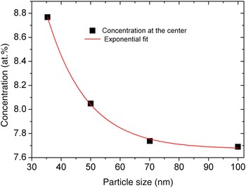
Concentration change at the center versus size of particles after 50 µs.

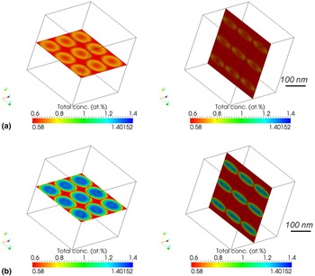
Concentration evolution of Li x C6 electrode particles along the xz- (left) and yz (right)-axes slices after (a) 2.5 s (top) and (b) 5 s (bottom), respectively. Simulation box size: 50·(∆x)3 with ∆x = 10 nm.

Influence of particle size
As recently reported in,[ Reference Malik, Burch, Bazant and Ceder 56 – Reference Kai, Kobayashi, Miyashiro, Oyama, Nishimura, Okubo and Yamada 59 ] the size of particles affects the kinetics of intercalation. Because the capacity of an electrode is a function of SOC, thickness of electrode and volume fraction of the active particles, the faster the kinetics of the battery, the better the performance.[ Reference Dua, Gupta, Zhang, Sastry and Shyy 60 – Reference Abraham, Liu, Chen, Hyung, Stoll, Elsen, MacLaren, Twesten, Haasch, Sammann, Petrov, Amine and Henriksen 64 ] A prior prediction of the size of active particles by theoretical simulation helps in the design of electrodes with higher performance to determine an appropriate size for active particles to get an electrode with superior performance. Now the question is which size range of active particles results in faster kinetics of intercalation for Li.
Particles with different sizes were considered. Flux of Li is proportional to the surface area of the active particles. If we reduce the size of the electrode particles, keeping the surface area of the particles constant, we can study the influence of the size on the kinetics. According to this phase field simulation result, the smaller particles show faster kinetics than the larger ones. Figure 9 shows how the kinetics of intercalation is faster for smaller particles. This could be due to the large number of surfaces created for diffusion. Larger number of surfaces means that Li ions have more probabilities of diffusing into these surfaces thereby increasing the rate of Li intercalation.
In a similar fashion, electrode particles composed of Li x C6 in an electrolyte solution of 1 mol/L LiPF6 salt solution is simulated. The input parameters used are shown in Table II. From Fig. 9, we can observe that more Li piles up near the vicinity of the interface between the particles and the electrolyte, thereby increasing the concentration of Li at the interface. One important aspect of this simulation is the simulation result along the xz- and yz-planes show different results. This is clearly shown in Fig. 9 where the slice along the yz-planes (ellipsoidal particles) show more Li intercalating near the tips of the ellipsoidal particles whereas slices along the xz-plane shows equal distribution of Li across the interface between the particles and electrolyte. This could be due to the high flux of Li across the higher curvature directions.
Conclusions
In this work, the finite interface dissipation phase field model has been applied to electrode-electrolyte interface modeling. We built a new bridge between electrochemistry and mesoscale simulations. This link was formulated by the current density, which can be measured by either impedance spectroscopy or by CV. With the help of the charge transfer resistance across the interface, it is possible to estimate electrochemical interface permeability. A detailed description of the interface permeability for an electrochemical interface is given. This approach will have a paramount importance in the understanding and modeling of the influence of coatings, passivation and heterogeneous catalysis as well as the SEI and other electrochemical properties upon charge and discharge of battery materials. Furthermore, future work shall lie on coupling synthesis methods (experimental) with (de)intercalation kinetics investigation, which is inevitable for predicting an optimized synthesis route for electrode particles that could give rise to high performance batteries. This will enhance the innovation of materials by integrated computation and experimental analysis.
Acknowledgments
The authors like to thank Dr. Ulrich Preiss for contributing to the model development and for useful discussions. We acknowledge financial support through the International Max Planck Institute for Surface and Interface Engineering of Materials (IMPRS-SurMat) and ICAMS and Addis Ababa University for supporting the preparation of this manuscript.