Structure and design

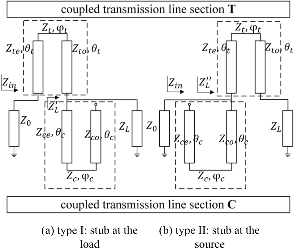
Figure 1 shows that the circuit structure of the proposed quad-band impedance transformer is simply composed of two sections of coupled line sections T and C, and section C is an open-circuit form. Section T is the coupled transmission line, and section C is the stubbed coupled line, respectively, in Figure 1(a) and Figure 1(b). The structures of two types are shown in Figure 1(a) and Figure 1(b).

Figure 1.

Structure of the proposed quad-band transformer. (a) Type I: stub at the load. (b) Type II: stub at the source.

As shown in Figure 1, the odd and even mode characteristic impedances of T and C coupled transmission lines are ${Z_{to}}$, ${Z_{te}}$, ${Z_{co}}$, and ${Z_{ce}}$ and the image impedance of T and C are ${Z_t}$, ${Z_c}$. The ${\varphi _t}$ and ${\varphi _c}$ are insert phases of the coupled transmission line sections T and C. With the equal electrical lengths ${\theta _t}$ and ${\theta _c}$ of the two modes, the odd and even modes, it is set to the same odd and even mode impedance ratio $\rho $ $\left( {\rho \gt 1} \right)$ for transmission lines according to Jones’ theory in Bai et al. [Reference Jones18], so we can give the following equations:

(1)\begin{equation}\begin{array}{*{20}{c}} {{Z_t} = \sqrt {{Z_{te}} \cdot {Z_{to}}} } \end{array}\end{equation}

(2)\begin{equation}\begin{array}{*{20}{c}} {{Z_c} = \sqrt {{Z_{ce}} \cdot {Z_{co}}} } \end{array}\end{equation}

(3)\begin{equation}\begin{array}{*{20}{c}} {\frac{{{Z_{te}}}}{{{Z_{to}}}} = \frac{{{Z_{ce}}}}{{{Z_{co}}}} = \rho } \end{array}\end{equation}

(4)\begin{equation}\begin{array}{*{20}{c}} {\cos {\varphi _t} = \frac{{\rho - {{\tan }^2}{\theta _t}}}{{\rho + {{\tan }^2}{\theta _t}}}} \end{array}\end{equation}

(5)\begin{equation}\begin{array}{*{20}{c}} {\cos {\varphi _c} = \frac{{\rho - {{\tan }^2}{\theta _c}}}{{\rho + {{\tan }^2}{\theta _c}}}} \end{array}\end{equation}

The ratio parameter of the impedance transformer between source impedance and load impedance is defined as follows.

(6)\begin{equation}\begin{array}{*{20}{c}} {K = \frac{{{Z_0}}}{{{Z_L}}} = \frac{{{Z_{in}}}}{{{Z_L}}}} \end{array}\end{equation}

Type I: coupled line shunted at the load

We can give the input impedance ${Z_{in}}$ of the two-section line according to the transmission line theory, as in the circuit structure shown in Figure 1(a).

(7)\begin{equation}\begin{array}{*{20}{c}} {{Z_{in}} = {Z_t}\frac{{Z_L^{\text{'}} + j{Z_t}\tan {\varphi _t}}}{{{Z_t} + jZ_L^{\text{'}}\tan {\varphi _t}}}} \end{array}\end{equation}

(8)\begin{equation}\begin{array}{*{20}{c}} {Z_L^{\text{'}} = \frac{{\frac{{{Z_c}}}{{j\tan {\varphi _c}}} \cdot {Z_L}}}{{\frac{{{Z_c}}}{{j\tan {\varphi _c}}} + {Z_L}}}} \end{array}\end{equation}

Substitute (8) into (7) and observe the real part and the imaginary part, respectively, we can get the following equations:

(9)\begin{equation}\begin{array}{*{20}{c}} {\left\{ {\begin{array}{*{20}{c}} {{Z_{in}}{Z_t}{Z_c} = {Z_t}{Z_c}{Z_L} - Z_t^2{Z_L}\tan {\varphi _c}\tan {\varphi _t}} \\ {j{Z_{in}}{Z_t}{Z_L}\tan {\varphi _c} + j{Z_{in}}{Z_c}{Z_L}\tan {\varphi _t} = jZ_t^2{Z_c}\tan {\varphi _t}} \end{array}} \right.} \end{array}\end{equation}

Equation (9) can be written as follows:

(10)\begin{equation}\begin{array}{*{20}{c}} {\left\{ {\begin{array}{*{20}{c}} {\tan {\varphi _c}\tan {\varphi _t} = \frac{{{Z_c}{Z_L} - {Z_{in}}{Z_c}}}{{{Z_t}{Z_L}}}} \\ {\frac{{\tan {\varphi _c}}}{{\tan {\varphi _t}}} = \frac{{Z_t^2{Z_c} - {Z_{in}}{Z_c}{Z_L}}}{{{Z_{in}}{Z_t}{Z_L}}}} \end{array}} \right.} \end{array}\end{equation}

Then, to simply the derivation process, let ${\theta _t} = {\theta _c} = \theta $, therefore ${\varphi _t} = {\varphi _c} = \varphi $, and we can rewrite (9) in the following form:

(11)\begin{equation}\begin{array}{*{20}{c}} {\left\{ {\begin{array}{*{20}{c}} {{{\tan }^2}\varphi = \frac{{{Z_c}{Z_L} - {Z_{in}}{Z_c}}}{{{Z_t}{Z_L}}}} \\ {1 = \frac{{Z_t^2{Z_c} - {Z_{in}}{Z_c}{Z_L}}}{{{Z_{in}}{Z_t}{Z_L}}}} \end{array}} \right.} \end{array}\end{equation}

Let $\alpha \equiv {\tan ^2}\varphi $. By solving (11), the following equation is derived:

(12)\begin{equation}\begin{array}{*{20}{c}} {\left\{ {\begin{array}{*{20}{c}} {{Z_t} = \sqrt {{Z_{in}}{Z_L} - \frac{{{Z_{in}}\left( {{Z_{in}} - {Z_L}} \right)}}{\alpha }} } \\ {{Z_c} = \frac{{\alpha {Z_t}{Z_L}}}{{{Z_L} - {Z_{in}}}}} \end{array}} \right.} \end{array}\end{equation}

Together with (4), (5), and (11), we can obtain:

(13)\begin{equation}\begin{array}{*{20}{c}} {\left\{ {\begin{array}{*{20}{c}} {\alpha = {{\tan }^2}\varphi } \\ {{{\tan }^2}\theta = \rho \frac{{1 - \cos \varphi }}{{1 + \cos \varphi }} = \rho {{\tan }^2}\frac{\varphi }{2}} \end{array}} \right.} \end{array}\end{equation}

We can obtain an expression about $\theta $ by solving the equations above.

(14)\begin{equation}\begin{array}{*{20}{c}} {\theta = m\pi \pm \arctan \left( {\sqrt \rho \tan \frac{{n\pi \pm \arctan \sqrt \alpha }}{2}} \right)} \end{array}\end{equation}

Both $m$ and $n$ are arbitrary integers, so we can get four unrelated solutions for $\theta $ from (14). Since $\theta \gt 0$ and a small size impedance transformer is what we want to realize. Therefore, (+) sign is chosen in (14) when $m = n = 0$ and (−) sign is chosen in (14) when $m = n = 1$. Considering the generality, we assume that ${f_1} \lt {f_2} \lt {f_3} \lt {f_4}$, and we can obtain the four fundamental solutions about $\theta $ from (14).

(15)\begin{equation}\begin{array}{*{20}{c}} {\left\{ {\begin{array}{*{20}{c}} {{\theta _1} = \arctan (\sqrt \rho \tan \frac{{\arctan \sqrt \alpha }}{2})} \\ {{\theta _2} = \arctan (\sqrt \rho \tan \frac{{\pi - \arctan \sqrt \alpha }}{2})} \\ {{\theta _3} = \pi - \arctan (\sqrt \rho \tan \frac{{\pi - \arctan \sqrt \alpha }}{2})} \\ {{\theta _4} = \pi - \arctan (\sqrt \rho \tan \frac{{\arctan \sqrt \alpha }}{2})} \end{array}} \right.} \end{array}\end{equation}

This means the impedance transformer can perfectly match impedance at four different frequencies. Furthermore, assuming $0 \lt {\theta _1} \lt {\theta _2} \lt {\theta _3} \lt {\theta _4} \lt \pi $. The relationships between ${\theta _1}$, ${\theta _2}$ ${\theta _3}$ and ${\theta _4}$ could be obtained from (15) as follows:

(16)\begin{equation}\begin{array}{*{20}{c}} {\tan {\theta _1}\tan {\theta _2} = \sqrt \rho \tan \frac{{\arctan \sqrt \alpha }}{2}\sqrt \rho \tan \frac{{\pi - \arctan \sqrt \alpha }}{2} = \rho } \end{array}\end{equation}

(17)\begin{equation}\begin{array}{*{20}{c}} {\frac{{\tan {\theta _1}}}{{\tan {\theta _2}}} = {{\tan }^2}\left( {\frac{{\arctan \sqrt \alpha }}{2}} \right)} \end{array}\end{equation}

(18)\begin{equation}\begin{array}{*{20}{c}} {{\theta _1} + {\theta _4} = {\theta _2} + {\theta _3} = \pi } \end{array}\end{equation}

According to the electrical length definition, we know

(19)\begin{equation}\begin{array}{*{20}{c}} {\theta = \beta l = \frac{{2\pi f}}{c}l} \end{array}\end{equation}

The $l$ is the physical length of the single coupled line, and the $c$ is the velocity of light. If we fix the physical length of the single coupled line and determine it as ${l_0}$, we will obtain

(20)\begin{equation}\begin{array}{*{20}{c}} {{\theta _i} = {\beta _i}{l_0} = \frac{{2\pi {f_i}}}{c}{l_0}\,\,\,\,\left( {i = 1,2,3,4} \right)} \end{array}\end{equation}

A frequency variable ${f_0}$ can be given from (18) and (20) as follows:

(21)\begin{equation}\begin{array}{*{20}{c}} {{f_0} \equiv \frac{{{f_1} + {f_4}}}{2} = \frac{{{f_2} + {f_3}}}{2} = \frac{c}{{4{l_0}}}} \end{array}\end{equation}

If frequencies ${f_1}$, ${f_2}$, ${f_3}$ are given, the physical length of a single coupled line section ${l_0}$ can be calculated from (21) and we can write it as follows:

(22)\begin{equation}\begin{array}{*{20}{c}} {{l_0} = \frac{c}{{4{f_0}}}} \end{array}\end{equation}

Electrical lengths ${\theta _i}$, $\rho $, and $\alpha $ can be calculated by

(23)\begin{equation}\begin{array}{*{20}{c}} {{\theta _i} = {\beta _i}{l_0} = \frac{{\pi {f_i}}}{{2{f_0}}}} \end{array}\end{equation}

(24)\begin{equation}\begin{array}{*{20}{c}} {\rho = \tan \left( {\frac{{\pi {f_1}}}{{2{f_0}}}} \right)\tan \left( {\frac{{\pi {f_2}}}{{2{f_0}}}} \right)} \end{array}\end{equation}

(25)\begin{equation}\begin{array}{*{20}{c}} {\alpha = {{\tan }^2}\left( {2\arctan \sqrt {\frac{{\tan \left( {\frac{{\pi {f_1}}}{{2{f_0}}}} \right)}}{{\tan \left( {\frac{{\pi {f_2}}}{{2{f_0}}}} \right)}}} } \right)} \end{array}\end{equation}

So far, the deduction of the design equations for the designed impedance transformer of type I has been completed.

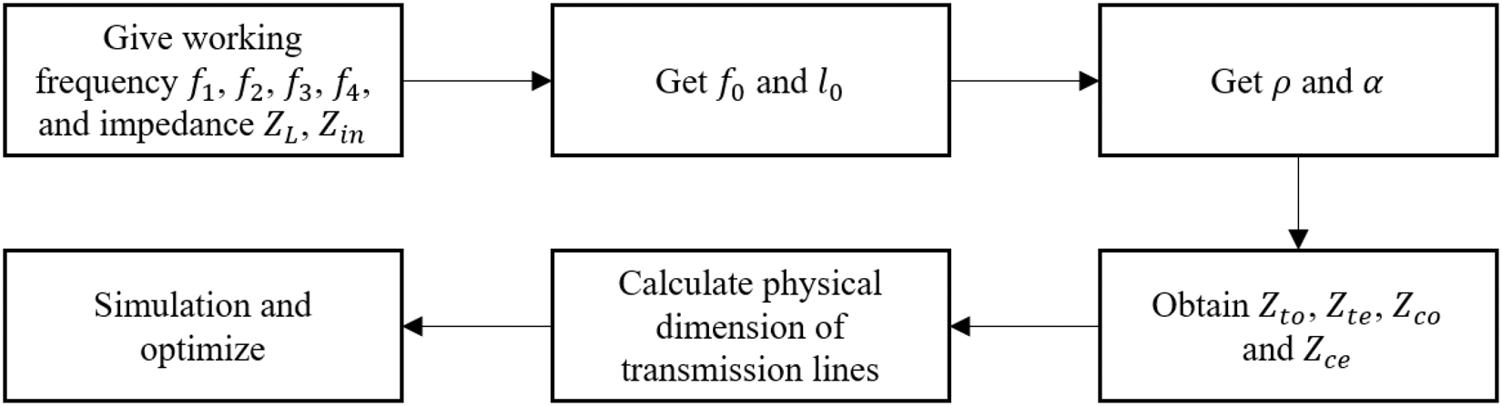
Design process is shown in Figure 2. If we give ${f_1}$, ${f_2}$, ${f_3}$ and ${f_4}$ firstly, ${f_0}$ and ${l_0}$ can be calculated by (21) and (22). Second, $\rho $ and $\alpha $ can be calculated by (24) and (25). Third, we can know the image impedance ${Z_t}$ and ${Z_c}$ from (12). Then, according to (1), (2) and (3), the odd and even mode characteristic impedance ${Z_{to}}$, ${Z_{te}}$, ${Z_{co}}$, and ${Z_{ce}}$ can be obtained. Eventually, the basic parameters of the Quad-band impedance transformer can be determined.

Figure 2.

Design process.

Type II: coupled line shunted at the source

As type II shown in Figure 1(b), with the stubbed coupled line section shunted at the source, the equations can be derived similarly. According to the transmission line theory, we can also give the input Impedance ${Z_{in}}$ of two-section line.

(26)\begin{equation}\begin{array}{*{20}{c}} {{Z_{in}} = \frac{{\frac{{{Z_c}}}{{j\tan {\varphi _c}}}{Z_L}^{{\text{''}}}}}{{\frac{{{Z_c}}}{{j\tan {\varphi _c}}} + {Z_L}^{{\text{''}}}}}} \end{array}\end{equation}

(27)\begin{equation}\begin{array}{*{20}{c}} {{Z_L}^{{\text{''}}} = {Z_t}\frac{{{Z_L} + j{Z_t}\tan {\varphi _t}}}{{{Z_t} + j{Z_L}\tan {\varphi _t}}}} \end{array}\end{equation}

Similarly, the solutions are obtained by solving the equations as follows:

(28)\begin{equation}\begin{array}{*{20}{c}} {\left\{ {\begin{array}{*{20}{c}} {{Z_t} = \sqrt {{Z_{in}}{Z_L} - \frac{{{Z_L}\left( {{Z_L} - {Z_{in}}} \right)}}{\alpha }} } \\ {{Z_c} = \frac{{\alpha {Z_t}{Z_{in}}}}{{{Z_{in}} - {Z_L}}}} \end{array}} \right.} \end{array}\end{equation}

These two structures mirror each other, and the design process is the same as described in the case that the stubbed coupled line section C is shunted at the load end. To match real impedance load, it can be seen that in (12) that ${Z_0}$ should be smaller than ${Z_L}$, however in (28), ${Z_0}$ should be larger than ${Z_L}$, which means that cases change with structures changing.

Analysis and simulations

The solutions mentioned above are elementary in nature and are in open-circuit form. However, not all frequencies are ideal for realizing the application, so we must consider the available ranges of frequency ratios. Thus, to describe the relationship between different frequencies better, we let ${f_2} = p{f_1}$, ${f_3} = q{f_2}$,so ${f_3} = pq{f_1}$, where $p$, $q$ is the frequency-ratio and $1 \lt p \lt pq$. So we can rewrite (24) as follows by replacing frequencies.

(29)\begin{equation}\begin{array}{*{20}{c}} {\rho = \tan \frac{\pi }{{p\left( {q + 1} \right)}}\tan \frac{{p\pi }}{{p\left( {q + 1} \right)}}} \end{array}\end{equation}

Then, we obtain by (29) since $\rho \gt 1$.

(30)\begin{equation}\begin{array}{*{20}{c}} {\frac{{\sin \frac{\pi }{{p\left( {q + 1} \right)}}\sin \frac{{p\pi }}{{p\left( {q + 1} \right)}}}}{{\cos \frac{\pi }{{p\left( {q + 1} \right)}}\cos \frac{{p\pi }}{{p\left( {q + 1} \right)}}}} \gt 1} \end{array}\end{equation}

We can get $\cos \frac{\pi }{{p\left( {q + 1} \right)}} \gt 0$ and $\cos \frac{{p\pi }}{{p\left( {q + 1} \right)}} \gt 0$ since $1 \lt p \lt pq$. Equation (30) can be derived as follows after rearrangement and using trigonometric formula.

(31)\begin{equation}\begin{array}{*{20}{c}} {\cos \frac{{\left( {p + 1} \right)\pi }}{{p\left( {q + 1} \right)}} \lt 0} \end{array}\end{equation}

The solution of Equation (31) is

(32)\begin{equation}\begin{array}{*{20}{c}} {\frac{{2 - p\left( {4n + 1} \right)}}{{p\left( {4n + 3} \right)}} \lt q \lt \frac{{2 + p\left( {1 - 4n} \right)}}{{p\left( {4n + 1} \right)}}} \end{array}\end{equation}

Where $n$ is an arbitrary integer. With $1 \lt p \lt pq$, (32) can be simplified as

(33)\begin{equation}\begin{array}{*{20}{c}} {1 \lt q \lt \frac{{2 + p}}{p}} \end{array}\end{equation}

Multiply by $p{f_1}$, we obtain

(34)\begin{equation}\begin{array}{*{20}{c}} {{f_1} \lt {f_2} \lt {f_3} \lt 2{f_1} + {f_2}} \end{array}\end{equation}

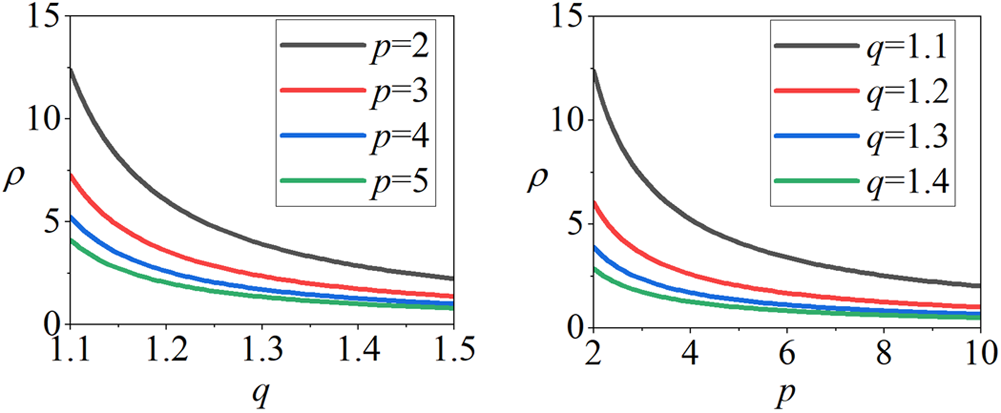
Figure 3 shows the relationships between the impedance ratio $\rho $ and frequency ratio $p$ and $q$, we can obtain this conclusion that ratio $\rho $ is reducing with the increase of $p$ and $q$, which means ratio $\rho $ is reducing with the increase of designed frequency ratio.

Figure 3.

Relationship between $\rho $, frequency-ratios $p$ and $q$.

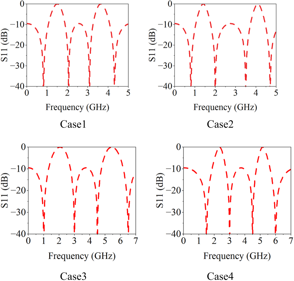
We give some examples under the condition that $K = 0.5$, as listed in Table 1. Figure 4 shows the theoretic $\left| {{S_{11}}} \right|$ under the condition with fixed ${f_1}$, ${f_2}$ and $p = 2.5$ and fixed ${f_2}$, ${f_3}$ and $q = 1.5$. It can be seen that the $\left| {{S_{11}}} \right|$ is well-matched with designed frequencies.

Figure 4.

Theoretic $\left| {{S_{11}}} \right|$ under the conditions from Table 1.

Table 1.

Simulations on condition $K = 0.5$ ( $p = 2.5$ or $q = 1.5$)

Experiment results

Considering non-TEM behavior in microstrip realization in the application, a stepped impedance coupled line is used in model building [Reference Schiek and Kohler19].To verify the matching at the four frequency points, we choose F4BM-2 ( $tan{ }\delta \leqslant 0.0007$) with a relative permittivity of 2.55 and the thickness $h$ of $0.762mm$ as the dielectric substrate to fabricate a quad-band impedance transformer at 0.7/2.4/3.6/5.3 GHz, which could be applied to Power Divider, Coupler, Antenna, Filter, Mixer Power Amplifier, and LNA. 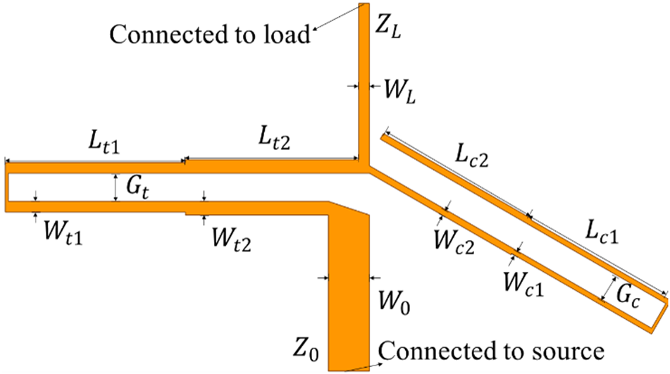Here we set ${Z_0} = 50{\Omega }$ and ${Z_L} = 100{\Omega }$. The model of the designed impedance transformer with the dimension being labeled and the photo of it are shown in Figure 5 and Figure 6. The numerical results are calculated by MATLAB R2022b, and we obtain the simulated results by Advanced Design Systems (ADS).

Figure 5.

The model of the designed impedance transformer with the dimension being labeled.

Figure 6.

The photo of the designed impedance transformer.

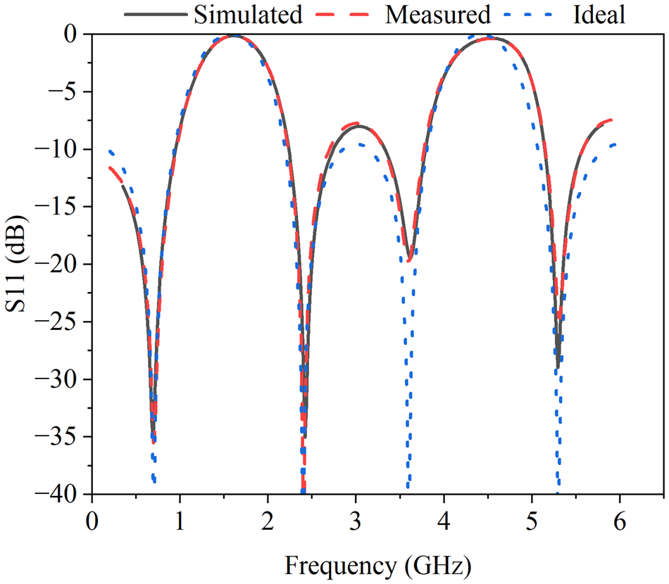
By the equations above, we can calculate that ${Z_{te}} = 102.19{\Omega }$, ${Z_{to}} = 86.50{\Omega }$, ${Z_{ce}} = 133.09{\Omega }$, ${Z_{co}} = 112.66{\Omega }$. Then, we optimize the result through simulation and final dimensions are listed in Table 2. It is shown in Figure 7 about the measured results of S-parameters for the magnitude of $\left| {{S_{11}}} \right|$ obtained from the Agilent N5230A network analyzer and the simulated results. We can directly see that the measured results of the $\left| {{S_{11}}} \right|$ are about −35.5 dB at 0.7 GHz, −35.8 dB at 2.4 GHz, −19.7 dB at 3.6 GHz, and −24.5 dB at 5.3 GHz. The two curves fit very well in Figure 7, which means that the measured results are in good agreement with the simulated results at four designed frequencies. The designed impedance is practicable. Compared with the result in Chongcheawchamnan et al. [Reference Wang, Zhang, Xu, Bai, Liu and Shi17], simulated and measured curves fit better in this paper. There are some small differences between measured and simulated results, these could be caused by material purity, manufacturing limitation, coaxial line connector welding, and measurement accuracy.

Figure 7.

Simulated and measured $\left| {{S_{11}}} \right|$ results of the designed impedance transformer.

Table 2.

Optimized dimensions (unit millimeter)