1. Introduction
The concept of granular fluid can be used in order to model the flow of a large quantity of solid particles (see Andreotti, Forterre & Pouliquen Reference Andreotti, Forterre and Pouliquen2013). In dense regimes, the particles tend to stay in contact with each other and a macroscopic behaviour can be observed. This kind of flow can be found in many geophysical contexts, for which, in the presence of topography, the flow is driven by gravity. Two examples are landslides or dry snow avalanches. Modelling the flow of granular media with a good accuracy is thus of crucial importance in a large range of applications.
Granular flows exhibit complex behaviours that are distinct from more ‘classical’ flows. In the context of flow down an inclined plane, a way to model these particular aspects is to use an adequate friction law. Granular friction laws were first introduced at the depth-averaged level. For numerical applications, depth-averaged models present the advantage of a reduced computation time. A first attempt to model granular flows specifically was proposed in 1989 by Savage & Hutter (Reference Savage and Hutter1989) using a solid friction law. This model has some similarities with older models of dense snow avalanches, which also added an empirical fluid friction term. The approach of Savage & Hutter (Reference Savage and Hutter1989) was extended to two dimensions and to complex topographies and applied to many cases of geophysical flows (e.g. Denlinger & Iverson Reference Denlinger and Iverson2001; Pitman et al. Reference Pitman, Nichita, Patra, Bauer, Sheridan and Bursik2003; Pudasaini & Hutter Reference Pudasaini and Hutter2003; Bouchut & Westdickenberg Reference Bouchut and Westdickenberg2004; Denlinger & Iverson Reference Denlinger and Iverson2004; Mangeney-Castelnau et al. Reference Mangeney-Castelnau, Bouchut, Vilotte, Lajeunesse, Aubertin and Pirulli2005; Larrieu, Staron & Hinch Reference Larrieu, Staron and Hinch2006; Peruzzetto et al. Reference Peruzzetto, Komorowski, Le Friant, Rosas-Carbajal, Mangeney and Legendre2019).
As it became clear that granular flows could not always be described by a solid friction law, a more elaborate friction law was proposed. An empirical approach was used by Pouliquen (Reference Pouliquen1999) to derive a friction law based on experimental observations, still at the depth-averaged level. This law was refined by Pouliquen & Forterre (Reference Pouliquen and Forterre2002) who also proposed a non-monotonic law for the friction coefficient, distinguishing between dynamic and static regimes, as well as an intermediate regime taken into account by an extrapolation function. Contrary to the assumption of constant solid friction, these friction laws are compatible with the existence of steady uniform flows over a range of inclination angles for granular flows down a rough incline. The non-monotonic friction law is able to capture frictional hysteresis.
A specific granular rheology was then presented (GDR MiDi 2004), in which the friction coefficient
 $\mu$
is a function of a dimensionless parameter
 $I$
, called the inertial number. The inertial number is interpreted as a ratio between two time scales related to the microscopic structure of the granular media (GDR MiDi 2004). This
 $\mu (I)$
rheology was then generalised into a constitutive law at the bulk level, for two-dimensional (2-D) flows (GDR MiDi 2004; Jop, Forterre & Pouliquen Reference Jop, Forterre and Pouliquen2005; Pouliquen et al. Reference Pouliquen, Cassar, Forterre, Jop and Nicolas2005) and three-dimensional flows (Forterre Reference Forterre2006; Jop, Forterre & Pouliquen Reference Jop, Forterre and Pouliquen2006). The basal friction law of the model of Pouliquen & Forterre (Reference Pouliquen and Forterre2002) can be reinterpreted in the context of the
 $\mu (I)$
rheology (Andreotti et al. Reference Andreotti, Forterre and Pouliquen2013). Extensions of the depth-averaged model to the 2-D case on complex topography with applications to geophysical flows were proposed with the friction law of Pouliquen (Reference Pouliquen1999) (Mangeney-Castelnau et al. Reference Mangeney-Castelnau, Vilotte, Bristeau, Perthame, Bouchut, Simeoni and Yerneni2003) or with the non-monotonic friction law of Pouliquen & Forterre (Reference Pouliquen and Forterre2002) (Mangeney et al. Reference Mangeney, Bouchut, Thomas, Vilotte and Bristeau2007).
Roll waves for dense granular flows were experimentally observed by Forterre & Pouliquen (Reference Forterre and Pouliquen2003), who also measured the phase velocity and the spatial growth rate. This instability occurs above a critical Froude number and disappears above a cutoff frequency. This cutoff frequency does not appear in models that only take into account friction effects. By adding a diffusive term to the depth-averaged model, Forterre (Reference Forterre2006) and Gray & Edwards (Reference Gray and Edwards2014) derived models capable of predicting the existence of this cutoff frequency in agreement with the experimental data of Forterre & Pouliquen (Reference Forterre and Pouliquen2003). The spatial growth rate is also accurately predicted.
The diffusive model of Gray & Edwards (Reference Gray and Edwards2014) was used with the friction coefficient of Pouliquen & Forterre (Reference Pouliquen and Forterre2002) in the dynamic regime to model granular roll waves (Razis et al. Reference Razis, Edwards, Gray and van der Weele2014) and dense granular avalanches (Baker et al. Reference Baker, Barker and Gray2016a ), as well as with the non-monotonic friction law (Pouliquen & Forterre Reference Pouliquen and Forterre2002; Edwards et al. Reference Edwards, Viroulet, Kokelaar and Gray2017) to model erosion--deposition waves and the formation of levees (Edwards & Gray Reference Edwards and Gray2015; Edwards et al. Reference Edwards, Viroulet, Kokelaar and Gray2017; Rocha, Johnson & Gray Reference Rocha, Johnson and Gray2019). The importance of the diffusive term in the depth-averaged model was highlighted by Baker et al. (Reference Baker, Barker and Gray2016a ) and Rocha et al. (Reference Rocha, Johnson and Gray2019) and also by Baker et al. (Reference Baker, Johnson and Gray2016b ) for segregation-induced finger formation in granular flows.
Despite the many successes of the
 $\mu (I)$
rheology in describing granular flows, it has been shown by Barker et al. (Reference Barker, Schaeffer, Bohórquez and Gray2015) that this rheology is well-posed for intermediate inertial numbers, but can be ill-posed for low or high inertial numbers. This ill-posed behaviour is due to a short-wavelength instability with an infinite growth rate in the infinite wavenumber limit. Modifications to the
 $\mu (I)$
rheology involving compressibility were proposed by Barker et al. (Reference Barker, Schaeffer, Shearer and Gray2017), Heyman et al. (Reference Heyman, Delannay, Tabuteau and Valance2017) and Schaeffer et al. (Reference Schaeffer, Barker, Tsuji, Gremaud, Shearer and Gray2019) to solve this problem (see also the remarks of Goddard & Lee Reference Goddard and Lee2018). Further work on this subject is provided by Goddard & Lee (Reference Goddard and Lee2017).
In the case of thin layers, depth-averaged models can be derived by introducing a small parameter
 $\varepsilon$
, which is a ratio between a vertical and a horizontal length scale, thus defining a shallow flow, and by using an asymptotic method with a systematic expansion of the variables in the governing equations as power series of the parameter
 $\varepsilon$
. The leading order, or zeroth order in
 $\varepsilon$
, governs the steady uniform flows. To model flows that are not stationary and uniform, it is important to ensure model consistency up to the first order in
 $\varepsilon$
. The definition of the consistency of a model (see Richard et al. Reference Richard, Gisclon, Ruyer-Quil and Vila2019) is relative to a set of hypotheses concerning the order of magnitude of the dimensionless numbers of the problem. In the case of granular flows down an incline, these numbers are the Froude number and the slope. Both are of
 $O(1)$
with respect to the small parameter
 $\varepsilon$
, since neither is particularly small in the case of granular flows studied in the laboratory or encountered in nature. A model can always be written in such a way that the dominant terms are of
 $O(1)$
. A model written in this way is said to be consistent of order
 $n$
if, after substituting the model variables with their asymptotic expansions, all the terms disappear except for an
 $O(\varepsilon ^{n+1})$
remainder.
Model consistency means that the approximation used to derive the model is consistent. In practice, only the first-order consistency is really important. Therefore, the consistency implies that no term of first order is neglected. From a more physical point of view, the relations obtained for steady uniform flows are not exactly valid for variable flows. Consistency allows us to calculate the first-order corrections that appear for variable flows. These corrections result in terms of order 1 in the model. One of the consequences of writing an inconsistent model is that the stability threshold of the Kapitza instability predicted by the model differs from the threshold corresponding to the rheology in the long-wave limit. Consistency, on the other hand, ensures that the long-wave instability threshold predicted by the model and by rheology coincides exactly.
This asymptotic method was already used to derive consistent depth-averaged models for Newtonian fluids (e.g. Ruyer-Quil & Manneville Reference Ruyer-Quil and Manneville2000; Richard, Ruyer-Quil & Vila Reference Richard, Ruyer-Quil and Vila2016), power-law fluids (Noble & Vila Reference Noble and Vila2013) and viscoplastic flows (Denisenko, Richard & Chambon Reference Denisenko, Richard and Chambon2023), but no depth-averaged model of dense granular flow consistent with the incompressible
 $\mu (I)$
rheology has been derived. As a consequence, the instability threshold of steady uniform flows of the existing models (e.g. Forterre & Pouliquen Reference Forterre and Pouliquen2003; Gray & Edwards Reference Gray and Edwards2014) is different from the theoretical one that was calculated by Forterre (Reference Forterre2006) with the
 $\mu (I)$
rheology in the long-wave limit, because the bottom friction has been estimated from steady uniform flow relations, so that the first-order correction in
 $\varepsilon$
has been neglected.
Another inconsistency is due to the treatment of the depth-averaged value
 $\langle u^2 \rangle$
of the square of the velocity
 $u$
in the momentum flux. Since this flux term is already of first order in
 $\varepsilon$
, it can be estimated, for a first-order model, from the zero-order expression of
 $u$
(steady uniform flows relations). If a no-slip condition is assumed at the bottom, the flow is strongly sheared and shear effects cannot be consistently neglected in the depth-averaged model. A first approach that has been used by Forterre & Pouliquen (Reference Forterre and Pouliquen2003) and Gray & Edwards (Reference Gray and Edwards2014) is to introduce a parameter
 $\alpha$
, called the shape factor, which depends on the velocity profile, writing
 $\langle u^2 \rangle = \alpha \langle u \rangle ^2$
. For a sheared flow, the shape factor is always greater than 1. In the case of steady and uniform granular flows, the velocity profile is a Bagnold profile (Andreotti et al. Reference Andreotti, Forterre and Pouliquen2013) and the shape factor is equal to
 $5/4$
. If
 $\alpha =5/4$
, the model strongly overestimates the instability threshold of the Kapitza instability (Forterre Reference Forterre2006). The agreement is better if a constant velocity profile is assumed (
 $\alpha =1$
). The inconsistency of existing models therefore leads either to very significant deviations from predictions of the
 $\mu (I)$
rheology if the Bagnold profile is taken into account, or, paradoxically, to more reasonable (but nonetheless significant) deviations if the velocity profile of equilibrium granular flows is not taken into account. This shortcoming is directly attributable to the inconsistency of the derivation. A consistent model exactly predicts the instability threshold corresponding to the rheology while taking into account a Bagnold velocity profile for a steady uniform flow. Consistency at the first order of accuracy is sufficient to obtain these properties. Second-order terms are only useful to include diffusive effects in the model since diffusion is absent in a first-order model.
An additional difficulty is that the mathematical structure of the model is not satisfactory if
 $\alpha \neq 1$
, because there is no energy balance equation for the system. The compatibility with an energy balance equation implies that
 $\alpha =1$
. The proof of Richard & Gavrilyuk (Reference Richard and Gavrilyuk2012, Appendix A) can be used straightforwardly for the model of Gray & Edwards (Reference Gray and Edwards2014). It is usually better to take
 $\alpha = 1$
, thus loosing the consistency for a sheared flow.
A strategy for taking into account a depth-varying velocity profile in a depth-averaged model in a consistent and well-posed way is to take the shear into account with an additional depth-averaged variable
 $\langle (u-\langle u \rangle )^2 \rangle /h^2$
(where
 $h$
is the depth and
 $\langle \cdot \rangle$
the depth-averaging operator), called enstrophy because it is related to the square of the vorticity. This approach was initiated by Teshukov (Reference Teshukov2007) and developed by Richard & Gavrilyuk (Reference Richard and Gavrilyuk2012) and Richard et al. (Reference Richard, Ruyer-Quil and Vila2016) in particular. The depth-averaged model is thus a system of three equations which admits, by construction, an energy balance equation. The variables are the depth of the flow, the depth-averaged velocity, which are the usual variables for shallow-water equations, and the enstrophy. In one dimension and in the absence of diffusion, the obtained model is a hyperbolic system of conservation laws analogous to the compressible Euler equations. This enables us to use well-known reliable and stable numerical schemes. This approach is quite general and has been used to derive depth-averaged models in various contexts; see, for instance, Richard et al. (Reference Richard, Ruyer-Quil and Vila2016), Denisenko et al. (Reference Denisenko, Richard and Chambon2023) and Richard (Reference Richard2024).
The motivation of this work is to derive a depth-averaged, first-order consistent, well-posed model for granular flows down an inclined plane described by the standard
 $\mu (I)$
rheology, while taking into account a Bagnold velocity profile for steady uniform flows. The model must admit exactly an energy balance equation, both for physical and numerical reasons, since the stability of a numerical scheme implies preserving the energy balance in a discrete framework. Another advantage of the consistency of the derivation is the possibility of reconstructing the depth profile of velocity, from the values of the depth-averaged quantities calculated by the model. This type of reconstruction has been obtained in the case of turbulent open-channel flows (Richard, Couderc & Vila Reference Richard, Couderc and Vila2023) and for viscoplastic yield-stress fluids (Denisenko et al. Reference Denisenko, Richard and Chambon2023).
The paper is organised as follows. In § 2 we present the equations that govern the motion of the granular medium, as well as their dimensionless form in the long-wave limit. In § 3 we derive explicitly the asymptotic expansions at orders 0 and 1 in
 $\varepsilon$
. In § 4, the depth-averaged model is derived. The model is analysed in § 5 and is compared with experimental data of Forterre & Pouliquen (Reference Forterre and Pouliquen2003). An extended version of the model, that takes into account diffusive effects, is given in § 5.4. A numerical resolution in the case of granular roll waves is presented in § 5.6. The reconstruction of the velocity profile is obtained in § 5.1 and an example is given in § 5.6. The limitations of the model are explained in § 6.
2. Governing equations
2.1. Constitutive equations
We study the flow of a granular fluid, which is described by its density
 $\rho$
and its velocity
 $\boldsymbol {v}$
. We assume that the fluid is made of solid particles. Hence, the density is proportional to
 $\phi$
the volume fraction of the beads and is written as
 \begin{equation} \rho = \rho _p \phi , \end{equation}
where the constant
 $\rho _p$
is the density of the beads. We also suppose that the volume fraction
 $\phi$
is constant, which implies that the flow is incompressible. We assume that the fluid is flowing down an inclined plane that makes an angle
 $\theta$
with the horizontal. The motion of the fluid is described by the mass and momentum balance equations, which read in the incompressible case with constant density as
 \begin{equation} \begin{aligned} \frac {\partial \rho \boldsymbol {v}}{\partial t}+\mathbf {div}\left (\rho \boldsymbol {v}\otimes \boldsymbol {v}\right )&= \mathbf {div}\,\boldsymbol {\sigma }+\rho \boldsymbol {g},\\ \mathrm {div}\,\boldsymbol {v}&=0, \\ \phi &=\phi _c\,\, \mathrm {constant}. \end{aligned} \end{equation}
The second-order tensor
 $\boldsymbol \sigma$
is called the Cauchy stress tensor and can be written as
 \begin{equation} {\boldsymbol {\sigma }} = -p {\boldsymbol {I_d}} +{\boldsymbol {\tau }}, \end{equation}
where
 $\boldsymbol{I_d}$
is the identity tensor. The quantity
 $p$
is the pressure and
 $\boldsymbol {\tau }$
is the deviatoric stress tensor. It is given by the constitutive law
 \begin{equation} \boldsymbol {\tau } = \eta _e \boldsymbol {\dot {\gamma }}, \end{equation}
where
 \begin{equation} \boldsymbol {\dot {\gamma }}=\mathbf {grad}\,\boldsymbol {v}+\left (\mathbf {grad}\, \boldsymbol {v}\right )^{\mathrm {T}} \end{equation}
is the strain-rate tensor and
 $\eta _e$
is an effective viscosity. In the isotropic case,
 $\eta _e$
is a scalar. In order to define the effective viscosity, we introduce the inertial number
 $I$
, which is a dimensionless parameter given by the relation (GDR MiDi 2004)
 \begin{equation} I=\frac {|\boldsymbol {\dot {\gamma }}|d}{\sqrt {p/\rho _p}\,}. \end{equation}
The quantity
 $d$
is the diameter of a bead, and
 $|\boldsymbol {\dot {\gamma }}|$
is the norm of the second-order tensor
 $\boldsymbol {\dot {\gamma }}$
, defined by
 \begin{equation} |\boldsymbol {\dot {\gamma }}|=\sqrt {\frac {\boldsymbol {\dot {\gamma } : \dot {\gamma }}}{2}}. \end{equation}
We also introduce the friction coefficient
 $\mu (I)$
, which depends only on
 $I$
. The dependence is experimentally determined with three constants
 $\mu _1$
,
 $\mu _2$
and
 $I_m$
as (Jop et al. Reference Jop, Forterre and Pouliquen2006)
 \begin{equation} \mu (I)=\mu _1+\frac {\mu _2-\mu _1}{1+I_m/I}. \end{equation}
The two constants
 $\mu _1$
and
 $\mu _2$
are limit cases: the value
 $\mu _2$
is the maximal value of
 $\mu (I)$
, obtained when
 $I \to \infty$
, the value
 $\mu _1$
is the minimal value, obtained when
 $I=0$
, and the granular fluid only flows when
 $|\tau |\gt \mu _1 p$
. The existence of a maximum value for the friction coefficient is debated (see Holyoake & McElwaine Reference Holyoake and McElwaine2012; Barker & Gray Reference Barker and Gray2017), but only the standard
 $\mu (I)$
rheology will be considered in this paper. Note that this relation can be inverted to write
 \begin{equation} I=I_m\frac {\mu -\mu _1}{\mu _2-\mu }. \end{equation}
The expression of the effective viscosity is then
 \begin{equation} \eta _e=\mu (I)\frac {p}{|\boldsymbol {\dot {\gamma }}|}. \end{equation}
We denote by
 $z$
the coordinate in the direction normal to the inclined plane and by
 $x$
the coordinate in the direction parallel to the inclined plane (see figure 1). The components of the velocity
 $\boldsymbol {v}$
are
 $u$
and
 $w$
in the
 $x$
and
 $z$
directions, respectively.
Definition sketch.

The system (2.2) admits an energy balance equation. The mechanical energy density
 $E$
of the fluid is equal to the sum of the kinetic energy density and the gravitational potential energy density:
 \begin{equation} E=\frac {1}{2} \rho |\boldsymbol {v}|^2- \rho g x\sin \theta + \rho g z\cos \theta . \end{equation}
The energy balance equation is then
 \begin{equation} \frac {\partial E}{\partial t}+\mathrm {div}\left ( E\boldsymbol {v}\right )=\mathrm {div}\,\left (\boldsymbol {\sigma \cdot v}\right )-\frac {\boldsymbol {\sigma : \dot {\gamma }}}{2}. \end{equation}
Using the incompressibility condition, (2.12) can also be written as
 \begin{equation} \frac {\partial E}{\partial t} +\mathrm {div}\left [\left ( E+p\right )\boldsymbol {v}\right ]=\mathrm {div}\,\left (\boldsymbol {\tau \cdot v}\right )-\frac {\boldsymbol {\tau : \dot {\gamma }}}{2}. \end{equation}
The granular fluid is assumed to be delimited downwards by the inclined plane at
 $z=0$
, and a free surface upwards at
 $z=h$
. The field
 $h$
is a function of
 $(t,x)$
. For any field
 $f$
depending on the variable
 $z$
, we write
 $f(0):=f|_{z=0}$
and
 $f(h):=f|_{z=h}$
. We denote by
 $\boldsymbol {n}(t,x)$
the unit vector normal to the free surface and pointing outward the flow. It is given by
 \begin{equation} \boldsymbol {n}=\frac {1}{\sqrt {1+|\partial h / \partial x|^2}}\left (-\frac {\partial h}{\partial x},1\right )^{\mathrm {T}}. \end{equation}
We can now define the boundary conditions satisfied by the velocity:
-
(i) At
 $z=0$
, we assume a non-penetration condition given by(2.15)as well as a no-slip condition given by
\begin{equation} w(0)=0, \end{equation}
(2.16)
\begin{equation} u(0)=0. \end{equation}
-
(ii) At
$z=h$
, the velocity drives the evolution of the free surface via the kinematic boundary condition(2.17)
\begin{equation} \frac {\partial h}{\partial t}+u(h)\frac {\partial h}{\partial x} =w(h). \end{equation}


The dynamic boundary condition states that the normal stresses are continuous across the free surface. The normal stress above the free surface is given by the atmospheric pressure
 $p_{atm}$
. Without loss of generality, this constant can be taken equal to zero. This leads to the equation
 \begin{equation} \boldsymbol {\sigma }(h) \boldsymbol {\cdot } \boldsymbol {n}=0, \end{equation}
which expands as
 \begin{equation} \qquad\qquad\qquad\qquad\qquad\, \left\{\begin{array} {l@{\kern80pt}r}\tau _{xz}(h)+p(h)\dfrac {\partial h}{\partial x}-\tau _{xx}(h)\dfrac {\partial h}{\partial x}=0, & (2.19a)\\[6pt]\tau _{zz}(h)-p(h)-\tau _{xz}(h)\dfrac {\partial h}{\partial x}=0. & (2.19b)\end{array}\right.\end{equation}
2.2. Dimensionless form of the equations
We write here all equations in a non-dimensional form. In order to do so, we denote, for any field
 $f$
, a corresponding dimensionless field by
 $\tilde {f}$
.
We assume here that the flow occurs at a typical horizontal scale
 $L_0$
and a typical vertical scale
 $h_0$
, such that
 $\varepsilon =h_0/L_0\ll 1$
is a small parameter. We also assume that the horizontal velocity is of order
 $u_0$
, such that the Froude number
 \begin{equation} F=\frac {u_0}{\sqrt {g h_0}\,} \end{equation}
is of
 $O(1)$
, as it is the case, for instance, in the experiments performed by Pouliquen (Reference Pouliquen1999) and Forterre & Pouliquen (Reference Forterre and Pouliquen2003). We introduce the following dimensionless variables:
 \begin{equation} \tilde {x}=\frac {x}{L_0},\qquad \tilde {z}= \frac {z}{h_0},\qquad \tilde {h}=\frac {h}{h_0}. \end{equation}
The time and velocity are scaled according to the usual shallow-water scaling as
 \begin{equation} \tilde {t}=t\frac {u_0}{L_0},\qquad\tilde {u}=\frac {u}{u_0},\qquad\tilde {w}=\frac {w}{\varepsilon u_0}, \end{equation}
The dimensionless pressure, density and size of the beads are found by
 \begin{equation} \tilde {p}=\frac {p}{\rho _p g h_0},\qquad\tilde {\rho }=\frac {\rho }{\rho _p}=\phi ,\qquad \tilde {d}=\frac {d}{h_0}. \end{equation}
We also scale the deviatoric stress tensor as
 \begin{equation} \tilde {\tau }_{xx}=\frac {\tau _{xx}}{\varepsilon \rho _p g h_0},\qquad\tilde {\tau }_{zz}=\frac {\tau _{zz}}{\varepsilon \rho _p g h_0},\qquad\tilde {\tau }_{xz}=\frac {\tau _{xz}}{\rho _p g h_0} \end{equation}
and the strain-rate tensor and energy as
 \begin{equation} |\boldsymbol {\tilde {\dot {\gamma }}}|=|\boldsymbol {\dot {\gamma }}|\frac {h_0}{u_0},\qquad \tilde {E}=\frac {E}{\rho _p u_0^2}. \end{equation}
We obtain
 \begin{equation} \tilde {\tau }_{xx}=2\mu (I)\frac {\tilde {p}}{|\boldsymbol {\tilde {\dot {\gamma }}}|}\frac {\partial \tilde {u}}{\partial \tilde {x}},\qquad \tilde {\tau }_{zz}=2\mu (I)\frac {\tilde {p}}{|\boldsymbol {\tilde {\dot {\gamma }}}|}\frac {\partial \tilde {w}}{\partial \tilde {z}},\qquad\tilde {\tau }_{xz}=\mu (I)\frac {\tilde {p}}{|\boldsymbol {\tilde {\dot {\gamma }}}|}\left (\frac {\partial \tilde {u}}{\partial \tilde {z}}+\varepsilon ^2\frac {\partial \tilde {w}}{\partial \tilde {x}}\right ), \end{equation}
with
 \begin{equation} I=\frac {|\boldsymbol {\tilde {\dot {\gamma }}}|\tilde {d}}{\sqrt {\tilde {p}}}F \end{equation}
and
 \begin{equation} |\boldsymbol {\tilde {\dot {\gamma }}}|=\left [\left (\frac {\partial \tilde {u}}{\partial \tilde {z}}+\varepsilon ^2\frac {\partial \tilde {w}}{\partial \tilde {x}}\right )^2+2\varepsilon ^2\left (\frac {\partial \tilde {u}}{\partial \tilde {x}}\right )^2+2\varepsilon ^2\left (\frac {\partial \tilde {w}}{\partial \tilde {z}}\right )^2\right ]^{1/2}. \end{equation}
The dimensionless energy reads
 \begin{equation} \tilde {E}=\frac {1}{2}\phi \left (\tilde {u}^2+\varepsilon ^2\tilde {w}^2\right )-\frac {\phi \sin \theta }{\varepsilon F^2}\tilde {x}+\frac {\phi \cos \theta }{F^2}\tilde {z}. \end{equation}
The divergence-free condition stays true for the new variables:
 \begin{equation} \frac {\partial \tilde {u}}{\partial \tilde {x}}+\frac {\partial \tilde {w}}{\partial \tilde {z}}=0. \end{equation}
The momentum equation in the
 $x$
direction becomes
 \begin{equation} \frac {\partial \phi \tilde {u}}{\partial \tilde {t}}+\frac {\partial \phi \tilde {u}^2}{\partial \tilde {x}}+\frac {\partial \phi \tilde {u}\tilde {w}}{\partial \tilde {z}}=\frac {\phi \sin \theta }{\varepsilon F^2}-\frac {1}{F^2}\frac {\partial \tilde {p}}{\partial \tilde {x}}+\frac {\varepsilon }{F^2}\frac {\partial \tilde {\tau }_{xx}}{\partial \tilde {x}}+\frac {1}{\varepsilon F^2}\frac {\partial \tilde {\tau }_{xz}}{\partial \tilde {z}}. \end{equation}
In the
 $z$
direction, we obtain
 \begin{equation} \varepsilon ^2\left (\frac {\partial \phi \tilde {w}}{\partial \tilde {t}}+\frac {\partial \phi \tilde {u}\tilde {w}}{\partial \tilde {x}}+\frac {\partial \phi \tilde {w}^2}{\partial \tilde {z}}\right )=-\frac {\phi \cos \theta }{F^2}-\frac {1}{F^2}\frac {\partial \tilde {p}}{\partial \tilde {z}}+\frac {\varepsilon }{F^2}\frac {\partial \tilde {\tau }_{xz}}{\partial \tilde {x}}+\frac {\varepsilon }{F^2}\frac {\partial \tilde {\tau }_{zz}}{\partial \tilde {z}}. \end{equation}
The energy (2.13) gives
 \begin{align} \frac {\partial \tilde {E}}{\partial \tilde {t}}+\mathrm {div}\left [\left (\tilde {E}+\frac {\tilde {p}}{F^2}\right )\boldsymbol {\tilde {v}}\right ] = \frac {1}{F^2}\left [\tilde {u}\left (\varepsilon \frac {\partial \tilde {\tau }_{xx}}{\partial \tilde {x}}+\frac {1}{\varepsilon }\frac {\partial \tilde {\tau }_{xz}}{\partial \tilde {z}}\right )+\varepsilon \tilde {w}\left (\frac {\partial \tilde {\tau }_{xz}}{\partial \tilde {x}}+\frac {\partial \tilde {\tau }_{zz}}{\partial \tilde {z}}\right )\right ], \end{align}
where we denote by
 $\boldsymbol {\tilde {v}}$
the dimensionless velocity field.
Finally, we can rewrite the boundary conditions. For the velocity, we obtain
 \begin{equation} \tilde {u}(0)=0,\qquad\tilde {w}(0)=0,\qquad \frac {\partial h}{\partial t}+\tilde {u}(\tilde {h})\frac {\partial \tilde {h}}{\partial \tilde {x}}=\tilde {w}(\tilde {h}). \end{equation}
Equations (2.19) become in the new variables
 \begin{align} \qquad\qquad\qquad\qquad \left\{\begin{array} {l@{\kern90pt}r} \tilde {\tau }_{xz}(\tilde {h})+\varepsilon \tilde {p}(\tilde {h})\dfrac {\partial \tilde {h}}{\partial \tilde {x}}-\varepsilon ^2\tilde {\tau }_{xx}(\tilde {h})\dfrac {\partial \tilde {h}}{\partial \tilde {x}}=0, & (2.35a)\\[6pt]\varepsilon \tilde {\tau }_{zz}(\tilde {h})-\tilde {p}(\tilde {h})-\varepsilon \tilde {\tau }_{xz}(\tilde {h})\dfrac {\partial \tilde {h}}{\partial \tilde {x}}=0. & (2.35b)\end{array} \right. \! \end{align}
3. Asymptotic expansion up to the first order
We now make the hypothesis that every variable
 $f$
of the problem admits an asymptotic expansion as
 \begin{equation} f=f^{(0)}+\varepsilon f^{(1)}+O(\varepsilon ^2). \end{equation}
We thus write such an expansion for every dimensionless variable of the problem. Substituting these expansions into the mass conservation law (2.30), the momentum balance equations (2.31) and (2.32) and the constitutive law (2.26), taking into account the boundary conditions, we can compute explicitly all terms in the expansions up to order 1.
3.1. Order 0
At leading order, we obtain from (2.31), (2.32), (2.35) the following relations:
 \begin{align} 0=\frac {\phi \sin \theta }{F^2}+\frac {1}{F^2}\frac {\partial \tilde {\tau }^{(0)}_{xz}}{\partial \tilde {z}},\,\, \end{align}
 \begin{align} 0= -\frac {\phi \cos \theta }{F^2}-\frac {1}{F^2}\frac {\partial \tilde {p}}{\partial \tilde {z}}^{(0)}, \end{align}
 \begin{align} 0=\tilde {\tau }_{xz}^{(0)}(\tilde {h}),\qquad\qquad \end{align}
 \begin{align} 0=\tilde {p}^{(0)}(\tilde {h}). \qquad\qquad\end{align}
We integrate the first two equations between
 $\tilde {z}$
and
 $\tilde {h}$
using the conditions at
 $\tilde {z}=\tilde {h}$
to obtain
 \begin{equation} \tilde {\tau }_{xz}^{(0)}=\phi \sin \theta (\tilde {h}-\tilde {z}) \end{equation}
and
 \begin{equation} \tilde {p}^{(0)}=\phi \cos \theta (\tilde {h}-\tilde {z}). \end{equation}
The pressure is thus hydrostatic at this order. Equation (2.28) gives, after using the physical assumption that
 $\partial \tilde {u}^{(0)}/\partial \tilde {z}\gt 0$
,
 \begin{align} |\tilde {\dot {{\gamma }}}|^{(0)}=\frac {\partial \tilde {u}^{(0)}}{\partial \tilde {z}}. \end{align}
Equation (2.26) then gives
 \begin{equation} \tilde {\tau }_{xz}^{(0)}=\mu ^{(0)}\tilde {p}^{(0)}, \end{equation}
with
 $\mu ^{(0)}=\mu (I^{(0)})$
. We have
 $\mu ^{(0)}=\tau _{xz}^{(0)}/p^{(0)}$
. This yields
 \begin{equation} \mu ^{(0)}=\tan \theta . \end{equation}
At order 0, the friction coefficient has the same expression as in the case of a steady uniform flow. The expression of the inertial number at order 0 is
 \begin{equation} I^{(0)}=\frac {\tan \theta -\mu _1}{\mu _2-\tan \theta }I_m \end{equation}
by (2.9). Since from (2.27) and (3.8),
 \begin{equation} \frac {\partial \tilde {u}^{(0)}}{\partial \tilde {z}}=\frac {I^{(0)}}{\tilde {d}F}\sqrt {\phi \cos \theta (\tilde {h}-\tilde {z})}, \end{equation}
it follows that we can integrate using (2.34) to obtain
 \begin{equation} \tilde {u}^{(0)}=\frac {2\tilde {A}}{3}\left [\tilde {h}^{3/2}-\left (\tilde {h}-\tilde {z}\right )^{3/2}\right ], \end{equation}
where we define
 \begin{equation} \tilde {A}=\frac {I^{(0)}}{\tilde {d}F}\sqrt {\phi \cos \theta } \quad \mathrm {and}\quad A= \frac {I^{(0)}\sqrt {\phi g\cos \theta }}{d}. \end{equation}
At order 0, the velocity profile in the
 $z$
direction is a Bagnold profile, as expected from the
 $\mu (I)$
rheology. At this order, the depth-averaged velocity is
 $\tilde {U}^{(0)}=2\tilde {A}\tilde {h}^{3/2}/5$
. If the characteristic velocity
 $u_0$
and the vertical scale
 $h_0$
are taken equal respectively to the depth-averaged velocity and depth of the steady uniform flow, then
 $\tilde {A}=5/2$
.
We deduce, using (2.30), that
 \begin{equation} \frac {\partial \tilde {w}}{\partial \tilde {z}}^{(0)}=\tilde {A}\left [\left (\tilde {h}-\tilde {z}\right )^{1/2}-\tilde {h}^{1/2}\right ]\frac {\partial \tilde {h}}{\partial \tilde {x}}, \end{equation}
which is integrated as
 \begin{equation} \tilde {w}^{(0)}=\tilde {A}\left [\frac {2}{3}\tilde {h}^{3/2}-\frac {2}{3}\left (\tilde {h}-\tilde {z}\right )^{3/2}-\tilde {z}\tilde {h}^{1/2}\right ]\frac {\partial \tilde {h}}{\partial \tilde {x}}. \end{equation}
Finally, we use (2.26) to obtain
 \begin{equation} \tilde {\tau }_{xx}^{(0)}=-\tilde {\tau }_{zz}^{(0)}=2\phi \sin \theta \left [\tilde {h}^{1/2}\left (\tilde {h}-\tilde {z}\right )^{1/2}-\tilde {h}+\tilde {z}\right ]\frac {\partial \tilde {h}}{\partial \tilde {x}}. \end{equation}
3.2. Order 1
We now investigate (2.31), (2.32) and (2.35) at the first order. At this order of accuracy, these equations become
 \begin{align} \frac {\partial \tilde {u}}{\partial \tilde {t}}^{(0)}+\tilde {u}^{(0)}\frac {\partial \tilde {u}}{\partial \tilde {x}}^{(0)}+\tilde {w}^{(0)}\frac {\partial \tilde {u}}{\partial \tilde {z}}^{(0)}=-\frac {1}{\phi F^2}\frac {\partial \tilde {p}}{\partial \tilde {x}}^{(0)}+\frac {1}{\phi F^2}\frac {\partial \tilde {\tau }_{xz}^{(1)}}{\partial \tilde {z}}, \end{align}
 \begin{align} 0 = -\frac {1}{F^2}\frac {\partial \tilde {p}}{\partial \tilde {z}}^{(1)}+\frac {1}{F^2}\frac {\partial \tilde {\tau }_{xz}^{(0)}}{\partial \tilde {x}}+\frac {1}{F^2}\frac {\partial \tilde {\tau }_{zz}^{(0)}}{\partial \tilde {z}} ,\qquad\qquad\end{align}
 \begin{align} 0 = \tilde {\tau }_{xz}^{(1)}(\tilde {h})+\tilde {p}^{(0)}(\tilde {h})\frac {\partial \tilde {h}}{\partial \tilde {x}},\qquad\qquad\quad\qquad \end{align}
 \begin{align} 0 = \tilde {\tau }_{zz}^{(0)}(\tilde {h})-\tilde {p}^{(1)}(\tilde {h})-\tilde {\tau }_{xz}^{(0)}(\tilde {h})\frac {\partial \tilde {h}}{\partial \tilde {x}}.\qquad\qquad\quad \end{align}
In view of the values of
 $\tilde {\tau }_{xz}^{(0)}(\tilde {h})$
,
 $\tilde {\tau }_{zz}^{(0)}(\tilde {h})$
and
 $\tilde {p}^{(0)}(\tilde {h})$
(see (3.6), (3.17) and (3.7)), we obtain, from the two last equations,
 \begin{equation} \tilde {\tau }_{xz}^{(1)}(\tilde {h})= \tilde {p}^{(1)}(\tilde {h}) = 0. \end{equation}
We substitute the values of
 $\tilde {u}^{(0)}$
,
 $\tilde {w}^{(0)}$
and
 $\tilde {p}^{(0)}$
, using (2.34) to express
 $\partial \tilde {h} / \partial \tilde {t}$
at the leading order as
 \begin{equation} \frac { \partial \tilde {h} }{ \partial \tilde {t}} =-\tilde {A}\tilde {h}^{3/2}\frac {\partial \tilde {h}}{\partial \tilde {x}} + O(\varepsilon ). \end{equation}
Equation (3.23) is the kinematic wave equation for granular flows. This equation was written by Börzsönyi, Halsey & Ecke (Reference Börzsönyi, Halsey and Ecke2005) at the small-Froude-number limit where there is an additional diffusive term due to the pressure. In the present case, with
 $F=O(1)$
, the kinematic wave equation is obtained at leading order without a diffusive term. The kinematic wave velocity is
 $\tilde a_0=\tilde A \tilde {h}^{3/2}$
. It is the same value as found by Börzsönyi et al. (Reference Börzsönyi, Halsey and Ecke2005) with the expression of
 $I_m$
of Jop et al. (Reference Jop, Forterre and Pouliquen2005, Appendix A).
We obtain
 \begin{equation} \frac {\partial \tilde {\tau }_{xz}^{(1)}}{\partial \tilde {z}}=\phi \frac {\partial \tilde {h}}{\partial \tilde {x}}\left [\cos \theta +\frac {F^2\tilde {A}^2}{3}\left (\tilde {h}^{1/2}(\tilde {h}-\tilde {z})^{3/2}-\tilde {h}^2\right )\right ]. \end{equation}
This expression is integrated between
 $\tilde {z}$
and
 $\tilde {h}$
with the boundary condition. This yields
 \begin{equation} \tilde {\tau }_{xz}^{(1)}=\phi \frac {\partial \tilde {h}}{\partial \tilde {x}}\left [\frac {F^2 \tilde {A}^2}{3}\left ((\tilde {h}-\tilde {z})\tilde {h}^2-\frac {2}{5}\tilde {h}^{1/2}(\tilde {h}-\tilde {z})^{5/2}\right )-\cos \theta (\tilde {h}-\tilde {z})\right ]. \end{equation}
We now substitute the values of
 $\tilde {\tau }_{xz}^{(0)}$
and
 $\tilde {\tau }_{zz}^{(0)}$
into the second equation. We find that
 \begin{equation} \frac {\partial \tilde {p}}{\partial \tilde {z}}^{(1)}=\phi \sin \theta \frac {\partial \tilde {h}}{\partial \tilde {x}}\left [\frac {\tilde {h}^{1/2}}{\left (\tilde {h}-\tilde {z}\right )^{1/2}}-1\right ], \end{equation}
which is integrated between
 $\tilde {z}$
and
 $\tilde {h}$
to calculate the expression of the first-order correction to the pressure as
 \begin{equation} \tilde {p}^{(1)}=\phi \sin \theta \frac {\partial \tilde {h}}{\partial \tilde {x}}\left [\tilde {h}-\tilde {z}-2\tilde {h}^{1/2}\left (\tilde {h}-\tilde {z}\right )^{1/2}\right ]. \end{equation}
We also obtain, from (2.28),
 \begin{equation} \left |\tilde {\dot {{\gamma }}}\right |^{(1)}=\frac {\partial \tilde {u}}{\partial \tilde {z}}^{(1)}. \end{equation}
Hence, with (2.26), we can write
 $\tilde {\tau }_{xz}^{(1)}=\mu (I)^{(1)}\tilde {p}^{(0)}+\mu (I)^{(0)}\tilde {p}^{(1)}$
. Therefore, the first-order correction to the friction coefficient can be consistently written as
 $\mu ^{(1)}=(\tilde {\tau }_{xz}^{(1)}-\mu ^{(0)}\tilde {p}^{(1)})/\tilde {p}^{(0)}$
, which leads to the expression
 \begin{align} \mu ^{(1)}=\frac {\partial \tilde {h}}{\partial \tilde {x}}\left [\frac {F^2 \tilde {A}^2}{3\cos \theta }\left (\tilde {h}^2-\frac {2}{5}\tilde {h}^{1/2}(\tilde {h}-\tilde {z})^{3/2}\right )-\frac {1}{\cos ^2\theta }+2\tilde {h}^{1/2}(\tilde {h}-\tilde {z})^{-1/2}\tan ^2\theta \right ]. \notag\\[-2pt] \end{align}
We now deduce the expression of the first-order correction to the inertial number, writing
 \begin{equation} I^{(1)}=\left .\frac {\partial I}{\partial \mu }\right |_{\mu ^{(0)}}\mu ^{(1)}, \end{equation}
to find that
 \begin{equation} I^{(1)}=I_m\frac {\mu _2-\mu _1}{\left (\mu _2-\tan \theta \right )^2}\mu ^{(1)}. \end{equation}
We can write
 \begin{equation} I^{(1)}=B\,I^{(0)}\mu ^{(1)} ,\end{equation}
where
 $B=(\partial \ln I / \partial \mu ) (\mu =\tan \theta )$
or
 \begin{equation} B=\frac {\mu _2-\mu _1}{(\mu _2-\tan \theta )(\tan \theta -\mu _1)}. \end{equation}
At first order, the expansion of (2.27) gives
 \begin{equation} \left |\tilde {\dot {{\gamma }}}\right |^{(1)}=\frac {1}{\tilde {d}F}\left ( I^{(1)}\sqrt {p^{(0)}}+\frac {I^{(0)}p^{(1)}}{2\sqrt {p^{(0)}}} \right ). \end{equation}
Equations (3.27), (3.32), (3.28) and (3.7) can be used to obtain
 \begin{align} \frac {\partial \tilde {u}}{\partial \tilde {z}}^{(1)} &=\tilde {A}\frac {\partial \tilde {h}}{\partial \tilde {x}}\left \{\frac {B F^2 \tilde {A}^2}{3\cos \theta }\left [\tilde {h}^2\left (\tilde {h}-\tilde {z}\right )^{1/2}-\frac {2}{5}\tilde {h}^{1/2}\left (\tilde {h}-\tilde {z}\right )^{2}\right ]-\frac {B\left (\tilde {h}-\tilde {z}\right )^{1/2}}{\cos ^2\theta } \right. \nonumber \\ & \quad\left. +2B\tilde {h}^{1/2}\tan ^2\theta +\frac {\tan \theta }{2}\left (\tilde {h}-\tilde {z}\right )^{1/2}-\tilde {h}^{1/2}\vphantom{\frac {B\left (\tilde {h}-\tilde {z}\right )^{1/2}}{\cos ^2\theta }}\tan \theta \right \}. \end{align}
The integration of this expression leads to
 \begin{align} u^{(1)}=\tilde {A}\frac {\partial \tilde {h}}{\partial \tilde {x}} \left \{\frac {2BF^2 \tilde {A}^2}{9\cos \theta }\left [\tilde {h}^2\left (\tilde {h}^{3/2}-\left (\tilde {h}-\tilde {z}\right )^{3/2}\right )-\frac {\tilde {h}^{1/2}}{5}\left (\tilde {h}^3-\left (\tilde {h}-\tilde {z}\right )^{3}\right )\right ] \right. \nonumber \\ \vphantom{\frac {B\left (\tilde {h}-\tilde {z}\right )^{1/2}}{\cos ^2\theta }}\left. +\left (\tan \theta -\frac {2B}{\cos ^2\theta }\right )\frac {\tilde {h}^{3/2}-\left (\tilde {h}-\tilde {z}\right )}{3}^{3/2} +\left (2B\tan \theta -1\right )\tilde {h}^{1/2}\tilde {z}\tan \theta \right \}, \end{align}
which is the consistent first-order correction to the Bagnold velocity profile.
4. Derivation of the depth-averaged equations
4.1. Averaged variables
We now define depth-averaged variables, and give an explicit asymptotic expansion of these variables up to the first order. The average over the depth of any quantity
 $X$
is defined as
 \begin{equation} \left \langle X \right \rangle = \frac {1}{h} \int _0^h X \; \mathrm {d}z. \end{equation}
To lighten the notation, the depth-averaged velocity is denoted by
 $U=\left \langle u \right \rangle$
. The average velocity
 $\tilde {U}$
admits an asymptotic expansion given by
 \begin{equation} \tilde {U}=\tilde {U}^{(0)}+\varepsilon \tilde {U}^{(1)}+O(\varepsilon ^2), \end{equation}
where, by (3.13),
 \begin{equation} \tilde {U}^{(0)}=\frac {2}{5}\tilde {A}\tilde {h}^{3/2}, \end{equation}
and, from (3.36), after some computations,
 \begin{align} \tilde {U}^{(1)} =\frac {\tilde {A}B}{10}\frac {\partial \tilde {h}}{\partial \tilde {x}} \left [\frac {F^2 \tilde {A}^2}{\cos \theta }\tilde {h}^{7/2}+\left (6\tan ^2\theta -4-\frac {3\tan \theta }{B}\right )\tilde {h}^{3/2} \right ]. \end{align}
Note that the first-order correction
 $U^{(1)}$
can be written as
 \begin{equation} \tilde {U}^{(1)}= \frac {\tilde {U}-\tilde {U}^{(0)}}{\varepsilon } + O(\varepsilon ) = \frac {1}{\varepsilon }\left (\tilde {U}-\frac {2}{5}\tilde {A}\tilde {h}^{3/2}\right )+O(\varepsilon ). \end{equation}
To simplify the notation, we define
 $C=\tan \theta (2 \tan \theta -1/B)$
, i.e.
 \begin{equation} C=\tan ^2\theta +\tan \theta \left [\frac {(\tan \theta -\mu _1)^2}{\mu _2-\mu _1}+\mu _1\right ]. \end{equation}
Note that
 $C=C(\theta )$
is a positive increasing function of
 $\theta$
. It takes values in the interval
 $[2\mu _1^{\,2},2\mu _2^{\,2}]$
if
 $\theta \in [\arctan \mu _1,\arctan \mu _2]$
. With this new notation, the function
 $\tilde {U}^{(1)}$
can be written as
 \begin{equation} \tilde {U}^{(1)}=\frac {\tilde {A}B}{10}\frac {\partial \tilde {h}}{\partial \tilde {x}} \left [\frac {F^2 \tilde {A}^2}{\cos \theta }\tilde {h}^{7/2}+(3C-4)\tilde {h}^{3/2}\right ]. \end{equation}
We also define a quantity, called enstrophy, as
 $\psi =\langle (u-U)^2\rangle / h^2$
. The enstrophy takes into account shear effects. It is zero for a velocity constant in the depth and positive otherwise. The enstrophy is scaled as
 $\psi = \tilde{\psi }u_0^2 /h_0^2$
. With this definition,
 $\tilde h\langle \tilde u^2 \rangle = \tilde {h} \tilde {U}^2 + \tilde {h}^3 \tilde{\psi}$
. Similarly,
 $\tilde{\psi}$
expands as
 $\tilde{\psi}=\tilde{\psi}^{(0)}+\varepsilon \tilde{\psi}^{(1)}+O(\varepsilon ^2)$
, where
 \begin{equation} \tilde{\psi}^{(0)}=\frac {\tilde {A}^2\tilde {h}}{25} \end{equation}
is the consistent expression of the enstrophy for a Bagnold profile, and
 \begin{equation} \tilde{\psi}^{(1)}=\frac {\tilde {A}^2B}{25}\frac {\partial \tilde {h}}{\partial \tilde {x}} \left [\frac {6F^2 \tilde {A}^2}{11\cos \theta }\tilde {h}^3+\left (\frac {13}{7}C-2\right ) \tilde {h}\right ] . \end{equation}
At leading order, the enstrophy and the depth-averaged velocity satisfy the relation
 \begin{equation} \tilde{\psi}^{(0)} =\frac { (\tilde {U}^{(0)})^2}{4\tilde {h}^2} . \end{equation}
Note that this expression gives at leading order
 $h\langle (u^{(0)})^2 \rangle = (5/4)h (U^{(0)})^2$
. This is consistent with the shape factor
 $5/4$
that is obtained for a Bagnold velocity profile. This value was confirmed by the experimental measurements of Saingier, Deboeuf & Lagrée (Reference Saingier, Deboeuf and Lagrée2016). However, using the additional quantity enstrophy and a three-equation model instead of a shape factor and a two-equation model modifies and improves the mathematical structure of the model. In particular, a three-equation model admits an energy balance equation, which is not the case for a two-equation model with a shape factor different from 1 (Richard & Gavrilyuk Reference Richard and Gavrilyuk2012, Appendix A).
The relation (4.10) leads to the expansion
 \begin{equation} \tilde{\psi}-\frac {\tilde {U}^2}{4\tilde {h^2}}=\varepsilon \left (\tilde{\psi}^{(1)}-\frac {\tilde {A}\tilde {U}^{(1)}}{5\tilde {h}^{1/2}}\right )+O(\varepsilon ^2). \end{equation}
The leading term of (4.11) can be computed with (4.9) and (4.7). We obtain
 \begin{equation} \tilde{\psi}^{(1)}-\frac {\tilde {A}\tilde {U}^{(1)}}{5\tilde {h}^{1/2}}=\frac {\tilde {A}^2B}{10}\frac {\partial \tilde {h}}{\partial \tilde {x}}\left (\frac {F^2\tilde {A}^2}{55\cos \theta }\tilde {h}^3+\frac {C}{7}\tilde {h}\right ). \end{equation}
This expression is useful to write consistently a relaxation term for the enstrophy.
4.2. Depth-averaged mass and momentum equations
We now want to derive evolution equations for the depth-averaged variables. We first integrate the divergence-free condition (2.30) between
 $0$
and
 $\tilde {h}$
. Using the kinematic boundary condition (2.34), we obtain the depth-averaged mass conservation equation
 \begin{equation} \frac {\partial \tilde {h}}{\partial \tilde {t}}+\frac {\partial \tilde {h}\tilde {U}}{\partial \tilde {x}}=0. \end{equation}
As in Börzsönyi et al. (Reference Börzsönyi, Halsey and Ecke2005), using this mass conservation equation with the zeroth-order expression (4.3) of the average velocity gives the kinematic wave equation (3.23) to within first-order terms, except for the diffusive term of Börzsönyi et al. (Reference Börzsönyi, Halsey and Ecke2005), which is of order 1 in this asymptotic expansion.
In order to derive an equation for
 $\tilde {U}$
, we integrate (2.31) between
 $0$
and
 $\tilde {h}$
using the boundary condition (2.34). This leads to a preliminary expression of the depth-averaged momentum balance equation:
 \begin{equation} \frac {\partial \tilde {h}\tilde {U}}{\partial \tilde {t}}+\frac {\partial }{\partial \tilde {x}}\left (\tilde {h}\tilde {U}^2+\tilde {h}^3\tilde{\psi}+\frac {1}{\phi F^2}\int _0^{\tilde {h}}\tilde {p}\mathrm {d}\tilde {z}\right )=\frac {1}{\varepsilon \phi F^2}\left (\phi \sin \theta \tilde {h}-\tilde {\tau }_{xz}(0)\right )+O(\varepsilon ). \end{equation}
We first compute the integral of the pressure
 $\tilde {p}$
. By using the expression (3.7) of
 $\tilde {p}^{(0)}$
, we obtain
 \begin{align} \int _0^{\tilde {h}}\tilde {p}\mathrm {d}\tilde {z} = \int _0^{\tilde {h}}\tilde {p}^{(0)}\mathrm {d}\tilde {z}+O(\varepsilon ) = \frac {\phi \tilde {h}^2\cos \theta }{2}+O(\varepsilon ). \end{align}
Equation (4.14) thus yields
 \begin{equation} \frac {\partial \tilde {h}\tilde {U}}{\partial \tilde {t}}+\frac {\partial }{\partial \tilde {x}}\left (\tilde {h}\tilde {U}^2+\tilde {h}^3\tilde{\psi}+\frac {\tilde {h}^2\cos \theta }{2F^2}\right )=\frac {1}{\varepsilon \phi F^2}\left (\phi \tilde {h}\sin \theta -\tilde {\tau }_{xz}(0)\right )+O(\varepsilon ). \end{equation}
We now need to find an expression for the basal friction
 $\tilde {\tau }_{xz}(0)$
. The basal friction for a granular flow can be written as
 $\tilde {\tau }_{xz}(0)=\mu _b\phi \tilde {h}\cos \theta$
(Andreotti et al. Reference Andreotti, Forterre and Pouliquen2013), where
 \begin{equation} \mu _b = \mu _1+\frac {\mu _2-\mu _1}{I_m\dfrac {2\tilde {h}^{3/2}\sqrt {\phi \cos \theta }}{5\tilde {d}F\tilde {U}}+1}. \end{equation}
This expression is found assuming a Bagnold velocity profile, i.e. a steady uniform flow. In the framework of the asymptotic method, it means that this expression is valid at order zero. However, the velocity profile is modified for variable flows, in particular due to the effects of the inertial terms. It follows that the first-order correction to this expression must be calculated in order to derive a first-order consistent model. This expression can be written as
 \begin{equation} \mu _b =\mu _1+\frac {\mu _2-\mu _1}{\dfrac {I_m}{I^{(0)}}\dfrac {\tilde {U}^{(0)}}{\tilde {U}}+1}, \end{equation}
which means that
 $\mu _b =\mu (I=I^{(0)}\tilde {U}/\tilde {U}^{(0)})$
such that
 $\mu _b^{(0)}=\mu ^{(0)}$
. This friction law is thus consistent at order 0 with the
 $\mu (I)$
rheology, and it was used in depth-averaged models (Jop et al. Reference Jop, Forterre and Pouliquen2005; Forterre Reference Forterre2006; Gray & Edwards Reference Gray and Edwards2014). However, whereas
 $\tilde {\tau }_{xz}^{(0)}(0)=\mu _b^{(0)}\phi \tilde {h}\cos \theta$
, it is important to stress that this relation is not satisfied at order 1 (i.e.
 $\tilde {\tau }_{xz}^{(1)} (0)\neq \mu _b^{(1)}\phi \tilde {h}\cos \theta$
, where
 $\mu _b$
is given by (4.17)), which implies that the basal friction law (4.17) or (4.18) is not consistent at order 1 with the rheology.
The strategy for obtaining a consistent model is to retain expression (4.18) by adding first-order corrective terms, written in the form of a relaxation term or as corrective factors in the flux terms. In this way, given that the relaxation and flux terms cancel out by definition at equilibrium, the friction law (4.18) will be found for steady uniform flows, for which it is valid. The method used to achieve this result is to expand expression (4.18) in powers of
 $\varepsilon$
using the expansion of
 $\tilde U=\tilde U^{(0)}+\varepsilon \tilde {U}^{(1)}+O(\varepsilon ^2)$
. The expansion of
 $\mu _b =\mu (I=I^{(0)}\tilde {U}/\tilde {U}^{(0)})$
gives
 \begin{equation} \mu _b = \mu ^{(0)}+\varepsilon \left . \frac {\partial \mu }{\partial I}\right |_{I^{(0)}}\frac {I^{(0)}}{\tilde {U}^{(0)}}\tilde {U}^{(1)} +O(\varepsilon ^2) ,\end{equation}
which can be written as
 \begin{equation} \mu _b = \mu ^{(0)}+\varepsilon \frac {\tilde {U}^{(1)}}{B\tilde {U}^{(0)}}+O(\varepsilon ^2). \end{equation}
Using (3.6), (3.7) and (3.25), the shear stress at the bottom can be written as
 \begin{equation} \tilde {\tau }_{xz}(0) = \mu ^{(0)}\phi \tilde {h}\cos \theta +\varepsilon \phi \frac {\partial \tilde {h}}{\partial \tilde {x}}\left (\frac {F^2 \tilde {A}^2}{5}\tilde {h}^3-\tilde {h} \cos \theta \right )+O(\varepsilon ^2) . \end{equation}
Subtracting
 $\mu _b \phi \tilde {h}\cos \theta$
using (4.20) from
 $\tilde {\tau }_{xz}(0)$
leads to the expression of the first-order correction to the friction law
 \begin{equation} \tilde {\tau }_{xz}(0)-\mu _b\phi \tilde {h}\cos \theta = \varepsilon \phi R \cos \theta + O(\varepsilon ^2), \end{equation}
where
 \begin{equation} R= -\frac {\partial \tilde {h}}{\partial \tilde {x}}\left (\frac {F^2\tilde {A}^2}{20\cos \theta }\tilde {h}^3+\frac {3C}{4}\tilde {h}\right ). \end{equation}
It follows that the difference
 $\tilde {h}\sin \theta - \tilde {\tau }_{xz}(0)/\phi$
cannot be written simply as
 $ \tilde {h}\cos \theta (\tan \theta - \mu _b) + O(\varepsilon ^2)$
. This difference can be written as
 $ \tilde {h}\cos \theta (\tan \theta - \mu _b) -\varepsilon R \cos \theta +O(\varepsilon ^2)$
. The difference
 $ \tilde {h}\cos \theta (\tan \theta - \mu _b)$
, which is of
 $O(\varepsilon )$
even if
 $\varepsilon$
does not appear in the expression, is called a relaxation term. It is equal to zero for a steady uniform flow and determines the properties of these equilibrium flows. For a variable flow, this difference is small (of
 $O(\varepsilon )$
) and the corrective term in
 $R$
does not vanish.
Equation (4.16) can then be written as
 \begin{equation} \frac {\partial \tilde {h}\tilde {U}}{\partial \tilde {t}}+\frac {\partial }{\partial \tilde {x}}\left (\tilde {h}\tilde {U}^2+\tilde {h}^3\tilde{\psi}+\frac {\tilde {h}^2\cos \theta }{2F^2}\right )=\frac {\tilde {h}\cos \theta }{\varepsilon F^2}\left (\tan \theta -\mu _b\right ) -R\frac {\cos \theta }{F^2}+O(\varepsilon ). \end{equation}
In order to derive a model with a satisfactory mathematical structure (i.e. a hyperbolic model in conservative form with relaxation source terms), we now need to find an expression for the first-order correction to the friction law, i.e. the term
 $-R\cos \theta /F^2$
with its problematic derivative
 $\partial h / \partial x$
. We choose to split
 $R$
into two terms. The first term is written on the left-hand side of (4.24) as a flux, and the second term is written on the right-hand side and is expressed as a relaxation term. More precisely, for any
 $\lambda \geqslant 0$
, we can write consistently, using (4.12),
 \begin{align} -\frac {\cos \theta }{F^2}R = C\left (\frac {3}{4}-\frac {\lambda }{7}\right )\frac {\partial }{\partial \tilde {x}}\left (\frac {\tilde {h}^2\cos \theta }{2F^2}\right ) + \left (\frac {5}{16}-\frac {5\lambda }{44}\right )\frac {\partial }{\partial \tilde {x}}\left (\tilde {h}^3\tilde{\psi}^{(0)}\right ) \nonumber \\ + \,\lambda \frac {10\cos \theta }{F^2\tilde {A}^2B}\left (\tilde{\psi}^{(1)}-\frac {\tilde {A}\tilde {U}^{(1)}}{5\tilde {h}^{1/2}}\right ). \end{align}
The parameter
 $\lambda$
can be freely chosen with no loss of consistency. There is thus an infinite number of consistent models, which are all equivalent in the validity domain of the asymptotic expansion, i.e. in the shallow-water approximation, but which differ outside this domain. The final choice (5.27) of the expression of
 $\lambda$
is explained in § 5.3 with validations in § 5.4.
We can now substitute this expression of
 $R$
into (4.24). We obtain
 \begin{align} \frac {\partial \tilde {h}\tilde {U}}{\partial \tilde {t}}+\frac {\partial }{\partial \tilde {x}}\left (\tilde {h}\tilde {U}^2+\beta \tilde {h}^3\tilde{\psi}+K\frac {\tilde {h}^2\cos \theta }{2 F^2}\right ) &= \frac {\cos \theta }{\varepsilon F^2}\left [\tilde {h}(\tan \theta -\mu _b) + \frac {10\lambda }{\tilde {A}^2B}\left (\!\tilde{\psi}-\frac {\tilde {U}^2}{4\tilde {h}^2}\right )\!\right ]\notag\\ &\quad+O(\varepsilon ), \end{align}
where
 \begin{equation} \beta = \frac {11}{16}+\frac {5\lambda }{44}\quad \mathrm {and}\quad K = 1-\frac {3C}{4}+\frac {\lambda C}{7}. \end{equation}
Equation (4.26) is consistent at the first order of accuracy. The first-order correction to the usual granular friction law is written partly as a relaxation term on the right-hand side and partly in the momentum flux as corrections to the hydrostatic pressure term (
 $K$
) and to the enstrophy term (
 $\beta$
). The latter term also models shearing effects in the granular flow. The structure of this equation is similar to other models with enstrophy (see, for example, Denisenko et al. Reference Denisenko, Richard and Chambon2023) with an effective enstrophy equal to
 $\beta \psi$
. There is also a factor
 $K$
in the hydrostatic pressure term.
4.3. Depth-averaged energy equation
In order to close the system of equations obtained for
 $\tilde {h}$
and
 $\tilde {U}$
in the previous section, we need to find an evolution equation for the variable
 $\tilde{\psi}$
. Such an equation can be obtained from the equation of energy (2.33). We first rewrite (2.33) as
 \begin{equation} \frac {1}{2}\frac {\partial \tilde {u}^2}{\partial \tilde {t}}+\mathrm {div}\left [\left (\frac {\tilde {u}^2}{2}-\frac {\tilde {x}\sin \theta }{\varepsilon F^2}+\frac {\phi \tilde {z}\cos \theta +\tilde {p}}{\phi F^2}\right )\tilde {\boldsymbol {v}}\right ]=\frac {1}{\varepsilon \phi F^2}\tilde {u}\frac {\partial \tilde {\tau }_{xz}}{\partial \tilde {z}} +O(\varepsilon ). \end{equation}
The integration of (4.28) between 0 and
 $\tilde {h}$
, using the boundary conditions (2.34) and (2.35b) and the incompressibility condition (2.30), gives
 \begin{align} \frac {\partial }{\partial \tilde {t}}\left (\int _0^{\tilde {h}}\frac {\tilde {u}^2}{2}\mathrm {d}\tilde {z}+\frac {\tilde {h}^2}{2F^2}\cos \theta \right )&+\frac {\partial }{\partial \tilde {x}}\int _0^{\tilde {h}}\left (\frac {\tilde {u}^3}{2}+\frac {\tilde {u}(\tilde {p}+\phi \tilde {z}\cos \theta )}{\phi F^2}\right )\mathrm {d}\tilde {z}-\frac {\tilde {h}\tilde {U}}{\varepsilon F^2}\sin \theta \nonumber \\ &= \frac {1}{\varepsilon \phi F^2}\int _0^{\tilde {h}}\tilde {u}\frac {\partial \tilde {\tau }_{xz}}{\partial \tilde {z}}\mathrm {d}\tilde {z} +O(\varepsilon ). \end{align}
As in the previous section, we have
 $h\langle u^2\rangle = hU^2+h^3\psi$
. Similarly,
 $h\langle u^3 \rangle$
can be written as
 $h\langle u^3\rangle = hU^3 + 3Uh^3\psi +h\langle (u-U)^3 \rangle$
. In order to close the equations, we need a formula for the third-order correlation
 $\langle (u-U)^3 \rangle$
. Since we neglect second-order terms, it is consistent to replace this term by the leading term in the asymptotic expansion, which is
 $h\langle (u-U)^3 \rangle ^{(0)}=-4\tilde {A}^3\tilde {h}^{11/2}/1375$
. Hence,
 \begin{align} \frac {\partial }{\partial \tilde {x}}\int _0^{\tilde {h}}\frac {1}{2}\left (\tilde {u}^{(0)}-\tilde {U}^{(0)}\right )^3\mathrm {d}\tilde {z}=&-\frac {\tilde {A}^3\tilde {h}^{9/2}}{125}\frac {\partial \tilde {h}}{\partial \tilde {x}}. \end{align}
This term is written on the right-hand side of the equation in order to obtain a model with a well-posed and simple mathematical structure. Equation (3.7) shows that, at order 0, we can write
 \begin{equation} \tilde {p}^{(0)}+\phi \tilde {z}\cos \theta =\phi \tilde {h}\cos \theta . \end{equation}
We can use this relation to write
 \begin{equation} \int _0^{\tilde {h}}\frac {\tilde {u}(\tilde {p}+\tilde {z}\cos \theta )}{\phi F^2}\mathrm {d}\tilde {z}=\frac {\tilde {h}^2\tilde {U}\cos \theta }{F^2}+O(\varepsilon ). \end{equation}
The technical details of the treatment of the right-hand side of (4.29) are given in Appendix A. The calculations are carried out to ensure compatibility between the energy and momentum depth-averaged equations in order to obtain a well-posed mathematical structure well suited to numerical resolution.
The final version of the energy equation can be written as
 \begin{align} &\frac {\partial }{\partial \tilde {t}}\left (\tilde {h}\frac {\tilde {U}^2}{2}+\frac {\beta \tilde {h^3}\tilde{\psi}}{2}+K\frac {\tilde {h}^2\cos \theta }{2F^2}\right )+\frac {\partial }{\partial \tilde {x}}\left (\frac {\tilde {h}\tilde {U}^3}{2}+\frac {3\beta \tilde {h}^3\tilde {U}\tilde{\psi}}{2}+K\frac {\tilde {h}^2\tilde {U}\cos \theta }{F^2}\!\right ) = \frac {\tilde {U}\cos \theta }{\varepsilon F^2}\nonumber \\ &\quad\times \left [\tilde {h}(\tan \theta -\mu _b) + \frac {\beta \tilde {\alpha }_1}{\tilde {h}^{1/2}}\left (\tilde {U}-\frac {2}{5}\tilde {A}\tilde {h}^{3/2}\right )+\left (\beta \tilde {\alpha }_2+\frac {10\lambda }{\tilde {A}^2 B}\right )\left (\tilde{\psi}-\frac {\tilde {U}^2}{4\tilde {h}^2}\right )\right ]+O(\varepsilon ), \end{align}
with
 \begin{equation} \tilde {\alpha }_1= -\frac {33C}{2\tilde {A}B(34C+28)} \end{equation}
and
 \begin{equation} \tilde {\alpha }_2=\frac {77(9C-12)}{2\tilde {A}^2B(34C+28)}. \end{equation}
As in the momentum equation, the effective enstrophy in this energy equation is
 $\beta \psi$
and there is the same factor
 $K$
in the pressure term and in the potential energy. The right-hand side of this energy equation includes the power of the weight and of the usual granular friction law (4.17), but there are additional relaxation terms to obtain consistency at order 1.
The evolution equation for the variable
 $\tilde{\psi}$
can now be derived. In order to do this, the equation of momentum (4.26) is multiplied by
 $\tilde {U}$
and this new equation is subtracted from the equation of energy (4.33). This leads to
 \begin{equation} \frac {\partial \tilde {h}\tilde{\psi}}{\partial \tilde {t}}+\frac {\partial \tilde {h}\tilde {U}\tilde{\psi}}{\partial \tilde {x}} = \frac {2\tilde {U}\cos \theta }{\varepsilon \tilde {h}^2F^2}\left [\frac {\tilde {\alpha }_1}{\tilde {h}^{1/2}}\left (\tilde {U}-\frac {2}{5}\tilde {A}\tilde {h}^{3/2}\right )+\tilde {\alpha }_2\left (\tilde{\psi}-\frac {\tilde {U}^2}{4\tilde {h}^2}\right )\right ]+O(\varepsilon ). \end{equation}
The evolution equation of the enstrophy is a transport equation with relaxation source terms. The relaxation term on
 $\psi$
is important and usual for an enstrophy equation and the coefficient
 $\tilde \alpha _2$
must be negative for the system to be mathematically well-posed (otherwise the enstrophy diverges exponentially). This gives the condition
 $C\lt 4/3$
, which is discussed below in § 6. For a slope in the range
 $[\mu _1,\mu _2]$
, this condition is automatically satisfied if
 $\mu _2\lt \sqrt {2/3}\simeq 0.816\simeq \tan (39.2^{\circ })$
(see § 6).
5. Properties and extensions of the model
5.1. Reconstruction of the velocity field
Since the model is derived consistently from the asymptotic expansions of the flow variables, it is possible to reconstruct the 2-D fields and, in particular, the variations of the velocity in the depth, from the values of the depth-averaged quantities calculated with the one-dimensional depth-averaged model. These velocity profiles are calculated at the same accuracy as the model. In the following, we show how to reconstruct in a consistent way the horizontal velocity field from the solution of (5.9), i.e. from the triplet
 $(h, U, \psi )$
.
Reverting to the dimensionless quantities, the expressions of
 $\tilde {u}^{(0)}$
at equilibrium (3.13) and of the averaged velocity
 $\tilde {U}^{(0)}$
(4.3) lead to
 \begin{equation} \tilde {u}^{(0)} = f(z)\tilde {U}^{(0)}, \end{equation}
where
 \begin{equation} f(z) = \frac {5}{3}\left [1-\left (1-\frac {z}{h}\right )^{3/2}\right ] \end{equation}
is the renormalised Bagnold profile. From this relation, we deduce that an approximation of
 $\tilde {u}$
at order 0 is given by
 $\tilde {u} = f(z)\tilde {U} + O(\varepsilon )$
. In order to have an approximation of order 1, we expand
 \begin{equation} \tilde {u} = f(z)\tilde {U} + \varepsilon \left (\tilde {u}^{(1)}-f(z)\tilde {U}^{(1)}\right ) + O(\varepsilon ^2). \end{equation}
Thus, we can obtain a consistent expression for
 $\tilde {u}$
by expressing consistently
 $\tilde {u}^{(1)}-f(z)\tilde {U}^{(1)}$
as a function of
 $(\tilde {h},\tilde {U},\tilde{\psi})$
. After using (3.36) and (4.7) and some computations, we obtain
 \begin{align} \tilde {u}^{(1)}-f(z)\tilde {U}^{(1)} = \tilde {A}B\frac {\partial \tilde {h}}{\partial \tilde {x}}\left [\frac {F^2\tilde {A}^2}{25\cos \theta }\tilde {h}^{7/2} f(z) \left (\frac {2}{5}f(z)-\frac {1}{2}\right )+C\tilde {h}^{3/2}\left (\frac {\tilde {z}}{\tilde {h}}-\frac {1}{2}f(z)\right )\right ],\notag\\[-3pt] \end{align}
which yields, using (4.7) and (4.12),
 \begin{equation} \tilde {u}^{(1)}-f(z)\tilde {U}^{(1)} = f_1(z)\tilde {U}^{(1)} + f_2(z)\left (\tilde{\psi}^{(1)}-\frac {\tilde {A}\tilde {U}^{(1)}}{5\tilde {h}^{1/2}}\right ), \end{equation}
where
 \begin{equation} f_1(z)=\frac {2C}{34C+28}\left [2f(z)\left (\frac {11}{5}f(z)+6\right )-35\frac {z}{h}\right ] \end{equation}
and
 \begin{equation} f_2(z)=\frac {55\tilde {h}^{1/2}}{A(17C/7+2)}\left [5C\left (\frac {z}{h}-\frac {1}{2}f(z)\right )-\frac {1}{5}(3C-4)f(z)\left (\frac {2}{5}f(z)-\frac {1}{2}\right )\right ]. \end{equation}
As we did before, we finally use (4.5) and (4.11) to replace the terms of first order on the right-hand side of (5.5) and, together with (5.3), we obtain, reverting to the dimensional quantities,
 \begin{equation} u= f(z)U+f_1(z)\left (U-\frac {2A}{5}h^{3/2}\right ) + f_2(z)\left (\psi -\frac {U^2}{4h^2}\right ) . \end{equation}
This expression gives the velocity profile in the flow to the accuracy of the model, i.e. to within terms of order 2.
5.2. Hyperbolicity
In this section we study some properties of the model obtained in § 4 and formed by the mass conservation equation (4.13), the momentum balance equation (4.26) and the enstrophy equation (4.36). In dimensional form, this system reads
 \begin{align} \left \{ \begin{aligned} &\frac {\partial h}{\partial t}+\frac {\partial hU}{\partial x}=0,\\ &\frac {\partial hU}{\partial t}+\frac {\partial }{\partial x}\left (hU^2+\beta h^3\psi +K\frac {g h^2}{2 }\cos \theta \right ) = g\cos \theta \\ &\quad \times \left [h\left (\tan \theta -\mu _b\right )+\frac {10\lambda }{A^2B}\left (\psi -\frac {U^2}{4h^2}\right )\right ],\\ &\frac {\partial h\psi }{\partial t}+\frac {\partial hU\psi }{\partial x} = \frac {2gU\cos \theta }{ h^2}\left [\frac {\alpha _1}{h^{1/2}}\left (U-\frac {2}{5}Ah^{3/2}\right )+\alpha _2\left (\psi -\frac {U^2}{4h^2}\right )\right ], \end{aligned} \right . \end{align}
where the expressions of
 $A$
,
 $B$
,
 $C$
,
 $\alpha _1$
and
 $\alpha _2$
are
 \begin{equation} A=I_m\frac {\tan \theta -\mu _1}{\mu _2-\tan \theta }\frac {\sqrt {\phi g\cos \theta }}{d}, \!\!\!\quad B= \frac {\mu _2-\mu _1}{(\mu _2-\tan \theta )(\tan \theta -\mu _1)}, \!\!\!\quad C= \tan \theta \!\left (\!2\tan \theta -\frac {1}{B}\!\right )\!, \end{equation}
 \begin{equation} \alpha _1= -\frac {33C}{2AB(34C+28)}\; , \qquad \alpha _2=\frac {77(9C-12)}{2A^2B(34C+28)}. \end{equation}
The parameters
 $\lambda$
,
 $\beta$
and
 $K$
are given by
 \begin{equation} \lambda = \frac {847(4-3C)}{20(157C+84)},\qquad \beta = \frac {11}{16}+\frac {5\lambda }{44},\qquad K= 1-\frac {3C}{4}+\frac {\lambda C}{7}, \end{equation}
and the basal friction
 $\mu _b$
is given by
 \begin{equation} \mu _b = \mu _1 + \frac {\mu _2-\mu _1}{I_m\dfrac {2h^{3/2}\sqrt {\phi g\cos \theta }}{5dU}+1}. \end{equation}
The three characteristic velocities are
 \begin{equation} \lambda _0 = U, \qquad \lambda _{\pm } = U \pm \sqrt {Kgh \cos \theta +3 \beta h^2 \psi }. \end{equation}
The system of equations (5.9) is hyperbolic if
 $K\gt 0$
. It is in conservative form, with relaxation source terms. For the final expression (5.27) of
 $\lambda$
or for
 $\lambda =0$
, the condition
 $K\gt 0$
is equivalent to the condition
 $C\lt 4/3$
, which is also a condition for a well-posed system (see above in § 4.3) and which is discussed in § 6. If
 $K\lt 0$
, the hyperbolicity is not guaranteed, which is not admissible.
The system admits the additional energy balance equation
 \begin{align} &\frac {\partial he}{\partial t}+ \frac {\partial }{\partial x}\left (hUe + \Pi U \right )= g U \cos \theta \nonumber \\ &\quad\times\left [h(\tan \theta -\mu _b) + \frac {\beta \alpha _1}{h^{1/2}}\left (U-\frac {2}{5}Ah^{3/2}\right )+\left (\beta \alpha _2+\frac {10\lambda }{A^2B}\right )\left (\psi -\frac {U^2}{4 h^2}\right )\right ] ,\end{align}
where the specific energy is
 \begin{equation} e= \frac {U^2}{2}+\frac {\beta h^2 \psi }{2}+K\frac {gh}{2}\cos \theta \end{equation}
and
 \begin{equation} \Pi = \beta h^3 \psi + K\frac {gh^2}{2}\cos \theta . \end{equation}
The discontinuities that propagate at speed
 $\lambda _0$
are called contact discontinuities, while the two other are shocks (discontinuities). Across a shock propagating at a celerity
 $a$
, the quantities
 $m= h(U-a)$
(conservation of mass) and
 $\psi$
(conservation of enstrophy) are continuous. Furthermore, the jump of height
 $h$
is constrained by the shock relation
 \begin{equation} m^2\left [\frac {1}{h}\right ] + \beta \psi \left [h^3\right ] +\frac {Kg\cos \theta }{2}\left [h^2\right ] = 0, \end{equation}
where the notation
 $[f]$
stands for the jump of the quantity
 $f$
.
It is important to note that the third equation of the system is the enstrophy equation and not the energy equation. This implies that, through a discontinuity, the enstrophy is conserved and the energy is dissipated. In the framework of hyperbolic systems of conservation laws, the energy is the mathematical entropy of the system.
5.3. Linear stability
We study here the linear stability of a steady uniform solution of (5.9). In other words, we suppose that the solutions are sinusoidal perturbations of the constant solution given by
 $\tilde {h}=1$
,
 $\tilde {U}=\tilde {U}^{(0)}$
(see (4.3)) and
 $\tilde{\psi}=\tilde{\psi}^{(0)}$
. The depth-averaged velocity can be scaled with its value in the constant solution, which yields
 $\tilde {A}=5/2$
,
 $\tilde {U}^{(0)}=1$
and
 $\tilde{\psi}^{(0)}=1/4$
. We thus write
 $\tilde {h}=1+ h'$
,
 $\tilde {U}=1+ U'$
,
 $\tilde{\psi}=1/4+\psi '$
, where
 $(h',U',\psi ')=(a_1,a_2,a_3)\exp [ik(\tilde {x}-c \tilde {t})]$
. The amplitudes
 $a_1,a_2,a_3$
are three constants, as well as the wavenumber
 $k$
and the phase velocity
 $c$
. We obtain the following linearised system:
 \begin{equation} M(\varepsilon )\left (h',U',\psi ' \right )^{\mathrm {T}} = 0,\qquad \mathrm {with} \ M(\varepsilon )=\frac {\cos \theta }{F^2}R+i\varepsilon kL .\end{equation}
Here the matrix
 $L$
comes from the conservative terms on the left-hand side of the equations, and is given by
 \begin{equation} L=\begin{pmatrix} 1-c &\quad 1 &\quad 0 \\ \frac {3\beta }{4}+\frac {K\cos \theta }{F^2} &\quad 1-c &\quad \beta \\ 0 &\quad 0 &\quad 1-c \end{pmatrix}, \end{equation}
and the matrix
 $R$
comes from the right-hand side relaxation terms and is given by
 \begin{align} R= \begin{pmatrix} 0 &\quad 0 &\quad 0 \\ -\frac {3}{2B}-\frac {4\lambda }{5B} &\quad \frac {1}{B}+\frac {4\lambda }{5B} &\quad -\frac {8\lambda }{5B} \\[4pt] 3\tilde {\alpha }_1-\tilde {\alpha }_2 &\quad -2\tilde {\alpha }_1+\tilde {\alpha }_2 &\quad -2\tilde {\alpha }_2 \end{pmatrix}. \end{align}
The dispersion relation is then obtained by imposing the condition
 $\mathrm {det}(M(\varepsilon ))=0$
. In order to obtain an analytical stability threshold in the limit
 $\varepsilon k \ll 1$
, we expand
 $c = c^{(0)}+\varepsilon c ^ {(1)}+O(\varepsilon ^2)$
, which leads to
 $L=L^{(0)}+\varepsilon L^{(1)} + O(\varepsilon ^2)$
. We then obtain a similar expansion for the determinant of
 $M(\varepsilon )$
, that we denote
 $\mathrm {det}(M(\varepsilon ))=\delta ^{(0)}+\varepsilon \delta ^{(1)} + \varepsilon ^2 \delta ^{(2)}+O(\varepsilon ^3)$
. We compute for the order 0 that
 $\delta ^{(0)}=\mathrm {det}(\cos \theta R/F^2)=0$
. For the first order in
 $\varepsilon$
, we find, after calculations, that
 \begin{equation} \delta ^{(1)}= ik\frac {2\cos ^2\theta }{B F^4}\left (c^{(0)}-\frac {5}{2}\right )\left (\tilde {\alpha }_2+\frac {8\lambda }{5}\tilde {\alpha }_1\right ). \end{equation}
Hence, the condition
 $\delta ^{(1)}=0$
yields
 $c^{(0)}=5/2$
. The matrix
 $L^{(0)}$
can thus be rewritten as
 \begin{equation} L^{(0)}=\begin{pmatrix} -\frac {3}{2} &\quad 1 &\quad 0 \\ \frac {3\beta }{4}+\frac {K\cos \theta }{F^2} &\quad -\frac {3}{2} &\quad \beta \\ 0 &\quad 0 &\quad-\frac {3}{2} \end{pmatrix}. \end{equation}
For the order 2 in
 $\varepsilon$
, we obtain
 \begin{equation} \delta ^{(2)}= \left [\frac {2ik\cos ^2\theta }{BF^4}c^{(1)}-\frac {k^2\cos \theta }{2F^2}\left (-\frac {25}{4}+\frac {(4-3C)\cos \theta }{F^2}\right )\right ]\left (\tilde {\alpha }_2+\frac {8\lambda \tilde {\alpha }_1}{5}\right ). \end{equation}
Solving
 $\delta ^{(2)}=0$
then yields
 \begin{align} c^{(1)}=i\frac {kB}{4\cos \theta }\left (\frac {25}{4} F^2-(4-3C)\cos \theta \right ). \end{align}
The condition of stability is
 $\mathrm {Im}(c^{(1)})\lt 0$
, which gives
 $25 F^2 /4 \lt (4-3C) \cos \theta$
. A consistent expression of the stability criterion for the
 $\mu (I)$
rheology was obtained by Forterre (Reference Forterre2006), using a slightly different Froude number
 ${\mathcal F}$
, defined as
 ${\mathcal F}^2=F^2/\cos \theta$
. With this definition of the Froude number, the obtained stability criterion is exactly the same as found by Forterre (Reference Forterre2006) and it reads
 \begin{equation} {\mathcal F}\lt {\mathcal F}_c=\frac {4}{5}\sqrt {1-\frac {3C}{4}}=\frac {4}{5}\sqrt {1-\frac {3}{2}\tan ^2\theta +\frac {3}{4}\frac {(\mu _2-\tan \theta )(\tan \theta -\mu _1)}{\mu _2-\mu _1}\tan \theta }. \end{equation}
The stability criteria are identical because the present depth-averaged model is consistent up to order 1 in
 $\varepsilon$
with the
 $\mu (I)$
rheology.
Note that the critical Froude number
 ${\mathcal F}_c$
is real if the condition
 $C\lt 4/3$
is satisfied. This condition is also a condition for a well-posed enstrophy equation (see § 4.3 above) and to guarantee the hyperbolicity of the system (see § 5.2). Since this condition appears in the stability criterion of a steady uniform flow for the
 $\mu (I)$
rheology, it is not specific to the model derived in this work. This condition is discussed in § 6.
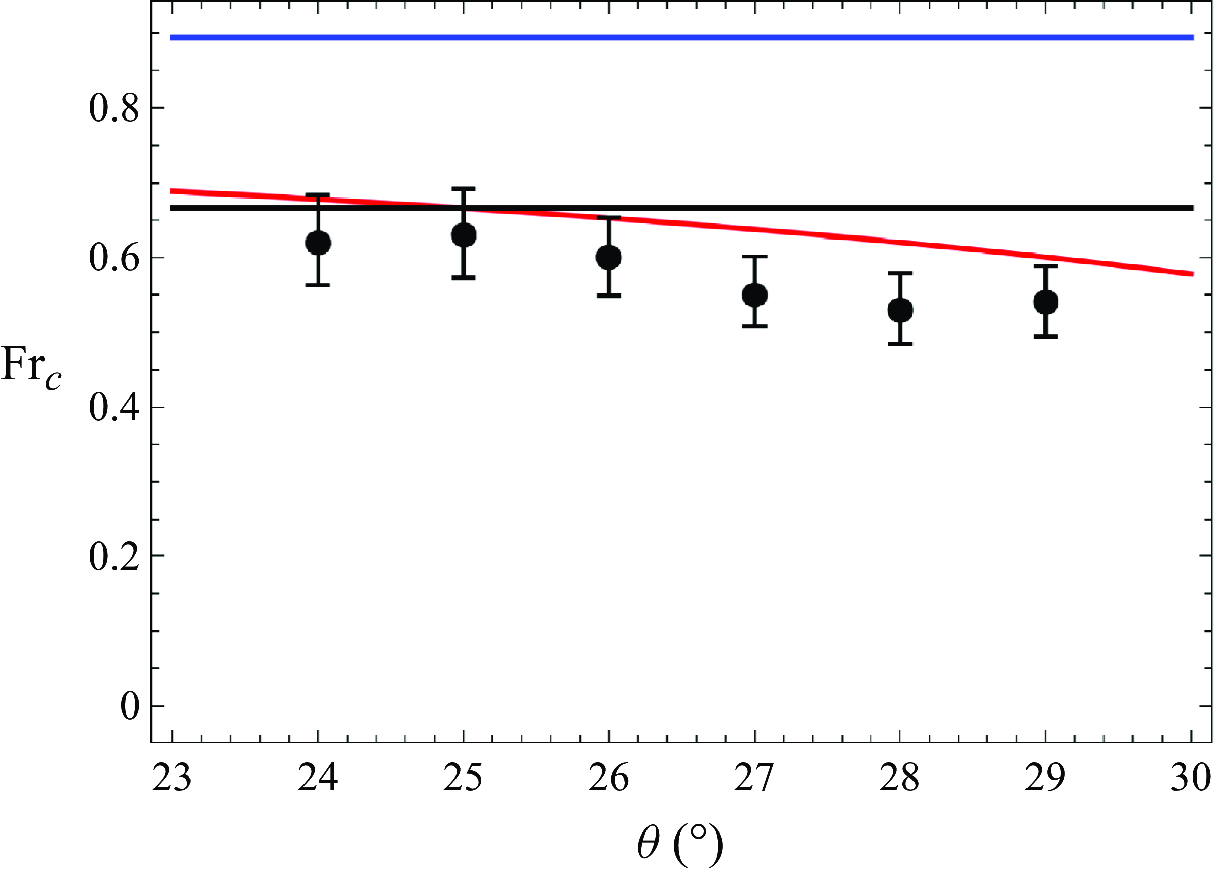
The variation of the consistent critical Froude number (present model and Forterre (Reference Forterre2006)) as a function of the inclination is presented in figure 2 (red curve) in the case of glass beads, using the values
 $\mu _1 = \tan 20.9^\circ$
and
 $\mu _2= \tan 32.76^\circ$
(Jop et al. Reference Jop, Forterre and Pouliquen2005), together with the experimental measurements of Forterre & Pouliquen (Reference Forterre and Pouliquen2003) (black dots). The stability criterion obtained with the two-equation model with or without diffusion (e.g. Forterre & Pouliquen Reference Forterre and Pouliquen2003; Gray & Edwards Reference Gray and Edwards2014) is also shown, with a shape factor of 1 (velocity constant over the depth, black line), or with a shape factor of
 $5/4$
(Bagnold velocity profile, blue line). These criteria differ from the criterion obtained with the
 $\mu (I)$
rheology because these Saint-Venant models, both with a shape factor of 1 or
 $5/4$
, are inconsistent approximations of the governing equations. The criterion obtained with a constant velocity profile (
 ${\mathcal F}_c =2/3$
) is paradoxically closer to the consistent criterion than with a shape factor of
 $5/4$
(
 ${\mathcal F}_c=2/\sqrt {5} \simeq 0.89$
) because some first-order terms were neglected in the derivation of the model. The systematic asymptotic expansions used to derive the present model enables us to obtain both a consistent stability criterion and a Bagnold velocity profile for steady uniform flows with its correction for flows in a non-equilibrium state (see also the discussion in § 5.5).
Critical Froude number as a function of the angle
 $\theta$
for glass beads. Theoretical value obtained with the
 $\mu (I)$
rheology (Forterre Reference Forterre2006) and given by the present model (red curve). Saint-Venant model with a shape factor of 1 (black line) and of
 $5/4$
(blue line) (Forterre & Pouliquen Reference Forterre and Pouliquen2003). Black dots: experimental measurements of Forterre & Pouliquen (Reference Forterre and Pouliquen2003).

Using the dispersion relation, it is also possible to express
 $k=k(\omega ,F)$
, where
 $\omega = ck$
. It is then possible to study the neutral stability curve defined by
 $\mathrm {Im}(k)=0$
(if
 $\omega$
is real). Computations (see Appendix B) show that
 $\partial F_c/\partial \omega |_{\omega =0}=0$
and that
 $\partial ^2F_c/\partial \omega ^2|_{\omega =0} = f(\lambda )$
, where
 $\lambda$
is the parameter introduced in § 4.2 and
 $f(\lambda )$
is a complicated function of
 $\lambda$
that vanishes when
 $\lambda$
has the value
 \begin{equation} \lambda = \frac {847(4-3C)}{20(157C+84)}. \end{equation}
If we use this expression of
 $\lambda$
, the expression (5.26) of the critical Froude number
 ${\mathcal F}_c$
and the expression
 $k=2\omega /5$
of the wavenumber, the dispersion relation is automatically satisfied. This implies that, for this value of
 $\lambda$
, the neutral stability curve
 $F=F(\omega )$
is obtained at the fixed value
 ${\mathcal F}_c$
of the Froude number independently of the frequency
 $\omega$
and that the phase velocity is also independent of the frequency on the neutral stability curve and equal to
 $5/2$
.
The independence of the critical Froude number from the frequency is obtained with all first-order two-equation hyperbolic models in every rheology if only weight, friction and fluxes are included (i.e. with no capillarity, diffusion or any other effect giving higher derivatives). The phase velocity is also independent of the frequency on the neutral stability curve. The proof is given in Appendix C. The behaviour of two-equation models is thus straightforward: the variation of the critical Froude number with frequency is only possible if diffusion is added to the model or other effects modelled with derivatives of high order such as capillarity (see Ruyer-Quil & Manneville Reference Ruyer-Quil and Manneville2002 for the effect of capillarity in a first-order model in the case of Newtonian fluids).
The mathematical structure of three-equation models allows a greater variety of behaviours, even for a first-order model without high-order derivatives. Consistency therefore does not imply model uniqueness, and modelling choices must be made that will determine the behaviour of the model outside the validity domain of the derivation assumptions. The choice is to reproduce with the three-equation model of first order the independence of the critical Froude number with frequency obtained with first-order two-equation models. The chosen expression of
 $\lambda$
also implies that the phase velocity is independent of the frequency on the neutral stability curve.
Another interesting feature of the choice (5.27) for
 $\lambda$
is that the stability condition can be found by the same argument as for two-equation models. It was shown by Whitham (Reference Whitham1974) that the stability condition for these models amounts to a condition on the kinematic wave velocity and the characteristic velocities: the steady uniform flow is stable if the kinematic wave velocity
 $a_0$
(whose value is
 $5/2$
in dimensionless form) is between the two characteristic velocities, i.e.
 $\lambda _- \lt a_0 \lt \lambda _+$
. This condition was applied to the case of granular flow models by Forterre & Pouliquen (Reference Forterre and Pouliquen2003) and Börzsönyi et al. (Reference Börzsönyi, Halsey and Ecke2005) in particular. For the three-equation model, the stability condition cannot be found with this simple argument except if
 $\lambda$
has the expression (5.27). In this particular case,
 $\lambda _- \lt a_0 \lt \lambda _+$
, which in practice reduces to
 $a_0 \lt \lambda _+$
, giving the condition (5.26).
Moreover, the choice (5.27) is supported by the satisfactory agreement of the spatial growth rate and phase velocity with the theoretical and experimental results and of the high-frequency extrapolation of the critical Froude number (see § 5.4 and figures 3, 4 and 5 below). For these reasons, the particular value (5.27) of
 $\lambda$
is the final choice for the model.
5.4. Adding diffusive effects
First-order models such as the present model (5.9) lead to some discrepancies due to the absence of diffusive terms (Forterre Reference Forterre2006; Andreotti et al. Reference Andreotti, Forterre and Pouliquen2013; Gray & Edwards Reference Gray and Edwards2014). The spatial growth rate in particular is not accurate far from the long-wave limit and the stabilisation of high frequencies is not predicted. Therefore, it is important to add diffusive terms to the model. These effects are of second order with respect to
 $\varepsilon$
but, since the second-order full consistency is very complicated and, moreover, does not yield well-posed models, only the linear terms due to the stress gradient in the streamwise direction are considered. The integration of (2.31) can be written as
 \begin{equation} \frac {\partial \tilde {h}\tilde {U}}{\partial \tilde {t}}+\frac {\partial }{\partial \tilde {x}}\left (\tilde {h}\tilde {U}^2+\tilde {h}^3\tilde{\psi}\right ) =\frac {1}{\varepsilon \phi F^2}\left (\!\phi \sin \theta \tilde {h}-\varepsilon \frac {\partial }{\partial \tilde {x}}\int _0^{\tilde {h}}\!\tilde {p}\mathrm {d}\tilde {z}-\tilde {\tau }_{xz}(0)+\varepsilon ^2 \!\int _0^{\tilde {h}}\frac {\partial \tilde {\tau }_{xx}}{\partial \tilde {x}}\mathrm {d}\tilde {z}\!\right ). \end{equation}
In this equation, only the second-order terms given by the integral of
 $\partial \tilde {\tau }_{xx}/\partial \tilde {x}$
are kept.
Equation (3.17) yields
 \begin{align} &\frac {\partial \tilde {\tau }_{xx}^{(0)}}{\partial \tilde {x}} = \phi \sin \theta \notag\\&\quad\times \left \{\left (\frac {\partial \tilde {h}}{\partial \tilde {x}}\right )^2\left [\left (1-\frac {\tilde {z}}{\tilde {h}}\right )^{1/2}+\left (1-\frac {\tilde {z}}{\tilde {h}}\right )^{-1/2}-2\right ] +2\frac {\partial ^2\tilde {h}}{\partial \tilde {x}^2}\left [\tilde {h}^{1/2}(\tilde {h}-\tilde {z})^{1/2}-\tilde {h}+\tilde {z}\right ]\right \}, \end{align}
which leads to
 \begin{equation} \int _0^{\tilde {h}}\frac {\partial \tilde {\tau }_{xx}^{(0)}}{\partial \tilde {x}} \, \mathrm {d}\tilde {z}= \frac {1}{3}\phi \sin \theta \frac {\partial }{\partial \tilde {x}}\left (\tilde {h}^2\frac {\partial \tilde {h}}{\partial \tilde {x}}\right ). \end{equation}
Using the expression (4.3) of
 $\tilde {U}^{(0)}$
, this term can be written as a diffusive term
 \begin{align} \int _0^{\tilde {h}}\frac {\partial \tilde {\tau }_{xx}^{(0)}}{\partial \tilde {x}}\, \mathrm {d}\tilde {z}= \phi F^2\frac {\partial }{\partial \tilde {x}}\left (\tilde {\nu }_{\textit{eff}}\tilde {h}\frac {\partial \tilde {U}^{(0)}}{\partial \tilde {x}}\right ), \end{align}
with an effective viscosity
 \begin{equation} \tilde {\nu }_{\textit{eff}} = \frac {5\sin \theta }{9\tilde {A}F^2}\tilde {h}^{1/2}. \end{equation}
Defining
 $\tilde \alpha _\nu$
by
 $\tilde \nu _{\textit{eff}}=\tilde \alpha _\nu \tilde h^{1/2}$
, we can write the depth-averaged momentum balance equation
 \begin{align} \frac {\partial \tilde {h}\tilde {U}}{\partial \tilde {t}}+\frac {\partial }{\partial \tilde {x}}\left (\tilde {h}\tilde {U}^2+\beta \tilde {h}^3\tilde{\psi}+K\frac {\cos \theta \tilde {h}^2}{2 F^2}\right ) &= \frac {\cos \theta }{\varepsilon F^2}\left [\tilde {h}(\tan \theta -\mu _b) + \frac {10\lambda }{\tilde {A}^2B}\left (\tilde{\psi}-\frac {\tilde {U}^2}{4\tilde {h}^2}\right )\right ] \nonumber \\&\quad +\varepsilon \frac {\partial }{\partial \tilde {x}}\left (\tilde {\alpha }_\nu \tilde {h}^{3/2}\frac {\partial \tilde {U}}{\partial \tilde {x}}\right ). \end{align}
The dimensionless effective viscosity obtained in Gray & Edwards (Reference Gray and Edwards2014) is similar, apart from a coefficient
 $1/F^2$
that comes from a different scaling. The expression of the effective viscosity in Forterre (Reference Forterre2006) is different but it is consistent at order 0 with (5.32).
We now need to take the diffusion into account in the energy equation. Technical details are given in Appendix D. Since we consider only linear terms, there is some freedom of choice for nonlinear terms that inevitably appear either in the enstrophy equation or in the energy equation or both. As for the first-order hyperbolic model, we impose conservation of enstrophy and dissipation of energy. Therefore, the enstrophy equation is written without nonlinear terms, which implies dissipative nonlinear terms in the energy equation. The enstrophy balance equation is thus written as
 \begin{align} \frac {\partial \tilde {h}\tilde{\psi}}{\partial \tilde {t}}+\frac {\partial \tilde {h}\tilde {U}\tilde{\psi}}{\partial \tilde {x}} &= \frac {2\tilde {U}\cos \theta }{\varepsilon \tilde {h}^2F^2}\left [\frac {\tilde {\alpha }_1}{\tilde {h}^{1/2}}\left (\tilde {U}-\frac {2}{5}\tilde {A}\tilde {h}^{3/2}\right )+ \tilde {\alpha }_2\left (\tilde{\psi}-\frac {\tilde {U}^2}{4\tilde {h}^2}\right )\right ]\notag\\&\quad + \varepsilon \frac {\partial }{\partial \tilde {x}}\left (\frac {16\tilde {\alpha }_\nu }{7\beta }\tilde {h}^{3/2}\frac {\partial \tilde{\psi}}{\partial \tilde {x}}\right ). \end{align}
The new depth-averaged energy balance equation is now found from the three equations of the system and can be written as
 \begin{align} \frac {\partial }{\partial \tilde {t}}\left (\tilde {h}\frac {\tilde {U}^2}{2}+\frac {\beta \tilde {h^3}\tilde{\psi}}{2}+K\frac {\tilde {h}^2\cos \theta }{2F^2}\right )+\frac {\partial }{\partial \tilde {x}}\left (\frac {\tilde {h}\tilde {U}^3}{2}+\frac {3\beta \tilde {h}^3\tilde {U}\tilde{\psi}}{2}+K\frac {\tilde {h}^2\tilde {U}\cos \theta }{F^2}\right ) \nonumber \\ = \frac {\tilde {U}\cos \theta }{\varepsilon F^2}\left [\tilde {h}(\tan \theta -\mu _b) + \frac {\beta \tilde {\alpha }_1}{\tilde {h}^{1/2}}\left (\tilde {U}-\frac {2}{5}\tilde {A}\tilde {h}^{3/2}\right )+\left (\beta \tilde {\alpha }_2+\frac {10\lambda }{\tilde {A}^2 B}\right )\left (\tilde{\psi}-\frac {\tilde {U}^2}{4\tilde {h}^2}\right )\right ]\nonumber \\ +\varepsilon \frac {\partial }{\partial \tilde {x}}\left (\tilde {\alpha }_\nu \tilde {h}^{3/2}\tilde {U}\frac {\partial \tilde {U}}{\partial \tilde {x}}\right )+\varepsilon \frac {\partial }{\partial \tilde {x}}\left (\frac {8\tilde {\alpha }_\nu }{7\beta }\tilde {h}^{7/2}\frac {\partial \tilde{\psi}}{\partial \tilde {x}}\right )-\varepsilon \tilde {\alpha }_\nu \tilde {h}^{3/2}\left (\frac {\partial \tilde {U}}{\partial \tilde {x}}\right )^2 -\varepsilon \frac {16\tilde \alpha _\nu }{7\beta }\tilde {h}^{5/2}\frac {\partial \tilde {h}}{\partial \tilde {x}}\frac {\partial \tilde{\psi}}{\partial \tilde {x}}. \end{align}
Reverting to the dimensional quantities, the system can be written as
 \begin{equation} \frac {\partial h}{\partial t}+\frac {\partial hU}{\partial x}=0, \end{equation}
 \begin{align} \frac {\partial hU}{\partial t}+\frac {\partial }{\partial x}\left (hU^2+\Pi \right ) &= g\cos \theta \left [h\left (\tan \theta -\mu _b\right )+\frac {10\lambda }{A^2B}\left (\psi -\frac {U^2}{4h^2}\right )\right ] \notag\\&\quad +\frac {\partial }{\partial x}\left (\alpha _\nu h^{3/2}\frac {\partial U}{\partial x}\right ), \end{align}
 \begin{align} \frac {\partial h\psi }{\partial t}+\frac {\partial hU\psi }{\partial x} &= \frac {2gU\cos \theta }{ h^2}\left [\frac {\alpha _1}{h^{1/2}}\left (U-\frac {2}{5}Ah^{3/2}\right )+\alpha _2\left (\psi -\frac {U^2}{4h^2}\right )\right ]\notag\\&\quad + \frac {\partial }{\partial x}\left (\frac {16 \alpha _\nu }{7\beta }h^{3/2}\frac {\partial \psi }{\partial x}\right ) , \end{align}
with the expressions of
 $A$
and
 $B$
given in (5.10), of
 $\alpha _1$
and
 $\alpha _2$
in (5.11), of
 $\lambda$
and
 $K$
in (5.12), of the basal friction
 $\mu _b$
in (5.13), with
 \begin{equation} \alpha _\nu =\frac {5g\sin \theta }{9A} \end{equation}
and
 \begin{equation} \Pi =\beta h^3 \psi + K\frac {gh^2}{2}\cos \theta . \end{equation}
The system admits the energy balance equation
 \begin{align} \frac {\partial he}{\partial t}&+\frac {\partial }{\partial x}\left (hUe+\Pi U\right ) = g U \cos \theta \nonumber \\ &\times \left [h(\tan \theta -\mu _b) + \frac {\beta \alpha _1}{h^{1/2}}\left (U-\frac {2}{5}Ah^{3/2}\right )+\left (\beta \alpha _2+\frac {10\lambda }{A^2B}\right )\left (\psi -\frac {U^2}{4 h^2}\right )\right ] \nonumber \\ &+\frac {\partial }{\partial x}\left ( \alpha _\nu h^{3/2} U\frac {\partial U}{\partial x}\right ) +\frac {\partial }{\partial x}\left (\frac {8 \alpha _\nu }{7\beta } h^{7/2}\frac {\partial \psi }{\partial x}\right ) - \alpha _\nu h^{3/2}\left (\frac {\partial U}{\partial x}\right )^2 - \frac {16 \alpha _\nu }{7\beta } h^{5/2}\frac {\partial h}{\partial x}\frac {\partial \psi }{\partial x} ,\end{align}
with the specific energy
 $e$
given by (5.16).
The dispersion relation is modified by the diffusive terms. Taking again sinusoidal perturbations of the form
 $\tilde {h} =1+h'$
,
 $\tilde {U}=\tilde {U}^{(0)}+U'$
and
 $\tilde{\psi}=\tilde{\psi}^{(0)}+\psi '$
, the linearised system now reads
 \begin{equation} M_V(\varepsilon )\begin{pmatrix} h' \\ U' \\ \psi ' \end{pmatrix} =0,\qquad \text{with }\ M_V(\varepsilon )=\frac {\cos \theta }{F^2}R+i\varepsilon k L + \varepsilon ^2 k^2 \tilde {\alpha }_\nu V, \end{equation}
where
 $R$
,
 $L$
are defined in (5.21), (5.20) and
 $V$
is the matrix of the linearised viscous terms, given by
 \begin{equation} V= \begin{pmatrix} 0 & 0 & 0\\ 0 & 1 & 0 \\ 0 & 0 & \frac {16}{7\beta } \end{pmatrix}. \end{equation}
The new dispersion relation is
 $\det (M_V)= 0$
. We now suppose that
 $\omega = ck\in \mathbb {R}$
and that
 $k$
is complex. The spatial growth rate is then given by
 $\sigma = -\mathrm {Im}(k)$
. The system is stable if and only if
 $\sigma \lt 0$
.
Spatial dimensionless growth rate for
 $\theta = 29^\circ$
and
 ${\mathcal F} =1.02$
as a function of the dimensionless frequency. Black dots: experimental measurements of Forterre & Pouliquen (Reference Forterre and Pouliquen2003). Red solid curve: present model with diffusion. Black curve : theoretical result for the
 $\mu (I)$
rheology (Forterre Reference Forterre2006). Two-equation model without diffusion (e.g. Forterre & Pouliquen Reference Forterre and Pouliquen2003) with a shape factor
 $\alpha =1$
(green dashed curve) and
 $\alpha =5/4$
(blue dashed curve) and with diffusion (Gray & Edwards Reference Gray and Edwards2014) with a shape factor
 $\alpha =1$
(green solid curve) and
 $\alpha =5/4$
(blue solid curve).

The variations of the dimensionless spatial growth rate
 $\sigma$
with the dimensionless angular frequency are presented in figure 3 for the present model with diffusion (red curve) and
 $\lambda$
given by (5.27), in the case of glass beads (
 $\mu _1 = \tan 20.9^\circ$
,
 $\mu _2= \tan 32.76^\circ$
, Jop et al. (Reference Jop, Forterre and Pouliquen2005)) and for
 $\theta = 29^\circ$
and
 ${\mathcal F} =1.02$
. The results are compared with the theoretical results obtained for the
 $\mu (I)$
rheology by Forterre (Reference Forterre2006) (black curve) and with the experimental measurements of Forterre (Reference Forterre2006) (black dots). The two-equation models without diffusion derived with a constant velocity profile (green dashed curve) and with a Bagnold profile (blue dashed curve) are also presented together with the model with diffusion (Gray & Edwards Reference Gray and Edwards2014) (green curve if
 $\alpha =1$
, blue curve if
 $\alpha =5/4$
).
The curve obtained with the present model with diffusion is very close to the curve obtained by Gray & Edwards (Reference Gray and Edwards2014). Both models predict quite correctly the stabilisation of high frequencies, with a cutoff frequency, and are in reasonable agreement with the experimental measurements and with the theoretical result for the
 $\mu (I)$
rheology. By contrast, the Saint-Venant models cannot predict the cutoff frequency due to the absence of diffusive terms. These Saint-Venant models are also inconsistent approximations of the governing equations but the inaccuracy is much more important for the model with a shape factor of
 $5/4$
(Bagnold profile). The present model is also based on a Bagnold velocity profile at leading order but it gives accurate results because of the consistent asymptotic expansions used in its derivation.
The dimensionless phase velocity
 $c$
is presented in figure 4 (same conditions as for figure 3). The present model with diffusion and
 $\lambda$
given by (5.27) (red curve) is in good agreement with the theoretical result for the
 $\mu (I)$
rheology (black curve) and with the experimental measures (Forterre Reference Forterre2006). The model of Gray & Edwards (Reference Gray and Edwards2014) with diffusion (green solid curve) gives practically the same result as the model without diffusion (Forterre & Pouliquen Reference Forterre and Pouliquen2003, green dashed curve), and agrees with the theoretical and experimental results if a flat velocity profile is considered, i.e.
 $\alpha =1$
, while the models with a Bagnold profile (
 $\alpha =5/4$
), with (blue solid curve) or without (blue dashed curve) diffusion, give values clearly too large. In this case again, the consistent derivation used for the present model improves the accuracy of the predictions when a Bagnold velocity profile is considered for steady uniform flows. The value of the dimensionless phase velocity for
 $\omega =0$
is the celerity
 $\tilde {A}\tilde {h}^{3/2}=5/2$
of the kinematic waves while the phase velocity for
 $\omega \to \infty$
is the characteristic velocity
 $\lambda _+$
, whose value is
 $1 + \sqrt {K/F^2 + 3\beta /4}=2.07$
for the present model if
 $\lambda$
is given by (5.27), and
 $1+1/F = 1.98$
for the two-equation models with
 $\alpha = 1$
. The difference between these two high-frequency limit values is due to the Bagnold profile taken into account by the enstrophy, whose equilibrium value is
 $1/4$
if the equilibrium velocity is
 $1$
, and to the consistency factors
 $K$
and
 $\beta$
, which depend on the choice of
 $\lambda$
. The critical expression (5.27) of
 $\lambda$
gives results in good agreement with the experimental and theoretical results both for the spatial growth rate and the phase velocity.
Dimensionless phase velocity for
 $\theta = 29^\circ$
and
 ${\mathcal F} =1.02$
as a function of the dimensionless frequency. Black dots: experimental measurements of Forterre & Pouliquen (Reference Forterre and Pouliquen2003). Red solid curve: present model with diffusion. Black curve : theoretical result for the
 $\mu (I)$
rheology (Forterre Reference Forterre2006). Two-equation model without diffusion (e.g. Forterre & Pouliquen Reference Forterre and Pouliquen2003) with a shape factor
 $\alpha =1$
(green dashed curve) and
 $\alpha =5/4$
(blue dashed curve) and with diffusion (Gray & Edwards Reference Gray and Edwards2014) with a shape factor
 $\alpha =1$
(green solid curve) and
 $\alpha =5/4$
(blue solid curve).

Dimensionless cutoff frequency
 $\omega _c$
of the instability as a function of the Froude number above criticality
 ${\mathcal F}-{\mathcal F}_c$
for
 $\theta =29^\circ$
. Black dots: experimental measurements of Forterre & Pouliquen (Reference Forterre and Pouliquen2003). Present model with diffusion for
 $\lambda$
given by (5.27) (red solid curve),
 $\lambda = 0$
(blue curve) and
 $\lambda = 11/4$
(green curve). Red dashed curve: present model without diffusion for
 $\lambda$
given by (5.27). Black curve: theoretical result for the
 $\mu (I)$
rheology (Forterre Reference Forterre2006).

The variations of the dimensionless cutoff angular frequency
 $\omega _c$
as a function of the Froude number above criticality
 ${\mathcal F}-{\mathcal F}_c$
is presented in figure 5 for glass beads and
 $\theta =29^\circ$
. As pointed out above, there is no uniqueness of a first-order consistent model. The value of the parameter
 $\lambda$
is a modelling choice. The choice that has been made, detailed above at the end of § 5.3, is to have a critical Froude number independent of frequency for the model without diffusion. This choice leads to the critical value (5.27).
Other special values of
 $\lambda$
include
 $\lambda =0$
and
 $\lambda =11/4$
. In the case
 $\lambda =0$
, there is no relaxation term for the enstrophy in the momentum balance equation and the first-order correction to the granular friction law is entirely written as terms in the momentum flux. In the case
 $\lambda = 11/4$
, we have
 $\beta =1$
, which means that there is no correction on the shear term
 $h^3\psi$
in the momentum flux although, since
 $K\lt 1$
, there is still a correction on the pressure term of the momentum flux (the value of
 $\lambda$
needed to have
 $K=1$
is
 $21/4$
, so even higher). In the final choice (5.27), part of the first-order correction is written in the momentum flux, with a correction on both the enstrophy and pressure terms, and another part as a relaxation term.
The effect of the parameter
 $\lambda$
is shown with the model with diffusion in these three cases:
 $\lambda$
is equal to the critical value (5.27) (red solid curve),
 $\lambda =0$
(blue curve) and
 $\lambda =11/4$
(green curve). Since all these values of
 $\lambda$
give a consistent model, they lead to the same result in the validity domain of the shallow-water approximation, thus for small frequencies, but this domain is quite small (
 $\tilde {\omega }\lt 0.1$
approximately). For larger frequencies, the cutoff frequency is sensitive to the choice of
 $\lambda$
. For the critical value of
 $\lambda$
(5.27), the agreement of the model with diffusion with the theoretical result for the
 $\mu (I)$
rheology (black curve) and with the experimental results (black dots), both obtained by Forterre (Reference Forterre2006), is quite good. For smaller values of
 $\lambda$
, and in particular for
 $\lambda =0$
, there are unstable frequencies that are smaller than the cutoff at the long-wave limit, which does not seem to be observed experimentally. For larger values of
 $\lambda$
, the cutoff frequency is too small. The diffusion is again important to stabilise the high frequencies. Only the case
 $\theta =29^\circ$
is presented, but other values of
 $\theta$
studied by Forterre (Reference Forterre2006) and Gray & Edwards (Reference Gray and Edwards2014) show the same trends.
5.5. Comparisons with the model of Gray & Edwards (Reference Gray and Edwards2014)
The model of Gray & Edwards (Reference Gray and Edwards2014) with diffusion was used for many applications (see § 1). It is therefore important to compare the model derived in this paper with this model, highlighting the differences and similarities between these two models.
The model of Gray & Edwards (Reference Gray and Edwards2014) was proposed with a shape factor
 $\alpha$
in the momentum flux, defined by
 $\langle u^2 \rangle = \alpha \langle u \rangle ^2$
. Two values of
 $\alpha$
were considered: The value
 $\alpha = 5/4$
corresponds to a Bagnold velocity profile while the value
 $\alpha = 1$
corresponds to a constant velocity in the depth. Although this difference in the value of
 $\alpha$
seems minor, it induces a significant change in mathematical structure and behaviour, to the extent that these two values correspond to two different models. In most applications,
 $\alpha = 1$
was the only value used.
Whatever the value of
 $\alpha$
, the derivation of the model of Gray & Edwards (Reference Gray and Edwards2014) is inconsistent, in the sense that first-order corrections have been neglected. In particular, gravity balances friction at leading order, and their difference is of
 $O(\varepsilon )$
. To achieve the first-order accuracy required for consistent modelling of variable flows, this difference cannot be neglected and the corresponding first-order correction must be included in the model. As a result, the instability threshold for steady uniform flows calculated with the model of Gray & Edwards (Reference Gray and Edwards2014), as with the model of Pouliquen & Forterre (Reference Pouliquen and Forterre2002), differs from the threshold predicted by the
 $\mu (I)$
rheology calculated at the long-wave limit by Forterre (Reference Forterre2006). By contrast, the present model is first-order consistent and predicts exactly the same instability threshold as the
 $\mu (I)$
rheology in the long-wave limit.
The discrepancy of the instability threshold predicted by the model of Gray & Edwards (Reference Gray and Edwards2014), or any other similar two-equation model, can be particularly large if
 $\alpha =5/4$
. It is more reasonable if
 $\alpha =1$
. In the case of glass beads down a slope of
 $29^{\circ }$
, the measurements of Forterre & Pouliquen (Reference Forterre and Pouliquen2003) gave a value of the critical Froude number
 ${\mathcal F}_c =0.54 \pm 0.02$
at the zero-frequency limit, whereas the
 $\mu (I)$
rheology and the present model predict
 ${\mathcal F}_c =0.60$
, giving a relative deviation of
 $11\%$
. The models of Gray & Edwards (Reference Gray and Edwards2014) and Pouliquen & Forterre (Reference Pouliquen and Forterre2002) give
 ${\mathcal F}_c = 2/3$
with
 $\alpha =1$
(relative deviation:
 $23\%$
) and
 ${\mathcal F}_c \simeq 0.89$
if
 $\alpha =5/4$
(relative deviation:
 $65\%$
).
The consistency of the derivation of the present model enables us to reconstruct the velocity profile in the depth. This profile is a Bagnold profile for a steady uniform flow, but the reconstruction allows us to calculate the deviations from this profile due to first-order corrections when the flow is variable. This reconstruction is not possible with the model of Gray & Edwards (Reference Gray and Edwards2014), particularly if
 $\alpha =1$
, which corresponds to a constant velocity profile for steady uniform flows. If
 $\alpha =5/4$
, the equilibrium profile is a Bagnold profile, but the corrections for variable flows cannot be calculated. One of the advantages of introducing the enstrophy variable is that the velocity profile is not fixed as with a shape factor. With a shape factor of
 $5/4$
, the velocity profile is always a Bagnold profile, even for a variable flow. With the present model, thanks to the enstrophy variable, the profile is a Bagnold profile for a steady uniform flow but the model takes into account and calculates the corrections to this profile in the case of a variable flow.
With the model of Gray & Edwards (Reference Gray and Edwards2014) with
 $\alpha =5/4$
, no energy balance equation can be obtained (see the general proof in Appendix A of Richard & Gavrilyuk Reference Richard and Gavrilyuk2012). By contrast, the model with
 $\alpha =1$
and the present model are well-posed because both admit an energy balance equation. This is an important feature for physical reasons but also from a numerical point of view, since the energy conservation is essential to prove the stability of numerical schemes. The characteristics of the model with
 $\alpha =5/4$
are also completely different from those of the model with
 $\alpha =1$
. They are also much more complicated. For these reasons, the mathematical structure of the model of Gray & Edwards (Reference Gray and Edwards2014) changes radically when the value of the shape factor increases from
 $1$
to
 $5/4$
.
The predictions and the mathematical structure of the model of Gray & Edwards (Reference Gray and Edwards2014) are paradoxically better if a constant velocity profile is assumed (i.e. if
 $\alpha =1$
) than if a Bagnold profile is taken into account (
 $\alpha =5/4$
). This paradox, noted by Forterre & Pouliquen (Reference Forterre and Pouliquen2003), is resolved by the present model, which obtains both accurate results and a Bagnold profile at equilibrium, thanks to the consistency of its derivation. Since it is hyperbolic (disregarding the diffusive terms), in conservative form, and with an exact energy conservation equation, the present model has also a good mathematical structure.
The diffusion term is the same in the present model and in the model of Gray & Edwards (Reference Gray and Edwards2014). Since this term is of second order, it can be consistently calculated assuming a Bagnold velocity profile (zero-order solution). In this respect, the present work confirms the expression already found by Gray & Edwards (Reference Gray and Edwards2014) for the diffusive term. It follows that properties depending on the diffusive term, such as the variations of the spatial growth rate or of the phase velocity with frequency, are equivalent with this model and the model of Gray & Edwards (Reference Gray and Edwards2014) with
 $\alpha =1$
. With the value
 $\alpha =5/4$
, the two-equation models, even with diffusion, lead to a large discrepancy in the spatial growth rate and the phase velocity (see figures 3 and 4).
Dimensionless cutoff frequency
 $\omega _c$
of the instability as a function of the Froude number
 ${\mathcal F}$
for
 $\theta =29^\circ$
. Black dots: experimental measurements of Forterre & Pouliquen (Reference Forterre and Pouliquen2003). Present model with diffusion for
 $\lambda$
given by (5.27) (red solid curve). Green curve: model of Gray & Edwards (Reference Gray and Edwards2014) with
 $\alpha =1$
. Black curve: theoretical result for the
 $\mu (I)$
rheology (Forterre Reference Forterre2006).

The model of Gray & Edwards (Reference Gray and Edwards2014) with
 $\alpha =1$
and the present model are compared with regard to the variation of the cutoff frequency with the Froude number. In figure 5, all variants of the model were consistent to the
 $\mu (I)$
rheology. Variations in cutoff frequency could be studied as a function of the difference between the Froude number and its critical value. In this comparison, the critical Froude number predicted by both models are different. The variation of the cutoff frequency as a function of the Froude number
 ${\mathcal F}$
is shown in figure 6 with the curve predicted by the
 $\mu (I)$
rheology calculated by Forterre (Reference Forterre2006) (black), the experimental measurements of Forterre & Pouliquen (Reference Forterre and Pouliquen2003) (black dots), the present model (red curve) and the model of Gray & Edwards (Reference Gray and Edwards2014) (green curve). The main difference between the two models is the value of the critical Froude number, i.e. the beginning of the curves at the limit of a zero frequency. Since the diffusive term is the same in both models, and the variations in cutoff frequency with Froude number are due to the diffusive term, both models predict fairly similar variations apart from the starting point of the curves.
The mathematical structure of the model of Gray & Edwards (Reference Gray and Edwards2014) with
 $\alpha =1$
is the structure of the Saint-Venant equations (or nonlinear shallow-water equations) with an additional diffusive term. The structure of the present model is the structure of the compressible Euler equation with source terms and additional diffusive terms. Both structures are well known and can be solved numerically with classical and reliable numerical schemes. We do not recommend solving numerically the model with
 $\alpha =5/4$
, as no guarantee can be given regarding the numerical scheme.
5.6. Numerical resolution
In this subsection we solve numerically the model in order to study the roll waves instability. The numerical solution is calculated with a Godunov-type scheme (HLLC Riemann solver). We solve system (5.9) in the conservative variables
 $(h,hU,h\psi )$
. In these variables the total energy plays the role of a mathematical entropy for the system. The relaxation source terms are implemented explicitly. The second-order diffusion terms are approximated by centred finite differences. We use the following parameters:
 $\mu _1 = \tan (20.9^\circ )$
,
 $\mu _2 = \tan (32.76^\circ )$
,
 $I_m = 0.279$
(see Jop et al. Reference Jop, Forterre and Pouliquen2006),
 $d=5\times 10^{-4}$
m,
 $\theta = 25^\circ$
,
 $\phi = 0.6-0.2\, I^{(0)}$
(see (3.10)),
 $g=9.81$
ms-1
and
 $h_0=10^{-2}$
m. It follows that
 ${\mathcal F}\approx 0.806\gt {\mathcal F}_c\approx 0.666$
.
The domain has a length of
 $100\,\mathrm {m}$
. The initial conditions are a steady uniform flow of depth
 $h_0$
, average velocity
 $U_0=2Ah_0^{3/2}/5$
and enstrophy
 $\psi _0=U_0^2/(4h_0^2)$
. The boundary condition at the domain entrance is a small sinusoidal perturbation of the depth
 $h(0,t)=h_0[1+\alpha _0 \sin (2\pi ft)]$
. The relative amplitude and frequency of the perturbation are
 $\alpha _0=0.01$
and
 $f=0.316\, \mathrm {Hz}$
, respectively. The inlet values of the velocity and enstrophy are
 $U(0,t)=h_0 U_0 / h(0,t)$
and
 $\psi (0,t)=(h_0U_0)^2/(4h(0,t)^4)$
, respectively. The results are presented with a cell size of
 $0.625\, \mathrm {mm}$
in order to reach numerical convergence with the diffusive model and a numerical scheme of order 1.
In the beginning, the amplitude of the perturbation increases exponentially. After some time, the amplitude converges to a maximal value. A steady state is then reached and the solution becomes periodic. This is illustrated by figure 7, which shows the height of the flow for the system (5.9) (purely hyperbolic) and for the system (5.36)–(5.38) (with diffusion terms). The depth profiles of the two systems are similar. It can be seen that, in the presence of diffusion, the amplitude of the waves is slightly smaller and the propagation is slightly slowed. As expected, the shock is steeper in the purely hyperbolic model. However, the effects of the diffusive terms seem to have little overall impact on the global shape of the solution. This is coherent with the fact that the diffusive terms are of order
 $\varepsilon ^2$
in our asymptotic expansions. Figure 8 shows the values taken by the basal friction
 $\mu _b$
and the enstrophy
 $\psi$
over a period, once the steady state is reached. The basal friction decreases when the depth increases, while the enstrophy increases. If the inlet perturbation is smaller, the length required to reach the steady state is longer but the steady-state waves are the same.


Finally, the horizontal velocity profile is reconstructed in figure 9, with the help of (5.8). The reconstructions are presented for three different values of
 $x$
. The black curve is obtained by reconstruction of the velocity at the wave trough. It is very close to a Bagnold profile (solution at equilibrium). The red curve is obtained by reconstruction at the wave crest. The blue curve is obtained at an intermediate state. As the height increases, the profile becomes more and more curved. The first-order correction with respect to the leading-order velocity profile, which represents the deviation of the velocity profile from the Bagnold profile, can be visualised by the difference between the red/blue curve and the black curve.
Reconstruction of the velocity profile for the numerical simulation of § 5.6. Black line: profile at the wave trough (just after the shock); red line: profile at the wave crest; blue line: profile where the height of the perturbation reaches
 $80\%$
of the maximal height.

6. Limitations of the model
It is essential to regularise the model for certain values of the angle
 $\theta$
because some quantities of the system (5.36)–(5.38) may change sign or become infinite, resulting in a ill-posed model.
In order to understand why this can happen, let us recall some facts about the
 $\mu (I)$
rheology. As mentioned in the first section, this rheology corresponds to a friction law, for which the friction coefficient is given by
 \begin{equation} \mu (I) = \mu _1 + \frac {\mu _2-\mu _1}{1+I_m/I}. \end{equation}
The two parameters
 $\mu _1$
and
 $\mu _2$
are determined experimentally. They characterise the angles for which steady uniform flows can be observed. These steady uniform flows only exist when
 \begin{equation} \mu _1\lt \tan \theta \lt \mu _2. \end{equation}
Outside this range, there is no equilibrium and all the formulas that we obtained previously do not make any sense a priori. We insist on the fact that the model (5.36)–(5.38) is derived with an asymptotic method, under the hypotheses that
 $\theta$
is constant and inside this range, so that the flow remains close to the uniform stationary flow. However, for geophysical applications, the value of the slope may not lie within the interval
 $[\mu _1,\mu _2]$
.
Recall that the expression of the inertial number
 $I$
at leading order is
 \begin{equation} I^{(0)}=I_m\frac {\tan \theta -\mu _1}{\mu _2-\tan \theta }. \end{equation}
This expression is only valid when condition (6.2) is verified and makes no sense otherwise. The following special cases are of particular importance:
-
(i) In the limit
$\tan \theta \rightarrow \mu _1$
, we have
$I^{(0)}\rightarrow 0$
. It follows that
$U^{(0)}$
and
$\psi ^{(0)}$
both converge to 0 and the flow should stop. This is called the liquid/solid transition. On the right-hand side of the system (5.36)–(5.38), the relaxation coefficients as well as the diffusion coefficients diverge to
$+\infty$
, which indicates that
$U$
and
$\psi$
should go to zero instantaneously. Given that this is likely to cause problems for numerical resolution and that the instantaneous stopping of an avalanche is not physical, these coefficients need to be regularised. In addition, the frictional hysteresis is not taken into account by the model derivation assumptions. -
(ii) In the limit
$\tan \theta \rightarrow \mu _2$
,
$I^{(0)}\rightarrow +\infty$
. The relaxation and diffusion coefficients go to zero. This is the liquid/gas transition, after which the flow becomes uniformly accelerated and enters a kinetic regime in which the volume fraction decreases. For
$\tan \theta \gt \mu _2$
, the effective viscosity becomes negative, requiring regularisation. Beyond this limit, the flow is no longer correctly described either by the
$\mu (I)$
rheology or, consequently, by the model, which means that the equations have to be modified. -
(iii) Finally, another singularity of the model can appear when the coefficient
$\mu _2$
is large. Indeed, recall that the stability criterion in the long-wave limit is(6.4)where
\begin{equation} {\mathcal F}^2\lt {\mathcal F}_c^2=\frac {16}{25}(4-3C), \end{equation}
$C=C(\theta )$
is an increasing function of
$\theta$
that is equal to
$2\mu _2^2$
when
$\tan \theta =\mu _2$
. If
$\mu _2\lt \sqrt {2/3}$
, the condition
$C\lt 4/3$
is automatically satisfied for a slope in the range
$[\mu _1,\mu _2].$
If
$\mu _2\gt \sqrt {2/3}\approx 0.816$
, there are some values of
$\theta$
that verify (6.2) for which every steady flow is unstable, even when
${\mathcal F}=0$
, because
$C\gt 4/3$
(which gives
${\mathcal F}_c^2\lt 0$
!). This phenomenon is inherent to the
$\mu (I)$
rheology since the stability criterion is the same for the bulk equations, as shown by Forterre (Reference Forterre2006). In the system (5.36)–(5.38), it is materialised by the fact that the sign of the relaxation coefficient
$\alpha _2$
changes when the critical Froude number is equal to zero (see § 4.3 above), as well as the sign of the coefficient
$K$
in front of the hydrostatic pressure and of the potential energy term in the expression (5.16) of the energy. In particular, the enstrophy
$\psi$
grows exponentially in this case and the system is ill-posed. Furthermore, the hyperbolicity of the system is not guaranteed anymore when
$C\gt 4/3$
(see § 5.2). It is not clear whether this instability effect has a real physical meaning or if it is only a shortcoming of the rheology. In the literature, the value of
$\mu _2$
is often lower than the critical value
$\sqrt {2/3}$
(
$\mu _2=\tan 32.76^\circ \approx 0.643$
in Jop et al. (Reference Jop, Forterre and Pouliquen2006) for instance). However, the value of
$\mu _2$
was
$\mu _2=1$
for the experiments of Börzsönyi & Ecke (Reference Börzsönyi and Ecke2006). They observed steady flows only under a critical angle
$\tan \theta \approx 0.85$
, above which the flow became uniformly accelerated. With their parameters, this corresponds to a value of
$C(\theta )\approx 1.36$
, which is close to the theoretical value
$C=4/3\approx 1.33$
that we obtained for the instability of the model. Further investigations need to be performed to see whether this is a coincidence or a successful prediction of the
$\mu (I)$
rheology. In any case, this instability also requires regularisation.


We use the term ‘regularisation’ here in a very broad sense. By regularisation, we mean a shift in the model towards physical behaviours obeying laws and assumptions that can be very different, and not just mathematical procedures. The physical phenomena that appear outside the model’s domain of validity are complex and not always well known. How to capture them in the model is also a complex problem that does not necessarily have a unique solution. A regularised system should be usable for numerical simulations with any value of the slope. However, the development of such a regularised model requires an in-depth study of flow stopping, of accelerated flows and of granular avalanche fronts, which is beyond the scope of this paper and will be the subject of a future work.
In particular, the flow near the head of a granular front does not meet the assumptions of a shallow flow. Consequently, the characteristics of such a flow may differ greatly from a steady uniform flow, with the result that the asymptotic method may be irrelevant. Saingier et al. (Reference Saingier, Deboeuf and Lagrée2016) and Lagrée et al. (Reference Lagrée, Saingier, Deboeuf, Staron and Popinet2017) showed that, while a Bagnold velocity profile was in good agreement with experimental results, the shape coefficient tends towards
 $\alpha = 1$
near the head of the front. This is the same value as for a constant velocity in depth. This raises the question of the velocity profile in this part of the flow. The model used in this work is therefore not yet suitable for treating granular avalanche fronts and, for this case too, a regularisation will be necessary.
The ill-posed nature of the model for liquid/solid or liquid/gas transitions is a consequence of the limitations of the
 $\mu (I)$
rheology to these same transitions. The limitations of the rheology for quasi-static regimes have been highlighted by many authors (see, e.g., GDR MiDi 2004; Andreotti et al. Reference Andreotti, Forterre and Pouliquen2013). For these regimes, the simple assumption of a local rheology is not valid. Large spatial correlation lengths diverging at the quasi-static limit, as well as mechanical noise, could explain the appearance of non-local effects. Various non-local laws have been proposed for the rheology (see, e.g., Pouliquen & Forterre Reference Pouliquen and Forterre2009; Kamrin & Koval Reference Kamrin and Koval2012; Bouzid et al. Reference Bouzid, Izzet, Trulsson, Clément, Claudin and Andreotti2015; Kamrin & Henann Reference Kamrin and Henann2015; Kamrin Reference Kamrin2019; Gaume, Chambon & Naaim Reference Gaume, Chambon and Naaim2020). The dilute regime at the transition to the gaseous regime described by the kinetic theory of granular gases is not predicted by the
 $\mu (I)$
rheology either. It is therefore not surprising that a model consistent with the
 $\mu (I)$
rheology is characterised by the same limitations as the rheology itself.
On the other hand, the limitations of the model are not directly related to the ill-posed behaviour of the
 $\mu (I)$
rheology found by Barker et al. (Reference Barker, Schaeffer, Bohórquez and Gray2015) at the high-wavenumber limit. The model is derived at the long-wave limit and has a mathematical structure similar to the structure of the compressible Euler equations with source terms and diffusion terms. Even the possible singularity that can arise if
 $\mu _2\gt \sqrt {2/3}$
is found at the long-wave limit, as in Forterre (Reference Forterre2006). The model is always well-posed for
 $\mu _1\lt \tan \theta \lt \mu _2$
if
 $\mu _2\lt \sqrt {2/3}$
and for
 $\mu _1\lt \tan \theta \lt \sqrt {2/3}$
if
 $\mu _2\gt \sqrt {2/3}$
, which is a wider range of stability than the range found in Barker et al. (Reference Barker, Schaeffer, Bohórquez and Gray2015). It follows that the depth-averaging process at the long-wave limit eliminates the ill-posed behaviour at high wavenumbers found by Barker et al. (Reference Barker, Schaeffer, Bohórquez and Gray2015), who noted that ‘it is therefore possible to push the depth-averaged
 $\mu (I)$
rheology somewhat further than the full rheology’ and this has allowed us to calculate roll waves ‘using the depth-averaged theory, without getting into issues of ill-posedness’.
7. Conclusion
In this work we derive a new depth-averaged model for an incompressible granular flow described by the
 $\mu (I)$
rheology. The derivation is made using a consistent asymptotic method under the assumption of shallow flows. This method implies that, unlike the models derived to date for the
 $\mu (I)$
rheology such as Forterre & Pouliquen (Reference Forterre and Pouliquen2003) or Gray & Edwards (Reference Gray and Edwards2014), the model is consistent at the first order, with respect to the small shallow-flow parameter, with the
 $\mu (I)$
rheology. In particular, for the first time, the first-order correction to the classical granular friction law is included in the model. For steady uniform flows, the model is consistent with a Bagnold velocity profile, which is found at leading order. Otherwise, the model includes the first-order correction to this profile. This model resolves the paradox of previous models, for which the inclusion of a Bagnold profile led to a much greater disagreement with experimental and theoretical results than a constant velocity in the depth. Since the model is consistent, and in contrast to previous models, it gives the exact stability criterion of the
 $\mu (I)$
rheology in the long-wave limit as found by Forterre (Reference Forterre2006).
The resulting three-equation model is a hyperbolic system of conservation laws for the flow depth, the depth-averaged velocity and an additional quantity, called enstrophy, which takes into account shear effects. This system admits an exact energy balance equation. The model has the classical structure of the compressible Euler equations with relaxation source terms, which is well suited for numerical resolution. In contrast to the two-equation models with a shape factor of
 $5/4$
, this three-equation structure remains well-posed while taking into account a Bagnold velocity profile for steady uniform flows.
Thanks to the consistency of the asymptotic method used for the derivation, the variation in the depth of the velocity can be reconstructed explicitly with the three variables of the depth-averaged model. The deviations to the Bagnold profile can thus be calculated for flows that are not steady and uniform, such as granular roll waves.
This hyperbolic model is also extended to include diffusive effects. We confirm the expression of the effective viscosity obtained by Gray & Edwards (Reference Gray and Edwards2014), which is indeed the consistent form resulting from the application of the asymptotic method. The spatial growth rate and the phase velocity predicted by this extended model is in good agreement with both the theoretical predictions of the
 $\mu (I)$
rheology and with the experimental data of Forterre & Pouliquen (Reference Forterre and Pouliquen2003). In particular, the extended model predicts successfully the stabilisation of high frequencies and the variation of the cutoff frequency with the Froude number.
In this respect, it is important to note that it is possible to derive an infinite number of consistent models, all of which are equivalent within the validity domain of the long-wave approximation, but differ outside this domain. Outside the domain of validity of the shallow-flow assumption, the three-equation structure can produce a greater variety of behaviours than the two-equation structures. The best variant among the different possible consistent models was selected to obtain a critical Froude independent of the frequency for the model without diffusion, as in the case of non-diffusive two-equation models. In this variant, the instability threshold can be found by writing that the kinematic wave velocity lies between the maximum and minimum characteristic velocities, again as for two-equation models. This choice is also supported by the high-frequency extrapolation of the model with diffusion regarding the spatial growth rate, the phase velocity and the critical Froude number.
Numerical simulations of granular roll waves are presented, using classical finite-volume schemes with an approximate Riemann solver. All depth-averaged quantities can be calculated and the velocity profiles in the depth can be easily reconstructed.
The asymptotic method used to derive the model assumes that the flow remains close to the steady uniform flow and, therefore, that such a steady uniform flow exists. In the context of the
 $\mu (I)$
rheology, a steady uniform flow is only possible within a certain range of the angle of inclination of the bottom with respect to the horizontal. This range defines the model’s domain of validity. Outside this range, certain model quantities become infinite or change sign, and the model becomes mathematically ill-posed. This problem is related to the solid/liquid and liquid/gas transitions, which are well-known limits of the
 $\mu (I)$
rheology. A regularisation of the model and different physical assumptions are therefore necessary for these transitions, based on the study of flow stopping, accelerated flows and avalanche fronts, which are not described by the
 $\mu (I)$
rheology. It will be the subject of a future work.
The model has been derived under the assumption of incompressible flows, but dilatancy phenomena can be significant in practice. A further development of this work will be to take into account variations in volume fraction with the inertial number according to the phenomenological expressions of the local rheology proposed in the literature. A further development will concern granular flows on smooth bottoms, for which a non-zero slip velocity on the bottom is possible and can play an important role, in particular for granular jumps.
Acknowledgement.
The authors thank Thierry Faug for helpful assistance and discussions.
Funding.
This project was supported by the institute of Mathematics for Planet Earth (iMPT) and by the Department AQUA of INRAE.
Declaration of interests.
The authors report no conflict of interest.
Appendix A. Derivation of the depth-averaged energy equation
We compute the right-hand-side of (4.29). In order to do this, we use the expansion (4.19) to keep track of the friction law (4.17). We first compute
 \begin{align} \frac {\partial \tilde {\tau }_{xz}}{\partial \tilde {z}} = & \frac {\partial }{\partial \tilde {z}}\left (\tilde {\tau }_{xz}^{(0)}+\varepsilon \tilde {\tau }_{xz}^{(1)}\right )+O(\varepsilon ^2) = -\mu ^{(0)}\phi \cos \theta +\varepsilon \frac {\partial \tilde {\tau }_{xz}^{(1)}}{\partial \tilde {z}}+O(\varepsilon ^2)\nonumber \\ = & -\mu _b \phi \cos \theta +\varepsilon \phi \cos \theta \frac {\tilde {U}^{(1)}}{B\tilde {U}^{(0)}}+\varepsilon \frac {\partial \tilde {\tau }_{xz}^{(1)}}{\partial \tilde {z}}+O(\varepsilon ^2), \end{align}
where the last equality comes from (4.19). We obtain, with (3.13) and (3.25),
 \begin{align} \int _0^{\tilde {h}}\tilde {u}\frac {\partial \tilde {\tau }_{xz}}{\partial \tilde {z}}\mathrm {d}\tilde {z}&=\int _0^{\tilde {h}}\tilde {u}\phi \cos \theta \left (-\mu _b+\varepsilon \frac {\tilde {U}^{(1)}}{B\tilde {U^{(0)}}}\right )\mathrm {d}\tilde {z}+\varepsilon \int _0^{\tilde {h}}\tilde {u}^{(0)}\frac {\partial \tilde {\tau }_{xz}^{(1)}}{\partial \tilde {z}}\mathrm {d}\tilde {z}+O(\varepsilon ^2) \nonumber \\ &= \phi \tilde {h}\cos \theta \left [-\tilde {U}\mu _b+\varepsilon \frac {\tilde {U}^{(1)}}{B}+\varepsilon \tilde {A}\frac {\partial \tilde {h}}{\partial \tilde {x}}\left (\frac {2}{5}\tilde {h}^{3/2}-\frac {F^2\tilde {A}^2\tilde {h}^{7/2}}{10\cos \theta }\right )\right ]+O(\varepsilon ^2). \end{align}
We compute
 \begin{align} & \frac {\tilde {U}^{(1)}}{B}+\tilde {A}\frac {\partial \tilde {h}}{\partial \tilde {x}}\left (\frac {2}{5}\tilde {h}^{3/2}-\frac {F^2\tilde {A}^2}{10\cos \theta }\tilde {h}^{7/2}\right ) = \tilde {A}\frac {\partial \tilde {h}}{\partial \tilde {x}}\frac {3C}{10}\tilde {h}^{3/2} .\end{align}
We thus obtain the following equation for the energy:
 \begin{align} &\frac {\partial }{\partial \tilde {t}}\left (\tilde {h}\frac {\tilde {U}^2}{2}+\frac {\tilde {h^3}\tilde{\psi}}{2}+\frac {\tilde {h}^2\cos \theta }{2F^2}\right )+\frac {\partial }{\partial \tilde {x}}\left (\frac {\tilde {h}\tilde {U}^3}{2}+\frac {3}{2}\tilde {h}^3\tilde {U}\tilde{\psi}+\frac {\tilde {h}^2\tilde {U}}{F^2}\cos \theta \right ) \nonumber \\ = & \; \frac {\tilde {h}\tilde {U}\cos \theta }{\varepsilon F^2}\left (\tan \theta -\mu _b\right ) + \frac {\tilde {A}^3\tilde {h}^{9/2}}{125}\frac {\partial \tilde {h}}{\partial \tilde {x}} + \frac {3}{10}\tilde {A}C\tilde {h}^{5/2}\frac {\cos \theta }{F^2}\frac {\partial \tilde {h}}{\partial \tilde {x}} + O(\varepsilon ). \end{align}
To ensure compatibility between the energy equation and the momentum equation, we need to modify the left-hand side of (A4). We compute, with (4.3), (4.8) and (4.13),
 \begin{equation} \frac {1}{2}\frac {\partial \tilde {h}^3\tilde{\psi}}{\partial \tilde {t}}+\frac {3}{2}\frac {\partial \tilde {h}^3\tilde {U}\tilde{\psi}}{\partial \tilde {x}} = \frac {13}{250}\tilde {A}^3\tilde {h}^{9/2}\frac {\partial \tilde {h}}{\partial \tilde {x}} + O(\varepsilon ). \end{equation}
Similarly,
 \begin{equation} C\left (\frac {3}{4}-\frac {\lambda }{7}\right )\left (\frac {\partial }{\partial \tilde {t}}\frac {\tilde {h}^2\cos \theta }{2F^2}+\frac {\partial }{\partial \tilde {x}}\frac {\tilde {h}^2\tilde {U}\cos \theta }{F^2}\right ) = \frac {2C}{5}\left (\frac {3}{4}-\frac {\lambda }{7}\right )\tilde {A}\tilde {h}^{5/2}\frac {\cos \theta }{F^2}\frac {\partial \tilde {h}}{\partial \tilde {x}}+O(\varepsilon ). \end{equation}
We now subtract
 $(1-\beta )$
(A5)
 $+$
(A6) from (A4) to obtain
 \begin{align} &\frac {\partial }{\partial \tilde {t}}\left (\tilde {h}\frac {\tilde {U}^2}{2}+\frac {\beta \tilde {h^3}\tilde{\psi}}{2}+K\frac {\tilde {h}^2\cos \theta }{2F^2}\right )+\frac {\partial }{\partial \tilde {x}}\left (\frac {\tilde {h}\tilde {U}^3}{2}+\frac {3\beta \tilde {h}^3\tilde {U}\tilde{\psi}}{2}+K\frac {\tilde {h}^2\tilde {U}\cos \theta }{F^2}\right ) \nonumber \\ = & \frac {\tilde {h}\tilde {U}\cos \theta }{\varepsilon F^2}\left (\tan \theta -\mu _b\right ) + \frac {13\beta -11}{250}\tilde {A}^3\tilde {h}^{9/2}\frac {\partial \tilde {h}}{\partial \tilde {x}}+ \frac {2\lambda }{35}\tilde {A}C\tilde {h}^{5/2}\frac {\cos \theta }{F^2}\frac {\partial \tilde {h}}{\partial \tilde {x}} + O(\varepsilon ). \end{align}
We recognise the work associated to the basal friction in the first term on the right-hand side. We still need to find a suitable expression for the remaining terms. First, it follows from the definition of
 $\beta$
(4.27), the expression of
 $\tilde {U}^{(0)}$
(4.3) and (4.12) that
 \begin{align} &\frac {13\beta -11}{250}\tilde {A}^3\tilde {h}^{9/2}\frac {\partial \tilde {h}}{\partial \tilde {x}}+ \frac {2\lambda }{35}\frac {\cos \theta }{F^2}\tilde {A}\frac {\partial \tilde {h}}{\partial \tilde {x}}\tilde {h}^{5/2} \nonumber \\ = & -\frac {3\beta }{250}\tilde {A}^3\tilde {h}^{9/2}\frac {\partial \tilde {h}}{\partial \tilde {x}} + \lambda \frac {10}{\tilde {A}^2 B}\frac {\cos \theta }{F^2}\tilde {U}^{(0)}\frac {\partial \tilde {h}}{\partial \tilde {x}}\left (\tilde{\psi}^{(1)}-\frac {\tilde {A}\tilde {U}^{(1)}}{5\tilde {h}^{1/2}}\right ) . \end{align}
By using (4.3), (4.7) and (4.12), we get the following exact equality:
 \begin{equation} - \frac {3}{250}\tilde {A}^3\tilde {h}^{9/2}\frac {\partial \tilde {h}}{\partial \tilde {x}} = \frac {\cos \theta }{F^2}\tilde {U}^{(0)}\left (\frac {\tilde {\alpha }_1(\theta )}{\tilde {h}^{1/2}}\tilde {U}^{(1)} +\tilde {\alpha }_2(\theta )\left (\tilde{\psi}^{(1)}-\frac {\tilde {A}\tilde {U}^{(1)}}{5\tilde {h}^{1/2}}\right )\right ). \end{equation}
Here
 \begin{align} \alpha _1(\theta )= -\frac {33C}{2AB(34C+28)}, \qquad \tilde {\alpha }_1(\theta )= -\frac {33C}{2\tilde {A}B(34C+28)}, \end{align}
and
 \begin{align} \alpha _2(\theta )=\frac {77(9C-12)}{2A^2B(34C+28)},\qquad \tilde {\alpha }_2(\theta )=\frac {77(9C-12)}{2\tilde {A}^2B(34C+28)}. \end{align}
Recall that
 $\tilde {U}^{(0)} = \tilde {U} + O(\varepsilon )$
. Similarly, (4.2) can be written as
 \begin{equation} \tilde {U}^{(1)}= \frac {\tilde {U}-\tilde {U}^{(0)}}{\varepsilon } + O(\varepsilon ) = \frac {1}{\varepsilon }\left (\tilde {U}-\frac {2}{5}\tilde {A}\tilde {h}^{3/2}\right )+O(\varepsilon ), \end{equation}
and similarly for (4.11),
 \begin{equation} \tilde{\psi}^{(1)}-\frac {\tilde {A}\tilde {U}^{(1)}}{5\tilde {h}^{1/2}} = \frac {1}{\varepsilon }\left (\tilde{\psi} - \frac {\tilde {U}^2}{4\tilde {h}^2}\right ) + O(\varepsilon ). \end{equation}
We can thus modify (A9) and obtain
 \begin{equation} - \frac {3}{250}\tilde {A}^3\tilde {h}^{9/2}\frac {\partial \tilde {h}}{\partial \tilde {x}} = \frac {\tilde {U}\cos \theta }{\varepsilon F^2}\left [\frac {\tilde {\alpha }_1(\theta )}{\tilde {h}^{1/2}}\left (\tilde {U}-\frac {2}{5}\tilde {A}\tilde {h}^{3/2}\right )+\tilde {\alpha }_2(\theta )\left (\tilde{\psi}-\frac {\tilde {U}^2}{4\tilde {h}^2}\right )\right ]+O(\varepsilon ). \end{equation}
In a similar fashion, we have
 \begin{equation} \lambda \frac {10}{\tilde {A}^2 B}\frac {\cos \theta }{F^2}\tilde {U}^{(0)}\frac {\partial \tilde {h}}{\partial \tilde {x}}\left (\tilde{\psi}^{(1)}-\frac {\tilde {A}\tilde {U}^{(1)}}{5\tilde {h}^{1/2}}\right ) = \lambda \tilde {U}\frac {10\cos \theta }{\varepsilon F^2\tilde {A}^2 B}\left (\tilde{\psi}-\frac {\tilde {U}^{2}}{4\tilde {h}^{2}}\right )+O(\varepsilon ). \end{equation}
Appendix B. Expression of the critical value of
$\lambda$

The dispersion relation of system (5.9) can be written as
 $\mathrm {det}(M(\varepsilon ))=0$
, with
 $M(\varepsilon )=R\cos \theta /F^2+{i}\varepsilon L$
,
 \begin{equation} L=\begin{pmatrix} k-\omega &\quad k &\quad 0 \\ [(1-\frac {3C}{4}+\frac {C\lambda }{7})\frac {1}{F^2}+\frac {33}{64}+\frac {15\lambda }{176}]k &\quad k-\omega &\quad (\frac {11}{16}+\frac {5\lambda }{44}) k \\ 0 &\quad 0 &\quad k-\omega \end{pmatrix} \end{equation}
and
 \begin{align} R= \begin{pmatrix} 0 &\quad 0 &\quad 0 \\ -\frac {3}{2B}-\frac {4\lambda }{5B} &\quad \frac {1}{B}+\frac {4\lambda }{5B} &\quad -\frac {8\lambda }{5B} \\ 3\alpha _1(\theta )-\alpha _2(\theta ) &\quad -2\alpha _1(\theta )+\alpha _2(\theta ) &\quad -2\alpha _2(\theta ) \end{pmatrix}. \end{align}
We denote by
 $g(\varepsilon \omega , \varepsilon k, F)$
the determinant
 $\mathrm {det}(M(\varepsilon ))$
. From the dispersion relation,
 $k$
can be expressed as a function of
 $(\omega ,F)$
:
 \begin{equation} g(\omega , k, F) = 0 \Leftrightarrow k=k(\omega , F). \end{equation}
We are now interested by the shape of the neutral stability curve in the long-wave limit, i.e. when
 $\varepsilon$
goes to zero. This amounts to studying the behaviour of
 $g(\omega ,k,F)$
near
 $\omega =0,k=0,F=F_c$
. We thus write a Taylor expansion of the dispersion relation at this point, up to order 4:
 \begin{align} g(\omega , k, F) &= \sum _{\ell =0}^{4}\sum _{\ell _1+\ell _2+\ell _3=\ell }\frac {\omega ^{\ell _1}k^{\ell _2}(F-F_c)^{\ell _3}}{(\ell _1!)(\ell _2!)(\ell _3!)}\frac {\partial ^\ell g}{\partial k^{\ell _1}\partial \omega ^{\ell _2}\partial F^{\ell _3}}(0,0,F_c)\notag\\&\quad + O(\|(\omega , k, F-F_c)\|^5). \end{align}
A similar expansion can be written for the wavenumber
 $k$
:
 \begin{equation} k(\omega , F) = \sum _{\ell =0}^{4}\sum _{\ell _1+\ell _2=\ell }\frac {\omega ^{\ell _1}(F-F_c)^{\ell _2}}{(\ell _1!)(\ell _2!)}\frac {\partial ^\ell k}{ \omega ^{\ell _1}\partial F^{\ell _2}}(0,0,F_c) + O(\|(\omega , F-F_c)^5\|). \end{equation}
The expansions (B4), (B5) can be combined to obtain an expansion of
 $g(\omega ,k(\omega ,F),F)$
:
 \begin{equation} g(\omega ,k(\omega ,F),F) = \sum _{\ell =0}^{4}\sum _{\ell _1+\ell _2=\ell }\alpha _{\ell _1,\ell _2}\omega ^{\ell _1}(F-F_c)^{\ell _2} + O(\|(\omega , F-F_c)^5\|). \end{equation}
Here the coefficients
 $\alpha _{\ell _1,\ell _2}$
depend on the partial derivatives of
 $g$
and
 $k$
evaluated at
 $(\omega , k, F) =(0, 0, F_c)$
. Since
 $g(\omega ,k(\omega ,F),F)=0$
, all the coefficients
 $\alpha _{\ell _1,\ell _2}$
are equal to
 $0$
. The relations
 $\alpha _{\ell _1,\ell _2}=0$
then enable us to compute explicitly all the partial derivatives of
 $k$
. After some computations, we obtain that the Taylor expansion of
 $\mathrm {Im}(k)(\omega ,F)$
is
 \begin{equation} \mathrm {Im}(k)= -\frac {BF_c}{5}\omega ^2(F-F_c)+a\omega ^4-\frac {B}{10}\omega ^2(F-F_c)^2+O(\|(\omega ,F-F_c)\|^5), \end{equation}
where
 \begin{equation} a = \frac {B^3F_c^4(14+\!17C)[8890-\!2999C+\!36\lambda (42+41C)][847(3C-4)+20\lambda (84+\!157C)]}{559020000(28-21C+4C\lambda )^2}. \end{equation}
The neutral stability curve is given by
 $\mathrm {Im}(k)(\omega ,F)=0$
. We deduce that this curve can also be written as
 $F_c = F_c(\omega )$
, where
 $\partial F_c/\partial \omega |_{\omega =0}=0$
and
 \begin{equation} \left .\frac {\partial ^2F_c}{\partial \omega ^2}\right |_{\omega =0}= \frac {10a}{BF_c}. \end{equation}
It follows that
 $\partial ^2F_c/\partial \omega ^2|_{\omega =0}$
vanishes when
 $a$
vanishes, i.e. for the following critical values of
 $\lambda$
:
 \begin{equation} \lambda _c^- = \frac {2999C-8890}{36(42+41C)}\lt 0 \quad \text {and} \quad \lambda _c^+ = \frac {847(4-3C)}{20(84+157C)}\gt 0. \end{equation}
In order to have a well-posed model, it is required to have
 $\lambda \geqslant 0$
(otherwise
 $U$
may blow up), and thus, to discard
 $\lambda _c^-$
. Thus, the only possible value is
 $\lambda _c^+$
.
Appendix C. Critical Froude number for first-order two-equation hyperbolic systems
We consider a very general first-order hyperbolic system of two equations for mass and momentum balance, modelling a fluid down an inclined plane. We assume that the pressure is hydrostatic and that the only other effects are the weight and a friction depending on the fluid depth
 $h$
and of the average velocity
 $U$
. Otherwise, the rheology is not specified. It can be, for instance, the Newtonian rheology or the
 $\mu (I)$
granular rheology. The shape factor is equal to 1. Once written in a dimensionless form and linearised around the equilibrium values
 $h=1$
and
 $U=1$
, the linear system for the small perturbations can be written with the matrix as
 \begin{equation} \begin{pmatrix} k-\omega &\quad k \\ {i}k\left (c_1\dfrac {\cos \theta }{F^2}+c2\right )-\dfrac {c3(\theta )}{F^2} &\quad {i}\left (k-\omega \right ) + \dfrac {c_4(\theta )}{F^2} \\ \end{pmatrix}, \end{equation}
where
 $c_1$
,
 $c_2$
,
 $c_3(\theta )$
and
 $c_4(\theta )$
are constants,
 $c_3$
and
 $c_4$
depending on the angle
 $\theta$
. We assume that the wavenumber
 $k$
is real and the angular frequency
 $\omega$
is complex. The neutral stability is then defined by
 $\mathrm {Im}(\omega )=0$
. Writing that the determinant of the above matrix is equal to zero yields, in the neutral stability conditions,
 \begin{equation} \omega = k \left (1+\frac {c3}{c_4}\right ), \end{equation}
which means that the phase velocity is constant on the neutral stability curve, and
 \begin{equation} F_c = c_4 \frac {\sqrt {c_1 \cos \theta } }{\sqrt {c_3^2 - c_2 c_4^2}\,} ,\end{equation}
where
 $F_c$
is the critical Froude number. The critical Froude number is therefore independent of the frequency.
For a consistent first-order two-equation model for the Newtonian rheology, the constants are (see Richard et al. Reference Richard, Gisclon, Ruyer-Quil and Vila2019)
 \begin{equation} c_2 = 4 - \frac {18}{5}c_1, \qquad c_3 = 2c_1 \sin \theta, \qquad c_4 = c_1 \sin \theta , \end{equation}
and
 $c_1$
can be chosen arbitrarily. The dimensionless phase velocity is then equal to 3 and the Froude number is
 \begin{equation} F_c = \sqrt {\frac {18}{5}\cos \theta }, \qquad {\mathcal F}_c=\sqrt {\frac {18}{5}}, \end{equation}
which are the consistent values of the phase velocity and of the critical Froude number for the Newtonian rheology in the long-wave limit.
For the model of Forterre & Pouliquen (Reference Forterre and Pouliquen2003) or Gray & Edwards (Reference Gray and Edwards2014) without diffusion, we have
 \begin{equation} c_1 = 1, \qquad c_2 = 0, \qquad c_3 = \frac {3\cos \theta }{2B}, \qquad c_4 = \frac {\cos \theta }{B}. \end{equation}
This gives a phase velocity equal to
 $5/2$
and a critical Froude number
 \begin{equation} F_c = \frac {2}{3}\sqrt {\cos \theta }, \qquad {\mathcal F}_c = \frac {2}{3}, \end{equation}
which is different from the consistent critical Froude number (5.26) for the
 $\mu (I)$
rheology in the long-wave limit (Forterre Reference Forterre2006).
Appendix D. Diffusive terms in the energy balance equation
Equation (3.13) yields
 \begin{equation} \tilde {u}^{(0)}\frac {\partial \tilde {\tau }_{xx}^{(0)}}{\partial \tilde {x}}=\frac {2\tilde {A}}{3}\left (\tilde {h}^{3/2}-(\tilde {h}-\tilde {z})^{3/2}\right )\frac {\partial \tilde {\tau }_{xx}^{(0)}}{\partial \tilde {x}}. \end{equation}
From previous computations, we obtain
 \begin{equation} \int _0^{\tilde {h}}\tilde {h}^{3/2}\frac {\partial \tilde {\tau }_{xx}^{(0)}}{\partial \tilde {x}} = \frac {2}{3}\phi \sin \theta \left [\left (\frac {\partial \tilde {h}}{\partial \tilde {x}}\right )^2\tilde {h}^{5/2}+\frac {\partial ^2\tilde {h}}{\partial \tilde {x}}\frac {\tilde {h}^{7/2}}{2}\right ]. \end{equation}
We also compute, with (5.29),
 \begin{align} \int _0^{\tilde {h}}(\tilde {h}-\tilde {z})^{3/2}\frac {\partial \tilde {\tau }_{xx}^{(0)}}{\partial \tilde {x}} = \frac {2}{3}\phi \sin \theta \left [\left (\frac {\partial \tilde {h}}{\partial \tilde {x}}\right )^{2}\frac {\tilde {h}^{5/2}}{20}+\frac {\partial ^2\tilde {h}}{\partial \tilde {x}^2}\frac {\tilde {h}^{7/2}}{7}\right ]. \end{align}
Hence,
 \begin{align} \int _0^{\tilde {h}}\tilde {u}^{(0)}\frac {\partial \tilde {\tau }_{xx}^{(0)}}{\partial \tilde {x}} =& \frac {2}{9}\tilde {A} \phi \sin \theta \left [\left (\frac {\partial \tilde {h}}{\partial \tilde {x}}\right )^{2}\frac {19}{10}\tilde {h}^{5/2}+\frac {\partial ^2\tilde {h}}{\partial \tilde {x}^2}\frac {5}{7}\tilde {h}^{7/2}\right ] \end{align}
and
 \begin{align} &\int _0^{\tilde {h}}\tilde {u}^{(0)}\frac {\partial \tilde {\tau }_{xx}^{(0)}}{\partial \tilde {x}}-\phi F^2\frac {\partial }{\partial \tilde {x}}\left (\tilde {\nu }_{\textit{eff}}\tilde {h}\tilde {U}^{(0)}\frac {\partial \tilde {U}^{(0)}}{\partial \tilde {x}}\right )\notag\\ &\quad= \frac {2\tilde {A}\phi \sin \theta }{3}\left [-\frac {1}{15}\tilde {h}^{5/2}\left (\frac {\partial \tilde {h}}{\partial \tilde {x}}\right )^2+\frac {4}{105}\tilde {h}^{7/2}\frac {\partial ^2\tilde {h}}{\partial \tilde {x}^2}\right ]\notag\\ &\quad= \phi F^2\left [\frac {8}{7}\frac {\partial }{\partial \tilde {x}}\left (\tilde {\nu }_{\textit{eff}}\tilde {h}^3\frac {\partial \tilde{\psi}^{(0)}}{\partial \tilde {x}}\right )-\frac {2}{3}\tilde {\nu }_{\textit{eff}}\tilde {h}\left (\frac {\partial \tilde {U}^{(0)}}{\partial \tilde {x}}\right )^2\right ]. \end{align}