1 Introduction
Transport of a dissolved substance or heat in the laminar flow through the void and pore space of a porous medium is due to molecular diffusion and heterogeneous advection induced by the complex pore structure. These mechanisms give rise to the asymptotic phenomenon of mechanical or hydrodynamic dispersion (Bear Reference Bear1972). In order to illustrate this phenomenon, we take the viewpoint of marked elements of the transported material quantity, or idealised solute particles, whose density is equivalent to the solute distribution and whose motion is governed by advection and a stochastic velocity that represents diffusion (Risken Reference Risken1996; Gardiner Reference Gardiner2009). Dispersion quantifies the impact of velocity fluctuations on particle transport, similarly to the concept of Brownian motion. In this context, velocity fluctuations occur on a fixed characteristic time scale. Thus, particles have access to the full fluctuation spectrum at each moment, or, in other words, they are statistically equal. The system is in local physical equilibrium. For transport in a porous medium, this is in general different. Velocity fluctuations occur on characteristic length scales imprinted in the porous medium structure. Particle residence times in regions of small velocity are larger than in regions of high velocity (Saffman Reference Saffman1959). As a consequence, statistical equivalence between particles and thus local physical equilibrium is achieved only asymptotically for times much larger than the largest residence time.
The concept of residence times was used in the pioneering works of de Josselin de Jong (Reference de Josselin de Jong1958) and Saffman (Reference Saffman1959). These authors studied hydrodynamic dispersion and its mechanisms in the light of pore-scale advection and diffusion in order to determine the longitudinal (in mean flow direction) and transverse dispersion coefficients. Their approaches are based on modelling particle transport as what is now known as a time-domain or continuous time random walk (Scher & Lax Reference Scher and Lax1973; Cvetkovic, Dagan & Shapiro Reference Cvetkovic, Dagan and Shapiro1991; Noetinger et al. Reference Noetinger, Roubinet, Russian, Le Borgne, Delay, Dentz, De Dreuzy and Gouze2016), in which particles perform transitions over a characteristic pore length with transition times that depend on both advection and diffusion. For example, if the advection time over a pore is larger than the diffusion time, the residence time is given by the characteristic diffusion time (Saffman Reference Saffman1959). Bijeljic & Blunt (Reference Bijeljic and Blunt2006) considered pore network models characterised by broad distributions of advective residence times, which are cut off at the diffusion time, in order to explain the dependence of longitudinal hydrodynamic dispersion coefficients on the Péclet number (Pfannkuch Reference Pfannkuch1963). The Péclet number compares the diffusion with the advection time over a characteristic distance. Recent experimental and numerical works have focused on quantification of the Péclet dependence of longitudinal and transverse hydrodynamic dispersion (Scheven Reference Scheven2013; Icardi et al. Reference Icardi, Boccardo, Marchisio, Tosco and Sethi2014).
For purely advective pore-scale transport, observed anomalous or non-Fickian transport patterns have been modelled using the continuous time random walk approach (Bijeljic, Mostaghimi & Blunt Reference Bijeljic, Mostaghimi and Blunt2011; Bijeljic, Raeini & Mostaghimi Reference Bijeljic, Raeini, Mostaghimi and Blunt2013; De Anna et al. Reference De Anna, Le Borgne, Dentz, Tartakovsky, Bolster and Davy2013; Kang et al. Reference Kang, de Anna, Nunes, Bijeljic, Blunt and Juanes2014; Lester, Metcalf & Trefry Reference Lester, Metcalf and Trefry2014; Holzner et al. Reference Holzner, Morales, Willmann and Dentz2015), based on broad distributions of advective residence times. Recent numerical and experimental works, which studied purely advective particle transport through porous media, have uncovered intermittent patterns in particle velocities and accelerations as a consequence of broad distributions of flow velocities and their spatial organisation (De Anna et al. Reference De Anna, Le Borgne, Dentz, Tartakovsky, Bolster and Davy2013; Kang et al. Reference Kang, de Anna, Nunes, Bijeljic, Blunt and Juanes2014; Holzner et al. Reference Holzner, Morales, Willmann and Dentz2015). Other works (Siena, Riva & Hyman Reference Siena, Riva, Hyman, Winter and Guadagnini2014; Gjetvaj et al. Reference Gjetvaj, Russian, Gouze and Dentz2015; Jin et al. Reference Jin, Langston, Pavlovskaya, Hall and Rigby2016; Matyka, Golembiewski & Koza Reference Matyka, Golembiewski and Koza2016) have studied the distribution of flow velocities and their relation to the pore size in synthetic porous media. These works show that, in the absence of molecular diffusion, transport may be persistently anomalous, characterised by nonlinear growth of the longitudinal centred mean square displacement and tailing of the arrival time distributions of particles at a control plane. Such behaviours are caused mainly by low flow velocities as may occur close to the grains and through small pores.
As pointed out by Saffman (Reference Saffman1959), the impact of diffusion on particle transport and transport velocities is twofold. On one hand, it homogenises the flow velocities in single pores as particles may sample velocities across different streamlines. This is similar to particle diffusion in the flow through a circular pipe (Taylor Reference Taylor1953), for which the mean particle velocities asymptotically approach the mean flow velocity. On the other hand, as mentioned above, diffusion provides a cutoff mechanism if the advective transition time is much larger than the characteristic diffusion time scale over a pore. Thus, depending on the Péclet number, the time scales to reach the asymptotic regime of hydrodynamic dispersion may be very large compared with the advection time across a representative elementary volume (REV) (Bear Reference Bear1972) by the average flow velocity. The REV comprises sufficient pore lengths such that macroscopic medium properties such as porosity and permeability, for example, can be uniquely defined. It is typically assumed that transport on the REV scale can be represented in terms of the average flow velocity and hydrodynamic dispersion coefficients (Bear Reference Bear1972; Hornung Reference Hornung1997; Whitaker Reference Whitaker1999), called the advection–dispersion approach in the following. However, depending on the Péclet number, and on the pore-scale mass transfer mechanisms, for example between mobile and immobile porosity (Gouze et al. Reference Gouze, Melean, Le Borgne, Dentz and Carrera2008; Liu & Kitanidis Reference Liu and Kitanidis2012; Gjetvaj et al. Reference Gjetvaj, Russian, Gouze and Dentz2015), this may not be the case.
Current macroscale models of pore-scale transport include the advection–dispersion equation, which, however, may only be valid at asymptotic times, or continuous time random walks for the modelling of purely advective non-Fickian transport. The relation between pore structure and flow velocities, and the role of advection and diffusion in preasymptotic transport remain open research questions.
We address these questions for advective–diffusive solute transport in a three-dimensional porous medium similar in grain size distribution and porosity to sands or bead packs (Icardi et al. Reference Icardi, Boccardo, Marchisio, Tosco and Sethi2014); see also figure 1. High-performance computational fluid dynamics simulations of flow and transport provide the data of preasymptotic solute transport, which evidence deviations from the advection–dispersion behaviour and its dependence on the Péclet number. Based on the approach of Saffman (Reference Saffman1959), which relates the pore diameter to the maximum pore velocity through Poiseuille’s law, we propose a link between the pore-size distribution and the distribution of the Eulerian velocity magnitudes. We then formulate particle transport as a time-domain random walk with particle transitions over a characteristic pore length and temporal transitions corresponding to the dominant advection and diffusion mechanisms. We first consider purely advective transitions, which, however, fail to describe the numerical data. We successively identify and quantify the interaction of the intra- and interpore particle advection and diffusion mechanisms. These include homogenisation of intrapore velocities due to diffusion across streamlines, diffusion as a transport mechanism along streamlines (Saffman Reference Saffman1959) and diffusion across streamlines into low-velocity zones in the wake of solid grains. These mechanisms are integrated systematically into an upscaled transport model on the basis of time-domain random walks and parameterised in terms of the statistical medium and flow properties.
This paper is organised as follows. In § 2, the pore-scale flow and transport problem is described and the medium structure and numerical set-up are given. The simulation results for solute breakthrough curves are discussed in the light of the advection–dispersion approach. Section 3 analyses the pore-scale velocity distribution and proposes a model for the velocity magnitude and the distribution of mean pore velocities in terms of the distribution of pore diameters. Section 4 studies the mechanisms of pore-scale advection and diffusion and their impact on preasymptotic particle transport. These mechanisms are cast into a time-domain random walk model, which is compared against the breakthrough curves from the detailed numerical flow and transport simulations.
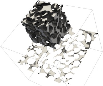
Three-dimensional (one eighth) sample of the pore space of the medium under investigation and a two-dimensional slice of it.

2 Pore-scale flow and transport
Flow and transport at the pore scale are governed by the following Stokes equation for the flow velocity
 $\boldsymbol{u}(\boldsymbol{x})$
and the advection–diffusion equation for the conservative scalar
 $c(\boldsymbol{x},t)$
:
 $$\begin{eqnarray}\displaystyle & \displaystyle \unicode[STIX]{x1D707}\unicode[STIX]{x1D6FB}^{2}\boldsymbol{u}(\boldsymbol{x})=\unicode[STIX]{x1D735}p(\boldsymbol{x}), & \displaystyle\end{eqnarray}$$
 $$\begin{eqnarray}\displaystyle & \displaystyle \frac{\unicode[STIX]{x2202}c(\boldsymbol{x},t)}{\unicode[STIX]{x2202}t}+\unicode[STIX]{x1D735}\boldsymbol{\cdot }\boldsymbol{u}(\boldsymbol{x},t)c(\boldsymbol{x},t)-D\unicode[STIX]{x1D6FB}^{2}c(\boldsymbol{x},t)=0, & \displaystyle\end{eqnarray}$$
where
 $\unicode[STIX]{x1D707}$
is the viscosity,
 $p(x)$
is pressure and
 $D$
is the molecular diffusion coefficient. These equations are solved numerically with the open-source finite-volume code OpenFOAM 4.x. Details about numerical discretisation and solvers are discussed in appendix A while boundary conditions and operating conditions are discussed below. We employ here a fully Eulerian formulation which, provided that an accurate discretisation and finite diffusion coefficient are used, is robust and has no statistical error.
2.1 Model medium
We consider the pore-scale sample described in Icardi et al. (Reference Icardi, Boccardo, Marchisio, Tosco and Sethi2014). As detailed in this study, the synthetic medium was generated according to the characteristics of standard sand samples. The grain size distribution was obtained from scanning electron microscopy and static-light scattering measurements and fitted by a Weibull probability density function (PDF) for the diameter of equivalent spheres,
 $$\begin{eqnarray}\displaystyle & \displaystyle p_{d}(d)=\frac{k}{d_{0}}\left(\frac{d}{d_{0}}\right)^{k-1}\text{e}^{-(d/d_{0})^{k}}. & \displaystyle\end{eqnarray}$$
The mean grain diameter is
 $\langle d\rangle =d_{0}\unicode[STIX]{x1D6E4}(1+1/k)=0.277~\text{mm}$
and the Weibull parameter is
 $k=7$
. This distribution is sharply peaked about its mean. The synthetic porous medium was generated by sampling grain sizes from the Weibull distribution (2.3) and sedimentation of irregularly shaped grains using the software package BLENDER, which resulted in a porosity of
 $n=0.35$
. It should be noted that the Weibull distribution (2.3) is a parametric PDF to represent the empirical grain size distribution. The lognormal PDF is another frequently used parameterisation for empirical grain size distributions (Friedman Reference Friedman1962). The model medium is cubic, of length
 $L=2~\text{mm}$
. It contains approximately
 $2\times 10^{3}$
grains. The characteristic pore length
 $\ell _{0}$
is of the order of the mean grain size,
 $\ell _{0}\approx \langle d\rangle =0.277~\text{mm}$
. The length
 $L$
of the study domain is
 $L=7.22\langle d\rangle$
. The volume is of the size of a representative elementary volume in terms of the definition of volumetric porosity (Bear Reference Bear1972). This means that in terms of this Darcy-scale property the medium can be considered to be macroscopically homogeneous. Figure 1 shows a section of the three-dimensional porous medium and a two-dimensional slice.
Uniform pressure boundary conditions are imposed at the inlet and the outlet, while zero-flux boundary conditions are imposed on the lateral boundaries. This results in a mean velocity
 $\langle \boldsymbol{u}(\boldsymbol{x})\rangle \equiv \langle u_{1}\rangle \boldsymbol{e}_{1}$
oriented towards the
 $1$
-axis with
 $\langle u_{1}\rangle =5.73\times 10^{-6}~\text{m}~\text{s}^{-1}$
and identifies the characteristic advection time
 $\unicode[STIX]{x1D70F}_{u}=L/\langle u_{1}\rangle$
. The Péclet number, which compares advective and diffusive transport over a pore length
 $\ell _{0}$
, is defined by
 $$\begin{eqnarray}\displaystyle & \displaystyle Pe=\frac{\langle u_{1}\rangle \ell _{0}}{D}. & \displaystyle\end{eqnarray}$$
2.2 Solute transport
Three-dimensional snapshots of the complementary residence concentration (
 $1-c(\boldsymbol{x},t)$
) concentration at approximately
 $t\approx 3\unicode[STIX]{x1D70F}_{u}$
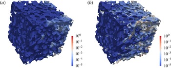
after a constant injection for a Péclet number of 30 (a) and 1000 (b). Flow is from left to right.

The solute transport (2.2) is solved in a fully Eulerian way. Different microscopic Péclet numbers, defined by (2.4), are imposed by tuning the molecular diffusion coefficient
 $D$
appropriately. It should be noted that
 $Pe$
is the only dimensionless group for the transport problem under consideration. Thus, varying the mean flow rate and varying the diffusion coefficient have the same effect as long as
 $Pe$
remains unchanged. No-flux boundary conditions are imposed at all boundaries except for the inlet where a constant concentration is assumed. Figure 2 shows snapshots of the concentration distribution in the pore space. We observe increasing spatial heterogeneity with increasing Péclet number. Specifically, for the high Péclet number, the invasion front is not homogeneous, with regions of low solute concentration next to regions of high concentration. This is an expression of local physical non-equilibrium, as discussed below.
Transport is characterised in terms of the complementary cumulative breakthrough curve, defined as
 $$\begin{eqnarray}\displaystyle & \displaystyle f(t)=1-\frac{\displaystyle \int \,\text{d}x_{2}\int \,\text{d}x_{3}c(x_{1}=L,x_{2},x_{4},t)u_{1}(x_{1}=L,x_{2},x_{3})}{\displaystyle \int \,\text{d}x_{2}\int \,\text{d}x_{3}u_{1}(x_{1}=L,x_{2},x_{3})}. & \displaystyle\end{eqnarray}$$
In the following, we refer to
 $f(t)$
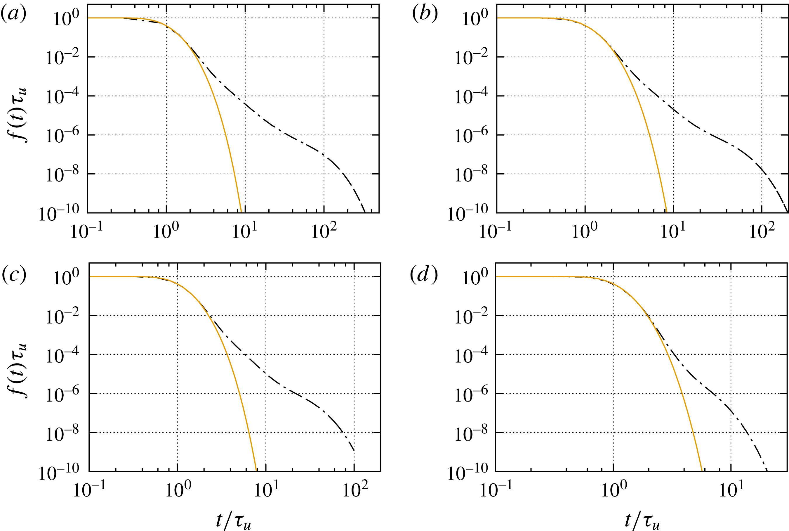
as the breakthrough curve. Figure 3 shows the solute breakthrough curves for different Péclet numbers. We observe increased tailing with increasing
 $Pe$
, in line with the snapshots of the concentration distribution shown in figure 2. Tailing of the breakthrough curves is an expression of local non-equilibrium because it is the result of a broad distribution of residence times in the sample.
Breakthrough curves for
 $Pe=10^{3}$
,
 $5\times 10^{2}$
,
 $3\times 10^{2}$
and
 $30$
. The dash-dotted lines in the following indicate the numerical data. The solid lines denote the solution (2.7) characterised by the dispersion coefficient
 ${\mathcal{D}}$
which is directly fitted from the breakthrough data.

In order to understand and interpret the breakthrough behaviour, we first consider the classical advection–dispersion approach. Icardi et al. (Reference Icardi, Boccardo, Marchisio, Tosco and Sethi2014) quantified the cumulative complementary breakthrough curves in the light of this approach, which characterises transport in terms of an advection–dispersion equation (ADE) for the evolution of the macroscale concentration
 $\overline{c}(x,t)$
(Hornung Reference Hornung1997; Whitaker Reference Whitaker1999),
 $$\begin{eqnarray}\displaystyle & \displaystyle \frac{\unicode[STIX]{x2202}\overline{c}(x,t)}{\unicode[STIX]{x2202}t}+\langle u_{1}\rangle \frac{\unicode[STIX]{x2202}\overline{c}(x,t)}{\unicode[STIX]{x2202}x}-{\mathcal{D}}\frac{\unicode[STIX]{x2202}^{2}\overline{c}(x,t)}{\unicode[STIX]{x2202}x^{2}}=0, & \displaystyle\end{eqnarray}$$
where
 ${\mathcal{D}}$
is the hydrodynamic dispersion coefficient. For simplicity in the following, we denote
 $x=x_{1}$
. Such a macroscale transport equation may be derived using volume averaging or homogenisation theory (Hornung Reference Hornung1997; Whitaker Reference Whitaker1999). It is a valid transport description if the support scale, the REV (Bear Reference Bear1972), is well mixed. Under well-mixed conditions, the macroscale concentration
 $\overline{c}(x,t)$
uniquely determines the concentration on the support scale at the position
 $x$
(Dentz et al.
Reference Dentz, Le Borgne, Lester and de Barros2016b
), which is not the case here for large
 $Pe$
. The solution for the complementary cumulative breakthrough curve
 $f(t,x)$
at a position
 $x$
in a semi-infinite medium is then given by (Kreft & Zuber Reference Kreft and Zuber1978)
 $$\begin{eqnarray}\displaystyle & \displaystyle f(t,x)=1-\frac{1}{2}\left[\text{erfc}\left(\frac{x-t}{\sqrt{4{\mathcal{D}}t}}\right)+\exp \left(\frac{x}{{\mathcal{D}}}\right)\text{erfc}\left({\displaystyle \frac{x+t}{\sqrt{4{\mathcal{D}}t}}}\right)\right]. & \displaystyle\end{eqnarray}$$
The latter is a good approximation to the solution for a finite domain for
 $Pe\gg 1$
, which is fulfilled for the scenarios of interest here. We denote
 $f(t)=f(t,x=L)$
. Figure 3 compares (2.7) with the numerical data for different values of
 $Pe$
. The onset and initial decay of the breakthrough curve are well represented by the mean flow velocity and a fitted dispersion coefficient
 ${\mathcal{D}}$
. However, it fails to capture the tailing behaviour at intermediate and long times. This implies that the system is not at local equilibrium and the support scale is not well mixed. In the following, we analyse these transport features and their origins in terms of spatial fluctuations of the pore-scale flow velocity and the effect of molecular diffusion. The aim is to gain understanding of the pore-scale transport mechanisms in order to arrive at a macroscale transport approach that can be quantified in terms of the pore-scale velocity, pore-size distributions and molecular diffusion. We first discuss the statistical properties of the Eulerian velocity and velocity magnitude in the light of the pore-size distribution before we analyse the mechanisms of pore-scale transport and their macroscale quantification in terms of
 $f(t)$
.
3 Eulerian velocity distributions and pore-scale velocity model
In order to understand the pore-scale dispersion behaviour, we study here the Eulerian velocity distribution and its interpretation in terms of the grain- and pore-size distribution. We consider the distribution of the velocity components in the mean flow direction,
 $u_{1}(\boldsymbol{x})$
, and perpendicular to it,
 $u_{i}(\boldsymbol{x})$
for
 $i\neq 1$
, as well as the velocity magnitude
 $v_{e}(\boldsymbol{x})=\sqrt{\sum _{i}u_{i}(\boldsymbol{x})^{2}}$
. The Eulerian velocity PDFs are computed as volume weighted histograms over the entire pore space
 $\unicode[STIX]{x1D714}$
,
 $$\begin{eqnarray}\displaystyle & \displaystyle p_{e}(v)=\frac{1}{V_{\unicode[STIX]{x1D714}}}\int _{\unicode[STIX]{x1D714}}\,\text{d}\boldsymbol{x}\unicode[STIX]{x1D6FF}[v-v(\boldsymbol{x})], & \displaystyle\end{eqnarray}$$
where
 $V_{\unicode[STIX]{x1D714}}$
is the pore volume;
 $v(\boldsymbol{x})=u_{i}(\boldsymbol{x})$
for the PDF of velocity components and
 $v(\boldsymbol{x})=v_{e}(\boldsymbol{x})$
for the PDF of the velocity magnitude. It should be noted that these PDFs generally depend on the sampling volume. For the sand-like porous medium under consideration here, the sampling volume is of the size of an REV; thus, the velocity PDF is assumed not to change significantly on increasing the sampling volume.
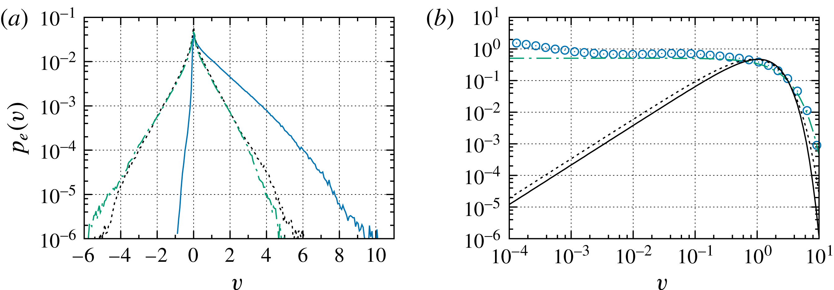
The PDFs of the velocity components are shown in figure 4. The distributions of the components perpendicular to the mean flow direction are symmetric around
 $0$
and have an exponential shape. The PDF of the longitudinal component is skewed towards positive values with an approximately stretched exponential shape (Siena et al.
Reference Siena, Riva, Hyman, Winter and Guadagnini2014; Holzner et al.
Reference Holzner, Morales, Willmann and Dentz2015). It is non-zero for small negative velocities, which indicates the presence of backflow. It is not clear how to relate the distributions of the velocity components to statistical characteristics of the porous medium.
(a) The PDFs of (solid)
 $u_{1}(\boldsymbol{x})$
, (dashed)
 $u_{2}(\boldsymbol{x})$
and (dash-dotted)
 $u_{3}(\boldsymbol{x})$
. (b) The PDFs of the magnitude of Eulerian velocities (circles) and estimation with the velocity model (3.10) for
 $v_{0}=2.1\langle u_{1}\rangle$
and
 $\unicode[STIX]{x1D6FC}=2.5$
(dash-dotted). The solid line denotes the PDF (3.14) of mean pore velocities and the dashed line its approximation by (3.16). Velocities are normalised by
 $\langle u_{1}\rangle$
.

In order to relate the medium properties to the Eulerian flow field, we focus rather on the PDF of velocity magnitudes illustrated in figure 4. The PDF is flat from
 $10^{-3}$
to
 $1$
, from where on it decays exponentially rapidly. As detailed below, the flat distribution at small velocities can be understood by sampling a parabolic velocity profile; the smooth cutoff at larger velocities may be related to the distribution of pore sizes. The deviation from the flat profile at small velocities may be attributed to low-velocity zones in the wake of solid grains, as discussed in § 4.2.
First, we consider the mean of the Eulerian velocity magnitude. It is related to the mean velocity through the advective tortuosity
 $\unicode[STIX]{x1D712}$
as (Koponen, Kataja & Timonen Reference Koponen, Kataja and Timonen1996)
 $$\begin{eqnarray}\displaystyle & \displaystyle \langle v_{e}\rangle =\unicode[STIX]{x1D712}\langle u_{1}\rangle . & \displaystyle\end{eqnarray}$$
The advective tortuosity measures the ratio of average trajectory length to linear distance. For the model medium under consideration, the mean flow velocity is
 $\langle u_{1}\rangle =5.7\times 10^{-6}~\text{m}~\text{s}^{-1}$
and the mean velocity magnitude is
 $\langle v_{e}\rangle =9\times 10^{-6}~\text{m}~\text{s}^{-1}$
. Thus, the tortuosity is given by
 $\unicode[STIX]{x1D712}=\langle v_{e}\rangle /\langle u_{1}\rangle =1.6$
.
The velocity profile across the porous medium perpendicular to the main flow direction.

In the following, we study the PDF of velocity magnitudes based on the assumption that the velocity profile in a single pore is parabolic (Saffman Reference Saffman1959; Lester, Metcalfe & Trefry Reference Lester, Metcalfe and Trefry2013; Holzner et al. Reference Holzner, Morales, Willmann and Dentz2015; De Anna et al. Reference De Anna, Quaife, Biros and Juanes2017). The validity of this assumption is underlined qualitatively by the velocity profiles shown in figure 5, which are obtained along a cut of the three-dimensional porous medium of figure 2. It should be noted that some authors (Le Borgne et al. Reference Le Borgne, Bolster, Dentz, de Anna and Tartakovsky2011) have studied flow and transport in wavy tubes representing a serial arrangement of pores, as a model system for the upscaling of pore-scale heterogeneity. This view is not appropriate for more complex porous media, for which the network aspect is important in the sense that pore intersections exist such that the concept of the linear pore breaks down. Some aspects of flow in serial and parallel pore arrangements are discussed in Holzner et al. (Reference Holzner, Morales, Willmann and Dentz2015).
The PDF (3.1) of the velocity magnitude can be decomposed into the contributions from the individual pores as
 $$\begin{eqnarray}\displaystyle & \displaystyle p_{e}(v)=\mathop{\sum }_{p}\frac{V_{p}}{V_{\unicode[STIX]{x1D714}}}\frac{1}{V_{p}}\int _{\unicode[STIX]{x1D714}_{p}}\,\text{d}\boldsymbol{x}\unicode[STIX]{x1D6FF}[v-v(\boldsymbol{x})], & \displaystyle\end{eqnarray}$$
where
 $\unicode[STIX]{x1D714}_{p}$
is the single pore domain and
 $V_{p}$
its volume. The velocity
 $v(\boldsymbol{x})\equiv v(r)$
depends only on the pore radius and is given by
 $$\begin{eqnarray}\displaystyle & \displaystyle v(r)=v_{p}\left[1-\left(\frac{2r}{a_{p}}\right)^{2}\right], & \displaystyle\end{eqnarray}$$
where
 $a_{p}$
is the pore diameter and
 $r$
is the distance from the pore axis. The maximum velocity
 $v_{p}$
in a pore is given by
 $v_{p}=v_{0}(a_{p}/a_{0})^{2}$
, with
 $v_{0}$
a characteristic velocity and
 $a_{0}$
a characteristic pore diameter. Under this assumption, we obtain
 $$\begin{eqnarray}\displaystyle & \displaystyle p_{e}(v)=\mathop{\sum }_{p}\frac{V_{p}}{V_{\unicode[STIX]{x1D714}}}\frac{1}{v_{p}}H(v_{p}-v), & \displaystyle\end{eqnarray}$$
where
 $H(v)$
denotes the Heaviside step function. It should be noted that the velocity PDF in a single pore is uniform between
 $0$
and the maximum velocity
 $v_{p}$
, which can be seen by sampling
 $v(r)$
given by (3.4) uniformly in a pore cross-section.
We furthermore assume that the pore volume is
 $V_{p}=ba_{p}^{2}\ell _{p}$
, with
 $b$
a shape factor,
 $\ell _{p}$
the pore length and
 $a_{p}$
the pore diameter. In the following, we assume that the pore length
 $\ell _{p}\approx \ell _{0}$
is approximately constant, while the pore diameter
 $a_{p}$
is variable. For the sand-like medium under consideration, the pore length is of the order of the grain size. As the grain size distribution (2.3) is sharply peaked, we approximate it as constant. The pore diameter, in contrast, depends on the distance of the grains in the packing, which is much more variable. This is indicated in the two-dimensional slice of the porous medium shown in figure 1. We can now write
 $$\begin{eqnarray}\displaystyle & \displaystyle p_{e}(v)=\mathop{\sum }_{p}\frac{ba_{0}^{2}\ell _{0}}{V_{\unicode[STIX]{x1D714}}}\frac{1}{v_{0}}H[v_{0}(a_{p}/a_{0})^{2}-v]. & \displaystyle\end{eqnarray}$$
This expression can be written tautologically as
 $$\begin{eqnarray}\displaystyle & \displaystyle p_{e}(v)=\int \,\text{d}a\frac{ba_{0}^{2}\ell _{0}N_{0}}{V_{\unicode[STIX]{x1D714}}}\frac{1}{v_{0}}H[v_{0}(a/a_{0})^{2}-v]\left[\frac{1}{N_{0}}\mathop{\sum }_{p}\unicode[STIX]{x1D6FF}(a-a_{p})\right], & \displaystyle\end{eqnarray}$$
where
 $N_{0}$
is the number of pores. We note that the expression in square brackets on the right-hand side is equal to the PDF of pore diameters
 $p_{a}(a)$
, and define the average volume of a single pore as
 $\langle V_{p}\rangle =V_{\unicode[STIX]{x1D714}}/N_{0}$
. Thus, (3.7) can be written as
 $$\begin{eqnarray}\displaystyle & \displaystyle p_{e}(v)=\int \,\text{d}a\frac{ba_{0}^{2}\ell _{0}}{\langle V_{p}\rangle }\frac{1}{v_{0}}H[v_{0}(a/a_{0})^{2}-v]p_{a}(a). & \displaystyle\end{eqnarray}$$
The grain size distribution is given by a Weibull distribution. We assume for the pore-size distribution also a Weibull distribution, with
 $$\begin{eqnarray}\displaystyle & \displaystyle p_{a}(a)=\frac{\unicode[STIX]{x1D6FC}}{a_{0}}\left(\frac{a}{a_{0}}\right)^{\unicode[STIX]{x1D6FC}-1}\exp [-(a/a_{0})^{\unicode[STIX]{x1D6FC}}]. & \displaystyle\end{eqnarray}$$
We note that the average pore volume is
 $\langle V_{p}\rangle \propto a_{0}^{2}\ell _{0}$
. Using these relations in (3.8), we obtain after integration and normalisation the following estimation for the Eulerian velocity PDF:
 $$\begin{eqnarray}\displaystyle & \displaystyle p_{e}(v)=\frac{\exp \left[-(v/v_{0})^{\unicode[STIX]{x1D6FC}/2}\right]}{v_{0}\unicode[STIX]{x1D6E4}(1+2/\unicode[STIX]{x1D6FC})}. & \displaystyle\end{eqnarray}$$
The mean velocity is given by
 $$\begin{eqnarray}\displaystyle & \displaystyle \langle v_{e}\rangle =v_{0}\frac{\unicode[STIX]{x1D6E4}(4/\unicode[STIX]{x1D6FC})}{\unicode[STIX]{x1D6E4}(2/\unicode[STIX]{x1D6FC})}. & \displaystyle\end{eqnarray}$$
By fitting the Eulerian velocity data, we estimate an exponent of
 $\unicode[STIX]{x1D6FC}\approx 2.5$
and
 $v_{0}\approx 2.1\langle u_{1}\rangle$
, which has the same average velocity of
 $\langle v_{e}\rangle =1.6\langle u_{1}\rangle$
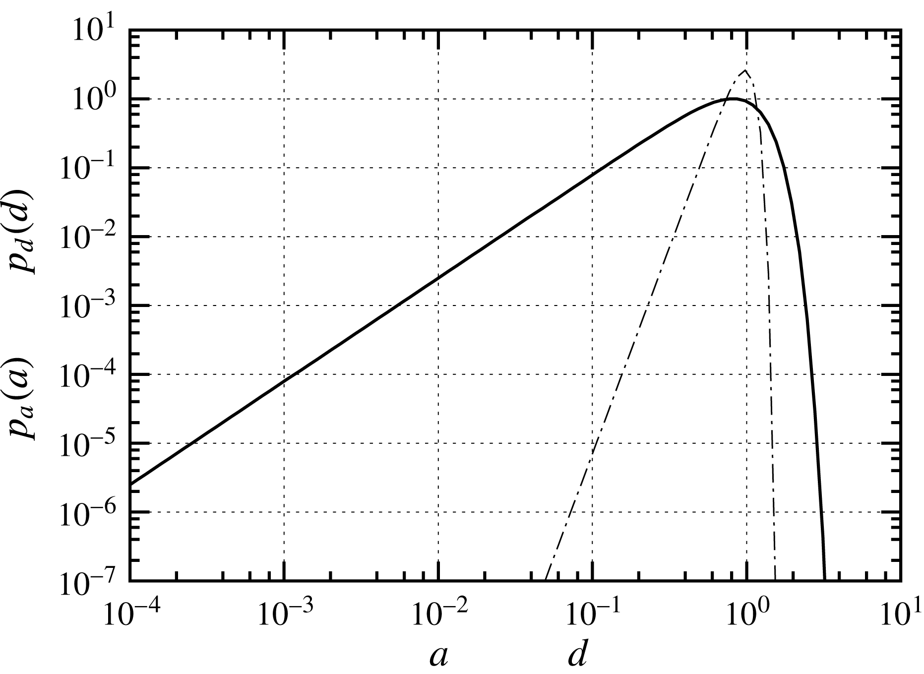
as the data. The proposed velocity model implies that the PDF of pore diameters can be characterised by a Weibull distribution with
 $\unicode[STIX]{x1D6FC}=2.5$
. Figure 6 shows the grain size PDF
 $p_{d}(d)$
of grain diameters and the PDF of pore diameters
 $p_{a}(a)$
estimated from the above velocity model. The distribution of pore diameters is much more variable than the grain size distribution, specifically towards low values. This is intuitive because the pore size is related to the distance between grains in the packings, which can be much smaller than the grain size; see also figure 1.


From the PDF of pore diameters, we can estimate the PDF of mean velocities,
 $v_{m}=v_{p}/2$
, which is
 $$\begin{eqnarray}\displaystyle & \displaystyle p_{m}(v)=\int \,\text{d}a\frac{ba^{2}\ell _{0}}{\langle V_{p}\rangle }\unicode[STIX]{x1D6FF}[v_{0}(a/a_{0})^{2}/2-v]p_{a}(a). & \displaystyle\end{eqnarray}$$
By setting again
 $\langle V_{p}\rangle \propto a_{0}^{2}\ell _{0}$
and using the Weibull distribution (3.9), we obtain
 $$\begin{eqnarray}\displaystyle & \displaystyle p_{m}(v)\propto \frac{1}{v_{0}}\int \,\text{d}a\unicode[STIX]{x1D6FF}(a^{2}-2v/v_{0})\unicode[STIX]{x1D6FC}a^{\unicode[STIX]{x1D6FC}+1}\exp [-a^{\unicode[STIX]{x1D6FC}}]. & \displaystyle\end{eqnarray}$$
By evaluating the Dirac delta and normalising, we obtain
 $$\begin{eqnarray}\displaystyle & \displaystyle p_{m}(v)=\frac{\unicode[STIX]{x1D6FC}}{v_{0}\unicode[STIX]{x1D6E4}(1+2/\unicode[STIX]{x1D6FC})}\left(\frac{2v}{v_{0}}\right)^{\unicode[STIX]{x1D6FC}/2}\exp \left[-\left(\frac{2v}{v_{0}}\right)^{\unicode[STIX]{x1D6FC}/2}\right]. & \displaystyle\end{eqnarray}$$
We thus obtain for the average of
 $v_{m}$
 $$\begin{eqnarray}\displaystyle & \displaystyle \langle v_{m}\rangle =v_{0}\frac{\unicode[STIX]{x1D6E4}(1+4/\unicode[STIX]{x1D6FC})}{2\unicode[STIX]{x1D6E4}(1+2/\unicode[STIX]{x1D6FC})}=v_{0}\frac{\unicode[STIX]{x1D6E4}(4/\unicode[STIX]{x1D6FC})}{\unicode[STIX]{x1D6E4}(2/\unicode[STIX]{x1D6FC})}\equiv \langle v_{e}\rangle . & \displaystyle\end{eqnarray}$$
Expression (3.14) implies that
 $p_{m}(v)\propto v^{a-1}$
, with
 $a=\unicode[STIX]{x1D6FC}/2+1$
. The PDF of the mean velocities is characterised by lower weights than the Eulerian PDF on both low and high velocities. This is illustrated in figure 4. We approximate (3.14) in the following by the
 $\unicode[STIX]{x1D6E4}$
distribution
 $$\begin{eqnarray}\displaystyle & \displaystyle p_{m}(v)=\frac{1}{v_{\unicode[STIX]{x1D6FE}}\unicode[STIX]{x1D6E4}(a)}\left(\frac{v}{v_{\unicode[STIX]{x1D6FE}}}\right)^{a-1}\exp \left(-\frac{v}{v_{\unicode[STIX]{x1D6FE}}}\right), & \displaystyle\end{eqnarray}$$
where
 $a=\unicode[STIX]{x1D6FC}/2+1$
and
 $v_{\unicode[STIX]{x1D6FE}}=\langle v_{e}\rangle /a$
. The quality of this approximation is shown in figure 4. As we will see in the following, the PDF of mean velocities plays an important role for the interpretation of solute dispersion under finite Péclet numbers.
4 Pore-scale transport mechanisms and upscaling
We study the pore-scale transport mechanisms in the light of heterogeneous advection and diffusion in the pore space. As discussed above, pore-scale transport mechanisms have been characterised by advection–dispersion models in terms of the average pore velocity
 $\langle u_{1}\rangle$
and effective dispersion coefficients
 ${\mathcal{D}}$
(e.g. Bijeljic, Muggeridge & Blunt Reference Bijeljic, Muggeridge and Blunt2004; Scheven, Harris & Johns Reference Scheven, Harris and Johns2007; Icardi et al.
Reference Icardi, Boccardo, Marchisio, Tosco and Sethi2014), and dual domain models (Liu & Kitanidis Reference Liu and Kitanidis2012; Gjetvaj et al.
Reference Gjetvaj, Russian, Gouze and Dentz2015) to capture the impact of diffusion into the immobile porosity and low-velocity regions. The impact of advective heterogeneity has been studied in the framework of continuous time and time-domain random walks (Bijeljic & Blunt Reference Bijeljic and Blunt2006; Bijeljic et al.
Reference Bijeljic, Mostaghimi and Blunt2011; Le Borgne et al.
Reference Le Borgne, Bolster, Dentz, de Anna and Tartakovsky2011; De Anna et al.
Reference De Anna, Le Borgne, Dentz, Tartakovsky, Bolster and Davy2013; Kang et al.
Reference Kang, de Anna, Nunes, Bijeljic, Blunt and Juanes2014; Gjetvaj et al.
Reference Gjetvaj, Russian, Gouze and Dentz2015; Holzner et al.
Reference Holzner, Morales, Willmann and Dentz2015). Here, we analyse in detail the interplay of heterogeneous advection from the intra- to the interpore scale and diffusion in order to identify and quantify the dominant transport mechanisms.
To this end, we model solute transport in a particle-based framework through spatial transitions over the characteristic pore length
 $\ell \sim \ell _{0}$
with a (variable) duration
 $\unicode[STIX]{x1D70F}$
(Saffman Reference Saffman1959). In this picture, the position
 $x_{n}$
and time
 $t_{n}$
of a solute particle along the mean flow direction are given after
 $n$
steps as
 $$\begin{eqnarray}\displaystyle & \displaystyle x_{n+1}=x_{n}+\unicode[STIX]{x1D709}_{n},\quad t_{n+1}=t_{n}+\unicode[STIX]{x1D70F}_{n}. & \displaystyle\end{eqnarray}$$
The spatial step
 $\unicode[STIX]{x1D709}_{n}$
may be downstream or upstream depending on the local advection and diffusion conditions. The transition length is given by
 $|\unicode[STIX]{x1D709}_{n}|=\ell /\unicode[STIX]{x1D712}$
. Particles make transitions along their trajectory of length
 $\ell$
. The random walk (4.1), however, describes transport along the mean flow direction. Thus, the transition length is corrected by the advective tortuosity
 $\unicode[STIX]{x1D712}$
, which accounts for the fact that particle trajectories through the pore space are not straight. The transition time
 $\unicode[STIX]{x1D70F}_{n}$
depends on the pore-scale advection and diffusion mechanisms as discussed in detail below and illustrated schematically in figure 7. We assume that the advection and diffusion properties at subsequent positions are statistically independent, which implies that the
 $\unicode[STIX]{x1D70F}_{n}$
are identical independent random variables. This is a reasonable assumption because flow and particle velocities are only weakly correlated between pores (Saffman Reference Saffman1959; Bijeljic et al.
Reference Bijeljic, Mostaghimi and Blunt2011; Le Borgne et al.
Reference Le Borgne, Bolster, Dentz, de Anna and Tartakovsky2011; De Anna et al.
Reference De Anna, Le Borgne, Dentz, Tartakovsky, Bolster and Davy2013; Lester et al.
Reference Lester, Metcalfe and Trefry2013; Kang et al.
Reference Kang, de Anna, Nunes, Bijeljic, Blunt and Juanes2014; Holzner et al.
Reference Holzner, Morales, Willmann and Dentz2015).
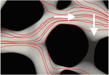
Schematic of transitions in the time-domain random walk model (4.1). The thin red lines represent streamlines of the flow in a cross-section of the porous medium. The shading of the background denotes the absolute value of the flow velocity, which decreases from light to dark; black areas denote the grains. The horizontal arrow denotes particle transitions over the length of a pore in the streamwise direction and the vertical arrow indicates particle transitions across streamlines into low-velocity zones in the wake of the solid grains. Transitions along streamlines are due to mean advection in the pore and diffusion. Transitions across the streamlines are due to diffusion. Particles that enter the immobile zones remain there for the residence time
 $\unicode[STIX]{x1D70F}_{f}$
before they are released back into the mobile portion of the medium.

Equation (4.1) describes a time-domain random walk (TDRW) (Cvetkovic et al.
Reference Cvetkovic, Dagan and Shapiro1991; Delay, Ackerer & Danquigny Reference Delay, Ackerer and Danquigny2005; Painter & Cvetkovic Reference Painter and Cvetkovic2005; Noetinger et al.
Reference Noetinger, Roubinet, Russian, Le Borgne, Delay, Dentz, De Dreuzy and Gouze2016; Russian, Dentz & Gouze Reference Russian, Dentz and Gouze2016) or equivalently a continuous time random walk (CTRW) (Montroll & Weiss Reference Montroll and Weiss1965; Scher & Lax Reference Scher and Lax1973; Berkowitz et al.
Reference Berkowitz, Cortis, Dentz and Scher2006). It is characterised by the joint PDF of transition length
 $\unicode[STIX]{x1D709}$
and time
 $\unicode[STIX]{x1D70F}$
, denoted by
 $\unicode[STIX]{x1D713}(x,t)$
, which encodes the pore-scale transport mechanisms. The marginal PDF of transition times is defined by
 $$\begin{eqnarray}\displaystyle & \displaystyle \unicode[STIX]{x1D713}(t)=\int \,\text{d}x\unicode[STIX]{x1D713}(x,t). & \displaystyle\end{eqnarray}$$
The evolution of the macroscale solute concentration in this framework is given by the generalised master equation (Kenkre, Montroll & Shlesinger Reference Kenkre, Montroll and Shlesinger1973; Berkowitz et al. Reference Berkowitz, Cortis, Dentz and Scher2006; Comolli et al. Reference Comolli, Hidalgo, Moussey and Dentz2016)
 $$\begin{eqnarray}\displaystyle & \displaystyle \frac{\unicode[STIX]{x2202}\overline{c}(x,t)}{\unicode[STIX]{x2202}t}=\int \,\text{d}x^{\prime }\int _{0}^{t}\,\text{d}t^{\prime }{\mathcal{K}}(x-x^{\prime },t-t^{\prime })\left[\overline{c}(x^{\prime },t^{\prime })-\overline{c}(x,t^{\prime })\right]. & \displaystyle\end{eqnarray}$$
It expresses the fact that the change of solute concentration at a given position depends on the transport history and in this sense accounts for incomplete mixing, or non-uniqueness of concentration on the support scale. The macroscale concentration at a given position is composed of solute particles with different transport histories, which is quantified by the distribution of transition times. The memory kernel
 ${\mathcal{K}}(x,t)$
denotes the probability per time of a particle transition of length
 $x-x^{\prime }$
during time
 $t-t^{\prime }$
. It relates solute fluxes at earlier times
 $t^{\prime }<t$
to concentration changes at time
 $t$
. Under Markovian conditions, the change of the solute concentration is only determined by the local in time solute fluxes. The memory kernel is given in terms of the distribution of transition length and times. It is defined through its Laplace transform as
 $$\begin{eqnarray}\displaystyle & \displaystyle {\mathcal{K}}^{\ast }(x,\unicode[STIX]{x1D706})=\frac{\unicode[STIX]{x1D706}\unicode[STIX]{x1D713}^{\ast }(x,\unicode[STIX]{x1D706})}{1-\unicode[STIX]{x1D713}^{\ast }(\unicode[STIX]{x1D706})}. & \displaystyle\end{eqnarray}$$
The Laplace transform is defined in Abramowitz & Stegun (Reference Abramowitz and Stegun1972); Laplace transformed quantities are marked by an asterisk and the Laplace variable is denoted by
 $\unicode[STIX]{x1D706}$
. If the kernel
 ${\mathcal{K}}(x,t)$
is short range in
 $x$
, meaning that it decays sufficiently fast for
 $|x|$
larger than a characteristic length scale, (4.3) can be localised in space (Berkowitz et al.
Reference Berkowitz, Klafter, Metzler and Scher2002; Dentz et al.
Reference Dentz, Cortis, Scher and Berkowitz2004),
 $$\begin{eqnarray}\displaystyle \frac{\unicode[STIX]{x2202}\overline{c}(x,t)}{\unicode[STIX]{x2202}t}+\int _{0}^{t}\,\text{d}t^{\prime }\left[\unicode[STIX]{x1D708}(t-t^{\prime })\frac{\unicode[STIX]{x2202}\overline{c}(x,t^{\prime })}{\unicode[STIX]{x2202}x}-\unicode[STIX]{x1D705}(t-t^{\prime })\frac{\unicode[STIX]{x2202}^{2}\overline{c}(x,t^{\prime })}{\unicode[STIX]{x2202}x^{2}}\right]=0. & & \displaystyle\end{eqnarray}$$
The drift and diffusion kernels are defined by
 $$\begin{eqnarray}\displaystyle \unicode[STIX]{x1D708}(t)=\int \,\text{d}xx{\mathcal{K}}(x,t), & & \displaystyle\end{eqnarray}$$
 $$\begin{eqnarray}\displaystyle \unicode[STIX]{x1D705}(t)=\frac{1}{2}\int \,\text{d}xx^{2}{\mathcal{K}}(x,t). & & \displaystyle\end{eqnarray}$$
In the following, we solve for the macroscale transport behaviour using random walk particle tracking simulations based on (4.1). The solute arrival time at a position
 $x$
is thus given by (Comolli et al.
Reference Comolli, Hidalgo, Moussey and Dentz2016)
 $$\begin{eqnarray}\displaystyle & \displaystyle \unicode[STIX]{x1D70F}_{a}(x)=t_{n_{a}(x)},\quad n_{a}(x)=\inf (n|x_{n}\geqslant x), & \displaystyle\end{eqnarray}$$
where
 $n_{a}(x)$
is the number of steps a particle requires to arrive at the outlet. The distribution of arrival times, denoted by
 $p_{a}(t,x)$
, is defined by
 $$\begin{eqnarray}\displaystyle & \displaystyle p_{a}(t,x)=\langle \unicode[STIX]{x1D6FF}[t-\unicode[STIX]{x1D70F}_{a}(x)]\rangle . & \displaystyle\end{eqnarray}$$
The complementary cumulative breakthrough curve, or in the following only breakthrough curve, is thus given by
 $$\begin{eqnarray}\displaystyle & \displaystyle f(t,x)=\int _{t}^{\infty }\,\text{d}t^{\prime }p_{a}(t^{\prime },x)=\langle H[\unicode[STIX]{x1D70F}_{a}(x)-t]\rangle , & \displaystyle\end{eqnarray}$$
where
 $H(t)$
is the Heaviside step function. Expression (4.9) is the probability that the arrival time is larger than
 $t$
. In the following, we denote the breakthrough curve at the outlet at
 $x=L$
by
 $f(t)\equiv f(t,x=L)$
.
Equation (4.1) for the particle motion and its counterpart (4.3) for the particle distribution describe the non-local evolution of macroscale concentration due to local physical non-equilibrium, but are not predictive as long as
 $\unicode[STIX]{x1D713}(x,t)$
is not known. However, the TDRW approach provides a framework to identify and quantify the dominant pore-scale transport mechanisms in terms of the distribution of the Eulerian flow velocity and the diffusion properties in the medium. Thus, in the following, we investigate the structure of
 $\unicode[STIX]{x1D713}(x,t)$
in the light of the dominant pore-scale transport mechanisms and their manifestations on large-scale transport.
Figure 7 shows a schematic of possible particle transitions. Solute particles move along the pores due to advection–diffusion and may access low-velocity regions in the wake of the grains by diffusion only. We first consider the impact of heterogeneous advection and diffusion along streamlines on the behaviour of the arrival time distribution. Then, we study the influence of diffusion across streamlines into low-velocity zones and its quantification. Finally, we consider the combined impact of advective heterogeneity and diffusion along and across pores on large-scale transport.
4.1 Heterogeneous advection and diffusion
We analyse here the role of heterogeneous advection and diffusion along the streamlines within and between pores. To this end, we first consider purely advective particle motion and the resulting large-scale transport behaviour in terms of the particle arrival time distributions. Then, we analyse the effect of diffusion first on the intrapore and then on the interpore particle motion.
4.1.1 Pure advection
For infinite
 $Pe$
, i.e., purely advective transport, (4.1) becomes
 $$\begin{eqnarray}\displaystyle & \displaystyle x_{n+1}=x_{n}+\frac{\ell }{\unicode[STIX]{x1D712}},\quad t_{n+1}=t_{n}+\frac{\ell }{v_{n}}. & \displaystyle\end{eqnarray}$$
Particles move only forward along streamlines and the transition times
 $\unicode[STIX]{x1D70F}_{n}=\ell /v_{n}$
denote the advection time over the distance
 $\ell$
by the velocity magnitude
 $v_{n}$
. The magnitudes
 $v_{n}$
of particle velocities are distributed according to the streamwise velocity PDF
 $p_{s}(v)$
defined as follows. First, we note that the TDRW (4.1) samples particle velocities equidistantly along trajectories, while the Eulerian velocity PDF is sampled volumetrically in space. For divergence-free flow,
 $p_{s}(v)$
is related to the Eulerian velocity PDF through flux weighting (Saffman Reference Saffman1959; Dentz et al.
Reference Dentz, Kang, Comolli, Le Borgne and Lester2016a
; Comolli & Dentz Reference Comolli and Dentz2017),
 $$\begin{eqnarray}\displaystyle & \displaystyle p_{s}(v)=\frac{vp_{e}(v)}{\langle v_{e}\rangle }. & \displaystyle\end{eqnarray}$$
This relation can be understood qualitatively by noting that low flow velocities occupy wider streamtubes than high velocities because of fluid volume conservation. Thus, volumetric sampling emphasises low flow velocities. Equidistant velocity sampling along streamlines, on the other hand, weighs high and low velocities equally. This difference in sampling between the Eulerian and streamwise velocity distributions is compensated in (4.11) through flux weighting.
With this relation, the PDF of purely advective transition times, denoted here by
 $\unicode[STIX]{x1D713}_{a}(t)$
, can be directly related to the distribution
 $\unicode[STIX]{x1D713}_{a}(t)$
of advective transition times as
 $$\begin{eqnarray}\displaystyle & \displaystyle \unicode[STIX]{x1D713}_{a}(t)=\frac{\ell }{t^{3}\langle v_{e}\rangle }p_{e}(\ell /t). & \displaystyle\end{eqnarray}$$
The Eulerian PDF
 $p_{e}(v)$
goes towards a constant at small velocities and is cut off as a stretched exponential at large velocities; see figure 4 and (3.10). For the numerical implementation of the TDRW, we approximate the Eulerian velocity PDF (3.10) by an exponential distribution characterised by the same mean velocity. Specifically, the characteristic that determines the late-time behaviour of the breakthrough curve is the behaviour of
 $p_{e}(v)$
at small velocities
 $v\ll \langle v_{e}\rangle$
, for which it is constant. Thus, from (4.12), we obtain that the PDF of transition times behaves as
 $\unicode[STIX]{x1D713}_{a}(t)\propto t^{-1-b}$
, with
 $b=2$
for times
 $t\gg \unicode[STIX]{x1D70F}_{u}$
. Thus,
 $\unicode[STIX]{x1D713}_{a}(t)$
is an asymptotically stable distribution.
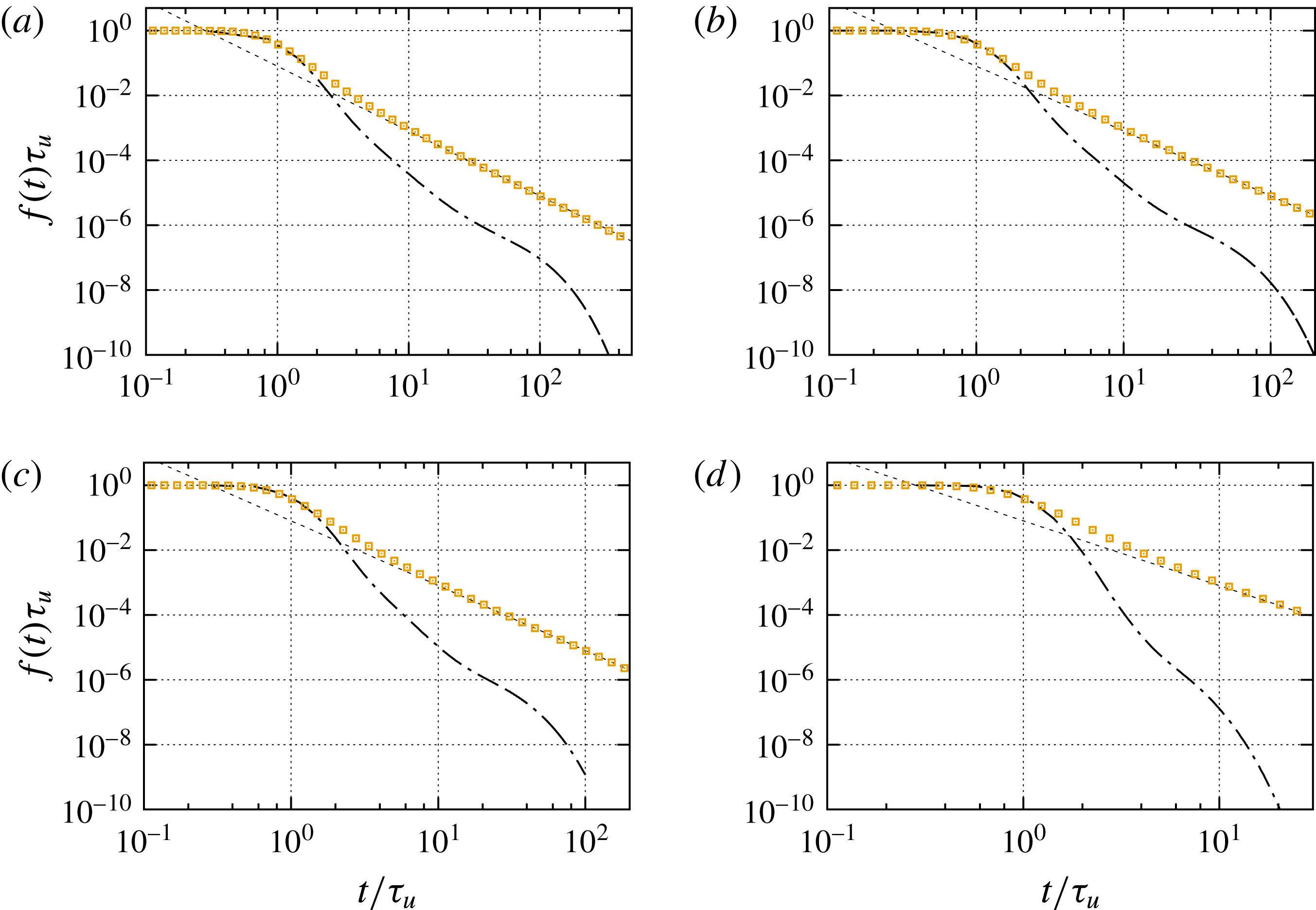
Breakthrough curves for
 $Pe=10^{3}$
,
 $5\times 10^{2}$
,
 $3\times 10^{2}$
and
 $30$
. The symbols denote the breakthrough curves obtained from the TDRW (4.10) based on purely advective transport,
 $Pe=\infty$
, for the transition length
 $\ell \approx 0.84\ell _{p}$
. The dashed lines show the predicted
 $t^{-2}$
scaling. The TDRW simulations use
 $10^{9}$
particles.

The breakthrough or arrival times at the outlet are given by
 $$\begin{eqnarray}\displaystyle & \displaystyle \unicode[STIX]{x1D70F}_{a}=\mathop{\sum }_{i=1}^{n_{a}}\unicode[STIX]{x1D70F}_{i}, & \displaystyle\end{eqnarray}$$
where the number of steps
 $n_{a}=\lceil L\unicode[STIX]{x1D712}/\ell \rceil$
, where
 $\lceil \cdot \rceil$
is the ceiling function. As
 $\unicode[STIX]{x1D713}_{a}(t)$
is stable, the PDF of arrival times, as a sum of stable random variables, has the same long-time behaviour as
 $p_{f}(t,x)\propto t^{-1-b}$
. Thus, the breakthrough curve is
 $f(t,x)\propto t^{-b}$
; see (4.9). This means here that the breakthrough curve is predicted to behave as
 $f(t)\propto t^{-2}$
. Figure 8 compares the numerically obtained breakthrough curves for different Péclet numbers with the predictions of (4.10) parameterised by the advective transition time PDF (4.12). The purely advective breakthrough curve is of course independent of
 $Pe$
and shows the
 $t^{-2}$
decay, as predicted. Moreover, here, the onset and initial decay of the breakthrough curves are well captured, but the purely advective model fails to represent the tails of the pore-scale data. It overestimates the tailing, while the ADE model underestimates it.
For all values of
 $Pe$
, we observe two distinct tailing behaviours, namely an intermediate tail whose decay is slower than the exponential tail predicted by the ADE and a flatter long-time tail that is cut off exponentially. The slope of the intermediate tail and the onset and final decay of the late-time tail clearly depend on the Péclet number and thus on diffusion. In the following, we study these mechanisms in more detail.
4.1.2 Advection under diffusion
Diffusion acts on how particles experience the flow velocities in two ways. First, within a pore, diffusion enables particles to sample the flow profile across the pore (Saffman Reference Saffman1959; Haber & Mauri Reference Haber and Mauri1988; Dentz & Carrera Reference Dentz and Carrera2007). This implies that the effective velocity experienced by a particle along a pore tends towards the mean velocity
 $v_{m}$
. The velocity extremes are attenuated by diffusion. It is these extremes, particularly the low velocities close to the pore walls, that cause the
 $t^{-2}$
tails predicted by the purely advective model. If the diffusion time across the pore is smaller than the characteristic advection time along the pore, particles move effectively with the mean velocity
 $v_{m}$
(Saffman Reference Saffman1959). This is a good approximation here because the estimated distribution of pore diameters is much broader than the distribution of pore lengths, and tailed towards small values, as shown in figure 6. This means that the transport relevant velocity distribution is the PDF of mean pore velocities (3.14) rather than the PDF (3.10) of point-wise velocities. It should be noted that the mean pore velocities are still sampled volumetrically, while the particle velocities are sampled spatially along streamlines. Thus, as outlined above, the distribution of particle velocities is given by flux weighting of
 $p_{m}(v)$
as
 $$\begin{eqnarray}\displaystyle & \displaystyle p_{s}(v)=\frac{vp_{m}(v)}{\langle v_{e}\rangle }, & \displaystyle\end{eqnarray}$$
where, it should be recalled that
 $\langle v_{m}\rangle =\langle v_{e}\rangle$
.
The transition time over the pore length is the result of advection by the mean pore velocity and diffusion. For example, for pores whose advection time
 $\ell /v_{m}$
is larger than the diffusion time
 $\ell ^{2}/2D$
along the pore, the particle transition time is dominated by diffusion. The transition time is limited by the characteristic diffusion time (Saffman Reference Saffman1959). The distribution of advective–diffusive transit times over a given distance can be seen as a first-passage problem (Redner Reference Redner2001) characterised by
 $v_{m}$
and the diffusion coefficient
 $D$
. Here, these mechanisms are captured by quantifying the transition time as an exponentially distributed random variable whose mean is given in terms of the harmonic mean between the advection and the diffusion times over the length
 $\ell$
(Delay et al.
Reference Delay, Ackerer and Danquigny2005; Noetinger et al.
Reference Noetinger, Roubinet, Russian, Le Borgne, Delay, Dentz, De Dreuzy and Gouze2016; Russian et al.
Reference Russian, Dentz and Gouze2016),
 $$\begin{eqnarray}\displaystyle & \displaystyle \unicode[STIX]{x1D713}_{0}(t|v)=\frac{\exp (-t/\unicode[STIX]{x1D70F}_{v})}{\unicode[STIX]{x1D70F}_{v}},\quad \unicode[STIX]{x1D70F}_{v}=\frac{\ell /v}{1+{\displaystyle \frac{2D}{v\ell }}}. & \displaystyle\end{eqnarray}$$
The latter is an approximation for the true first-passage time PDF and can be derived from a finite-volume discretisation of the advection–diffusion equation (Russian et al.
Reference Russian, Dentz and Gouze2016). Furthermore, depending on the relative strength of diffusion and advection within the pore, particles may move up- or downstream. The probability
 $w_{u}(v)$
for an upstream transition is given by (Russian et al.
Reference Russian, Dentz and Gouze2016)
 $$\begin{eqnarray}\displaystyle & \displaystyle w_{u}(v)=\frac{D\unicode[STIX]{x1D70F}_{v}}{\ell ^{2}} & \displaystyle\end{eqnarray}$$
and for downstream motion correspondingly
 $w_{d}(v)=1-w_{u}(v)$
. Thus, the PDF
 $\unicode[STIX]{x1D6EC}(x|v)$
of transition length for a given velocity
 $v$
reads as
 $$\begin{eqnarray}\displaystyle & \displaystyle \unicode[STIX]{x1D6EC}(x|v)=\left[w_{d}(v)\unicode[STIX]{x1D6FF}(x-\ell /\unicode[STIX]{x1D712})+w_{u}(v)\unicode[STIX]{x1D6FF}(x+\ell /\unicode[STIX]{x1D712})\right]. & \displaystyle\end{eqnarray}$$
The global joint PDF of transition lengths and times then is given by
 $$\begin{eqnarray}\displaystyle & \displaystyle \unicode[STIX]{x1D713}_{m}(x,t)=\int _{0}^{\infty }\,\text{d}v\frac{vp_{m}(v)}{\langle v_{e}\rangle }\unicode[STIX]{x1D6EC}(x|v)\unicode[STIX]{x1D713}_{0}(t|v). & \displaystyle\end{eqnarray}$$
The transition time PDF is obtained by marginalisation according to (4.2),
 $$\begin{eqnarray}\displaystyle & \displaystyle \unicode[STIX]{x1D713}_{m}(t)=\int _{0}^{\infty }\,\text{d}v\frac{vp_{m}(v)}{\langle v_{e}\rangle }\unicode[STIX]{x1D713}_{0}(t|v). & \displaystyle\end{eqnarray}$$
Using these expressions, we obtain for the drift and diffusion kernels (4.6a ) and (4.6b ) the following Laplace space expressions:
 $$\begin{eqnarray}\displaystyle & \displaystyle \unicode[STIX]{x1D708}_{m}^{\ast }(\unicode[STIX]{x1D706})=\int _{0}^{\infty }\,\text{d}v\frac{v^{2}p_{m}(v)}{\unicode[STIX]{x1D712}\langle v_{e}\rangle }\frac{1-\unicode[STIX]{x1D713}_{0}^{\ast }(\unicode[STIX]{x1D706}|v)}{1-\unicode[STIX]{x1D713}_{m}^{\ast }(\unicode[STIX]{x1D706})}, & \displaystyle\end{eqnarray}$$
 $$\begin{eqnarray}\displaystyle & \displaystyle \unicode[STIX]{x1D705}_{m}^{\ast }(\unicode[STIX]{x1D706})=\int _{0}^{\infty }\,\text{d}v\frac{(D+v\ell /2)vp_{m}(v)}{\unicode[STIX]{x1D712}^{2}\langle v_{e}\rangle }\frac{1-\unicode[STIX]{x1D713}_{0}^{\ast }(\unicode[STIX]{x1D706}|v)}{1-\unicode[STIX]{x1D713}_{m}^{\ast }(\unicode[STIX]{x1D706})}; & \displaystyle\end{eqnarray}$$
Breakthrough curves for
 $Pe=10^{3}$
,
 $3\times 10^{2}$
,
 $30$
and
 $3$
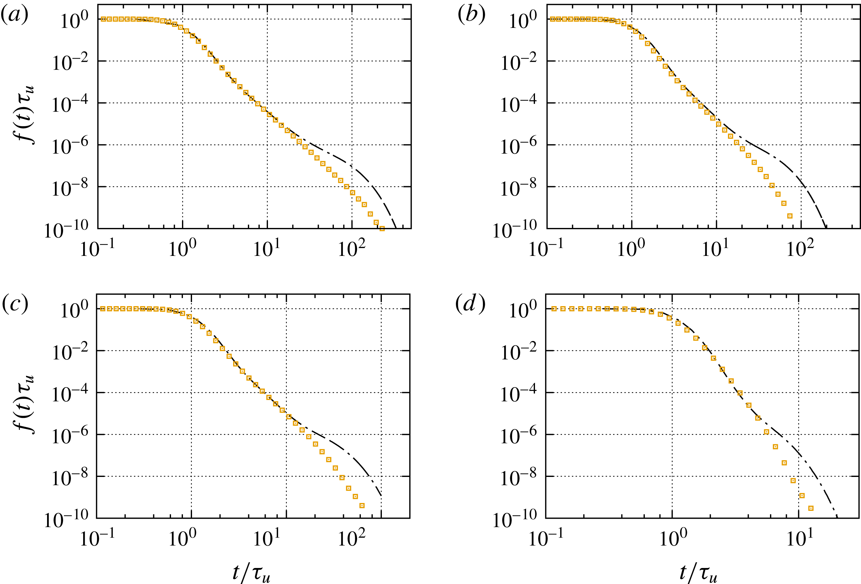
. The dash-dotted lines indicate the numerical data and the symbols the TDRW model for
 $\ell \approx \ell _{p}$
for
 $Pe=10^{3}$
,
 $\ell =0.77\ell _{p}$
for
 $Pe=5\times 10^{2}$
and
 $Pe=3\times 10^{2}$
, and
 $\ell =0.7\ell _{p}$
for
 $Pe=30$
.

We solve this TDRW model for the breakthrough curves using random walk particle tracking simulations. Figure 9 shows the results of this TDRW characterised by (4.18) compared with the direct numerical simulations of the pore-scale flow and transport problem. It should be noted that the TDRW is parameterised by the PDF of mean pore velocities and the Péclet number. For computational convenience, here and in the following, we approximate the PDF (3.14) of mean pore velocities by (3.16). The TDRW model captures the intermediate tailing of the breakthrough curves at all Péclet numbers correctly, which thus can be attributed to both heterogeneity in the mean pore velocity and diffusion.
It should be noted that the PDF of transition times (4.19) is not heavy tailed. The maximum transition time is given by
 $\ell ^{2}/2D$
, which determines the cutoff of (4.19). For smaller times, it behaves as
 $\unicode[STIX]{x1D713}_{m}(t)\propto t^{-3-\unicode[STIX]{x1D6FC}/2}$
, which can be seen by inserting (3.14) into (4.19) and rescaling of the integration variable. Thus, according to the central limit theorem, breakthrough curves at large distances from the inlet are expected to converge to a Fickian limit. In this sense, the tailing behaviour in the intermediate regime is preasymptotic and can be attributed to the distance from the inlet or sample size. At times longer than the characteristic diffusion time over the pore, the TDRW breakthrough curves are cut off and do not capture the second tailing regime characterised by first a flattening and then exponential cutoff. In the following, we discuss the origin of the second tailing regime in the light of trapping due to particle transitions across streamlines into low-velocity pores.
4.2 Solute trapping and release
In the previous section, we have focused on particle motion in the direction of the streamlines by the mean pore velocity, as illustrated schematically by the horizontal arrow in figure 7. Alternatively, particles may make diffusive transitions across streamlines into the wake of a solid grain, indicated by the vertical arrow in figure 7. In these regions, the flow velocity is close to zero and diffusion is the dominant transport mechanism. Thus, we denote these regions in the following as immobile zones.
We first focus solely on the impact of cross-diffusion into low-velocity zones and represent heterogeneity of the pore velocities in terms of the average velocity
 $\langle v_{e}\rangle$
and the hydrodynamic dispersion coefficients
 ${\mathcal{D}}$
determined above. This means that we assume that advective heterogeneity can be homogenised by advection–dispersion. Below, in § 4.3, we combine the effects of heterogeneous advection and diffusion into immobile zones. As we assume that mobile transport is homogenised, there is no characteristic transition length scale, in contrast to the previous sections, where the pore length
 $\ell$
marks the correlation scale of the streamwise velocities. Velocity fluctuations are quantified by hydrodynamic dispersion. Thus, in terms of the advective–diffusive TDRW introduced in the previous section, this means that particles perform spatial transitions over a distance
 $\unicode[STIX]{x0394}s\ll L$
, which now merely represents a discretisation of space (Russian et al.
Reference Russian, Dentz and Gouze2016). Particle transitions in space then are characterised by (4.16) and (4.17) with the substitutions
 $$\begin{eqnarray}\displaystyle & \displaystyle \ell \rightarrow \unicode[STIX]{x0394}s,\quad v\rightarrow \langle v_{e}\rangle ,\quad D\rightarrow {\mathcal{D}}. & \displaystyle\end{eqnarray}$$
Particle transitions in time now are composed of a mobile time
 $\unicode[STIX]{x1D70F}_{0}$
, which represents advective–dispersive motion in the mean flow direction and the time of trapping in immobile zones as
 $\unicode[STIX]{x1D70F}=\unicode[STIX]{x1D70F}_{0}+\unicode[STIX]{x1D70F}_{im}(\unicode[STIX]{x1D70F}_{0})$
. The mobile time is distributed according to (4.15) with the substitutions (4.21). The immobile time
 $\unicode[STIX]{x1D70F}_{im}$
is determined based on the assumption that immobile zones are uniformly distributed in the medium. As the characteristic time scale between trapping events is given by the characteristic cross-diffusion time, trapping events can be assumed to occur at a constant rate
 $\unicode[STIX]{x1D6FE}$
. This means that the number of trapping events
 $n_{\unicode[STIX]{x1D70F}_{0}}$
that occur during a time
 $\unicode[STIX]{x1D70F}_{0}$
is Poisson distributed,
 $$\begin{eqnarray}\displaystyle & \displaystyle p_{n}(n|\unicode[STIX]{x1D70F}_{0})=\frac{(\unicode[STIX]{x1D6FE}\unicode[STIX]{x1D70F}_{0})^{n}\exp (-\unicode[STIX]{x1D6FE}\unicode[STIX]{x1D70F}_{0})}{n!}. & \displaystyle\end{eqnarray}$$
Thus, the immobile time
 $\unicode[STIX]{x1D70F}_{im}$
during a mobile transition of duration
 $\unicode[STIX]{x1D70F}_{0}$
is given by the sum over the
 $n_{\unicode[STIX]{x1D70F}_{0}}$
individual trapping times times
 $\unicode[STIX]{x1D70F}_{f}$
,
 $$\begin{eqnarray}\displaystyle & \displaystyle \unicode[STIX]{x1D70F}_{im}(\unicode[STIX]{x1D70F}_{0})=\mathop{\sum }_{k=1}^{n_{\unicode[STIX]{x1D70F}_{0}}}\unicode[STIX]{x1D70F}_{f,k}. & \displaystyle\end{eqnarray}$$
It is a compound Poisson process (Feller Reference Feller1968). The trapping times
 $\unicode[STIX]{x1D70F}_{f}$
are independent identically distributed according to
 $p_{f}(t)$
, which is determined below. The compound Poisson process (4.23) is characterised by the PDF
 $\unicode[STIX]{x1D713}_{f}(t|\unicode[STIX]{x1D70F}_{0})$
, whose Laplace transform is given by (Margolin, Dentz & Berkowitz Reference Margolin, Dentz and Berkowitz2003)
 $$\begin{eqnarray}\displaystyle & \displaystyle \unicode[STIX]{x1D713}_{f}^{\ast }(\unicode[STIX]{x1D706}|\unicode[STIX]{x1D70F}_{0})=\exp (-\{\unicode[STIX]{x1D6FE}[1-p_{f}^{\ast }(\unicode[STIX]{x1D706})]\}\unicode[STIX]{x1D70F}_{0}). & \displaystyle\end{eqnarray}$$
In order to quantify the impact of cross-diffusion on macroscale transport, we need to determine the distribution of trapping times
 $\unicode[STIX]{x1D70F}_{f}$
and the trapping rate
 $\unicode[STIX]{x1D6FE}$
. To this end, we first note that the total concentration can be decomposed into the concentration of the solute
 $c_{m}(x,t)$
in the mobile and
 $c_{im}(x,t)$
in the immobile regions,
 $\overline{c}(x,t)=c_{m}(x,t)+c_{im}(x,t)$
. It should be noted that here both mobile and immobile concentrations refer to the same support volume. The mobile concentration in this TDRW framework is described by the non-local advection–diffusion equation (Margolin et al.
Reference Margolin, Dentz and Berkowitz2003; Benson & Meerschaert Reference Benson and Meerschaert2009; Comolli et al.
Reference Comolli, Hidalgo, Moussey and Dentz2016; Russian et al.
Reference Russian, Dentz and Gouze2016)
 $$\begin{eqnarray}\displaystyle & \displaystyle \frac{\unicode[STIX]{x2202}c_{m}(x,t)}{\unicode[STIX]{x2202}t}+\langle u_{1}\rangle \frac{\unicode[STIX]{x2202}c_{m}(x,t)}{\unicode[STIX]{x2202}x}-{\mathcal{D}}\frac{\unicode[STIX]{x2202}^{2}c_{m}(x,t)}{\unicode[STIX]{x2202}x^{2}}=-\frac{\unicode[STIX]{x2202}c_{im}(x,t)}{\unicode[STIX]{x2202}t}. & \displaystyle\end{eqnarray}$$
The immobile concentration
 $c_{im}(x,t)$
is given by
 $$\begin{eqnarray}\displaystyle & \displaystyle c_{im}(x,t)=\int _{0}^{t}\,\text{d}t^{\prime }\left[\int _{t-t^{\prime }}^{\infty }\,\text{d}t^{\prime \prime }p_{f}(t^{\prime \prime })\right]\unicode[STIX]{x1D6FE}c_{m}(x,t^{\prime }). & \displaystyle\end{eqnarray}$$
The expression in the square brackets denotes the probability that the trapping time is larger than
 $t-t^{\prime }$
. This means that the immobile concentration is given by the probability per time that a particle enters the immobile zone, expressed by
 $\unicode[STIX]{x1D6FE}c_{m}(x,t)$
, times the probability that it stays there for a time larger than the observation time. The ratio
 $\unicode[STIX]{x1D6FD}$
of total mass in the immobile and mobile zones at equilibrium is obtained from (4.26) as
 $$\begin{eqnarray}\displaystyle & \displaystyle \unicode[STIX]{x1D6FD}=\unicode[STIX]{x1D6FE}\langle \unicode[STIX]{x1D70F}_{f}\rangle . & \displaystyle\end{eqnarray}$$
It should be noted that (4.25) describes solute transport in the multirate mass transfer approach (Haggerty & Gorelick Reference Haggerty and Gorelick1995; Carrera et al.
Reference Carrera, Sánchez-Vila, Benet, Medina, Galarza and Guimerà1998; Comolli et al.
Reference Comolli, Hidalgo, Moussey and Dentz2016). In this framework,
 $\unicode[STIX]{x1D6FD}$
is equal to the ratio between the immobile
 $\unicode[STIX]{x1D719}_{im}$
and mobile
 $\unicode[STIX]{x1D719}_{m}$
volume fractions. Thus, the trapping rate is given by
 $$\begin{eqnarray}\displaystyle & \displaystyle \unicode[STIX]{x1D6FE}=\frac{\unicode[STIX]{x1D719}_{im}}{\unicode[STIX]{x1D719}_{m}\langle \unicode[STIX]{x1D70F}_{f}\rangle }. & \displaystyle\end{eqnarray}$$
Using the mobile and immobile volume fractions, the total concentration
 $\overline{c}(x,t)$
can be written in terms of
 $g_{m}(x,t)=c_{m}(x,t)/\unicode[STIX]{x1D719}_{m}$
and
 $g_{im}(x,t)=c_{im}(x,t)/\unicode[STIX]{x1D719}_{im}$
, which refer to the mobile and immobile subvolumes, as
 $\overline{c}(x,t)=\unicode[STIX]{x1D719}_{m}g_{m}(x,t)+\unicode[STIX]{x1D719}_{im}g_{im}(x,t)$
.
Breakthrough curves for
 $Pe=10^{3}$
,
 $3\times 10^{2}$
,
 $30$
and
 $3$
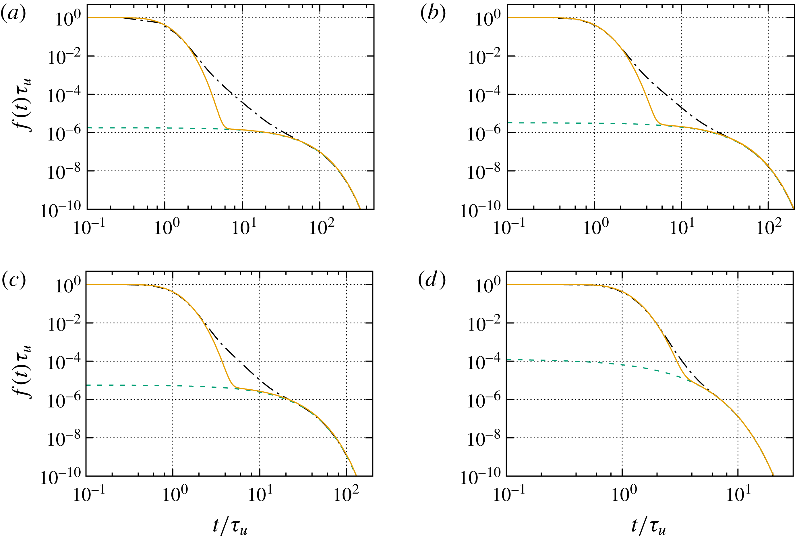
. The dash-dotted lines indicate the numerical data and the circles indicate the exponential estimation of the tailing behaviour, from which we obtain the values for
 $\langle \unicode[STIX]{x1D70F}_{f}\rangle$
and
 $\unicode[STIX]{x1D6FE}$
displayed in figure 11 below.

From (4.25), we obtain for the long-time behaviour of the breakthrough curves the following behaviour:
 $$\begin{eqnarray}\displaystyle & \displaystyle f(t)=\unicode[STIX]{x1D70F}_{u}\unicode[STIX]{x1D6FE}\int _{t}^{\infty }\,\text{d}t^{\prime }p_{f}(t), & \displaystyle\end{eqnarray}$$
for
 $t\gg \unicode[STIX]{x1D70F}_{u}$
. The full solution for
 $f(t)$
and the derivation of this approximation are detailed in appendix D. This means that the tailing behaviour is fully determined in terms of the PDF of trapping times. Figure 10 shows that the tail of the breakthrough curve can well approximated by an exponential function, which implies that the distribution of trapping times can be represented by an exponential PDF. In fact, the distribution of diffusion times in an immobile zone of size
 $\ell$
can be obtained through the solution of a diffusion problem, as outlined in appendix D. The average trapping time is related to the characteristic diffusion time
 $\unicode[STIX]{x1D70F}_{D}=\ell ^{2}/(2D)$
in a domain of length
 $\ell$
. The PDF of trapping times for such a problem is well approximated again by the exponential distribution as (Delay, Porel & Sardini Reference Delay, Porel and Sardini2002; Dentz et al.
Reference Dentz, Gouze, Russian, Dweik and Delay2012).
 $$\begin{eqnarray}\displaystyle & \displaystyle p_{f}(t)=\frac{\exp (-t/\langle \unicode[STIX]{x1D70F}_{f}\rangle )}{\langle \unicode[STIX]{x1D70F}_{f}\rangle }; & \displaystyle\end{eqnarray}$$
see also appendix E. The mean trapping time is
 $\langle \unicode[STIX]{x1D70F}_{f}\rangle =r\unicode[STIX]{x1D70F}_{D}$
, with
 $r\sim 1$
. The tail of the breakthrough curve is thus given by
 $$\begin{eqnarray}\displaystyle & \displaystyle f(t)=\unicode[STIX]{x1D70F}_{u}\unicode[STIX]{x1D6FE}\exp (-t/r\unicode[STIX]{x1D70F}_{D}). & \displaystyle\end{eqnarray}$$
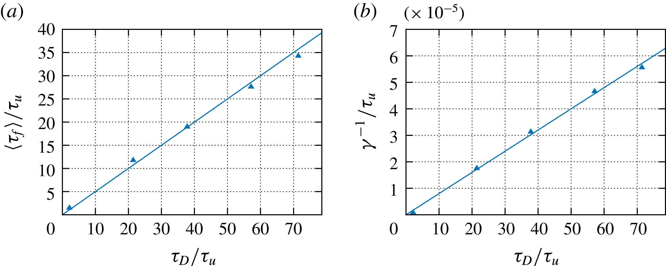
This means that we can obtain both the trapping rate and the mean trapping time from the tails of the breakthrough curves at different Péclet numbers. According to our reasoning, both depend on
 $\unicode[STIX]{x1D70F}_{D}$
as
 $$\begin{eqnarray}\displaystyle & \displaystyle \langle \unicode[STIX]{x1D70F}_{f}\rangle =r\unicode[STIX]{x1D70F}_{D},\quad \unicode[STIX]{x1D6FE}=\frac{\unicode[STIX]{x1D6FD}}{r\unicode[STIX]{x1D70F}_{D}}. & \displaystyle\end{eqnarray}$$
The dependences of
 $\langle \unicode[STIX]{x1D70F}_{f}\rangle$
and
 $\unicode[STIX]{x1D6FE}^{-1}$
on
 $\unicode[STIX]{x1D70F}_{D}$
estimated from the numerical data are shown in figure 11. From the data, we obtain
 $r\approx 1/2$
and
 $\unicode[STIX]{x1D6FD}\approx 2.5\times 10^{-4}$
, which is consistent with the probability of obtaining velocities smaller than
 $10^{-3}\langle v\rangle$
, which we deem immobile. It should be noted from figure 4 that the PDF of the velocity magnitude deviates from the flat behaviour characteristic for in-pore velocities at
 $10^{-3}$
and increases towards lower velocities. This increase may be assigned to low velocities in immobile zones.
(a) Mean trapping time
 $\langle \unicode[STIX]{x1D70F}_{f}\rangle$
versus
 $\unicode[STIX]{x1D70F}_{D}$
estimated from the data and (solid line) linear estimation with
 $r=1/2$
. (b) Inverse trapping rate versus
 $\unicode[STIX]{x1D70F}_{D}$
and linear estimate with
 $\unicode[STIX]{x1D6FD}=2.5\times 10^{-4}$
.

Figure 10 compares the breakthrough curves obtained from the solution of (4.25) (see appendix D) parameterised with an exponential PDF of trapping times and the average trapping times and trapping rates given by (4.32) as well as the mean velocity
 $\langle u_{1}\rangle$
and hydrodynamic dispersion coefficient
 ${\mathcal{D}}$
. It captures well the onset of decay of the breakthrough curves, just like the ADE solution discussed above, and the exponential long-time tail. The onset of the exponential tail depends on the trapping rate
 $\unicode[STIX]{x1D6FE}$
and the exponential cutoff time is given by the diffusion time scale
 $\unicode[STIX]{x1D70F}_{D}$
. As expected, this TDRW model does not represent the intermediate tailing due to heterogeneous pore velocities. The quantification of the combined effect of trapping and heterogeneous advection is discussed in the next section.
4.3 Advective heterogeneity and trapping
In this section, we integrate heterogeneous pore-scale advection and diffusion into immobile zones into a TDRW approach that quantifies the dominant pore-scale transport mechanisms. This approach models mobile particle transition over the length of a pore, as detailed in § 4.1.2. Solute trapping is modelled as discussed in the previous section. Specifically, the number of trapping events is given by the Poisson distribution (4.22) conditioned on the time
 $\unicode[STIX]{x1D70F}_{m}=\ell /v$
for a mobile transition. Thus, the transition time in this integrated TDRW is (Comolli et al.
Reference Comolli, Hidalgo, Moussey and Dentz2016; Russian et al.
Reference Russian, Dentz and Gouze2016)
 $$\begin{eqnarray}\displaystyle & \displaystyle \unicode[STIX]{x1D70F}=\unicode[STIX]{x1D70F}_{m}+\mathop{\sum }_{k=1}^{n_{\unicode[STIX]{x1D70F}_{m}}}\unicode[STIX]{x1D70F}_{f,k}, & \displaystyle\end{eqnarray}$$
where
 $n_{\unicode[STIX]{x1D70F}_{m}}$
is distributed according to the Poisson distribution
 $p_{n}(n|\unicode[STIX]{x1D70F}_{m})$
and
 $\unicode[STIX]{x1D70F}_{f}$
according to (4.30). It should be noted that the total trapping time during a mobile transition given by the second term on the right-hand side of (4.33) is a compound Poisson process. The joint PDF
 $\unicode[STIX]{x1D713}(x,t)$
of transition lengths
 $\unicode[STIX]{x1D709}$
and time
 $\unicode[STIX]{x1D70F}$
can then be expressed in Laplace space in terms of the Laplace transforms of
 $\unicode[STIX]{x1D713}_{m}(t)$
, the PDF of mobile times and the trapping time PDF
 $p_{f}(t)$
as
 $$\begin{eqnarray}\displaystyle & \displaystyle \unicode[STIX]{x1D713}^{\ast }(x,\unicode[STIX]{x1D706})=\unicode[STIX]{x1D713}_{m}^{\ast }(x,\unicode[STIX]{x1D706}+\unicode[STIX]{x1D6FE}[1-p_{f}^{\ast }(\unicode[STIX]{x1D706})]); & \displaystyle\end{eqnarray}$$
see appendix C. The distribution of transition times is given accordingly by
 $$\begin{eqnarray}\displaystyle & \displaystyle \unicode[STIX]{x1D713}^{\ast }(\unicode[STIX]{x1D706})=\unicode[STIX]{x1D713}_{m}^{\ast }(\unicode[STIX]{x1D706}+\unicode[STIX]{x1D6FE}[1-p_{f}^{\ast }(\unicode[STIX]{x1D706})]). & \displaystyle\end{eqnarray}$$
With these results, we obtain for the velocity and diffusion kernels (4.6a ) and (4.6b ) the Laplace space expressions
 $$\begin{eqnarray}\displaystyle & \displaystyle \unicode[STIX]{x1D708}^{\ast }(\unicode[STIX]{x1D706})=\frac{\unicode[STIX]{x1D708}_{m}[\unicode[STIX]{x1D706}\unicode[STIX]{x1D6F7}^{\ast }(\unicode[STIX]{x1D706})]}{\unicode[STIX]{x1D6F7}^{\ast }(\unicode[STIX]{x1D706})}, & \displaystyle\end{eqnarray}$$
 $$\begin{eqnarray}\displaystyle & \displaystyle \unicode[STIX]{x1D705}^{\ast }(\unicode[STIX]{x1D706})=\frac{\unicode[STIX]{x1D705}_{m}[\unicode[STIX]{x1D706}\unicode[STIX]{x1D6F7}^{\ast }(\unicode[STIX]{x1D706})]}{\unicode[STIX]{x1D6F7}^{\ast }(\unicode[STIX]{x1D706})}, & \displaystyle\end{eqnarray}$$
 $\unicode[STIX]{x1D6F7}^{\ast }(\unicode[STIX]{x1D706})=1+\unicode[STIX]{x1D706}^{-1}\unicode[STIX]{x1D6FE}[1-p_{f}^{\ast }(\unicode[STIX]{x1D706})]$
; see appendix B. Following the developments in the previous section, we define the immobile concentration
 $c_{im}(x,t)$
in terms of the mobile concentration as in (4.26). Thus, based on this relation and expressions (4.36) for the kernels, we derive from (4.5) the following governing equation for the solute concentration in the mobile regions:
 $$\begin{eqnarray}\displaystyle & & \displaystyle \frac{\unicode[STIX]{x2202}c_{m}(x,t)}{\unicode[STIX]{x2202}t}+\frac{\unicode[STIX]{x2202}}{\unicode[STIX]{x2202}t}\int _{0}^{t}\,\text{d}t^{\prime }\left[\int _{t-t^{\prime }}^{\infty }\,\text{d}t^{\prime \prime }p_{f}(t^{\prime \prime })\right]\unicode[STIX]{x1D6FE}c_{m}(x,t^{\prime })=\nonumber\\ \displaystyle & & \displaystyle \quad -\,\int _{0}^{t}\,\text{d}t^{\prime }\int _{0}^{t-t^{\prime }}\,\text{d}t^{\prime \prime }\left[\unicode[STIX]{x1D708}_{m}(t^{\prime \prime })\frac{\unicode[STIX]{x2202}}{\unicode[STIX]{x2202}x}-\unicode[STIX]{x1D705}_{m}(t^{\prime \prime })\frac{\unicode[STIX]{x2202}^{2}}{\unicode[STIX]{x2202}x^{2}}\right]\unicode[STIX]{x1D713}_{f}(t-t^{\prime }-t^{\prime \prime }|t^{\prime \prime })c_{m}(x,t^{\prime });\end{eqnarray}$$
see appendix F. The second term on the left-hand side denotes the change of the mobile solute concentration due to mass transfer with the immobile regions. The term on the right-hand side denotes the solute flux in the mobile region during the period of time
 $t^{\prime \prime }$
for which particles are making mobile transitions. It should be noted that
 $\unicode[STIX]{x1D713}_{f}(t-t^{\prime }-t^{\prime \prime }|t^{\prime \prime })$
denotes the probability that the particle is trapped during the time
 $t-t^{\prime }-t^{\prime \prime }$
for a given mobile duration
 $t^{\prime \prime }$
.
Breakthrough curves for
 $Pe=10^{3}$
,
 $5\times 10^{2}$
,
 $3\times 10^{2}$
and
 $30$
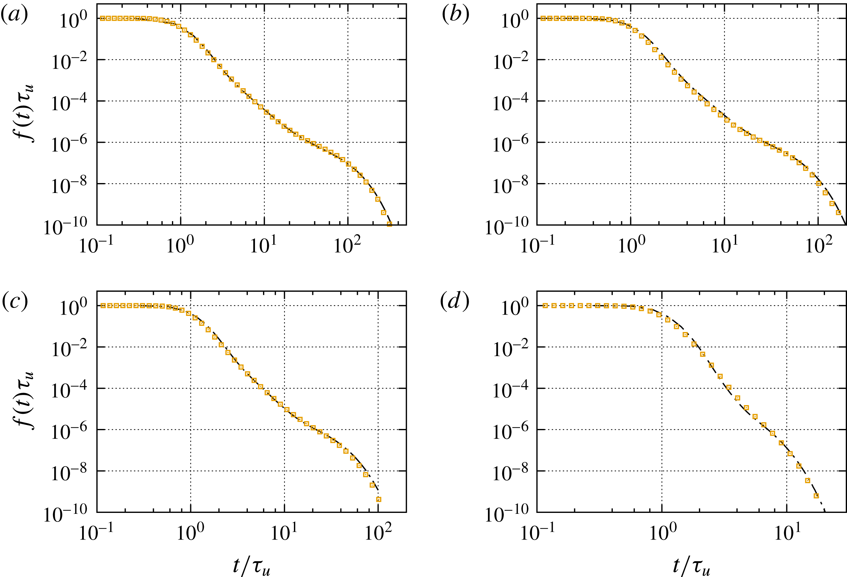
. The dash-dotted lines indicate the numerical results. The symbols denote the result of the TDRW model including heterogeneous advection and trapping in immobile zones. The TDRW model uses the parameter values given in the captions of figures 9 and 10.

We solve this TDRW model for macroscale transport using random walk particle tracking simulations. The transport behaviour is parameterised in terms of the PDF of mean pore velocities, the trapping rate
 $\unicode[STIX]{x1D6FE}$
, (4.28), and the distribution (4.30) of trapping times discussed in the previous section. Thus, in principle, macroscale transport can be understood in terms of the medium geometry (distribution of pore diameters), hydrodynamics (Poiseuille’s law) and diffusion along and across streamlines into immobile regions.
Figure 12 compares the breakthrough curves from the direct numerical simulations with the behaviour of the TDRW approach. The TDRW model and simulation data compare well for all Péclet numbers. The intermediate tailing is well captured by the distribution of mean pore velocities and diffusion in the mean flow direction, as discussed in § 4.1.2. The exponential tail is picked up by the mass transfer model discussed in the previous section. Moreover, the transitions from the intermediate advective tailing behaviour to the exponential are well represented for all Péclet numbers. The proposed model captures all aspects of the observed solute breakthrough curves based on the identification and quantification of the dominant pore-scale transport mechanisms.
5 Summary and conclusions
We have studied and quantified the advection and diffusion mechanisms of preasymptotic pore-scale transport and their relations to the statistical medium and flow properties in terms of the pore-size distribution and the distribution of the magnitude of the Eulerian velocity. Our study uses data from high-performance computational fluid dynamics simulations of flow and solute transport in a synthetic three-dimensional porous medium. The medium properties resemble the characteristics of sand or bead packs in grain size distribution and porosity.
We focus on the complementary solute breakthrough curves at the outlet of the porous medium, to which we refer as breakthrough curves for simplicity. The advection–dispersion paradigm predicts an exponential decrease of the breakthrough curve from
 $1$
towards
 $0$
at the mean advection time over the domain length with a width given in terms of the longitudinal hydrodynamic dispersion coefficient. For all
 $Pe\gg 1$
, we observe pronounced deviations from this behaviour, which increase with increasing
 $Pe$
. The breakthrough curves display two non-Fickian regimes. The intermediate regime is given by a sub-exponential decay, which can be attributed to advective heterogeneity. The second regime is characterised by a flattening of the sub-exponential behaviour before it is cut off exponentially rapidly. This behaviour can be attributed to diffusion across streamlines into the immobile regions in the wake of solid grains.
In order to quantify these behaviours in a macroscale transport model, we first develop a model for the statistics of the Eulerian velocity magnitude in terms of the pore-size distribution. This model relies on the assumption that the velocity profile in a single pore is parabolic and that its maximum velocity is related to the cross-sectional pore area through Poiseuille’s law. Thus, we obtain an estimate for the distribution of point-wise velocity magnitudes as well as an estimate for the distribution of mean pore velocities. The distribution of velocity magnitudes is characterised by a flat part at small velocities, which can be attributed to the flat distribution characteristic for velocities in single pores, and an exponential decay, which can be attributed to the pore-size distribution. The distribution of mean pore velocities is much narrower than the distribution of the Eulerian velocity magnitude, with smooth cutoffs at low and high velocity magnitudes.
Then, we cast the advective–diffusive pore-scale particle motion in terms of a time-domain random walk (TDRW), based on the fact that flow velocities vary little over the characteristic pore length. We first consider purely advective particle transitions such that the distribution of residence times is given in terms of the distribution of the Eulerian velocity magnitude. It scales as
 $t^{-3}$
, which implies a Levy-stable behaviour for the particle travel time distributions, and predicts a
 $Pe$
-independent persistent
 $t^{-2}$
scaling of the breakthrough curves. This approach ignores the impact of diffusion on pore-scale particle transport completely. Thus, in a next step, we account for the diffusive sampling of flow velocities in single pores. Based on the assumption that pores are on average much longer than wide, we approximate the effective particle velocity over a pore by the average pore velocity. This assumes that particles can sample the full pore velocity contrast during a transition. Thus, the distribution of effective particle velocities is set equal to the distribution of mean pore velocities. We also account for the diffusive cutoff of the residence time distribution in the case of diffusion-dominated transitions. The resulting TDRW captures the intermediate tailing of the breakthrough curves and the dependence on the Péclet number despite these drastic simplifications. The flattening of the breakthrough curve and asymptotic exponential cutoff is not accounted for. As mentioned above, this feature can be attributed to purely diffusive particle transitions across streamlines into the void space in the wake of solid grains that connect adjacent pores. This mechanism represents a trapping process, whose residence times can be characterised by an exponential distribution that decays on the diffusion time over a pore. The trapping rate can be related to the volume fractions of mobile and immobile pore regions and the inverse diffusion time. Trapping of particles is quantified in the TDRW framework by a compound Poisson process conditioned on the advective residence time. This approach captures the full behaviour of the breakthrough curves for all values of
 $Pe$
. The evolution of the particle density, or equivalently solute distribution, is governed by an integro-partial-differential equation, whose memory kernels are related to the distribution of mean pore velocities and the distribution of residence times in immobile pores. It should be noted that we have focused on global transport in the direction of the mean flow. The presented approach can be generalised to account for transverse mass transfer by determining the stochastic rules of transverse particle motion, which here is quantified in an average sense through tortuosity.
In conclusion, we have identified and quantified the dominant pore-scale advection and diffusion mechanism in a macroscale transport model that captures preasymptotic non-Fickian transport. This approach accounts for the impact of pore-scale heterogeneity on transport on the REV scale, which is manifested in tailing of the breakthrough curves as an expression of pore-scale concentration heterogeneity. Thus, while the concept of the REV is valid for the definition of macroscale material properties such as porosity or permeability, it does not imply that transport is in local physical equilibrium. The occurrence of advective breakthrough curve tailing in the intermediate regime depends on the distance from the inlet and the distribution of characteristic advection time scales, while the non-Fickian asymptotic tail due to trapping in immobile zones depends on the characteristic diffusion time in the immobile regions. We suggest that the identified transport mechanisms are of a general nature beyond the sand-like model medium under consideration here. More complex porous media are characterised by broad distributions of pore diameters and immobile porosity (Gouze et al. Reference Gouze, Melean, Le Borgne, Dentz and Carrera2008; Bijeljic et al. Reference Bijeljic, Raeini, Mostaghimi and Blunt2013; Gjetvaj et al. Reference Gjetvaj, Russian, Gouze and Dentz2015), which emphasise the non-Fickian preasymptotic transport features and may delay the onset of an asymptotic hydrodynamic dispersion regime.
Acknowledgements
M.D. and J.J.H. gratefully acknowledge the support of the European Research Council (ERC) through the project MHetScale (617511) and the support of the Spanish Ministry of Economy, Industry and Competitivity through the project MECMAT (CGL2016-80022-R). M.I. gratefully acknowledges the financial support provided by AVL and the computing facilities provided by the Warwick Centre for Scientific Computing.
Appendix A. Numerical simulations
The standard OpenFOAM solvers simpleFoam and scalarTransportFoam were used to perform flow and transport simulations. The latter was modified to allow for runtime co-processing of volumetric and PDF information.
A blended forward Euler/Crank–Nicolson discretisation in time was used which ensured
 $\unicode[STIX]{x0394}t<\unicode[STIX]{x0394}x^{2}/D$
for accurate time resolution. A second-order upwind scheme was used for advection to minimise numerical dispersion, a second-order least-squares approach was used for computing gradients and a central scheme for diffusive fluxes.
The simulations were performed on an irregular grid to represent the grain boundaries well. Details on the mesh generation and numerical method are given in Icardi et al. (Reference Icardi, Boccardo, Marchisio, Tosco and Sethi2014). In Sections III and IV of this paper, the interested reader finds a detailed grid independence study of the flow and transport simulations. The number of mesh cells used for the numerical solution was
 $41\times 10^{6}$
. The largest cell size was
 $\ell _{c}=1/200$
and the smallest
 $\ell _{c}=1/1600$
of the domain size. Simulations were performed on 128 Intel Xeon E5-2630 2.4GHz cores and, due to the significant tailing, had to be run for long times, resulting in approximately 48 h of simulation time per each run.
Regarding the issue of numerical dispersion, for the numerical simulations used in the paper, the maximum grid Péclet number
 $Pe_{g}=\ell _{c}v/D$
varied between
 $Pe_{g}\approx 5$
for the
 $Pe=10^{3}$
case and
 $Pe_{g}\approx 0.15$
for the
 $Pe=30$
case. It should be noted that these are the maximum grid Péclet numbers, which are obtained in the pore centres, where the resolution is coarsest and velocities are relatively high, of the order of the mean velocity. As both the mesh size and the velocity vary, the grid Péclet numbers close to grains and in the wake of the grains, where the resolutions are high (i.e. small
 $\ell _{c}$
) and velocities are low, are
 $Pe_{g}\ll 1$
. Moreover, it should be noted that for the breakthrough curves under consideration (e.g. figure 3), the effect of hydrodynamic dispersion due to flow variability (in high flow velocities), which is of the order of
 $\overline{v}\ell _{0}$
, overshadows the possible effect of numerical dispersion in the pore centres, which would otherwise only be visible in the initial decay of the breakthrough curve. The tailings in the two intermediate regimes are caused by variability in low velocities (high velocities give rise to the hydrodynamic dispersion effect) and dominant diffusion in immobile zones, for which the local grid Péclet numbers are much smaller than 1. For this reason, we are confident that the numerical simulations accurately reflect the actual physical mass transfer processes in the porous medium.
Appendix B. Kernels
We derive here expressions (4.20) and (4.36). To this end, we consider the
 $i$
th moments of the Laplace transform of the
 $\unicode[STIX]{x1D713}(x,t)$
,
 $$\begin{eqnarray}\displaystyle & \displaystyle \unicode[STIX]{x1D707}_{i}^{\ast }(\unicode[STIX]{x1D706})=\int \,\text{d}xx^{i}\unicode[STIX]{x1D713}^{\ast }(x,\unicode[STIX]{x1D706}). & \displaystyle\end{eqnarray}$$
The Laplace transforms of the kernels (4.6) are then given in terms of the
 $\unicode[STIX]{x1D707}_{i}^{\ast }(\unicode[STIX]{x1D706})$
as
 $$\begin{eqnarray}\displaystyle & \displaystyle \unicode[STIX]{x1D708}^{\ast }(\unicode[STIX]{x1D706})=\frac{\unicode[STIX]{x1D707}_{1}^{\ast }(\unicode[STIX]{x1D706})}{1-\unicode[STIX]{x1D713}^{\ast }(\unicode[STIX]{x1D706})}, & \displaystyle\end{eqnarray}$$
 $$\begin{eqnarray}\displaystyle & \displaystyle \unicode[STIX]{x1D705}^{\ast }(\unicode[STIX]{x1D706})=\frac{1}{2}\frac{\unicode[STIX]{x1D707}_{2}^{\ast }(\unicode[STIX]{x1D706})}{1-\unicode[STIX]{x1D713}^{\ast }(\unicode[STIX]{x1D706})}. & \displaystyle\end{eqnarray}$$
We obtain by using the Laplace transform of (4.18)
 $$\begin{eqnarray}\displaystyle & \displaystyle \unicode[STIX]{x1D707}_{1,m}^{\ast }(\unicode[STIX]{x1D706})=\frac{\ell }{\unicode[STIX]{x1D712}}\int _{0}^{\infty }\,\text{d}v\frac{v^{2}\unicode[STIX]{x1D70F}_{v}p_{m}(v)}{\langle v_{e}\rangle }\frac{\unicode[STIX]{x1D706}\unicode[STIX]{x1D713}_{0}^{\ast }(\unicode[STIX]{x1D706}|v)}{1-\unicode[STIX]{x1D713}_{0}^{\ast }(\unicode[STIX]{x1D706}|v)}\left[1-\unicode[STIX]{x1D713}_{0}^{\ast }(\unicode[STIX]{x1D706}|v)\right], & \displaystyle\end{eqnarray}$$
 $$\begin{eqnarray}\displaystyle & \displaystyle \unicode[STIX]{x1D707}_{2,m}^{\ast }(\unicode[STIX]{x1D706})=\int _{0}^{\infty }\,\text{d}v\frac{2D+v\ell }{\unicode[STIX]{x1D712}^{2}}\frac{v\unicode[STIX]{x1D70F}_{v}p_{m}(v)}{\langle v_{e}\rangle }\frac{\unicode[STIX]{x1D706}\unicode[STIX]{x1D713}_{0}^{\ast }(\unicode[STIX]{x1D706}|v)}{1-\unicode[STIX]{x1D713}_{0}^{\ast }(\unicode[STIX]{x1D706}|v)}\left[1-\unicode[STIX]{x1D713}_{0}^{\ast }(\unicode[STIX]{x1D706}|v)\right]. & \displaystyle\end{eqnarray}$$
Insertion of the Laplace transform of the exponential
 $\unicode[STIX]{x1D713}_{0}(t|v)$
then gives
 $$\begin{eqnarray}\displaystyle & \displaystyle \unicode[STIX]{x1D707}_{1,m}^{\ast }(\unicode[STIX]{x1D706})=\frac{\ell }{\unicode[STIX]{x1D712}}\int _{0}^{\infty }\,\text{d}v\frac{v^{2}p_{m}(v)}{\langle v_{e}\rangle }\left[1-\unicode[STIX]{x1D713}_{0}^{\ast }(\unicode[STIX]{x1D706}|v)\right], & \displaystyle\end{eqnarray}$$
 $$\begin{eqnarray}\displaystyle & \displaystyle \unicode[STIX]{x1D707}_{2,m}^{\ast }(\unicode[STIX]{x1D706})=\int _{0}^{\infty }\,\text{d}v\frac{2D+v\ell }{\unicode[STIX]{x1D712}^{2}}\frac{vp_{m}(v)}{\langle v_{e}\rangle }\left[1-\unicode[STIX]{x1D713}_{0}^{\ast }(\unicode[STIX]{x1D706}|v)\right]. & \displaystyle\end{eqnarray}$$
Insertion of these expressions into (B2) gives (4.20).
Similarly, we obtain by using (4.34) in (B2)
 $$\begin{eqnarray}\displaystyle & \displaystyle \unicode[STIX]{x1D707}_{1}^{\ast }(\unicode[STIX]{x1D706})=\frac{\ell }{\unicode[STIX]{x1D712}}\int _{0}^{\infty }\,\text{d}v\frac{v^{2}\unicode[STIX]{x1D70F}_{v}p_{m}(v)}{\langle v_{e}\rangle }\frac{\unicode[STIX]{x1D706}\unicode[STIX]{x1D6F7}^{\ast }(\unicode[STIX]{x1D706})\unicode[STIX]{x1D713}_{0}^{\ast }[\unicode[STIX]{x1D706}\unicode[STIX]{x1D6F7}^{\ast }(\unicode[STIX]{x1D706})|v]}{1-\unicode[STIX]{x1D713}_{0}^{\ast }[\unicode[STIX]{x1D706}\unicode[STIX]{x1D6F7}^{\ast }(\unicode[STIX]{x1D706})|v]}\frac{1-\unicode[STIX]{x1D713}_{0}^{\ast }[\unicode[STIX]{x1D706}\unicode[STIX]{x1D6F7}^{\ast }(\unicode[STIX]{x1D706})|v]}{\unicode[STIX]{x1D6F7}^{\ast }(\unicode[STIX]{x1D706})}, & \displaystyle\end{eqnarray}$$
 $$\begin{eqnarray}\displaystyle & \displaystyle \unicode[STIX]{x1D707}_{2}^{\ast }(\unicode[STIX]{x1D706})=\int _{0}^{\infty }\,\text{d}v\frac{2D+v\ell }{\unicode[STIX]{x1D712}^{2}}\frac{v\unicode[STIX]{x1D70F}_{v}p_{m}(v)}{\langle v_{e}\rangle }\frac{\unicode[STIX]{x1D706}\unicode[STIX]{x1D6F7}^{\ast }(\unicode[STIX]{x1D706})\unicode[STIX]{x1D713}_{0}^{\ast }[\unicode[STIX]{x1D706}\unicode[STIX]{x1D6F7}^{\ast }(\unicode[STIX]{x1D706})|v]}{1-\unicode[STIX]{x1D713}_{0}^{\ast }[\unicode[STIX]{x1D706}\unicode[STIX]{x1D6F7}^{\ast }(\unicode[STIX]{x1D706})|v]}\frac{1-\unicode[STIX]{x1D713}_{0}^{\ast }[\unicode[STIX]{x1D706}\unicode[STIX]{x1D6F7}^{\ast }(\unicode[STIX]{x1D706})|v]}{\unicode[STIX]{x1D6F7}^{\ast }(\unicode[STIX]{x1D706})}, & \displaystyle\end{eqnarray}$$
where we have defined
 $\unicode[STIX]{x1D6F7}^{\ast }(\unicode[STIX]{x1D706})=1+\unicode[STIX]{x1D706}^{-1}\unicode[STIX]{x1D6FE}[1-p_{f}^{\ast }(\unicode[STIX]{x1D706})]$
. Insertion of the Laplace transform of the exponential
 $\unicode[STIX]{x1D713}_{0}(t|v)$
then gives
 $$\begin{eqnarray}\displaystyle & \displaystyle \unicode[STIX]{x1D707}_{1}^{\ast }(\unicode[STIX]{x1D706})=\frac{\ell }{\unicode[STIX]{x1D712}}\int _{0}^{\infty }\,\text{d}v\frac{v^{2}p_{m}(v)}{\langle v_{e}\rangle }\frac{1-\unicode[STIX]{x1D713}_{0}^{\ast }[\unicode[STIX]{x1D706}\unicode[STIX]{x1D6F7}^{\ast }(\unicode[STIX]{x1D706})|v]}{\unicode[STIX]{x1D6F7}^{\ast }(\unicode[STIX]{x1D706})}, & \displaystyle\end{eqnarray}$$
 $$\begin{eqnarray}\displaystyle & \displaystyle \unicode[STIX]{x1D707}_{2}^{\ast }(\unicode[STIX]{x1D706})=\int _{0}^{\infty }\,\text{d}v\frac{2D+v\ell }{\unicode[STIX]{x1D712}^{2}}\frac{vp_{m}(v)}{\langle v_{e}\rangle }\frac{1-\unicode[STIX]{x1D713}_{0}^{\ast }[\unicode[STIX]{x1D706}\unicode[STIX]{x1D6F7}^{\ast }(\unicode[STIX]{x1D706})|v]}{\unicode[STIX]{x1D6F7}^{\ast }(\unicode[STIX]{x1D706})}. & \displaystyle\end{eqnarray}$$
By comparison with (B 5) and (B 6), we observe that
 $$\begin{eqnarray}\displaystyle & \displaystyle \unicode[STIX]{x1D707}_{1}^{\ast }(\unicode[STIX]{x1D706})=\frac{\unicode[STIX]{x1D707}_{1,m}^{\ast }[\unicode[STIX]{x1D706}\unicode[STIX]{x1D6F7}^{\ast }(\unicode[STIX]{x1D706})]}{\unicode[STIX]{x1D6F7}^{\ast }(\unicode[STIX]{x1D706})}, & \displaystyle\end{eqnarray}$$
 $$\begin{eqnarray}\displaystyle & \displaystyle \unicode[STIX]{x1D707}_{2}^{\ast }(\unicode[STIX]{x1D706})=\frac{\unicode[STIX]{x1D707}_{2,m}^{\ast }[\unicode[STIX]{x1D706}\unicode[STIX]{x1D6F7}^{\ast }(\unicode[STIX]{x1D706})]}{\unicode[STIX]{x1D6F7}^{\ast }(\unicode[STIX]{x1D706})}. & \displaystyle\end{eqnarray}$$
Appendix C. Transition time distribution
Here, we derive (4.34) for the Laplace transform of the transition time PDF for the case of heterogeneous advection and trapping. The trapping time, the second term in (4.33), is a compound Poisson process, whose distribution is
 $\unicode[STIX]{x1D713}_{f}(t|\unicode[STIX]{x1D70F}_{m})$
; see (4.24). Thus, for a given
 $\unicode[STIX]{x1D70F}_{m}$
, the Laplace transform of the PDF of the total transition time
 $\unicode[STIX]{x1D70F}_{m}+\unicode[STIX]{x1D70F}_{im}(\unicode[STIX]{x1D70F}_{m})$
is
 $$\begin{eqnarray}\displaystyle & \displaystyle \unicode[STIX]{x1D713}^{\ast }(\unicode[STIX]{x1D706}|\unicode[STIX]{x1D70F}_{m})=\exp (-\{\unicode[STIX]{x1D6FE}[1-p_{f}^{\ast }(\unicode[STIX]{x1D706})]\}\unicode[STIX]{x1D70F}_{m}-\unicode[STIX]{x1D706}\unicode[STIX]{x1D70F}_{m}). & \displaystyle\end{eqnarray}$$
For a given
 $v$
, the distribution of transition times is then obtained by averaging of (C 1) over the conditional distribution
 $\unicode[STIX]{x1D713}_{0}(t|v)$
of
 $\unicode[STIX]{x1D70F}_{m}$
 $$\begin{eqnarray}\displaystyle \displaystyle \unicode[STIX]{x1D713}^{\ast }(\unicode[STIX]{x1D706}|v) & = & \displaystyle \int _{0}^{\infty }\,\text{d}t\exp (-\{\unicode[STIX]{x1D706}+\unicode[STIX]{x1D6FE}[1-p_{f}^{\ast }(\unicode[STIX]{x1D706})]\}t-\unicode[STIX]{x1D706}t)\unicode[STIX]{x1D713}_{0}(t|v)\nonumber\\ \displaystyle & = & \displaystyle \unicode[STIX]{x1D713}_{0}^{\ast }(\unicode[STIX]{x1D706}+\unicode[STIX]{x1D6FE}[1-p_{f}^{\ast }(\unicode[STIX]{x1D706})]).\end{eqnarray}$$
The joint PDF of transition length and time is thus
 $$\begin{eqnarray}\displaystyle & \displaystyle \unicode[STIX]{x1D713}^{\ast }(\unicode[STIX]{x1D706})=\int _{0}^{\infty }\,\text{d}v\frac{vp_{m}(v)}{\langle v_{e}\rangle }\unicode[STIX]{x1D713}_{0}^{\ast }(\unicode[STIX]{x1D706}+\unicode[STIX]{x1D6FE}[1-p_{f}^{\ast }(\unicode[STIX]{x1D706})])=\unicode[STIX]{x1D713}_{m}^{\ast }(\unicode[STIX]{x1D706}+\unicode[STIX]{x1D6FE}[1-p_{f}^{\ast }(\unicode[STIX]{x1D706})]). & \displaystyle\end{eqnarray}$$
Appendix D. Breakthrough curves
We determine here the solution for the breakthrough curve corresponding to the governing (4.25). As at the beginning of § 4 for the ADE model, we consider a semi-infinite domain, which is a good approximation for
 $Pe\gg 1$
, which is the case for all of the scenarios under consideration here. Furthermore, we notice that the Laplace transform of (4.25) is given by
 $$\begin{eqnarray}\displaystyle & \displaystyle \unicode[STIX]{x1D706}c_{m}^{\ast }(x,\unicode[STIX]{x1D706})+\langle u_{1}\rangle \frac{\unicode[STIX]{x2202}c_{m}^{\ast }(x,\unicode[STIX]{x1D706})}{\unicode[STIX]{x2202}x}-{\mathcal{D}}\frac{\unicode[STIX]{x2202}^{2}c_{m}^{\ast }(x,\unicode[STIX]{x1D706})}{\unicode[STIX]{x2202}x^{2}}=0, & \displaystyle\end{eqnarray}$$
where we have used (4.26) and the fact that the initial concentration is
 $0$
. Furthermore, we have defined
 $$\begin{eqnarray}\displaystyle & \displaystyle \unicode[STIX]{x1D711}^{\ast }(\unicode[STIX]{x1D706})=\unicode[STIX]{x1D706}^{-1}\left[1-p_{f}^{\ast }(\unicode[STIX]{x1D706})\right]. & \displaystyle\end{eqnarray}$$
It should be noted that (D 1) is identical in form to the Laplace transform of (2.6). Thus, the solution can be expressed in terms of the Laplace transform of (2.7) as (Dentz et al. Reference Dentz, Cortis, Scher and Berkowitz2004)
 $$\begin{eqnarray}\displaystyle & \displaystyle f^{\ast }(\unicode[STIX]{x1D706},x)=\frac{1}{\unicode[STIX]{x1D706}}-\frac{1}{\unicode[STIX]{x1D706}}\exp \left[-\frac{x\langle u_{1}\rangle }{2D}\left(\sqrt{1+4\frac{\unicode[STIX]{x1D706}D[1+\unicode[STIX]{x1D6FE}\unicode[STIX]{x1D711}^{\ast }(\unicode[STIX]{x1D706})]}{\langle u_{1}\rangle ^{2}}}\right)-1\right]. & \displaystyle\end{eqnarray}$$
The solutions of (4.25) for the breakthrough curves displayed in figure 10 are obtained by numerical inverse Laplace transform of (D 3). In the limit
 $\unicode[STIX]{x1D706}D/\langle u_{1}\rangle ^{2}\ll 1$
, we can expand the latter as
 $$\begin{eqnarray}\displaystyle & \displaystyle f^{\ast }(\unicode[STIX]{x1D706},x)=\frac{x[1+\unicode[STIX]{x1D6FE}\unicode[STIX]{x1D711}^{\ast }(\unicode[STIX]{x1D706})]}{\langle u_{1}\rangle }+\ldots , & \displaystyle\end{eqnarray}$$
where the dots denote subleading contributions. Thus, we obtain for
 $f(t,L)\equiv f(t)$
the long-time approximation (4.29).
Appendix E. Trapping time distribution
In order to make an estimate for the distribution of trapping times, we approximate diffusion into immobile pores as a one-dimensional first-passage problem. Particles are injected at
 $z=0$
and diffuse to the outlet at
 $z=\ell$
. The particle distribution
 $g(z,t)$
then follows the diffusion equation
 $$\begin{eqnarray}\displaystyle & \displaystyle \frac{\unicode[STIX]{x2202}g(z,t)}{\unicode[STIX]{x2202}t}-D\frac{\unicode[STIX]{x2202}^{2}g(z,t)}{\unicode[STIX]{x2202}z^{2}}=0 & \displaystyle\end{eqnarray}$$
for the boundary conditions
 $$\begin{eqnarray}\displaystyle & \displaystyle -D\frac{\unicode[STIX]{x2202}g(z=0,t)}{\unicode[STIX]{x2202}z}=\unicode[STIX]{x1D6FF}(t),\quad g(z=\ell ,t)=0 & \displaystyle\end{eqnarray}$$
and the initial condition
 $g(z,t=0)=0$
. The distribution of first-passage times at
 $z=\ell$
is given by the flux over the boundary as
 $$\begin{eqnarray}\displaystyle & \displaystyle p_{f}(t)=-D\frac{g(z=\ell ,t)}{\unicode[STIX]{x2202}z}. & \displaystyle\end{eqnarray}$$
The solution to (E 1) reads in Laplace space as
 $$\begin{eqnarray}\displaystyle & \displaystyle g^{\ast }(z,\unicode[STIX]{x1D706})=\frac{\sinh \left[\sqrt{\frac{\unicode[STIX]{x1D706}}{D}}(\ell -z)\right]}{\sqrt{\unicode[STIX]{x1D706}D}\cosh \left(\sqrt{2\unicode[STIX]{x1D706}\unicode[STIX]{x1D70F}_{D}}\right)}. & \displaystyle\end{eqnarray}$$
Use of the latter in the Laplace transform of (E 3) gives
 $$\begin{eqnarray}\displaystyle & \displaystyle p_{f}^{\ast }(\unicode[STIX]{x1D706})=\frac{1}{\cosh \left(\sqrt{2\unicode[STIX]{x1D706}\unicode[STIX]{x1D70F}_{D}}\right)}. & \displaystyle\end{eqnarray}$$
For
 $\unicode[STIX]{x1D706}\unicode[STIX]{x1D70F}_{D}\ll 1$
, (E 5) can be approximated by
 $$\begin{eqnarray}\displaystyle & \displaystyle p_{f}^{\ast }(\unicode[STIX]{x1D706})\approx \frac{1}{1+\unicode[STIX]{x1D706}\unicode[STIX]{x1D70F}_{D}}, & \displaystyle\end{eqnarray}$$
whose inverse Laplace transform is given by (4.30).
Appendix F. Governing equation under heterogeneous advection and trapping
In order to derive (4.37), we note that the governing equation for the Laplace transform
 $\overline{c}^{\ast }(x,\unicode[STIX]{x1D706})$
follows from (4.5) and (4.36) as
 $$\begin{eqnarray}\displaystyle & \displaystyle \unicode[STIX]{x1D706}\overline{c}^{\ast }(x,\unicode[STIX]{x1D706})+\left(\unicode[STIX]{x1D708}_{m}^{\ast }[\unicode[STIX]{x1D706}\unicode[STIX]{x1D6F7}^{\ast }(\unicode[STIX]{x1D706})]\frac{\unicode[STIX]{x2202}}{\unicode[STIX]{x2202}x}-\unicode[STIX]{x1D705}_{m}^{\ast }[\unicode[STIX]{x1D706}\unicode[STIX]{x1D6F7}^{\ast }(\unicode[STIX]{x1D706})]\frac{\unicode[STIX]{x2202}^{2}}{\unicode[STIX]{x2202}x^{2}}\right)\frac{\overline{c}^{\ast }(x,\unicode[STIX]{x1D706})}{\unicode[STIX]{x1D6F7}^{\ast }(\unicode[STIX]{x1D706})}=c(x,t=0). & \displaystyle\end{eqnarray}$$
The Laplace transform of the immobile concentration (4.26) is given by
 $$\begin{eqnarray}\displaystyle & \displaystyle c_{im}^{\ast }(x,\unicode[STIX]{x1D706})=\unicode[STIX]{x1D6FE}\unicode[STIX]{x1D706}^{-1}\left[1-p_{f}^{\ast }(\unicode[STIX]{x1D706})\right]c_{m}^{\ast }(x,\unicode[STIX]{x1D706}), & \displaystyle\end{eqnarray}$$
such that the total concentration is
 $\overline{c}^{\ast }(x,\unicode[STIX]{x1D706})=\unicode[STIX]{x1D6F7}^{\ast }(\unicode[STIX]{x1D706})c_{m}^{\ast }(x,\unicode[STIX]{x1D706})$
. Thus, (F 1) can be written in terms of the mobile concentration
 $c_{m}^{\ast }(x,\unicode[STIX]{x1D706})$
as
 $$\begin{eqnarray}\displaystyle & \displaystyle \unicode[STIX]{x1D706}\unicode[STIX]{x1D6F7}^{\ast }(\unicode[STIX]{x1D706})c_{m}^{\ast }(x,\unicode[STIX]{x1D706})+\left(\unicode[STIX]{x1D708}_{m}^{\ast }[\unicode[STIX]{x1D706}\unicode[STIX]{x1D6F7}^{\ast }(\unicode[STIX]{x1D706})]\frac{\unicode[STIX]{x2202}}{\unicode[STIX]{x2202}x}-\unicode[STIX]{x1D705}_{m}^{\ast }[\unicode[STIX]{x1D706}\unicode[STIX]{x1D6F7}^{\ast }(\unicode[STIX]{x1D706})]\frac{\unicode[STIX]{x2202}^{2}}{\unicode[STIX]{x2202}x^{2}}\right)c_{m}^{\ast }(x,\unicode[STIX]{x1D706})=c(x,t=0). & \displaystyle\end{eqnarray}$$
Its inverse Laplace transform gives (4.37).