



1. Introduction
1.1. Rough-wall flows and outer-layer similarity
Most wall-bounded flows of practical interest involve rough walls. Establishing a unified trend of drag with rough topography and the generality of outer-layer similarity remains ambiguous. The difficulty arises as drag can vary non-monotonically with roughness topography, and similarity in mean velocity does not necessarily imply similarity in second-order statistics for the same roughness surface. Furthermore, the connection to momentum-transport mechanisms has not been fully understood (Chung et al. Reference Chung, Hutchins, Schultz and Flack2021). In practice, the increase in frictional drag due to roughness is quantified by the roughness function
 $\Delta U^{+}$
, defined as the downward shift of the logarithmic mean velocity profile relative to a smooth wall (Clauser Reference Clauser1954). The logarithmic law is
 \begin{align} U^{+}(y^{+}) \;=\; \frac {1}{\kappa }\,\ln y^{+} \;+\; B, \end{align}
where
 $ U^{+}=U/u_{\tau }$
and
 $ y^{+}=y\,u_{\tau }/\nu$
,
 $u_{\tau }=\sqrt {\tau _{w}/\rho }$
is the friction velocity,
 $\nu$
is the kinematic viscosity,
 $\kappa$
is the von Kármán constant, and
 $B$
is the intercept.
The roughness function is conventionally estimated from the shift between smooth- and rough-wall profiles, which is approximately constant above the lower logarithmic region and throughout the outer layer:
 \begin{align} \Delta U^{+} \;\equiv \; U_{s}^{+}(y^{+}) \;-\; U_{r}^{+}(y^{+}), \end{align}
with
 $U_{s}^{+}$
and
 $U_{r}^{+}$
denoting smooth- and rough-wall mean velocities, respectively. A common basis for using this single parameter is Townsend’s outer-layer similarity hypothesis (Townsend Reference Townsend1976), which states that with adequate scale separation (
 $k \ll \delta$
, where
 $k$
denotes the roughness height, and
 $\delta$
denotes the boundary-layer thickness), the direct influence of roughness is largely confined within the inner region, whereas the outer layer, when normalised by
 $u_{\tau }$
, becomes approximately independent of wall condition (for summaries, see Raupach et al. Reference Raupach, Antonia and Rajagopalan1991; Jiménez Reference Jiménez2004; Chung et al. Reference Chung, Hutchins, Schultz and Flack2021; Cheng et al. Reference Cheng, Chen, Zhu, Shyy and Fu2024).
Against this background, two issues complicate the generalisation of
 $\Delta U^{+}$
across roughness geometries. First,
 $\Delta U^{+}$
does not vary monotonically with element density. In boundary-layer measurements over block arrays, Vanderwel & Ganapathisubramani (Reference Vanderwel and Ganapathisubramani2019) reported that drag increased when element spacing was reduced from very sparse conditions, which attained a maximum at intermediate frontal solidity, and the drag decreased again when mutual sheltering became dominant at higher element densities. A similar trend was found for sinusoidal surfaces by MacDonald et al. (Reference MacDonald, Chan, Chung, Hutchins and Ooi2016), who varied roughness density at fixed height, and observed a peak in
 $\Delta U^{+}$
at intermediate effective slopes, followed by a decline as density increased further. Such non-monotonic behaviour of drag versus element spacing is consistent with the observation by Chung et al. (Reference Chung, Hutchins, Schultz and Flack2021) in which element-scale form drag competes with inter-element sheltering or skimming. Second, the generality of outer-layer similarity remains ambiguous. While Squire et al. (Reference Squire, Morrill-Winter, Hutchins, Schultz, Klewicki and Marusic2016) showed that at sufficiently high Reynolds number and small
 $k/\delta$
, the mean velocity can be represented by a shifted logarithmic profile, many studies (Flack & Schultz Reference Flack and Schultz2014) report elevated outer-layer Reynolds stresses relative to smooth walls even when the mean profile is approximately similar. Therefore, the non-monotonic dependence of
 $\Delta U^{+}$
on density, and the potential divergence between mean and second-order similarity, indicate that the link between roughness geometry, coherent structures and momentum transport is not yet fully understood.
These difficulties become more prominent for two-dimensional (2-D), spanwise-uniform roughness, a rough-wall configuration widely investigated since Perry et al. (Reference Perry, Schofield and Joubert1969) put forward the classical k-type/d-type roughness classification (Tani Reference Tani1987). Subsequently, the numerical study by Leonardi et al. (Reference Leonardi, Orlandi, Smalley, Djenidi and Antonia2003) quantified how the streamwise pitch-to-roughness-height ratio
 $p/k$
governs the drag response for rough-wall flows over transverse bars, where
 $p$
denotes the streamwise centre-to-centre spacing of the bars. A recent parametric investigation of
 $p/k$
by Kong et al. (Reference Kong, Bennetts, Nugroho and Chin2023) indicates that for bar arrays,
 $\Delta U^{+}$
increases as the pitch-to-height ratio
 $p/k$
is reduced from large values, peaks near
 $p/k \approx 8$
under the conditions surveyed, then decreases as the sheltering effect strengthens with decreasing pitch. They also observed that the redistribution of energy towards larger scales is most evident near the
 $p/k$
range where
 $\Delta U^{+}$
attains its maximum. Meanwhile, the outer layer exhibited amplified coherent structures, with strengthened large- and very-large-scale motions, and elevated turbulence intensities relative to smooth walls (Jin et al. Reference Jin, Uth and Herwig2015). As the spacing is reduced further towards very dense configurations, the flow tends to skim over the crests, and the element spacing becomes the primary control on
 $\Delta U^{+}$
for deep bar arrays (MacDonald et al. Reference MacDonald, Ooi, García-Mayoral, Hutchins and Chung2018). Unlike various three-dimensional (3-D) roughness topographies, the spanwise blockage of 2-D bars causes sheltering and skimming layers to redevelop behind each element, leading to more frequent streamwise variations in the roughness sublayer thickness. This repeated re-formation may contribute to the difficulty of achieving outer-layer similarity, particularly for second-order statistics. Measurements over 2-D bars report larger outer-layer structures and departures from similarity (Volino et al. Reference Volino, Schultz and Flack2009, Reference Volino, Schultz and Flack2011), whereas studies at higher Reynolds number and smaller
 $k/\delta$
indicate a conditional recovery of similarity (Krogstad & Efros Reference Krogstad and Efros2012; Flack & Schultz Reference Flack and Schultz2014). Hence it is evident that spanwise-uniform bars tend to deviate from outer-layer similarity, which suggests that the overall drag prediction of flows over 2-D roughnesses should be tied to how rough-wall geometry affects momentum exchange and the associated coherent structures (Volino et al. Reference Volino, Schultz and Flack2009; Han et al. Reference Han, Zhang, Zhang and Wan2026).
1.2. Uniform-momentum zone, quiescent core and internal shear layers
The existence of uniform-momentum zones (UMZs) in wall-bounded flows was first reported by Adrian et al. (Reference Adrian, Meinhart and Tomkins2000), who identified large regions convecting downstream with relatively small velocity discrepancies. These zones inherently yield distinct peaks on the probability density function (PDF) of the instantaneous streamwise velocity. These regions are demarcated by thin layers of strong local shearing resulting from concentrated spanwise vorticity, and their threshold velocities are estimated as local minima between adjacent peaks on the PDF. Studies on smooth-wall-bounded flows have shown that these internal shear layers (ISLs) are responsible for most of the velocity and temperature propagation from the wall towards the outer region by intensified Q2 ejections and Q4 sweep activities across the ISL (Kwon et al. Reference Kwon, Philip, de Silva, Hutchins and Monty2014; de Silva et al. Reference de Silva, Philip, Hutchins and Marusic2017; Chen et al. Reference Chen, Chung and Wan2020).
The UMZ with the highest modal velocity, hereafter the quiescent core (QC), occupies the central region of the channel or pipe, bounded above and below by ISLs that form the core boundary (Kwon et al. Reference Kwon, Philip, de Silva, Hutchins and Monty2014; Yang et al. Reference Yang, Hwang and Sung2016). The topology of the QC and its boundary are of great interest as their tortuosity, meandering, thinning and thickening are manifestations of the large- and very-large-scale motions associated with interfacial momentum, mass and heat transfer (de Silva et al. Reference de Silva, Philip, Hutchins and Marusic2017; Kevin et al. Reference Kevin, Monty and Hutchins2019; Chen et al. Reference Chen, Chung and Wan2020; Heisel et al. Reference Heisel, de Silva, Hutchins, Marusic and Guala2020). Moreover, conditional averages around the ISLs revealed the dynamics of the entrainment of near-wall fluids across the ISL into the outer region induced by strong local Q2 and Q4 motions (Gul et al. Reference Gul, Elsinga and Westerweel2020; Chen et al. Reference Chen, Chung and Wan2021). Therefore, the statistical characteristics of the UMZ/QC and their bounding interface provide a novel and intuitive measure of the influence of rough-element configuration imposed on the outer-layer similarity and underlying mechanism from a dynamical structural viewpoint.
In recent years, analyses of the UMZ/QC and ISL have thereby been exploited in smooth-wall studies to evaluate the influence on multi-scale coherent structures due to flow acceleration (Guerrero et al. Reference Guerrero, Lambert and Chin2023), free-stream turbulence (Hearst et al. Reference Hearst, de Silva, Dogan and Ganapathisubramani2021), super-hydrophobic surfaces (Wang et al. Reference Wang, Huang, Zhang, Tian and Jiang2023), unstably stratified wall turbulence (Salesky Reference Salesky2023) and compressibility in supersonic flow (Wang et al. Reference Wang, Guo, Wang and Chen2024). Very recently, Zhang et al. (Reference Zhang, Feng, Huo and Jiang2026) examined UMZ statistics in rough-wall boundary layers, and confirmed broad outer-layer similarity, yet the QC behaviour in internal flows with systematically varied 2-D roughness density remains unaddressed.
While existing studies have clarified UMZ/QC statistics in smooth-wall flows, and more recently in rough-wall boundary layers (Zhang et al. Reference Zhang, Feng, Huo and Jiang2026), a quantitative link between roughness topography, outer-layer similarity, interface dynamics and
 $\Delta U^{+}$
in internal flows remains to be established. In this context, the QC and its interface offer compact, structure-informed metrics that help to interpret non-monotonic drag and outer-layer stress trends in terms of geometric deformation and intermittency of the highest-speed zone. The present study conducts in-depth analyses of the QC in flows over transverse-bar roughness, linking distinctive QC characteristics to the momentum transport driven by wall roughness, and shedding light on the generality of outer-layer similarity in rough-wall flows.
The paper is organised as follows. Section 2 describes the numerical methodology and roughness topographies. Section 3 presents bulk statistics, including the frictional drag response and an assessment of conditional outer-layer similarity. The QC identification over rough surfaces is addressed in § 4, which elaborates on the PDF-based QC detection with kernel density estimation. In § 5, QC geometry and intermittency are investigated in relation to interfacial dynamics. Section 6 analyses conditional averages across the QC boundary, and identifies coherent structures using linear stochastic estimation with links to interfacial momentum transfer mechanisms in wall-bounded flows. Section 7 provides a concluding discussion.
2. Numerical method
2.1. Direct numerical simulations
Direct numerical simulations (DNS) of smooth- and rough-wall channel flow (figure 1) were performed by solving the incompressible Navier–Stokes equations in dimensional form in Nek5000 (Fischer et al. Reference Fischer, Lottes and Kerkemeier2008) as
 \begin{align} \frac {\partial u_i}{\partial x_i} &= 0, \\[-12pt] \nonumber \end{align}
 \begin{align} \frac {\partial u_i}{\partial t} + u_{\kern-1pt j} \frac {\partial u_i}{\partial x_{\kern-1pt j}} &= -\frac {1}{\rho }\frac {\partial P}{\partial x_i} + \nu \frac {\partial ^2 u_i}{\partial x_{\kern-1pt j}^2} + f_i, \\[10pt] \nonumber \end{align}
where
 $u_i$
denotes the velocity components. A constant streamwise body force
 $f_i=(f_x,0,0)$
is applied, equivalent to a uniform pressure gradient
 $f_x=-(1/\rho )\,\partial P/\partial x$
. For the smooth-wall case, the domain size is
 $L_x\times L_y\times L_z=12h\times 2h\times 6h$
, and periodic boundary conditions are imposed in the streamwise (
 $x$
) and spanwise (
 $z$
) directions, with no-slip conditions on all solid surfaces. The equations are solved using a semi-implicit scheme in which the nonlinear terms are advanced by third-order extrapolation (EXT3), and the viscous terms by third-order backward differentiation (BDF3). Spatial discretisation employs curvilinear hexahedral spectral elements with an inf–sup stable
 $P_N{-}P_{N-2}$
approximation, where degree-7 polynomials are used for velocity, and degree-5 for pressure. Grid spacings are summarised in table 1, and the first off-wall point has
 $\Delta y^+ \approx 0.11$
for both the smooth- and rough-wall cases.
Summary of simulation parameters, where
 $N_e$
denotes the number of high-order elements. Domain sizes are normalised by
 $h$
, and grid spacings are in wall units.

Table 1. Long description
Cases P24, P12, and P06 have Re_tau = 395, k/h = 0.1, domain 12 by 2.2 by 6 in h units, and p/k = 24, 12, and 6. Their element counts are 141372, 158760, and 183204; Delta U+ values are 7.83, 9.61, and 9.32. SM has Re_tau = 395, domain 12 by 2 by 6, 129500 elements, and no roughness. P24H has Re_tau = 590, p/k = 24, k/h = 0.1, domain 12 by 2.2 by 6, and 620240 elements. Streamwise, wall-normal, and spanwise wall-unit spacings are also reported for each case.
Illustration of the rough-wall configuration with case P12: (a) 3-D view; (b) streamwise-wall-normal (
 $x$
–
 $y$
) view; (c) local roughness unit with
 $k =b=0.1h$
and pitch
 $p =1.2h$
(bar width included).

Figure 1. Long description
Panel (a) shows the channel domain above a lower wall patterned with evenly spaced spanwise-uniform bars. Panel (b) is an x-y section with streamwise length Lx = 12h, total height Ly = 2.2h, and channel half-height h. Panel (c) enlarges one bar: height k = 0.1h, width b = 0.1h, and streamwise pitch p = 1.2h.
2.2. Roughness configuration
The simulation campaign comprises four rough-wall cases and one smooth-wall reference. Three cases, P06, P12 and P24, at
 $ \textit{Re}_{\tau }=395$
correspond to pitch-to-height ratios
 $p/k=6$
,
 $12$
and
 $24$
, respectively, and are designed to isolate the effect of roughness geometry at fixed Reynolds number. A fourth case, P24H, repeats the P24 geometry at
 $ \textit{Re}_{\tau }=590$
to examine the sensitivity of the QC statistics to Reynolds number. The rough-wall channel comprises spanwise-continuous, 2-D transverse bars of height and width
 $k=b=0.1 h$
in a domain of size
 $L_x\times L_y\times L_z=12h\times 2.2h\times 6h$
. Accordingly, the number of streamwise pitch repetitions is
 $N_p=L_x/p$
, with
 $N_p=20$
(P06),
 $N_p=10$
(P12) and
 $N_p=5$
(P24, P24H). To enhance resolution near the roughness, the streamwise and spanwise mesh spacings were refined locally. In the streamwise direction, two high-order elements are used across one roughness unit (one pitch), yielding 16 Gauss–Lobatto–Legendre velocity points per unit.
3. Drag and outer-layer similarity
The mean streamwise velocity
 $U^{+}$
is examined to assess roughness effects on drag and the outer-layer similarity. As shown in figure 2, the smooth-wall profile follows the logarithmic law, whereas all rough-wall profiles exhibit the expected downward shift
 $\Delta U^{+}$
, together with clear logarithmic regions. Among the rough-wall cases, the
 $U^{+}$
profile of P24 (
 $p/k=24$
) is notably parallel to the smooth-wall curve (SM) within the logarithmic range, whereas P12 and P06 exhibit a modest offset in slope. The presence of logarithmic regions across all rough cases is consistent with conditional outer-layer similarity, while the changes in slope for P12 and P06 indicate the effect of the rough wall on the outer layer relative to the smooth wall.
Mean velocity
 $U^{+}$
versus
 $y^{+}$
for the smooth wall and rough walls with
 $p/k=6,12,24$
. The black dashed line denotes
 $U^{+}=(1/\kappa )\ln y^{+}+B$
, where
 $\kappa =0.41$
is the von Kármán constant, and
 $B=5.2$
is the intercept.

Figure 2. Long description
U+ is plotted against y+ for SM, P24, P12, and P06, with a dashed logarithmic-law reference. The smooth-wall profile lies highest. All rough-wall profiles are displaced downward; P24 remains above P12 and P06 over most of the wall-normal range, while the rough-wall curves approach one another toward the outer region.
(a) Smooth–rough difference
 $U_s^{+}-U_r^{+}$
versus
 $y^{+}$
on semi-logarithmic scales. (b) Velocity defect
 $U_{\textit{CL}}^{+}-U^{+}$
. The outer-region plateau in (a) for
 $y^{+}\gtrsim 100$
is used to determine
 $\Delta U^{+}$
.

Figure 3. Long description
a: On a logarithmic y+ axis, the velocity difference grows from the wall to a broad maximum around y+ of 30 to 40, then decreases slightly to an approximately constant value beyond y+ about 100. P06 has the largest maximum, P12 is intermediate, and P24 is lowest. The outer plateaus used for roughness functions are about 10 for P06 and P12 and about 8.5 for P24. b: The smooth-wall defect begins near 18 and decreases monotonically. Rough-wall defects begin near 6 to 8 and also decrease toward zero. P06 is initially the largest rough-wall defect, followed by P24 and P12; the four profiles become closer in the outer part of the channel.
To assess the roughness function and the associated drag, the smooth–rough velocity difference
 $U_s^{+}-U_r^{+}$
is evaluated in figure 3(a). In the outer region (
 $y^{+}\gtrsim 100$
), the profiles approach a plateau, and here,
 $\Delta U^{+}$
is estimated as its mean value over this region, listed in table 1. Here,
 $\Delta U^{+}$
exhibits a non-monotonic decrease with increasing roughness density,
 $p/k$
: P24 yields the smallest
 $\Delta U^{+}$
, and P12 the largest, and P06 is comparable to P12. Such a non-monotonic dependence of
 $\Delta U^{+}$
on
 $p/k$
is consistent with the observation of Volino et al. (Reference Volino, Schultz and Flack2009, Reference Volino, Schultz and Flack2011) and Flack & Schultz (Reference Flack and Schultz2014) for transverse bar roughness.
Reynolds stresses versus
 $y^{+}$
: (a)
 $\langle \overline { u'^{2}}\rangle /u_{\tau }^{2}$
, (b)
 $\langle \overline { v'^{2}}\rangle /u_{\tau }^{2}$
and (c)
 $-\langle \overline {u'v'}\rangle /u_{\tau }^{2}$
, for the smooth wall and rough walls with
 $p/k=6,12,24$
.

Figure 4. Long description
a: The smooth-wall streamwise stress rises to a sharp peak of about 6.7 near y+ = 15 and then declines. The P24, P12, and P06 profiles peak at roughly 3.3 to 3.9 and are much closer to one another. All cases decrease toward small values at the channel centre.b: Near the wall, P12 has the largest wall-normal stress, P24 is next, and P06 is lower. The smooth-wall value starts near zero and rises to a broad peak around y+ = 60 to 80. Beyond about y+ = 150, the profiles approach one another and all decline toward the centreline. c: The rough-wall curves begin between about 0.5 and 0.85 and peak in the inner region, whereas the smooth-wall curve starts near zero and rises more gradually. P24 has the highest early peak and P12 remains high over a broader range. The curves converge beyond roughly y+ = 100 and decrease to zero at the centreline.
The centreline velocity deficit,
 $U_{\textit{CL}}^{+}-U^{+}$
, is shown in figure 3(b). All rough-wall profiles exhibit a smaller deficit than the smooth wall. In the outer region, P24 and P06 approximately collapse onto the smooth-wall data, whereas P12 departs modestly from this group, consistent with its larger
 $\Delta U^{+}$
. Taken together with the slope changes noted above, these results suggest that the fitted logarithmic slope and intercept both depart from their smooth-wall counterparts and vary with
 $p/k$
. Similar modifications of the fitted logarithmic-law parameters have been reported for 2-D bar roughness by Volino et al. (Reference Volino, Schultz and Flack2009) and Krogstad & Efros (Reference Krogstad and Efros2012).
Figure 4 shows the Reynolds normal stresses
 $\langle \overline {u'^{2}}\rangle /u_{\tau }^{2}$
and
 $\langle \overline {v'^{2}}\rangle /u_{\tau }^{2}$
, together with the Reynolds shear stress
 $-\langle \overline {u'v'}\rangle /u_{\tau }^{2}$
. Here, the prime denotes the fluctuation about the local time-averaged velocity, and the angle brackets denote spatial averaging. The quantities shown in figure 4 therefore contain only the Reynolds stress components, and do not include the dispersive stresses associated with spatial variations of the time-averaged flow. The P12 case departs from both the smooth wall and the other rough cases for both components, in which the deviation is particularly pronounced in the wall-normal intensity
 $\langle \overline {v'^{2}}\rangle /u_{\tau }^{2}$
. The elevation of
 $\langle \overline {v'^{2}}\rangle /u_{\tau }^{2}$
in case P12 suggests substantially intensified wall-normal turbulent motions in the outer region at this pitch-to-height ratio. In a parametric DNS study of transverse-bar roughness, Leonardi et al. (Reference Leonardi, Orlandi, Djenidi and Antonia2004) showed that as the element separation increases, wall-normal motions become increasingly important and reach their maximum intensity in configurations with larger drag, where intense ejections (
 $v'\gt 0$
) develop at the plane of the crests, and interact with the overlying flow. This observation provides qualitative context for the elevated
 $\langle \overline {v'^{2}}\rangle /u_{\tau }^{2}$
in P12, although the mechanism responsible for its persistence into the outer region remains to be established. The corresponding Reynolds shear stress
 $-\langle \overline {u'v'}\rangle /u_{\tau }^{2}$
is also elevated in the near-wall and lower logarithmic regions, indicating intensified turbulent momentum transport in the cases most strongly affected by wall-normal motions. Evidence in structural perspective of how these motions are organised, with links to the QC interface statistics, is in the next section.
The slope changes in
 $U^{+}$
and the departures in
 $U_{\textit{CL}}^{+}-U^{+}$
and outer-layer intensities indicate that the mean velocity profile features a logarithmic region for which both the fitted slope and intercept vary with
 $p/k$
, alongside variations in the magnitude of outer-layer turbulence fluctuation. The drag varies non-monotonically with
 $p/k$
(P24 smallest, P12 largest, P06 comparable to P12), and P12 exhibits elevated outer-layer intensities – most notably in
 $\langle \overline {v'^{2}}\rangle /u_{\tau }^{2}$
. To interpret how these departures arise, and what they imply for outer-layer structural organisation, the latter part of this study investigates the QC and the core interface by quantifying the spatial characteristics of the QC geometry (its thickness, centre position and intermittency as functions of
 $p/k$
), and the Q2/Q4 event population across the QC boundary, thereby providing a structure-informed interpretation for the observed deviations and the non-monotonic
 $\Delta U^{+}$
.
4. Core identification
4.1. The QC identification in the instantaneous field
The UMZs are identified following Adrian et al. (Reference Adrian, Meinhart and Tomkins2000) by constructing the PDF of the instantaneous streamwise velocity normalised by the centreline velocity
 $u/U_{\textit{CL}}$
, within a limited 3-D spatial domain (de Silva et al. Reference de Silva, Hutchins and Marusic2016; Chen et al. Reference Chen, Chung and Wan2020). Peaks of the PDF correspond to separate zones with modal velocities
 $u_m$
, and the local minimum between adjacent peaks defines the interfacial threshold
 $u_k$
(de Silva et al. Reference de Silva, Hutchins and Marusic2016, Reference de Silva, Philip, Hutchins and Marusic2017). The PDF method is sensitive to the bin width and peak-recognising schemes (Chen et al. Reference Chen, Chung and Wan2021), and for robustness, a KDE of the PDF is employed following Fan et al. (Reference Fan, Xu, Yao and Hickey2019). The details on the UMZ identification method are provided in Appendix A.
Figure 5 illustrates the procedure using a snapshot from the smooth-wall case. The PDF of
 $u$
is computed from a limited 3-D domain with window size
 $l_x/h=2$
in the streamwise direction, and
 $l_z/h=0.5$
in the spanwise direction. In figure 5(a), two modal velocities (peaks) are identified from the KDE, which correspond to the highest-speed QC (UMZ with the highest modal velocity) with
 $u_{m,1}\approx 0.96\,U_{\textit{CL}}$
, and the adjacent lower-speed zone with
 $u_{m,2}\approx 0.84\,U_{\textit{CL}}$
. The interfacial threshold is given by the valley between peaks,
 $u_k\approx 0.88\,U_{\textit{CL}}$
. Figure 5(b) displays a 2-D slice of the windowed domain used in figure 5(a), in which the contour line encloses the QC at the given
 $u_k$
.
The UMZ identification for a representative SM snapshot using a 3-D window of
 $l_x/h=2.0$
and
 $l_z/h=0.5$
. (a) The KDE-based PDF of
 $u/U_{\textit{CL}}$
; symbols mark modal velocities (
 $u_m$
) and the interfacial threshold (
 $u_k$
). (b) A 2-D slice of the instantaneous field; the black contour denotes
 $u_k\approx 0.88\,U_{\textit{CL}}$
.

Figure 5. Long description
A: The probability density of u/UCL is bimodal. A lower-speed mode occurs near 0.83 and a dominant high-speed mode near 0.97. Symbols mark the modes obtained from the PDF and KDE. The dashed interfacial threshold uk is placed at the intervening valley near 0.88. B: A red high-speed region occupies most of the middle of the channel, while lower-speed yellow, green, and blue regions occur near both walls. The irregular black contour at u approximately 0.88 UCL follows the upper and lower boundaries of the central high-speed region.
4.2. Selection of the identification region
The PDF-based identification of UMZs is sensitive to the spatial window from which the velocity distribution is constructed (de Silva et al. Reference de Silva, Hutchins and Marusic2016). Prior studies often used short streamwise extents (e.g.
 $l_x\approx 0.25\,h$
) to resolve UMZs travelling at lower modal velocities, which are typically thinner and thus contribute less prominent PDF peaks (de Silva et al. Reference de Silva, Hutchins and Marusic2016, Reference de Silva, Philip, Hutchins and Marusic2017; Asadi et al. Reference Asadi, Kamruzzaman and Hearst2022). On the other hand, to identify the QC that occupies almost half of the flow domain around the centreline, a statistically converged distribution is required; streamwise windows of order
 $\mathcal{O}(h)$
(e.g.
 $l_x\approx 1.2\,h$
in Kwon et al. Reference Kwon, Philip, de Silva, Hutchins and Monty2014) were found to be robust for planar (particle image velocimetry) measurements. Leveraging 3-D DNS fields, the present study performs the identification in 3-D windows, following the volumetric approach used in internal flows such as pipes (Chen et al. Reference Chen, Chung and Wan2020; Chen et al. Reference Chen, Chung and Wan2021).
In figure 6, a sensitivity analysis is conducted by varying the window extents over
 $1.0\le l_x/h \le 6.0$
in the streamwise direction, and
 $0.1\le l_z/h \le 3.0$
in the spanwise direction. This figure presents the distribution of the identified threshold
 $u_k/U_{\textit{CL}}$
as a scatter plot to visualise how the threshold responds to different combinations of streamwise and spanwise window sizes. A threshold
 $u_k$
is deemed valid if the KDE distribution exhibits two separate peaks with a distinct intermediate valley. In such a scenario,
 $u_k$
is defined as the velocity corresponding to the local minimum between the two peaks, which indicates a sharp velocity jump, i.e. a thin shear layer that serves as the boundary demarcating the QC from the exterior zone (de Silva et al. Reference de Silva, Hutchins and Marusic2016; Chen et al. Reference Chen, Chung and Wan2020). By contrast, if the KDE curve is unimodal, which is typically observed amid strong sweep or ejection events, without a discernible valley, then no valid
 $u_k$
is retrieved under the given sampling window size (see Appendix A). With the histogram-based PDF method, as shown in figure 6(a), a valid
 $u_k$
is obtained mainly for relatively small windows. Using KDE, as shown in figure 6(b), a valid
 $u_k$
is recovered over a broader range, and the resulting map of
 $u_k/U_{\textit{CL}}$
displays a stratified dependence on the window size. Small
 $(l_x,l_z)$
yields
 $u_k/U_{\textit{CL}}\to 1$
, increasing
 $l_z$
drives
 $u_k/U_{\textit{CL}}\to 0.95$
, and larger
 $l_x$
further reduces
 $u_k/U_{\textit{CL}}$
towards
 $0.9$
.
Sensitivity of the identified threshold
 $u_k/U_{\textit{CL}}$
to streamwise and spanwise window sizes for the SM case. Window sizes are varied across
 $l_x/h \in [1.0, 6.0]$
(streamwise) and
 $l_z/h \in [0.1, 3.0]$
(spanwise) to determine the interval of window dimensions that enables stable identification of the target threshold
 $u_k/U_{\textit{CL}}$
. Results from (a) the histogram-based PDF method, and (b) the KDE method.

Figure 6. Long description
Points show uk/UCL as functions of lx/h and lz/h. Most available estimates occur at small spanwise windows, where thresholds cluster around 0.95 to 1.0. The estimates become sparse and more variable as either window dimension increases, illustrating the limited range over which histogram peaks and valleys are identified reliably. B: The KDE method yields thresholds over a much broader set of windows than the histogram method. A stable yellow-green band, corresponding to uk/UCL near 0.93 to 0.97, spans moderate lx/h and small-to-moderate lz/h. Narrow or very large windows show more variation and occasional isolated values.
The spanwise dependence of
 $u_k$
matches the spatial extent of large-scale motions. Figure 7 shows an instantaneous
 $z$
–
 $y$
plane of the streamwise velocity with the contour of
 $u/U_{\textit{CL}}=0.95$
. The QC boundary exhibits spanwise intermittency with characteristic widths of order
 $0.5h$
–
 $1.5h$
, and streamwise extents of order
 $h$
–
 $3h$
(Pope Reference Pope2000). Revisiting figure 6(b),
 $u_k/U_{\textit{CL}}\approx 0.95$
is recovered precisely when the window spans these large-scale motions, indicating that the
 $0.95\,U_{\textit{CL}}$
threshold is not arbitrary but tied to the geometry of dominant outer-layer motions.
Instantaneous contour of
 $u/U_{\textit{CL}}$
in a
 $z$
–
 $y$
plane for the SM case. The solid black line shows the QC boundary defined at the threshold
 $u/U_{\textit{CL}}=0.95$
.

Figure 7. Long description
A red high-speed region extends across the central channel between two irregular black boundaries. Lower-speed yellow, green, and blue patches occur near the lower and upper walls. The core thickness and vertical position vary strongly with spanwise coordinate z/h.
Convergence of modal velocities
 $u_m$
and interface threshold velocity
 $u_k$
using KDE in the SM case: (a) variation with
 $l_z/h$
at fixed
 $l_x/h=2$
; (b) variation with
 $l_x/h$
at fixed
 $l_z/h=0.5$
.

Figure 8. Long description
A: The first modal velocity remains close to 0.99 UCL across lz/h. The second mode and threshold are less stable for very narrow windows, then settle near about 0.90 to 0.94 UCL over most moderate and large spanwise windows. B: The first modal velocity remains near 0.98 to 0.99 UCL. The second mode and threshold fluctuate for the smallest lx/h, then stabilize near approximately 0.91 and 0.95 UCL, respectively, over most of the range from lx/h about 1 to 6.
Aggregated PDFs of the first (
 $u_{m,1}$
, red) and second (
 $u_{m,2}$
, blue) modal velocities for (a) the SM case, and the rough-wall cases (b) P24, (c) P12, and (d) P06. The histograms represent the collected data from all sampled domains, while the solid lines are the corresponding KDE fits. The statistical modal velocities (
 $U_{m,1}$
and
 $U_{m,2}$
) are marked by triangles at the peaks of the KDE curves. The dashed vertical line indicates the identified threshold velocity
 $U_k$
.

Figure 9. Long description
A: Red and blue histograms and KDE curves show the first and second modal velocities. The high-speed distribution is narrow and centred at Um,1 approximately 1.00 UCL. The lower-speed distribution is broader and centred at Um,2 approximately 0.93 UCL. The dashed threshold Uk is about 0.95 UCL. B: The red high-speed distribution is narrow with Um,1 approximately 1.00 UCL. The blue low-speed distribution is broader with Um,2 approximately 0.89 UCL. The two distributions overlap around the dashed threshold Uk approximately 0.93 UCL. C: The red high-speed distribution peaks at Um,1 approximately 0.98 UCL. The broad blue low-speed distribution peaks at Um,2 approximately 0.83 UCL and overlaps substantially with the red distribution. The dashed threshold Uk is approximately 0.90 UCL. D: The red high-speed distribution is narrow and centred at Um,1 approximately 0.99 UCL. The blue low-speed distribution is broad and centred at Um,2 approximately 0.82 UCL. The dashed threshold Uk is approximately 0.91 UCL.
To demonstrate convergence of the window size selection, figure 8 shows the variation of
 $(u_{m,1},u_{m,2},u_k)$
with
 $l_z/h$
at fixed
 $l_x/h=2$
, and with
 $l_x/h$
at fixed
 $l_z/h=0.5$
(KDE-based identification). For both
 $l_x$
and
 $l_z$
,
 $u_k/U_{\textit{CL}}$
stabilises to
 $ 0.95$
once the window spans
 $l_z/h\gtrsim 0.5$
and
 $l_x/h\gtrsim 2$
. Based on these trends, a standard window of
 $l_x/h=2$
and
 $l_z/h=0.5$
is adopted henceforth.
4.3. Determination of a QC boundary
With the standard window, the KDE identification is applied across the domain with spanwise sliding (adjacent windows offset by five grid points). Following Asadi et al. (Reference Asadi, Kamruzzaman and Hearst2022), figure 9 plots the distributions of the highest modal velocity
 $u_{m,1}$
and the second-highest modal velocity
 $u_{m,2}$
separately, where both are the KDE-peak velocities as defined in § 4.1, aggregated from all sliding-window analyses across the domain. Table 2 summarises the statistically converged modal velocities (
 $U_{m,1}$
for the QC, and
 $U_{m,2}$
for the adjacent zone, both derived by analysing the probability densities of their individual counterparts
 $u_{m,1}$
and
 $u_{m,2}$
from each sampled window), the robust threshold
 $U_k$
(obtained similarly from the individual
 $u_k$
across all windows) defined at the valley between modes, and the standard deviation
 $\sigma _2$
of the second mode.
Summary of the identified modal velocities (
 $U_{m,1}$
,
 $U_{m,2}$
), the corresponding threshold velocity (
 $U_k$
), and the standard deviation
 $\sigma _2$
of
 $u_{m,2}$
for all cases.

Table 2. Long description
Values are listed as Um,1/UCL, Um,2/UCL, Uk/UCL, and sigma_2. P24: 1.00, 0.89, 0.93, 0.10. P12: 0.98, 0.83, 0.90, 0.11. P06: 0.99, 0.82, 0.91, 0.12. SM: 1.00, 0.93, 0.95, 0.06. P24H: 1.00, 0.86, 0.93, 0.11. The rough-wall cases have lower second-mode velocities and larger sigma_2 than SM.
The QC modal velocity
 $U_{m,1}$
remains nearly invariant (within
 $\pm 2\,\%$
of
 $U_{\textit{CL}}$
) across cases, whereas
 $U_{m,2}$
is strongly affected by roughness: compared with the SM value
 $U_{m,2}/U_{\textit{CL}} \approx 0.93$
,
 $U_{m,2}$
decreases to
 $0.89\,U_{\textit{CL}}$
(P24),
 $0.83\,U_{\textit{CL}}$
(P12) and
 $0.82\,U_{\textit{CL}}$
(P06). The broadening of the
 $u_{m,2}$
distribution is quantified by
 $\sigma _2$
. The decrease and broadening of
 $U_{m,2}$
are consistent with the trend of the drag inferred from
 $\Delta U^{+}$
, and imply enhanced intermittency of the non-core region over rough walls, which is evaluated in § 5.
As shown in figure 9 and table 2, the QC interface threshold derived from the PDF of
 $u_m$
yields
 $U_k/U_{\textit{CL}}\approx 0.93$
(P24),
 $U_k/U_{\textit{CL}}\approx 0.90$
(P12) and
 $U_k/U_{\textit{CL}}\approx 0.91$
(P06), slightly lower than the SM value
 $U_k/U_{\textit{CL}}=0.95$
, since these values are influenced by the widening and displacement of
 $U_{m,2}$
(see
 $\sigma _2$
in table 2). For direct comparison, and to target the QC boundary tied to the first mode, a fixed threshold
 $U_k/U_{\textit{CL}}=0.95$
is adopted across all flow cases.
Furthermore, the larger
 $\sigma _2$
for rough walls implies that within a given window, the instantaneous distribution becomes less bimodal and exhibits a marked shift of
 $U_{m,2}$
towards lower modal velocities, typically during strong sweep or ejection events. Figure 10 depicts such dynamics in the instantaneous fields: in figure 10(a) for the P24 case, a sweep-dominated field suppresses the low-velocity peak and precludes a distinct
 $u_k$
, i.e. no QC boundary can be established, whereas in figure 10(b) for the P12 case, an ejection-dominated field shifts the valley and yields
 $u_k$
that deviates significantly from the mean
 $U_k$
. This observed difference in the core topology is consistent with the broader
 $u_{m,2}$
PDFs and increased intermittency over rough walls (Volino et al. Reference Volino, Schultz and Flack2009, Reference Volino, Schultz and Flack2011).
Examples of instantaneous events that challenge modal separation. (a) Sweep-dominated field (P24) in which a distinct low-speed mode is absent. (b) Ejection-dominated field (P12) in which the identified
 $u_k$
deviates from its statistical value.

Figure 10. Long description
A: The x-y contour is dominated by orange and red high streamwise velocity over most of the window. Only small lower-speed patches occur near the upper wall. The absence of a distinct low-speed region makes the two modal populations difficult to separate. B: Large green and blue low-speed patches extend from the upper and lower sides into the channel, splitting the red high-speed region. Irregular black threshold contours surround several disconnected high-speed zones, causing the window-specific threshold to differ from its statistical value.
5. Geometric characteristics of the QC
Figure 11 displays the instantaneous 3-D isosurfaces of the QC defined by the fixed threshold
 $U/U_{\textit{CL}}=0.95$
, providing an intuitive comparison of the outer-layer structural organisation between the smooth wall and the rough wall with 2-D roughness. In figure 11(a), the QC boundary in the SM flow exhibits long streamwise coherence. The QC boundary is coloured by its elevation from the centreline
 $d_c$
, which visually reveals the undulations of the upper and lower boundaries consistent with the organisation of very-large-scale motions, as reported in Kwon et al. (Reference Kwon, Philip, de Silva, Hutchins and Monty2014) and Chen et al. (Reference Chen, Chung and Wan2020). In the
 $x$
–
 $y$
slices extracted at
 $z/h=3$
, the 2-D contour of the QC shows relatively modest streamwise variation of the QC thickness, while the
 $y$
–
 $z$
plane (
 $x/h=6$
) reveals spanwise-arranged packet-like fragments. Upward concavities of the isosurface (displacements away from the wall) indicate ejection events, while downward protrusions (towards the wall) indicate sweeps. In the rough case P12 (figure 11
b), the streamwise coherence of the isosurface is markedly disrupted. Compared with the SM case, the
 $y$
–
 $z$
section shows that the QC boundary becomes more fragmented in the spanwise direction, and in the streamwise direction, the QC boundary exhibits abrupt alternation of thick and thin segments consistent with spanwise blockage and element-scale separation/reattachment with wakes in and above the bar array. It is precisely this mechanism that leads to more intense streamwise swaying of the QC relative to the smooth-wall case. From the isosurface visualisation, more QC structures on the rough wall extend closer to the wall, while more regions are lifted towards the channel centreline under the influence of low-speed structures from the rough surface.
Instantaneous isosurface of the QC, defined by the threshold
 $u/U_{\textit{CL}}=0.95$
, for (a) the SM case and (b) the P12 case. The isosurface is coloured by the distance
 $d_c$
from the channel centreline. The locations of the roughness elements in (b) are indicated by the black bars. Contours of the instantaneous streamwise velocity are also shown on the
 $x$
–
 $y$
plane at
 $z/h=3$
, and the
 $y$
–
 $z$
plane at
 $x/h=6$
.

Figure 11. Long description
A: A corrugated, continuous isosurface fills the central portion of a domain extending about 15h streamwise and 6h spanwise. Colours show centreline distance dc from blue at small distance to red at large distance. Orthogonal x-y and y-z planes display instantaneous streamwise-velocity contours and the corresponding core intersections. B: A strongly corrugated central isosurface is coloured by distance from the channel centreline. Repeated black spanwise bars mark the P12 roughness elements along the lower wall. Two translucent streamwise-normal planes indicate examples of streamwise swaying and intermittency, while orthogonal x-y and y-z planes show instantaneous velocity contours.
The QC boundaries are identified on
 $x$
–
 $y$
slices at fixed
 $z/h$
, using the threshold
 $U/U_{\textit{CL}}=0.95$
, and after a de-bubbling/post-processing step to remove internal voids and small disconnected regions inside the enclosed contours to enforce boundary continuity, locating the upper and lower boundary coordinates
 $y_{u}(x,z)$
and
 $y_{l}(x,z)$
at each streamwise position as illustrated in figure 12. The local QC thickness and centre position are then defined as
 \begin{align} \delta _c(x,z) \;=\; y_{u}(x,z) - y_{l}(x,z), \quad y_c(x,z) \;=\; \frac {y_{u}(x,z)+y_{l}(x,z)}{2}. \end{align}
Schematic of QC geometry definitions on an
 $x$
–
 $y$
slice. Solid curves denote the instantaneous QC boundaries; the local thickness is
 $\delta _c=y_{u}-y_{l}$
, and the centre position
 $y_c=(y_{u}+y_{l})/2$
is shown by the dashed curve.

Figure 12. Long description
Irregular upper and lower solid curves define yu and yl. Their separation is the local thickness delta_c = yu − yl. A dot-dashed curve midway between them gives yc = (yu + yl)/2. A horizontal dashed line at y/h = 1 marks the channel centreline, and repeated roughness bars are shown at both walls.
The PDFs of (a) the core thickness
 $\delta _c$
, and (b) the core centre position
 $y_c/h$
, for the smooth-wall (SM) and rough-wall (P06, P12, P24) cases.

Figure 13. Long description
A: All four distributions are broad and unimodal. The smooth-wall curve peaks near delta_c/h about 0.8 and extends to larger thickness. P24 and P12 peak around 0.7, while P06 peaks near 0.6. Rough-wall distributions are generally broader, especially P12. B: Each distribution is approximately symmetric about the channel centreline yc/h = 1. The smooth-wall distribution has the tallest, narrowest peak. P06 is narrower than P24 and P12, while P24 and P12 have the broadest and lowest peaks.
With the slice-based boundary identification established, figure 13(a) and table 3 show that roughness reduces the mean QC thickness, and increases its spread relative to the smooth wall. For the SM case, the PDF of
 $\delta _c$
exhibits a near-Gaussian distribution, with
 $\mu /h=0.79$
and
 $\sigma /h=0.27$
(Kwon et al. Reference Kwon, Philip, de Silva, Hutchins and Monty2014). For the rough-wall cases, the mean decreases non-monotonically across P06, P12 and P24, while the standard deviation rises as shown in table 3. Here, P12 has a larger mean thickness than P24 (
 $\mu /h=0.73$
versus
 $\mu/h=0.71$
), despite its smaller pitch – a counterintuitive result given that P24’s larger roughness spacing would be expected to provide more available space for the QC to expand. This indicates that P12 features more QC regions extending towards the wall, and implies more frequent momentum transfer processes between the QC and the non-core regions. The increased variance indicates more frequent and larger departures of
 $\delta _c$
from its mean. Instantaneous snapshots highlight the same tendency: sweep/ejection events (figure 10) and large-magnitude
 $d_c$
patches on the QC isosurface (figure 11) reflect enhanced thickening–thinning intermittency. The PDFs also retain finite density at
 $\delta _c=0$
, indicating local core breakage where the core vanishes locally, which is associated with large-scale, low-speed structures in the outer region (figure 11).
Summary of key statistics for the core thickness (
 $\delta _c$
) and centre position (
 $y_c$
), alongside the intermittency factor (
 $\gamma$
) at the channel centreline, for all cases. The mean (
 $\mu$
) and standard deviation (
 $\sigma$
) are calculated from the respective PDFs.

Table 3. Long description
Values are delta_c mean, delta_c standard deviation, yc mean, yc standard deviation, and centreline gamma. P24: 0.71, 0.31, 1.00, 0.21, 0.26. P12: 0.73, 0.34, 1.00, 0.23, 0.31. P06: 0.63, 0.28, 0.99, 0.19, 0.26. SM: 0.79, 0.27, 1.00, 0.16, 0.08. P24H: 0.70, 0.31, 1.00, 0.20, 0.26. Roughness reduces mean core thickness and increases centre-position variability and centreline intermittency relative to SM.
The wall-normal centre position of the QC,
 $y_c$
, quantifies the meandering motion of the QC (figure 13(b), table 3). The mean
 $y_c$
remains near the centreline for all cases, whereas the standard deviation increases notably in the rough-wall flows, from 0.16 (SM) to 0.19 (P06), 0.23 (P12) and 0.21 (P24), indicating stronger meandering in the presence of a rough wall. For P06, the smaller increase is consistent with short-pitch bars, where separation behind successive elements forms a strong-shear mixing layer that continues to develop at small spacing, producing an effectively planar interface to the outer flow (Chung et al. Reference Chung, Hutchins, Schultz and Flack2021). Case P12 exhibits stronger meandering than P24 even with its smaller pitch; combined with its larger mean
 $\delta _c$
, this points to more frequent approach of the QC boundary towards the wall in P12.
To further quantify the spatial distribution of the QC, the intermittency profile
 $\gamma (y)$
is defined as the fraction of time for which the flow resides outside the QC at different wall-normal locations
 $y/h$
(Kwon et al. Reference Kwon, Philip, de Silva, Hutchins and Monty2014). Figure 14 presents
 $\gamma (y)$
for all cases. At the channel centreline (
 $y/h=1$
), the smooth wall yields
 $\gamma \approx 0.08$
, whereas the core excludes the centreline much more frequently in the rough-wall cases, arising from both intensified core meandering and roughness-induced core breakage. For P06, the increase in
 $\gamma$
is most pronounced within
 $0.05 \le y/h \le 0.75$
, consistent with QC compression inferred from its smaller mean
 $\delta _c$
. For P12,
 $\gamma$
is lower than the smooth-wall profile over a substantial near-wall range (
 $y/h\lt 0.5$
), indicating higher QC occupancy near the wall. Towards the centreline,
 $\gamma$
increases and reaches the largest value among rough cases. Relative to other configurations, P12 therefore combines more frequent near-wall QC presence, with stronger centreline intermittency consistent with its larger variances of
 $y_c$
and
 $\delta _c$
reported in table 3. The sensitivity of these QC geometry statistics to Reynolds number and to streamwise domain length is assessed in Appendix C through comparisons with cases P24H (
 $ \textit{Re}_{\tau }=590$
) and P24L (
 $L_x=24h$
), respectively.
Profiles of the intermittency factor
 $\gamma$
as a function of the wall-normal position
 $y/h$
, for the smooth-wall (SM) and rough-wall (P06, P12, P24) cases.

Figure 14. Long description
Gamma is close to one near the wall and falls monotonically with y/h. At the channel centreline, the smooth-wall value is about 0.08, whereas rough-wall values remain around 0.22 to 0.31. P12 is highest at the centreline, followed by P24 and P06 at similar levels.
Schematic of the quiescent-core boundary for roughness configurations on an
 $x$
–
 $y$
slice: (a) P24, (b) P12, (c) P06.

Figure 15. Long description
A: Widely spaced spanwise bars appear as small blocks along the upper and lower walls. A blue quiescent-core region occupies the channel centre with irregular upper and lower boundaries. Thin vortical outlines lie mainly outside the core, and dashed horizontal lines indicate the sublayer limits. B: Repeated bars at both walls have half the P24 pitch. The red central core has strongly undulating boundaries and several local intrusions or detachments. Small vortical outlines populate the regions between the core and the wall sublayers. C: Closely spaced bars line both walls. The green quiescent core remains continuous through the centre of the channel, with irregular but comparatively compact upper and lower boundaries. Dashed lines mark the sublayer limits, and vortical outlines occur outside the core.
Figure 15 illustrates the topological difference of the QC related to the out-of-core turbulent motions of the QC based on the above observations of the QC thickness, centre position and intermittency. Case P24 displays the typical rough-wall response (figure 15
a) in which the core is notably thinner in all rough-wall cases compared with the SM case, and the thickness fluctuations are broader and the centre position variability is higher, and the centreline is interrupted more often. Case P12 exhibits the strongest wall-normal organisation among the rough cases (figure 15
b). Both
 $\delta _c$
and
 $y_c$
fluctuate more than in the other configurations, and the mean thickness is larger than in P24 despite the smaller pitch. The intermittency profile combines frequent near-wall QC occupancy, evidenced by
 $\gamma$
falling below the smooth-wall curve over a substantial near-wall range, with the highest interruption rate at the centreline. Altogether, P12 shows a pronounced meandering in which bulk excursions deepen the near-wall reach of the high-speed core while vacating the centre more frequently. Case P06 remains closest to the smooth wall in variability (figure 15
c). The QC is the thinnest on average among all cases, its centre position fluctuations are moderate, and the increase in intermittency is concentrated at intermediate heights, consistent with a short-pitch configuration where a developing inter-element mixing layer yields a quasi-planar imprint on the outer flow. The intensified meandering and thinning behaviours of the QC are linked to interfacial flow characteristics and momentum transfer from the wall up to the core boundary, investigated in the next section.
6. Statistical characteristics of the QC boundary and exterior
The latter part of the study examines how roughness affects the outer-layer structural organisation and momentum transport from the wall into the core. As observed in § 5, roughness modifies the topological characteristics of the QC, including its thickness, meandering and intermittency with trends that depend on the roughness density. The present section conducts interfacial conditional-averaged analyses to reveal the momentum transfer across the QC boundary.
6.1. Interfacial dynamics of the QC boundary
For wall-normal conditional averaging of in-core and out-of-core profiles, zonal mean statistics are employed. At a given wall-normal position
 $y$
, the conditional mean streamwise velocities are designated as
 $\tilde {u}$
(for locations inside the QC) and
 $\hat {u}$
(for locations outside the core), corresponding to the zonal averages within and outside the core, respectively. The overall mean streamwise velocity
 $U$
is derived as a weighted combination of
 $\tilde {u}$
and
 $\hat {u}$
, with the weights determined by the intermittency factor
 $\gamma$
:
 \begin{align} U = \gamma \hat {u} + (1 - \gamma ) \tilde {u} \end{align}
Additionally, the zonal streamwise turbulent intensity profiles are defined to quantify fluctuations within each zone:

where
 $u$
denotes the instantaneous streamwise velocity, and
 $U$
represents the unconditional mean streamwise velocity across the entire flow field.
Figure 16 shows the conditional means of the streamwise velocity and its fluctuation intensities. Across all cases, the in-core mean
 $\tilde {u}$
is nearly uniform and close to
 $U_{\textit{CL}}$
, indicating that the QC remains a high-speed, low-shear zone even with rough walls. The near-wall, out-of-core mean velocity profile
 $\hat {u}$
follows the global mean profile of
 $U$
and is governed by the roughness sublayer, and typically a smaller pitch (e.g. P06) yields a lower near-wall
 $\hat {u}$
. Approaching the centreline,
 $\hat {u}$
values from different rough-wall cases tend to converge. For P12, away from the centreline,
 $\tilde {u}$
exceeds that of the other rough cases, suggesting more frequent downwash of high-speed fluid from the QC towards the wall under stronger meandering, whereas near the centreline,
 $\hat {u}$
is the smallest among the rough cases, indicating that the QC more often vacates the centreline, and the exterior flow is less accelerated.
Conditional statistics of mean velocity and turbulence intensity profiles: (a,c) smooth-wall cases, (b,d) rough-wall cases, for (a,b) streamwise mean velocity profiles
 $U, \tilde {u}, \hat {u}$
, (c,d) streamwise turbulent intensity profiles
 $\overline {u'^2}, \tilde {u'}^2, \hat {u'}^2$
. For all plots, dashed lines correspond to the conditional average inside the core (
 $\tilde {\vphantom{l}{\cdot }}$
) and dotted lines correspond to the conditional average outside the core (
 $\hat {\vphantom{l}{\cdot }}$
). In (a,c), solid lines denote the unconditional (global) mean (
 $\overline {\vphantom{l}{\cdot }}$
).

Figure 16. Long description
The global mean rises from about 0.4 UCL at y+ = 10 to one at the centreline. The in-core conditional mean remains near 0.94 to 1.0 UCL. The out-of-core mean follows below the global curve through most of the channel and approaches about 0.9 UCL near the centre. B: Dashed in-core profiles for P24, P12, and P06 remain between about 0.96 and 1.0 UCL. Dotted out-of-core profiles start much lower and increase with y+. P06 is lowest at small y+, P12 is intermediate, and P24 is highest; the differences narrow toward the channel centre. C: The global intensity has a strong near-wall peak above six and then decreases. The in-core conditional intensity stays close to zero over most of the range. The out-of-core intensity is slightly above the global curve near its peak, then falls more rapidly and approaches zero toward the centreline. D: For P24, P12, and P06, dotted out-of-core intensities begin between about 3.6 and 4.5 and decrease toward the centreline. Dashed in-core intensities are below about 0.5 throughout. P24 has the largest out-of-core value closest to the wall, while P06 becomes largest over part of the intermediate range.
The in- and out-of-core conditionally averaged streamwise turbulent intensities in figure 16 show that the QC interior flow has a comparatively low disturbance level, with fluctuations concentrated at the tortuous QC boundary. Near the centreline,
 $\hat {u}'^2$
falls below
 $\tilde {u}'^2$
, in line with Kwon et al. (Reference Kwon, Philip, de Silva, Hutchins and Monty2014), indicating that out-of-core structures reaching the centreline have relatively mild turbulent levels. Over rough walls, the near-wall
 $\hat {u}'^2$
is enhanced by the roughness sublayer, whereas at the centreline,
 $\hat {u}'^2$
is similar across cases. In this context, P12 exhibits larger
 $\tilde {u}'^2$
inside the core, indicating stronger in-core streamwise fluctuations associated with the swaying mode. For P06, the near-wall
 $\hat {u}'^2$
is comparatively higher, reflecting the more direct influence of the roughness sublayer.
Figure 17 shows the interfacial averages in an interface-relative coordinate. Let
 $y_I$
denotes the instantaneous boundary height (
 $y_u$
or
 $y_l$
), and define
 \begin{align} \xi = y - y_I, \quad \xi \gt 0 \text{ points into the QC}, \end{align}
with interfacial averaging along the instantaneous boundary:
 \begin{align} \big \langle q \,\big |\, \xi \big \rangle _{\varSigma } \;=\; \frac {1}{\mathcal{L}_{\varSigma }}\int _{\varSigma } q(y_I+\xi )\,\textrm{d}s, \end{align}
where
 $\varSigma$
is the boundary curve in the
 $x$
–
 $z$
plane,
 $\textrm{d}s$
is the line element, and
 $\mathcal{L}_{\varSigma }$
is its arc length. Here,
 $q$
denotes any flow quantity of interest (e.g.
 $u$
,
 $\varOmega _{z}$
or Reynolds shear stress
 $u'v'$
). Equation (6.4) defines the interfacial average of
 $q$
evaluated at a fixed normal distance
 $\xi$
from the instantaneous QC boundary
 $y_{I}$
, integrated along the boundary
 $\varSigma$
, and normalised by the boundary length
 $\mathcal{L}_{\varSigma }$
. This operation aligns profiles from different realisations to a common interface-relative origin (
 $\xi = 0$
), so that sharp gradients across the boundary are not smeared by the meandering nature of the interface. The spanwise vorticity is
 \begin{align} \varOmega _z = \frac {\partial v}{\partial x} - \frac {\partial u}{\partial y}. \end{align}
The velocity profiles in figure 17(a) display a sharp jump at
 $\xi =0$
, accompanied by a peak of
 $\varOmega _z$
, which together mark a narrow region of concentrated shear that has been observed in the smooth-wall flows (Kwon et al. Reference Kwon, Philip, de Silva, Hutchins and Monty2014; Chen et al. Reference Chen, Chung and Wan2020). All rough-wall cases show larger velocity jumps and stronger vorticity peaks across the QC boundary around
 $\xi \approx 0$
. This may be attributed to the roughness sublayer lowering
 $\hat {u}$
immediately outside the boundary, while a thinner QC places the boundary at an interior location with higher speed, which contributes to the observed increase in the velocity difference. Among the rough-wall cases, P12 exhibits the largest velocity jump and the strongest vorticity. This could be linked to the stronger meandering, which more frequently brings the QC boundary close to the wall.
Conditionally averaged profiles across the core boundary (
 $\xi =0$
): (a) streamwise velocity
 $U/U_{\textit{CL}}$
, and (b) spanwise vorticity
 $\varOmega _z$
, plotted as functions of the interface-relative coordinate
 $\xi$
. Profiles are shown for the smooth-wall (SM) and rough-wall (P24, P12, P06) cases.

Figure 17. Long description
A: Velocity rises monotonically from the out-of-core side at negative xi to the in-core side at positive xi. The smooth-wall curve increases from about 0.81 to 1.00 UCL. Rough-wall curves begin lower and pass through a steeper transition, reaching slightly above UCL; P12 shows the largest jump. B: Omega_z rises from a moderate value at negative xi to a narrow peak slightly below xi = 0, then falls rapidly and becomes near zero or weakly negative inside the core. P12 reaches the largest peak, followed by P06 and P24, while the smooth-wall peak is lowest.
6.2. Momentum transfer on the QC boundary and its exterior
Linear stochastic estimation (LSE) (Adrian Reference Adrian1996; Zhou et al. Reference Zhou, Adrian, Balachandar and Kendall1999) is used to relate quadrant events to 3-D coherent structures at a near-wall height (
 $y^+\approx 47$
) and on the QC boundary. The LSE method aims to obtain the best linear approximation of the conditional average of the fluctuating velocity field at any spatial position
 $x'$
, given a predefined velocity event vector at a specified location
 $x$
. The best linear estimate of the 3-D fluctuating velocity field
 $ \check {u}_i'(x')$
is expressed as
 \begin{align} \check {u}_i'(x') = \sum _{j=1}^3 L_{ij}(x', x) \times u_{\kern-1pt j}^*(x), \end{align}
where
 $ L_{ij}(x', x)$
denotes the linear estimation coefficient matrix. Here,
 $ u_{\kern-1pt j}^*(x)$
is the velocity event vector at
 $ x$
, chosen as the second-quadrant (Q2) ejection event. To minimise the mean square error between the linear estimate
 $ \check {u}_i'(x')$
and the conditional average
 $ \langle u_i'(x') \mid u_{\kern-1pt j}^*(x) \rangle$
, the coefficients
 $ L_{ij}(x', x)$
are solved via the Yule–Walker equation:
 \begin{align} \sum _{j=1}^3 \langle u_k^*(x) \,u_{\kern-1pt j}^*(x) \rangle \,L_{ij}(x', x) = \langle u_i'(x') \,u_k^*(x) \rangle . \end{align}
Here,
 $ \langle {\cdot }\rangle$
represents the global ensemble average. The term
 $ \langle u_k^*(x) \,u_{\kern-1pt j}^*(x) \rangle$
is the autocorrelation of the event vector components, and
 $ \langle u_i'(x') \,u_k^*(x) \rangle$
is the cross-correlation between the fluctuating velocity field and the event vector. The total velocity field, combining the mean velocity and the LSE fluctuating velocity, is given by the best linear estimate of the total flow field:
 \begin{align} {u}_{i,\textit{LSE}}(x') = U_i + \check {u}_i'(x'). \end{align}
Three-dimensional schematic of the LSE-conditioned
 $\textrm{Q}2$
structure (a) at
 $y^+\approx 47$
and (b) on the instantaneous QC boundary for the smooth wall (grey) and the P12 rough wall (red). Semi-transparent isosurfaces depict the conditional structures, and thin contours show intersections with orthogonal
 $x$
–
 $y$
and
 $y$
–
 $z$
planes. Spanwise-aligned rectangular blocks indicate the roughness elements.

Figure 18. Long description
Semi-transparent grey and red vortical isosurfaces represent the smooth-wall and P12 conditional structures. The structures rise downstream from the near-wall region and intersect x-y and y-z planes in elongated loops. Black spanwise bars beneath the red structure indicate the P12 roughness elements. B: The conditional structures form compact, overlapping three-dimensional lobes centred near the core-boundary height. Grey denotes the smooth-wall structure and red denotes P12. Outlines on orthogonal x-y and y-z planes show their elongated cross-sections and relative extent.
The LSE-conditioned structures in 2-D
 $x$
–
 $y$
planes at
 $ z^+ = 157.5$
for smooth and rough walls. (a) The
 $\textrm{Q}2$
sections at
 $y^+\approx 47$
and on the instantaneous QC boundary for SM and the rough-wall configurations P06, P12 and P24. (b) The
 $\textrm{Q}4$
sections at
 $y^+\approx 47$
and on the instantaneous QC boundary for the same set of cases. The shaded region indicates the roughness height range
 $0 \leq y^{+} \leq k^{+}$
.

Figure 19. Long description
A: At fixed height near the wall, the coloured case outlines cluster around an inclined elongated structure; rough-wall cases extend farther vertically than SM. At the QC interface, a second group of compact inclined outlines appears near the dotted interface line. A grey band marks the roughness-height range. B: Near the wall, the Q4 outlines form inclined structures with case-dependent streamwise extent, including additional elongated rough-wall contours close to the roughness band. Near the dotted QC-interface line, the outlines are compact and irregular, with P24 and P06 extending farther than SM and P12 in different directions.
Vortices in the reconstructed fields are visualised using the swirling strength criterion
 $\lambda _{ci}$
(Zhou et al. Reference Zhou, Adrian, Balachandar and Kendall1999; Christensen & Adrian Reference Christensen and Adrian2001). The swirling strength is defined as the imaginary part of the complex eigenvalue pair of the local velocity gradient tensor
 $\boldsymbol{\nabla }{u}$
. A vortex core is identified, where
 $\boldsymbol{\nabla }{u}$
possesses a pair of complex conjugate eigenvalues, and
 $\lambda _{ci}$
is taken as the magnitude of their imaginary part. Regions where
 $\lambda _{ci} \gt 0$
indicate local swirling motion. The squared swirling strength
 $\lambda _{ci}^{2}$
is used as the isosurface variable, following the convention of Christensen & Adrian (Reference Christensen and Adrian2001). The conditioning event is taken in the
 $\textrm{Q}2$
quadrant at the red cross location in figure 20 below, identified from the covariance integrand
 $u'v'\,P(u',v')$
. To enable consistent cross-case comparisons, isosurfaces are rendered at a fixed percentage of the per-case maximum
 $\lambda _{ci}^{2}$
rather than at a uniform absolute threshold. Values of
 $5\,\%$
of the case maximum are used for the fixed-height conditioning cases, and
 $2\,\%$
for the QC-boundary conditioning cases, with the resulting structural extents
 $L_x^+$
and
 $L_y^+$
summarised in table 4.
Figure 18(a) shows, in three dimensions, that for P12, the upstream legs of the hairpin structure extend into the gaps between roughness elements, consistent with periodic wakes that form behind each element and interact with the hairpin structure. The hairpin head rises further from the wall, increasing the wall-normal extent of the structure. In
 $x$
–
 $y$
planes at
 $y^+\approx 47$
,
 $z^+=157.5$
shown in figure 19(a), the upper extent of the
 $\textrm{Q}2$
structure is comparable across the rough-wall cases, while the streamwise extent and the wall-normal penetration vary with pitch, as quantified in table 4. Among them, P24 displays the longest upstream-leg extension (
 $L_x^+\approx 250$
) and the deepest penetration into the cavities, enabled by the larger element spacing that accommodates more persistent wakes, while P06 yields the most compact footprint (
 $L_x^+\approx 199$
). The modulation of
 $\textrm{Q}4$
at this height is stronger than that of
 $\textrm{Q}2$
, with a longer upstream tail, and a clearer wall-normal penetration between elements as
 $p/k$
increases (figure 19
b), with P24 exhibiting the largest streamwise extent (
 $L_x^+\approx 350$
). These patterns indicate that near-wall momentum transfer is sensitive to the element spacing.
The LSE conditioning parameters and reconstructed-structure metrics. Here,
 $|E|=\alpha (u^{*2}+v^{*2})^{1/2}$
is the event-vector amplitude (wall units,
 $\alpha =3$
),
 $P_0$
is the probability density at the conditioning point, obtained by bilinear interpolation of the joint PDF, and
 $L_x^+$
and
 $L_y^+$
are streamwise and wall-normal extents of the primary
 $\lambda _{ci}^2$
isosurface contour extracted at
 $z^+= 157.5$
, using a threshold
 $5\,\%$
of the case-maximum
 $\lambda _{ci}^2$
for the fixed-height cases, and
 $2\,\%$
for the QC-boundary cases.

Table 4. Long description
Columns are SM, P24, P12, and P06. For Q2 at y+ about 47, |E| = 9.5, 9.3, 7.6, 9.1; P0 = 0.025, 0.020, 0.026, 0.028; Lx+ = 234.5, 250.4, 232.0, 199.1; Ly+ = 78.7, 130.1, 124.0, 115.9. For Q4 at y+ about 47, |E| = 6.6, 7.6, 6.6, 7.3; P0 = 0.057, 0.038, 0.046, 0.045; Lx+ = 258.0, 349.9, 277.2, 228.6; Ly+ = 99.0, 146.5, 146.6, 143.5. For Q2 at the QC boundary, |E| = 3.7, 2.9, 2.9, 2.7; P0 = 0.169, 0.375, 0.268, 0.338; Lx+ = 359.2, 427.7, 335.8, 330.1; Ly+ = 195.2, 153.9, 122.0, 163.3. For Q4 at the QC boundary, |E| = 5.5, 6.4, 5.5, 5.3; P0 = 0.065, 0.058, 0.060, 0.072; Lx+ = 326.0, 355.5, 189.3, 315.7; Ly+ = 213.1, 118.8, 75.3, 204.2.
The Q2-conditioned vortical structure at the QC boundary is compared for SM and P12 in figure 18(b). Within the QC interior, the structure is predominantly streamwise-elongated with limited wall-normal penetration, reflecting the quiescent, high-speed character of the core. On the exterior side, a pair of inclined counter-rotating quasi-streamwise vortex legs is present, consistent with the organisation of ejection events in smooth-wall flows (Zhou et al. Reference Zhou, Adrian, Balachandar and Kendall1999; Christensen & Adrian Reference Christensen and Adrian2001). The spatial extent of these legs is appreciably larger for the smooth wall, indicating that the ejection-associated structure is more spatially confined in the rough-wall case.
The
 $x$
–
 $y$
cross-sections in figure 19 further quantify these differences. For the Q2 event at the QC boundary (figure 19
a), all rough-wall cases exhibit a reduced wall-normal extent relative to SM, with P12 showing the most pronounced reduction, while P24 retains a comparatively extended streamwise reach. For the Q4 event (figure 19
b), P06 most closely approaches the smooth-wall reference in both
 $L_x^+$
and
 $L_y^+$
, whereas P12 yields the most compact structure in both metrics, consistent with its most disrupted QC geometry among the rough cases.
Figure 20 presents the covariance integrand
 $u'v'\,P(u',v')$
sampled along the instantaneous QC boundary. The red cross marks the conditioning event identified from the joint PDF, whose amplitude
 $\vert {}E\vert {}$
and probability density
 $P_0$
are reported in table 4. The distributions exhibit a general asymmetry: the positive-
 $u'$
side extends to larger amplitudes than the negative-
 $u'$
side, consistent with the systematically larger
 $\vert {}E\vert {}$
for Q4 than for Q2 across all cases. For the Q2 contributions, the smooth-wall distribution is the most extended in the streamwise direction, whereas the rough-wall cases are contracted in
 $\vert {}u'\vert {}$
but enhanced in wall-normal amplitude
 $v'$
, most markedly for P12. The low
 $P_0$
for P12 reflects a broad redistribution of events towards larger amplitudes, rather than a concentration at the most probable velocity. For the Q4 contributions, the rough-wall distributions are displaced towards larger amplitudes of both
 $\vert {}u'\vert {}$
and
 $\vert {}v'\vert {}$
relative to SM, with P12 exhibiting the strongest bias toward elevated
 $v'$
, and P06 remaining closest to the smooth-wall reference. This case ordering is consistent with the ranking of interfacial velocity jumps in figure 17(a).
Contours of the covariance integrand
 $u'v'\,P(u',v')$
on the instantaneous QC boundary. Contour levels are shown with an increment
 $\varDelta =0.01$
for negative values in the range
 $[-0.08,-0.02]$
and for positive values in the range
 $[0.01,0.03]$
. Plots show the covariance integrand for (a) SM, (b) P24, (c) P12, and (d) P06.

Figure 20. Long description
A: The largest-magnitude contours lie in Q2, where u-prime is negative and v-prime positive, and in Q4, where u-prime is positive and v-prime negative. Smaller positive contours appear in Q1 and Q3. A red cross marks the selected Q2 conditioning event. B: The topology is similar to the smooth-wall case but the Q2 lobe is narrower and concentrated closer to u-prime = 0, while the Q4 lobe is broad and extends to large positive u-prime and negative v-prime. Positive Q1 and Q3 lobes remain smaller. C: A narrow high-gradient Q2 lobe lies just left of u-prime = 0 and above v-prime = 0. The broad Q4 lobe occupies positive u-prime and negative v-prime and has the largest extent. Smaller positive lobes occur in Q1 and Q3. D: The Q2 lobe is narrow and nearly vertical at small negative u-prime, while the Q4 lobe is broad at positive u-prime and negative v-prime. The Q1 and Q3 positive lobes are weaker. The overall arrangement closely resembles P12 with modest changes in contour extent.
The wall-normal evolution of quadrant fractions complements these observations. The fractional contributions
 $\langle u'v'\rangle _Q/\langle u'v'\rangle$
versus
 $y^+$
in figure 21 show that P24 and P06 approximately follow the smooth-wall reference, with modest increases of
 $\textrm{Q}2$
and
 $\textrm{Q}4$
in the QC exterior. Case P12 departs for
 $y^+\gtrsim 200$
, and all four quadrant contributions separate from the smooth-wall curves. This indicates that near the QC boundary, stronger interfacial shear modifies the composition of momentum-carrying events, echoing the roughness-sensitive Q2 behaviour noted by Zhang et al. (Reference Zhang, Feng, Huo and Jiang2026) in boundary layers.
Strong-event weighting is assessed using the hyperbolic-hole filter following Lu & Willmarth (Reference Lu and Willmarth1973). For quadrant
 $Q$
at fixed
 $y$
,
 \begin{align} \frac {\langle u'v'\rangle _Q(H)}{\langle u'v'\rangle } \;=\; \frac {{\displaystyle \iint}_{(u',v')\in Q} \, u'v'\,P(u',v'\mid y)\,I(H)\,\textrm{d}u'\,\textrm{d}v'}{\langle u'v'\rangle }, \\[-28pt] \nonumber \end{align}
 \begin{align} I(H)=\big (|u'v'|\gt H\,\langle {-u'v'}\rangle \big ). \\[0pt] \nonumber \end{align}
The hyperbolic-hole analysis at the instantaneous QC boundary (figure 22) shows that the dominant stress-carrying events are concentrated in Q1 and Q4, with Q2 contributing only a minor fraction of the total stress. This is consistent with the rightward bias of the covariance integrand in figure 20, reflecting the character of the QC boundary as a high-speed interface across which fast fluid impinges upon the slower exterior. Among the cases, the smooth-wall Q2 contribution shifts towards larger
 $H$
relative to all rough-wall cases, indicating that ejection stress is more concentrated in strong events for the smooth wall, whereas rough-wall ejections are comparatively diffuse. The case ordering of Q4 contributions follows the amplitude redistribution pattern in figure 20: P12 exhibits the largest Q4 contribution across the full range of
 $H$
, and P06 remains closest to the smooth-wall reference.
Fractional quadrant contributions to the Reynolds shear stress plotted versus the wall coordinate
 $y^+$
. The ordinate is
 $\langle u'v'\rangle _{Q}/\langle u'v'\rangle$
, with
 $\langle u'v'\rangle _{Q}=\iint _{(u',v')\in Q} u'v'\,P(u',v'\mid y)\,\textrm{d}u'\,\textrm{d}v'$
. Plots are arranged by quadrant: (a)
 $\textrm{Q}2$
, (b)
 $\textrm{Q}1$
, (c)
 $\textrm{Q}3$
, (d)
 $\textrm{Q}4$
. Curves correspond to SM and the rough-wall configurations P24, P12 and P06.

Figure 21. Long description
A: The Q2 fraction rises rapidly from the wall to a broad level around 0.7 to 0.9, then increases steeply near the channel centre. P12 is generally highest, followed by P24 and P06, while SM is lowest over much of the profile. B: The Q1 fraction remains weakly negative over most of the wall-normal range and becomes more negative near the channel centre. P12 is consistently the most negative, P24 is next, and SM and P06 have smaller magnitudes. C: Q3 contributions remain near minus 0.1 to minus 0.25 through much of the channel. P12 is generally most negative, with P24 next. All curves turn sharply downward as y+ approaches the centreline. D: The Q4 fraction quickly reaches about 0.55 to 0.7, remains comparatively flat through the middle region, and rises steeply near the centreline. P12 is generally highest and SM lowest, with P24 and P06 between them.
Hyperbolic-hole filtered quadrant contributions on the instantaneous QC boundary. The ordinate is
 $\langle u'v'\rangle _Q(H)/\langle u'v'\rangle$
, with the indicator
 $I(H)=(|u'v'|\gt H\,\langle {-u'v'}\rangle )$
. Plots are for (a)
 $\textrm{Q}2$
, (b)
 $\textrm{Q}1$
, (c)
 $\textrm{Q}3$
, (d)
 $\textrm{Q}4$
. For display purposes, the abscissa is reversed for
 $\textrm{Q}2$
and
 $\textrm{Q}3$
, and the ordinate sign is reversed for
 $\textrm{Q}1$
and
 $\textrm{Q}4$
. Curves correspond to SM, P24, P12 and P06.

Figure 22. Long description
A: With the horizontal axis reversed from H = 50 to 0, all curves remain near zero for strong filtering and rise only at low H. At H = 0, the smooth-wall Q2 fraction is largest, while the rough-wall cases are smaller and close together. B: At H = 0, P12 has the largest negative Q1 fraction, followed by P24, P06, and SM. The magnitude decreases approximately exponentially with increasing H, and all curves approach zero by H around 40 to 50. C: With the reversed horizontal axis, the curves stay near zero for H above roughly 10 and become negative only as H approaches zero. SM has the largest magnitude at H = 0, while P24, P12, and P06 are smaller. D: At H = 0, P12 has the largest Q4 contribution, followed by P24, P06, and SM. All curves decrease monotonically with H and are close to zero by H about 40 to 50.
Quadrant fractions across the interface-relative coordinate
 $\xi$
(negative outside the core, and positive inside) in figure 23 highlight where roughness effects are concentrated. Stresses vary sharply on the exterior side, and become nearly case-independent inside the QC. Immediately outside the interface (
 $\xi \approx -0.1$
), P12 exhibits the largest magnitudes across all quadrants, which indicates that all types of events are intensified at the boundary for this case. This is consistent with the larger velocity jump and the stronger spanwise vorticity peak observed for P12 in figure 17(a). For P06, increases in quadrant contributions occur slightly farther from the interface on the exterior side (
 $\xi \approx -0.2$
), which aligns with the influence of the roughness sublayer – its elevation promotes momentum exchange that extends towards the QC boundary.
Quadrant-conditioned fraction of the Reynolds shear stress across the QC interface, plotted against the interface-relative coordinate
 $\xi$
(positive into the core, and
 $\xi =0$
at the instantaneous interface, as in figure 15). The ordinate is
 $\langle u'v'\rangle _Q/\langle u'v'\rangle$
. Plots are for (a)
 $\textrm{Q}2$
, (b)
 $\textrm{Q}1$
, (c)
 $\textrm{Q}3$
, (d)
 $\textrm{Q}4$
. Curves correspond to SM, P24, P12 and P06.

Figure 23. Long description
A: From xi = −0.2 toward the interface, Q2 fractions decrease to minima slightly below zero. They then rise sharply across xi = 0 and level near 0.9 to 1.1 inside the core. P12 and P06 are highest far outside the core, while the cases become closer inside. B: Q1 fractions are negative on both sides of the interface. Their magnitude increases toward xi = 0, reaches a sharp minimum at or just outside the interface, and then decreases inside the core. P12 is most negative, followed by P24 and P06, with SM least negative. C: The Q3 fractions rise from larger negative values at xi = −0.2 to a broad maximum near xi = −0.05, then decline slightly across the interface. P12 has the largest negative magnitude outside and inside, while SM is generally least negative. D: Q4 fractions increase from the outer side to maxima near xi = −0.02, then fall sharply through the interface and level at positive values. P12 has the largest peak, followed by P24, P06, and SM.
The interfacial stresses discussed above form part of the total stress balance. To establish how each stress component contributes to the momentum transport across roughness configurations, figure 24 presents the double-averaged decomposition
 \begin{align} \tau _{\textit{total}}^{+} = \tau _\nu ^{+} + \tau _R^{+} + \tau _D^{+}, \end{align}
where
 $\tau _\nu ^{+}=(\nu \,\textrm{d}{U}/\textrm{d}y)/u_\tau ^2$
is the viscous stress,
 $\tau _R^{+}=-\langle \overline {u'v'}\rangle /u_\tau ^2$
is the Reynolds shear stress, and
 $\tau _D^{+}=-\langle \overline {u}''\,\overline {v}''\rangle /u_\tau ^2$
is the dispersive shear stress, with
 $\overline {u}''=\overline {u}-U$
and
 $\overline {v}''=\overline {v}-V$
denoting the departures of the time-averaged velocities from their spatial averages. The three terms represent, respectively, the contributions of viscous friction, turbulent fluctuations and time-averaged spatial flow inhomogeneity to the total momentum transport over rough walls.
For the rough-wall cases,
 $\tau _\nu ^+$
exhibits a positive peak near the roughness crest, and decays rapidly above it, with the peak width narrowing as
 $p/k$
decreases, while its direct contribution to the outer-layer momentum balance remains limited.
The profile of
 $\tau _D^+$
differs markedly among the three rough-wall cases. For P06 (figure 24
d),
 $\tau _D^+$
attains a small negative value near the crest height, and decays rapidly above it, remaining the smallest in magnitude among the rough-wall cases across the full wall-normal extent. The distributions of both
 $\tau _D^+$
and
 $\tau _R^+$
remain the closest to the smooth-wall reference among the rough-wall cases, consistent with the near-smooth-wall QC geometry and interfacial statistics established in § 5–§ 6.1.
For P12 (figure 24
c), the negative peak of
 $\tau _D^+$
near the crest height is the largest in absolute value among all three rough-wall cases, indicating that the spatially non-uniform time-averaged flow transports a greater fraction of momentum upwards against the mean gradient in this configuration. The elevated outer-layer
 $\tau _R^+$
reflects the intensified wall-normal turbulent motions and enhanced interfacial shear documented in § 5–§ 6.1, both of which are associated with the pronounced wall-ward QC excursions of P12.
For P24 (figure 24
b), the negative region of
 $\tau _D^+$
is broader in wall-normal extent, and its influence persists further into the outer layer relative to the other cases. The larger element spacing allows the time-averaged recirculation within each cavity to develop more fully, sustaining a spatially heterogeneous mean flow pattern over a greater wall-normal distance.
Stress decomposition profiles versus
 $y^{+}-k^{+}$
for (a) SM, (b) P24, (c) P12 and (d) P06. The curves show the viscous stress
 $\tau _\nu ^{+}$
(solid line), the Reynolds shear stress
 $\tau _R^{+}$
(dashed), the dispersive shear stress
 $\tau _D^{+}$
(dot-dashed, rough-wall cases only), and the total stress
 $\tau _{\textit{total}}^{+}$
(dotted). The grey vertical line at
 $y^{+}-k^{+}=0$
marks the roughness crest height. The legend shown in figure (b) applies to all plots.

Figure 24. Long description
A: Viscous stress starts near one and rapidly decays to nearly zero. Reynolds shear stress starts near zero, rises to carry most of the stress, and then decreases toward the centreline. Their sum, the dotted total stress, follows an approximately linear decline from the wall to zero. B: Near y+ − k+ = 0, viscous stress has a local positive peak, Reynolds stress rises rapidly, and dispersive stress becomes negative before recovering toward zero. Away from the crest, Reynolds stress dominates and the total stress decreases approximately linearly. C: Immediately around y+ − k+ = 0, dispersive stress reaches a large negative minimum and viscous stress has a sharp positive peak. Reynolds stress rises through the roughness layer and dominates farther from the wall. The total stress remains close to a linear outer decline. D: Viscous stress peaks just above the crest, while dispersive stress shows a modest negative excursion and returns quickly toward zero. Reynolds stress becomes dominant outside the roughness layer, and the total stress decreases almost linearly with wall distance.
Overall, under a strong swaying mode, P12 shows the expected signature at the QC boundary: stronger interfacial shear leads to larger deviations from the mean and therefore to stronger events. Case P06 remains close to the smooth-wall behaviour in both structure and statistics, in line with its QC geometry. Taken together, the covariance integrand, the conditional structures and the quadrant analyses suggest that similarity in QC geometry is linked to similarity in momentum transfer. For the present configuration, momentum transfer near the wall appears to be primarily influenced by the roughness sublayer, while further away from the wall, its behaviour is more aligned with the evolution of the meandering QC.
7. Conclusions
This study compares the quiescent core (QC) over rough surfaces with that over smooth surfaces, and uses the changes in the geometric characteristics of the QC to describe the influence of the distribution of spanwise-uniform roughness bars on the channel centre, i.e. the main momentum-containing region. Based on the identification results of the KDE-based velocity–PDF method, a unified QC boundary at
 $U/U_{\textit{CL}}\approx 0.95$
is adopted owing to the consistent modal velocity of the QC across both rough- and smooth-surface configurations. On this basis, the geometric characteristics of the identified QCs on rough and smooth surfaces, including the thickness
 $\delta _c$
, centre position
 $y_c$
, and intermittency
 $\gamma$
, are analysed, and the connections between these characteristics and the changes in momentum transfer and velocity gradient at the QC interface are investigated. Three key findings are obtained as follows. First, the internal flow characteristics of the QC on rough and smooth surfaces are similar, which is consistent with Townsend’s outer-layer similarity hypothesis (Townsend Reference Townsend1976). Second, the roughness directly modifies the flow within the roughness sublayer, where the turbulence characteristics are closely tied to the element spacing, and these sublayer modifications are accompanied by systematic changes in the QC geometry, indicating that the influence of roughness extends into the outer layer rather than being confined to the inner region.
Finally, as a result of the changes in the roughness sublayer, the QC on rough surfaces exhibits characteristics of narrowing, more intense swaying, more frequent extension towards the wall, or central fragmentation compared with that over smooth surfaces. Specifically, the influences of different roughness configurations on the flow, as reflected by the changes in the geometric characteristics of the QC, are summarised as follows.
-
(i) Sparse (P24,
 $p/k=24$
): QC thinning and swaying are modest, and interface strengthening is moderate. Among the rough-wall cases, this configuration yields the smallest
$\Delta U^{+}$
and is closest to conditional outer-layer similarity.
-
(ii) Intermediate (P12,
$p/k=12$
): QC wall-normal variation is the strongest. The core is thinner than that on the smooth wall, but on average thicker than that of P24. Variances of
$\delta _c$
and
$y_c$
are the largest. Near-wall QC occurrence is more frequent, and centreline intermittency is highest. The boundary approaches the wall more often, which yields the largest interfacial velocity jump and spanwise vorticity peak. The stronger shear induced by this velocity gradient leads to larger amplitudes of velocity fluctuations near the QC boundary, making the momentum transfer at this position dominated by larger fluctuations. This weakens the momentum transfer structure at the average position, thereby affecting the structural similarity. Correspondingly, the LSE-conditioned vortical structures at the QC boundary are the most spatially compact among all cases, and the conditioning event at the interface corresponds to the lowest probability density
$P_0$
among the rough-wall cases, indicating a shift towards less probable, higher-amplitude events in the joint PDF. Therefore, the changes in similarity in this case mainly stem from (a) the intense wall-normal fluctuation of the QC, and (b) the increased shear caused by the fluctuation, which leads to changes in the momentum transfer structure. The results suggest that the drag increase is associated with the intensified fragmentation and wall-normal excursions of the QC, the principal momentum-containing region. -
(iii) Dense (P06,
$p/k=6$
): with the smallest element spacing, previous studies have shown that the influence of this roughness distribution outside the roughness sublayer is the closest to that of the smooth surface. The element array and its wake-induced mixing layer impose a near-planar imprint on the outer flow. Ejections lift and thin the QC. The QC is the thinnest, and
$y_c$
variability is moderate. The QC characteristics in the present study also show similar results: the stability of the geometric characteristics of the QC in this case is closest to that over a smooth surface, including the momentum transfer characteristics at the QC interface. Among the rough-wall cases, the LSE-conditioned structures at the QC boundary and the associated conditioning parameters remain closest to the smooth-wall reference, providing quantitative confirmation that the similarity in QC geometry is accompanied by a corresponding similarity in interfacial structural organisation. However, the difference lies in the fact that the presence of the roughness sublayer lifts the momentum transfer structure, causing it to penetrate deeper into the vicinity of the channel centre, and leading to the narrowing of the QC. Therefore, the changes in similarity and drag in this case originate from the narrowing of the main momentum-containing region.


From the perspective of the QC, the analysis of rough-wall channel flow is divided into three parts.
-
(i) Outside the QC. In this region, the flow is mainly affected by the roughness. Both the momentum transfer structure and magnitude are directly related to the arrangement of the roughness elements.
-
(ii) QC boundary position. The strong shear at the QC boundary is influenced by the geometric characteristics of the QC, and this strong shear in turn causes changes in the momentum transfer structure in this region.
-
(iii) Inside the QC. For different rough walls and smooth walls, the internal flow characteristics of the QC are consistent. However, since it contains the strongest streamwise momentum, changes in its geometric characteristics directly reflect the roughness drag and outer-layer similarity. That is, for the configurations examined here, QC narrowing and intensified wall-normal excursions are found to accompany increased roughness drag and departures from outer-layer similarity, suggesting that QC geometric deformation is associated with these flow responses.
The main analysis is conducted at
 $ \textit{Re}_{\tau } = 395$
, and a limited comparison at
 $ \textit{Re}_{\tau } = 590$
presented in Appendix C suggests that the QC geometry statistics are insensitive to this moderate Reynolds number change for the P24 configuration, but the behaviour over a substantially wider range of Reynolds numbers, different roughness heights and 3-D topologies remains to be determined.
Funding
This work was supported by NSFC (grant nos 12225204, 12402254 and 12588201), the Department of Science and Technology of Guangdong Province (grants nos 2023B1212060001 and 2020B1212030001), and the Shenzhen Science and Technology Programme (grant no. SYSPG20241211173725008). Numerical simulations were supported by the Centre for Computational Science and Engineering of the Southern University of Science and Technology.
Declaration of interests
The authors report no conflict of interest.
Data availability statement
The data that support the findings of this study are available from the corresponding author upon reasonable request.
Appendix A. The PDF- and KDE-based UMZ identification: algorithms and comparison
This appendix documents the density-estimation procedures used to identify UMZs within a 3-D window and to determine the interfacial threshold
 $u_k$
as the valley between adjacent modes. The physical motivation, window-sensitivity results and fixed-threshold strategy are presented in the main text (§ 4) and are not repeated here.
A.1 Histogram-based PDF
Within a chosen 3-D window spanning the full height, instantaneous velocities are normalised by the centreline value
 $u/U_{\textit{CL}}$
, and a PDF is formed by uniform binning. Local maxima of the PDF correspond to instantaneous modal velocities
 $u_m$
, and the local minimum between neighbouring maxima defines the interfacial threshold
 $u_k$
(Adrian et al. Reference Adrian, Meinhart and Tomkins2000; de Silva et al. Reference de Silva, Hutchins and Marusic2016, Reference de Silva, Philip, Hutchins and Marusic2017). To limit spurious modes due to bin sensitivity, standard peak-finding criteria (minimum separation, minimum height and minimum prominence) are applied; windows that do not satisfy these criteria (e.g. unimodal distributions during strong events) are treated as ambiguous for valley-based
 $u_k$
.
Figure 25 illustrates the histogram-based identification for the same 3D window used in the main-text figure 5; panel (b) reproduces the corresponding velocity slice used for figure 5(b). Two modal velocities are recovered and the inter-modal valley yields
 $u_k\approx 0.88\,U_{\textit{CL}}$
for this window, consistent with the KDE counterpart.
Histogram-based UMZ identification for the same 3-D window as the main text figure 5: (a) histogram PDF of
 $u/U_{\textit{CL}}$
with modal velocities (
 $u_m$
) and the valley-based threshold (
 $u_k$
); (b) identical velocity slice with the
 $u=u_k$
contour.

Figure 25. Long description
A: The histogram has a lower-speed peak near 0.83 UCL and a higher, dominant peak near 0.97 UCL. Red triangles mark the modal velocities. The dashed threshold uk lies at the valley between the peaks, near 0.88 UCL. B: A red high-speed zone fills the central portion of the x-y slice. Lower-speed yellow, green, and blue fluid lies near both walls. The irregular black contour at u = uk traces the upper and lower limits of the high-speed quiescent-core region.
A.2 Kernel density estimation
Kernel density estimation constructs a continuous estimate of the PDF by placing a kernel function at each observation and summing the contributions, thereby avoiding the bin-edge sensitivity inherent in histogram-based approaches. To reduce binning sensitivity, a KDE is constructed from the same window samples
 $\{u_i/U_{\textit{CL}}\}_{i=1}^{N}$
. In statistical form,
 \begin{align} \hat {f}(u) \;=\; \frac {1}{N\,b_w}\sum _{i=1}^{N}K\!\left (\frac {u-u_i}{b_w}\right ) \!, \end{align}
where
 $K({\cdot })$
is the kernel (typically Gaussian), and
 $b_w$
is the bandwidth controlling smoothness. Modes are defined as the peaks of
 $\hat {f}(u)$
, and modal velocities follow from their locations
 $u_m$
. The interfacial threshold
 $u_k$
is defined as the minimum of
 $\hat {f}(u)$
between adjacent modes. In practice, a Gaussian kernel is adopted, and
 $b_w$
is determined following the optimal bandwidth formula of Scott (Reference Scott2011):
 \begin{align} b_w \;=\; \hat {\sigma }\left (\frac {4}{3}\right )^{1/5} N^{-1/5}, \end{align}
where
 $\hat {\sigma }$
is the standard deviation of the window samples, which minimises the mean integrated squared error between
 $\hat {f}(u)$
and the true density (Fan et al. Reference Fan, Xu, Yao and Hickey2019). Bandwidths deviating from this value either merge adjacent modes (excessive smoothing) or introduce spurious peaks (insufficient smoothing).
A.3 Method comparison
When the histogram PDF exhibits well-separated modes, the KDE returns the same
 $u_m$
and
 $u_k$
within plotting accuracy. For noisier or weakly bimodal windows, the KDE remains stable and still identifies two modes and a valley, whereas the histogram may yield a shallow valley or a single peak. Two representative smooth-wall windows are shown in figure 26, where figure 26(a) illustrates close agreement, and figure 26(b) shows a challenging case where the KDE robustly recovers two modes and the corresponding
 $u_k$
despite the shallow histogram valley. In practice, the histogram is useful as a diagnostic of binning artefacts, and the KDE is used to stabilise peak/valley identification.
Comparison of histogram PDF (symbols) and KDE (solid blue) for two SM windows. The modal velocities from the histogram (red triangles) and KDE (blue circles), together with the valley-based threshold
 $u_k$
(dashed), are shown.

Figure 26. Long description
A: The histogram bars and blue KDE curve identify a lower mode near 0.83 UCL and a higher mode near 0.97 UCL. Red triangles and blue circles marking the two methods nearly coincide. The dashed threshold lies in the valley around 0.88 UCL. B: The high-speed mode lies close to 1.0 UCL and is captured by both methods, although the histogram peak and KDE maximum differ slightly. A broad low-speed mode occurs near 0.85 UCL. The dashed valley threshold is near 0.90 UCL.
Illustration of the ISL thickness estimation procedure. The conditionally averaged streamwise velocity profile
 $U_\varSigma / U_{\textit{CL}}$
is shown as a function of the interface-relative coordinate
 $\xi /h$
. Red and green dashed lines denote the linear fits applied in the regions
 $\xi /h \lt -\xi _{\textit{fit}}$
and
 $\xi /h \gt \xi _{\textit{fit}}$
, respectively. Their extrapolated values at
 $\xi = 0$
define the velocity jump
 $\Delta U$
. The orange line segment indicates the maximum gradient
 $(\partial U_\varSigma / \partial \xi )_{\textit{max}}$
, and the horizontal double-headed arrow marks the resulting thickness
 $\delta _w$
(see (B1)).

Figure 27. Long description
U/UCL increases through the interface at xi/h = 0. Red and green dashed fits to the negative- and positive-xi regions are extrapolated to the interface, giving Delta U = 0.0503 UCL. The orange tangent marks the maximum gradient, and a horizontal arrow gives delta_w = 0.0513h.
Appendix B. The ISL thickness and the role of threshold selection
The QC is identified using a fixed threshold
 $U_k/U_{\textit{CL}} = 0.95$
across all cases, as established in § 4.3 on the basis of the convergent modal velocity
 $U_{m,1}$
. As noted there, the case-specific thresholds derived from the PDF valley (table 2) differ across roughness configurations, ranging from
 $U_k/U_{\textit{CL}} = 0.90$
(P12) to
 $U_k/U_{\textit{CL}} = 0.95$
(SM). A natural question is whether the adoption of a common threshold introduces a systematic bias through the partial inclusion of the ISL – the thin, highly sheared region bounding the QC – within the detected core region. This appendix estimates the ISL thickness
 $\delta _w$
for each case, and discusses its implications for threshold selection, then examines directly the sensitivity of the principal QC geometry statistics to the threshold value.
The thickness
 $\delta _w$
is estimated following de Silva et al. (Reference de Silva, Philip, Hutchins and Marusic2017) and Gul et al. (Reference Gul, Elsinga and Westerweel2020). Using the interface-relative coordinate
 $\xi = y - y_I$
defined in (6.3), the streamwise velocity is conditionally averaged with respect to the instantaneous QC boundary
 $y_I$
(taking both the upper and lower boundaries
 $y_u$
and
 $y_l$
in turn) to obtain the profile
 $ U_\varSigma (\xi )$
, following the interfacial averaging operation defined in (6.4). The procedure is illustrated in figure 27. Linear fits are applied to
 $U_\varSigma (\xi )$
in the regions
 $|\xi |/h \gt \xi _{\textit{fit}}$
(with
 $\xi _{\textit{fit}}/h = 0.12$
), sufficiently far from the interface on either side, and the velocity jump
 $\Delta U$
is defined as the difference between the extrapolated values of these fits evaluated at
 $\xi = 0$
. The ISL thickness is then defined as
 \begin{align} \delta _w = \frac {\Delta U} {\left (\partial U_\varSigma \big / \partial \xi \right )_{\textit{max}}}, \end{align}
where
 $ (\partial U _\varSigma / \partial \xi )_{\textit{max}}$
is the maximum wall-normal gradient of the conditionally averaged profile in the vicinity of
 $\xi = 0$
. This definition is equivalent to approximating the sharp velocity transition as a linear ramp of slope equal to the peak gradient, so that
 $\delta _w$
represents the wall-normal extent over which the velocity jump
 $\Delta U$
would occur at that maximum rate. The values of
 $\Delta U$
and
 $\delta _w$
reported below are averaged between the upper and lower interfaces.
Table 5 summarises
 $\Delta U / U_{\textit{CL}}$
and
 $\delta _w / h$
for all cases. For the SM case, only the result at
 $U_k/U_{\textit{CL}} = 0.95$
is reported; at lower thresholds, the conditionally averaged profile does not exhibit a well-defined sharp transition, consistent with the comparatively weak and diffuse ISL in the smooth-wall flow.
Velocity jump
 $\Delta U / U_{\textit{CL}}$
and ISL thickness
 $\delta _w / h$
, for all cases at four threshold values
 $U_k/U_{\textit{CL}}$
. The thickness is computed from the conditionally averaged streamwise velocity profile following (B1), after de Silva et al. (Reference de Silva, Philip, Hutchins and Marusic2017) and Gul et al. (Reference Gul, Elsinga and Westerweel2020). Dashes indicate that a well-defined sharp transition could not be identified for the SM case at these thresholds.

Table 5. Long description
Each pair gives Delta U/UCL and delta_w/h at Uk/UCL = 0.90, 0.91, 0.93, and 0.95. SM has no well-defined value at the first three thresholds and gives 0.050 and 0.051 at 0.95. P24 gives 0.136/0.070, 0.134/0.072, 0.131/0.076, and 0.127/0.079. P12 gives 0.193/0.073, 0.190/0.074, 0.185/0.076, and 0.182/0.079. P06 gives 0.151/0.076, 0.149/0.077, 0.146/0.080, and 0.142/0.084. Increasing the threshold slightly reduces the jump and increases the thickness.
The velocity jump
 $\Delta U$
is largest for case P12 across all threshold values examined, consistent with the conclusion in § 6.1 that P12 undergoes the strongest wall-normal excursions, bringing the QC boundary closer to the wall, and thereby producing the largest velocity contrast across the interface and the strongest spanwise vorticity peak
 $\varOmega _z$
(figure 17
b). Despite having the largest
 $\Delta U$
, P12 does not exhibit the largest
 $\delta _w$
: case P06 yields the greatest ISL thickness at every threshold, exceeding P12 by approximately
 $4$
–
 $5\,\%$
, and P24 by approximately
 $7$
–
 $8\,\%$
, in relative terms. This indicates that the velocity gradient within the shear layer is comparatively weaker in P06 than in P12, consistent with the structural broadening associated with the dense-roughness configuration described in § 7.
Most pertinent to the threshold question, the rough-wall cases (P24, P12, P06) all exhibit
 $\delta _w$
values substantially larger than the smooth-wall reference. At
 $U_k/U_{\textit{CL}} = 0.95$
, the rough-wall values range from approximately
 $0.079h$
to
 $0.084h$
, compared with
 $0.051h$
for SM – a relative excess of approximately
 $55$
–
 $65\,\%$
. This disparity implies that a uniform reduction of
 $U_k/U_{\textit{CL}}$
below
 $0.95$
would encroach upon the ISL to a greater extent in the rough-wall cases than in the smooth-wall case, disproportionately inflating the apparent core statistics of the rough-wall cases, and suppressing the inter-case contrasts. It should be noted that neither a uniform nor a case-specific threshold can fully exclude the ISL from the detected core region, given that the ISL occupies a finite wall-normal extent in all cases. However, the use of case-specific PDF-valley thresholds introduces an additional source of variability: since
 $\delta _w$
differs systematically across roughness configurations, each case-specific threshold absorbs a different fraction of the ISL, superimposing a configuration-dependent geometric bias onto the core statistics that is unrelated to the flow dynamics of interest. A uniform threshold
 $U_k/U_{\textit{CL}}=0.95$
, while subject to the same ISL contamination in an absolute sense, applies a consistent identification criterion across all cases. To assess whether the principal QC statistics depend on this choice, table 6 summarises the corresponding values of
 $\delta _c$
,
 $y_c$
and
 $\gamma$
at the four thresholds examined.
Sensitivity of the key QC geometry statistics to the threshold value
 $U_k/U_{\textit{CL}}$
for the smooth- and rough-wall cases. The mean (
 $\mu$
) and standard deviation (
 $\sigma$
) are calculated from the respective PDFs of the core thickness
 $\delta _c$
and centre position
 $y_c$
, while the intermittency factor
 $\gamma$
is evaluated at the channel centreline (
 $y/h=1$
). The values at
 $U_k/U_{\textit{CL}}=0.95$
correspond to the uniform threshold used throughout the main text. The case-specific PDF-valley thresholds are
 $0.95$
,
 $0.93$
,
 $0.90$
and
 $0.91$
for SM, P24, P12 and P06, respectively.

Table 6. Long description
For thresholds 0.90, 0.91, 0.93, and 0.95, values are delta_c mean/standard deviation, yc mean/standard deviation, and gamma. SM: 1.11/0.25, 1.00/0.13, 0.01; 1.05/0.26, 1.00/0.14, 0.01; 0.92/0.27, 1.00/0.15, 0.03; 0.79/0.27, 1.00/0.16, 0.08. P24: 0.92/0.30, 1.00/0.19, 0.08; 0.88/0.31, 1.00/0.19, 0.18; 0.79/0.31, 1.00/0.20, 0.22; 0.71/0.31, 1.00/0.21, 0.26. P12: 0.92/0.34, 1.00/0.21, 0.10; 0.88/0.34, 1.00/0.21, 0.20; 0.81/0.34, 1.00/0.22, 0.27; 0.73/0.34, 1.00/0.23, 0.31. P06: 0.81/0.29, 0.99/0.17, 0.08; 0.77/0.29, 0.99/0.18, 0.15; 0.70/0.28, 0.99/0.18, 0.22; 0.63/0.28, 0.99/0.19, 0.26. Higher thresholds reduce mean core thickness and increase centreline intermittency.
Although the absolute values vary with the threshold, the principal inter-case distinctions are retained: the rough-wall cases exhibit a thinner QC, greater centre position variability and higher centreline intermittency than SM over the range examined. The conclusions presented in the main text are therefore not contingent on the specific threshold adopted.
Appendix C. Reynolds number and domain-length sensitivity
C.1 Effect of Reynolds number
Figure 28 shows the aggregated distributions of
 $u_{m,1}$
and
 $u_{m,2}$
for P24H. The first modal velocity peaks at
 $U_{m,1}/U_{\textit{CL}} = 1.00$
, close to the P24 value, while the second modal velocity peaks at
 $U_{m,2}/U_{\textit{CL}} = 0.86$
, slightly lower than the P24 value
 $0.89$
, with
 $\sigma _2$
increasing modestly from
 $0.10$
to
 $0.11$
, as shown in table 2. The threshold obtained from the PDF valley is
 $U_k/U_{\textit{CL}} = 0.93$
, the same as for P24. The insensitivity of
 $U_{m,1}$
and
 $U_k$
to the change in Reynolds number is consistent with the observation of Kwon et al. (Reference Kwon, Philip, de Silva, Hutchins and Monty2014) that the QC threshold velocity is approximately independent of Reynolds number in smooth-wall channel flows. On this basis, the fixed threshold
 $U_k/U_{\textit{CL}} = 0.95$
is also applied to P24H in the present study.
Aggregated PDFs of the first (
 $u_{m,1}$
, red) and second (
 $u_{m,2}$
, blue) modal velocities for P24H (
 $ \textit{Re}_{\tau }=590$
).

Figure 28. Long description
The red high-speed modal distribution is narrow and centred at Um,1 approximately 1.00 UCL. The blue low-speed distribution is broader and centred at Um,2 approximately 0.86 UCL. The dashed threshold Uk is approximately 0.93 UCL.
Figures 29(a) and 29(b) compare the QC geometry statistics of P24 and P24H. The PDFs of
 $\delta _c$
in figure 29(a) exhibit similar distribution shapes for the two cases, with mean values differing by approximately
 $0.01h$
(
 $\mu /h = 0.71$
for P24, and
 $\mu /h = 0.70$
for P24H), and standard deviation
 $0.31h$
for both. The intermittency profiles
 $\gamma (y/h)$
in figure 29(b) remain close across the channel height, with both cases yielding
 $\gamma = 0.26$
at the centreline, as shown in table 3. The centre position statistics are likewise similar and are summarised in table 3.
Comparison of QC geometry statistics between P24 (
 $ \textit{Re}_{\tau }=395$
) and P24H (
 $ \textit{Re}_{\tau }=590$
). (a) The PDFs of the core thickness
 $\delta _c$
. (b) Profiles of the intermittency factor
 $\gamma$
as a function of the wall-normal position
 $y/h$
.

Figure 29. Long description
A: Both curves are broad and unimodal with peaks near delta_c/h of 0.7. P24H has a slightly higher and marginally left-shifted peak, but the distributions have very similar widths and tails, indicating weak Reynolds-number sensitivity. B: Gamma decreases from about one near the wall to approximately 0.22 to 0.24 at y/h = 1. The P24 and P24H profiles overlap closely over the full wall-normal range, with only small differences around the middle of the channel.
Over the two Reynolds numbers
 $ \textit{Re}_{\tau } = 395$
and
 $590$
, the QC geometric statistics of P24 and P24H show limited variation for this roughness configuration. It should be noted that this comparison is based on a single roughness geometry at two Reynolds numbers, and does not constitute a general characterisation of Reynolds number effects on the QC. The behaviour of the QC geometry over a wider range of Reynolds numbers and for other roughness configurations remains to be established.
C.2 Streamwise domain convergence for case P24
Comparison of mean velocities between P24 (
 $L_x = 12h$
) and P24L (
 $L_x = 24h$
).

Figure 31. Long description
P24 and P24L show nearly identical U+ profiles over the full logarithmic y+ range. Minor differences appear only in the inner and transition regions, while both profiles converge to the same outer values, indicating negligible streamwise-domain-length influence.
Instantaneous contour of
 $u/U_{\textit{CL}}$
in an
 $x$
–
 $y$
plane for case P24L (
 $L_x = 24h$
). The solid black line denotes the QC boundary defined at the threshold
 $u/U_{\textit{CL}} = 0.95$
.

Figure 30. Long description
The long x-y plane contains a red and orange high-speed band through the channel centre, with lower-speed yellow, green, and blue patches near both walls. An irregular black contour at u/UCL = 0.95 follows the upper and lower core boundaries over the full 24h streamwise length.
Comparison of LSE-conditioned Q2 vortical structures at
 $y^+\approx 47$
for P24 (
 $L_x = 12h$
, blue) and P24L (
 $L_x = 24h$
, cyan).

Figure 32. Long description
The blue P24 and cyan P24L isosurfaces form similar inclined, lobed structures above the roughness. Their outlines on the x-y and y-z planes also nearly coincide. Only small local differences in surface shape and downstream extent are visible.
To assess the sensitivity of the QC statistics to streamwise domain length, an additional simulation was performed with the P24 geometry at doubled extent,
 $L_x = 24h$
(case P24L), with all other parameters identical to P24. Figure 30 shows the mean velocity profiles for P24 and P24L. The two cases are in close agreement across the full wall-normal range, indicating that the bulk flow statistics are not materially affected by the streamwise domain length. Figure 31 shows an instantaneous contour of
 $u/U_{\textit{CL}}$
for P24L, with the QC boundary at
 $u/U_{\textit{CL}} = 0.95$
; the boundary topology is qualitatively similar to that of P24. Figure 32 compares the LSE-conditioned Q2 vortical structures at
 $y^+\approx 47$
for P24 and P24L. The primary hairpin structure above the roughness crests is broadly consistent between the two cases. A difference is apparent within the inter-element cavities, where the periodic wakes are more fully developed in P24L owing to the greater number of pitch repetitions
 $N_p$
in the longer domain. This reflects a modest limitation of the
 $L_x = 12h$
configuration in resolving near-element wake structures. The structures above the roughness sublayer, which are the primary focus of the QC analyses in the main text, show no substantial difference between the two domain lengths.


 Ne
 h

 x
 y
 k=b=0.1h
 p=1.2h
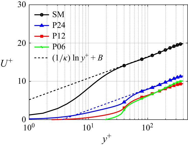
 U+
 y+
 p/k=6,12,24
 U+=(1/κ)lny++B
 κ=0.41
 B=5.2
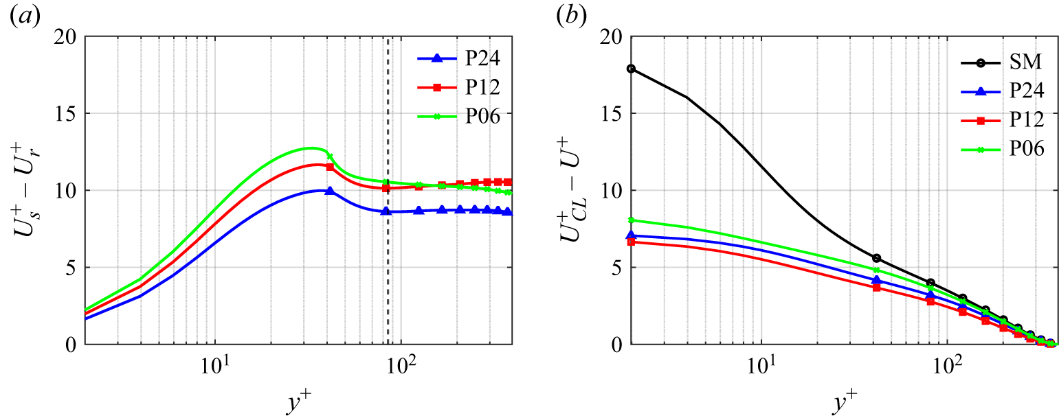
 Us+−Ur+
 y+
 UCL+−U+
 y+≳100
 ΔU+
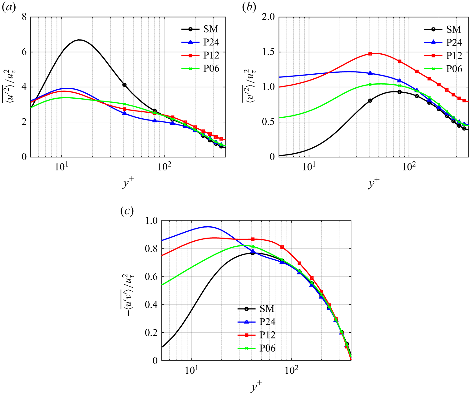
 y+
 ⟨u′2¯⟩/uτ2
 ⟨v′2¯⟩/uτ2
 −⟨u′v′¯⟩/uτ2
 p/k=6,12,24

 lx/h=2.0
 lz/h=0.5
 u/UCL
 um
 uk
 uk≈0.88UCL

 uk/UCL
 lx/h∈[1.0,6.0]
 lz/h∈[0.1,3.0]
 uk/UCL

 u/UCL
 z
 y
 u/UCL=0.95

 um
 uk
 lz/h
 lx/h=2
 lx/h
 lz/h=0.5

 um,1
 um,2
 Um,1
 Um,2
 Uk
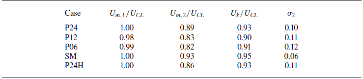
 Um,1
 Um,2
 Uk
 σ2
 um,2

 uk

 u/UCL=0.95
 dc
 x
 y
 z/h=3
 y
 z
 x/h=6

 x
 y
 δc=yu−yl
 yc=(yu+yl)/2

 δc
 yc/h
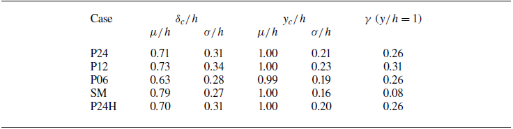
 δc
 yc
 γ
 μ
 σ

 γ
 y/h

 x
 y

 U,u~,u^
 u′2¯,u′~2,u′^2
 l⋅~
 l⋅^
 l⋅¯

 ξ=0
 U/UCL
 Ωz
 ξ

 Q2
 y+≈47
 x
 y
 y
 z

 x
 y
 z+=157.5
 Q2
 y+≈47
 Q4
 y+≈47
 0≤y+≤k+
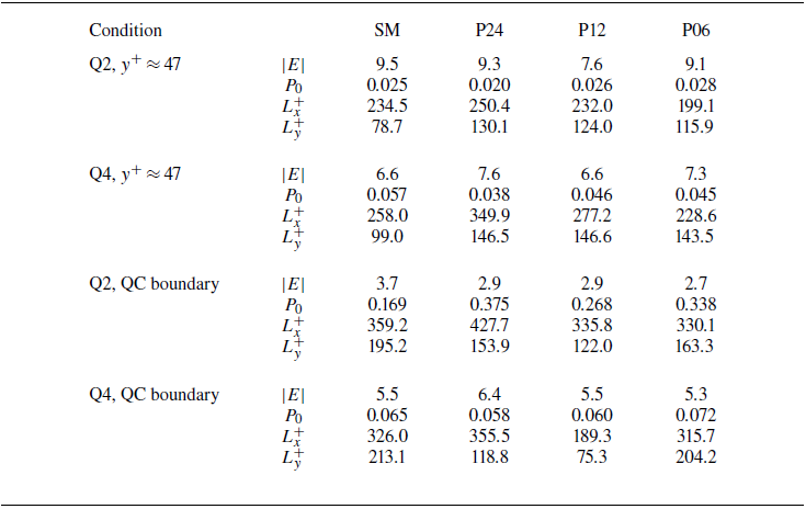
 |E|=α(u∗2+v∗2)1/2
 α=3
 P0
 Lx+
 Ly+
 λci2
 z+=157.5
 5%
 λci2
 2%

 u′v′P(u′,v′)
 Δ=0.01
 [−0.08,−0.02]
 [0.01,0.03]

 y+
 ⟨u′v′⟩Q/⟨u′v′⟩
 ⟨u′v′⟩Q=∬(u′,v′)∈Qu′v′P(u′,v′∣y)du′dv′
 Q2
 Q1
 Q3
 Q4

 ⟨u′v′⟩Q(H)/⟨u′v′⟩
 I(H)=(|u′v′|>H⟨−u′v′⟩)
 Q2
 Q1
 Q3
 Q4
 Q2
 Q3
 Q1
 Q4

 ξ
 ξ=0
 ⟨u′v′⟩Q/⟨u′v′⟩
 Q2
 Q1
 Q3
 Q4

 y+−k+
 τν+
 τR+
 τD+
 τtotal+
 y+−k+=0

 u/UCL
 um
 uk
 u=uk

 uk

 UΣ/UCL
 ξ/h
 ξ/h<−ξfit
 ξ/h>ξfit
 ξ=0
 ΔU
 (∂UΣ/∂ξ)max
 δw
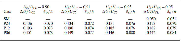
 ΔU/UCL
 δw/h
 Uk/UCL
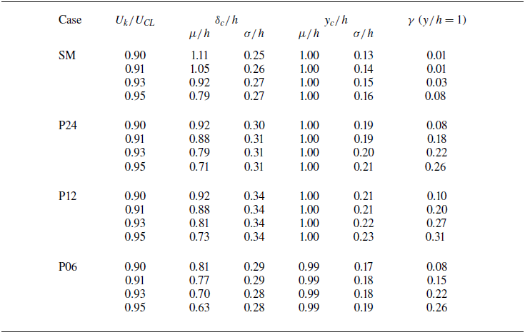
 Uk/UCL
 μ
 σ
 δc
 yc
 γ
 y/h=1
 Uk/UCL=0.95
 0.95
 0.93
 0.90
 0.91

 um,1
 um,2
 Reτ=590

 Reτ=395
 Reτ=590
 δc
 γ
 y/h

 Lx=12h
 Lx=24h

 u/UCL
 x
 y
 Lx=24h
 u/UCL=0.95

 y+≈47
 Lx=12h
 Lx=24h


