Introduction
Streams in Maritime Antarctica show a rapidly changing hydrology during the short summer season determined by meteorological variables and melting processes. Detailed relationships between hydrology, meteorological variables, catchment topography and melting processes, have been recorded in Antarctic streams in the McMurdo Dry Valleys area (McKnight et al. Reference McKnight, Gooseff, Vincent and Peterson2008, Stanish et al. Reference Stanish, Nemergut and McKnight2011). However, differences in stream hydrology can be expected because temperatures and rainfall in Maritime Antarctica are usually higher than on the Antarctic continent (Convey et al. Reference Convey, Bindschadler, Di Prisco, Fahrbach, Gutt, Hodgson, Mayewski, Summerhayes and Turner2009, Rochera et al. Reference Rochera, Justel, Fernández-Valiente, Bañón, Rico, Toro, Camacho and Quesada2010). The daily variability in stream hydrological conditions has been described in Maritime Antarctica following daily insolation cycles, and the water temperatures vary from freezing at night to up to 10°C, closely following the ambient air temperatures (Hawes & Brazier Reference Hawes and Brazier1991, Rochera et al. Reference Rochera, Justel, Fernández-Valiente, Bañón, Rico, Toro, Camacho and Quesada2010).
Stream ecological processes, such as competition, predation, resource acquisition, dispersal and habitat use, are important factors structuring benthic communities (Biggs & Smith Reference Biggs and Smith2002) and controlling benthic algal biomass (Biggs Reference Biggs1996, Luttenton & Baisden Reference Luttenton and Baisden2006). These processes are modulated by macro- and micro-scale variations in stream velocity (Biggs Reference Biggs1996, Peterson Reference Peterson1996, Hart & Finelli Reference Hart and Finelli1999). Changes in stream velocity associated with insolation cycles modify stream chemical and hydrological parameters, which have been found to influence algal assemblages in streams on James Ross Island (Hawes & Brazier Reference Hawes and Brazier1991). Variations in the composition of epilithic algae communities have also been related to variability in water chemistry and stream discharge (Pizarro et al. Reference Pizarro, Izaguirre and Tell1996, Pizarro & Vinocur Reference Pizarro and Vinocur2000) as well as to the periphyton productivity and the seasonal variation of biomass in streams of King George Island (Pizarro & Vinocur Reference Pizarro and Vinocur2000, Elster & Komarek Reference Elster and Komarek2003). Furthermore, stream hydrology was determined to be a relevant factor for understanding the structure and productivity of algal communities in polar streams (Howard-Williams et al. Reference Howard-Williams, Vincent, Broady and Vincent1986, Hawes & Brazier Reference Hawes and Brazier1991, Davey Reference Davey1993, Pizarro & Vinocur Reference Pizarro and Vinocur2000, Stanish et al. Reference Stanish, Nemergut and McKnight2011).
The frequency and intensity of hydrological disturbances caused by floods are fundamental determinants of the spatial patterns of benthic algal biomass and richness (Biggs Reference Biggs1996, Hart & Finelli Reference Hart and Finelli1999, Biggs & Smith Reference Biggs and Smith2002). The frequency of low-flow disturbances impacts community composition and dynamics (Ledger et al. Reference Ledger, Harris, Armitage and Milner2008). Low-flow disturbance events could alter algal assemblages via desiccation or by exposing them to freezing conditions. Certain diatoms are better adapted to surviving dry and/or freezing periods (Souffreau et al. Reference Souffreau, Vanormelingen, Verleyen, Sabbe and Vyverman2010), and others could be protected from desiccation within resistant biofilms (Davey Reference Davey1989). Furthermore, low-magnitude spates when the shear force of water is too low to mobilize coarse bed material but sufficient to mobilize small sand particles by a hopping motion known as saltation (Luce et al. Reference Luce, Steele and Lapointe2010b) could also be a relevant determinant of benthic communities (Luce et al. Reference Luce, Cattaneo and Lapointe2010a). Saltation motion can cause sloughing, scraping and peeling off of attached algal biomass and determines the size and arrangement of periphyton refuge zones across a stream channel (Luce et al. Reference Luce, Steele and Lapointe2010a). Indeed, disturbances caused by suspended loads of solids have been reported to be an important factor that limits periphyton development in polar streams (Howard-Williams et al. Reference Howard-Williams, Vincent, Broady and Vincent1986, Elster & Komarek Reference Elster and Komarek2003). In the context of low-magnitude hydrological disturbances and the presence of refuge zones for stream biota, it would be expected that the substratum type (texture, size), orientation and location in the streambed could play a major role in determining the structure of benthic algal communities. Furthermore, in polar streams, hydrology might determine habitat harshness by promoting desiccation and substrate exposure to colder conditions. Recent reports have shown that endemic Antarctic species are more abundant in harsh habitats, suggesting that Antarctic diatoms are better adapted to these conditions (Esposito et al. Reference Esposito, Horn, McKnight, Cox, Grant, Spaulding, Doran and Cozzetto2006, McKnight et al. Reference McKnight, Gooseff, Vincent and Peterson2008).
The goals of the present study are to assess the role of the substrate type in modulating the effects of hydrology on the development of diatom communities in a typical Maritime Antarctic stream, and to investigate what environmental conditions promote or suppress Antarctic endemic species. The stream studied (Petreles, unofficial name) is located on Byers Peninsula, which is the largest ice-free area of Livingston Island (South Shetland Islands). The area is characterized by a large number of seasonally ice-covered lakes and streams with small catchments, supplied with water from lake outlets or snow and permafrost melting (Toro et al. Reference Toro, Camacho, Rochera, Rico, Bañón, Fernández-Valiente, Marco, Justel, Avendaño, Ariosa, Vincent and Quesada2007, Rochera et al. Reference Rochera, Justel, Fernández-Valiente, Bañón, Rico, Toro, Camacho and Quesada2010). The diatom assemblages in this stream have been analysed since they dominate biofilm communities on all of the substrates (Fernández-Valiente et al. Reference Fernández-Valiente, Camacho, Rochera, Rico, Vincent and Quesada2007, Toro et al. Reference Toro, Camacho, Rochera, Rico, Bañón, Fernández-Valiente, Marco, Justel, Avendaño, Ariosa, Vincent and Quesada2007).
The results of this study can subsequently be used in palaeoecological reconstructions of past environmental and/or climatological variability and in predicting future stream community scenarios under current climate change conditions (Convey et al. Reference Convey, Bindschadler, Di Prisco, Fahrbach, Gutt, Hodgson, Mayewski, Summerhayes and Turner2009). Additionally, polar streams are considered to represent dynamic hotspots in the landscape due to their higher sensitivity to climate change in comparison with terrestrial ecosystems (McKnight et al. Reference McKnight, Gooseff, Vincent and Peterson2008).
Methods
Study area and sampling site
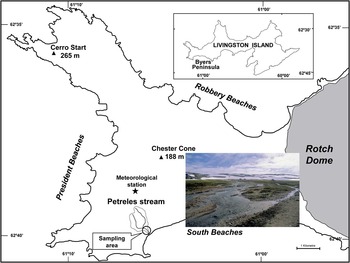
Byers Peninsula forms the western tip of Livingston Island (South Shetland Islands), which is located close to the Antarctic Peninsula (Fig. 1). It is limited on its eastern border by the Rotch Dome ice cap, and the geology of the area is composed of Upper Jurassic–Lower Cretaceous marine sedimentary, volcanic and volcaniclastic rocks. Permafrost is found at a depth of c. 30–100 cm under the active lithosol layer of shattered rocks. The hydrology of the catchment during summer months is mainly influenced by ice and snow melting, rainfall and underground water flows in the active layer over the permafrost. The influence of these underground flows on stream flow generation in polar latitudes has previously been discussed by other authors (Carey & Woo Reference Carey and Woo1998).
Location of Byers Peninsula and the sampling area (Livingston Island) in Antarctica. Inset is a photograph of the sampling site in Petreles stream.

In the Maritime Antarctic region the climate is less extreme than in continental Antarctica, with mean summer temperatures of c. 1–3°C and mean annual precipitation varying between 500 and 800 mm (Bañón et al. Reference Bañón, Justel, Velazquez and Quesada2013). Byers Peninsula is snow-covered for at least 7–8 months a year, with permanent snow packs found in many accumulation areas (Rochera et al. Reference Rochera, Justel, Fernández-Valiente, Bañón, Rico, Toro, Camacho and Quesada2010).
The stream studied (Petreles, unofficial name) is situated in the South Beaches hydrographic basin (62°39′55.26″S, 61°5′52.78″W) and has a catchment area of c. 70 ha. The stream flow regime is mainly pluvio-nival, with maximum flows occurring during summer months. The sampling site was located c. 100 m upstream of the river mouth in South Beaches. The stream here is of the second order and flows through a flat area, corresponding to the middle set of Holocene raised marine features on Byers Peninsula, with a braided channel, generating a large number of marginal shallow areas between central channels. The shores of the fluvial bed along this stream stretch are widely colonized by moss carpets. The stream bed is composed of pebbles of up to 20 cm, gravel and sandy substrate. During low stream discharges after major melting periods, clay deposits are formed in marginal or lentic areas.
Meteorological data
Meteorological data on air temperature were obtained from a Campbell meteorological station installed on the main plateau of Byers Peninsula (c. 65 m above sea level), located c. 1.7 km from the sampling area and less than 1 km from the beginning of the stream. Additional precipitation data were collected during the summer season with a funnel collector.
Stream water analyses
The stream water analyses included measurements of temperature, specific conductance, pH and dissolved oxygen, which were monitored using a YSI 556 MPS water logger system during the entire study period. Stream flows were estimated using a SIGMA PVM 3872 current velocity meter (Doppler system), with measurements taken at different depths in the stream cross-sectional channel area from 8 January 2004 (Julian day 8, JD 8) to 1 February 2004 (JD 32).
Benthic community sampling and microscopic analysis
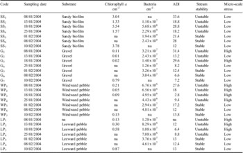
Weekly samples were collected from the beginning of January 2004 to the middle of February 2004 from four different stream substrates: windward pebbles (WP), leeward pebbles (LP), gravel (G) and sandy biofilm (SS), totalling 28 samples (seven x four substrates; Table I). The diameter of the pebbles was c. 15 cm, and that of the gravel was c. 3–5 cm. Both were sampled from a permanently submerged zone in the central flowing channels. Samples of WP were collected from the front of pebbles where the stream flow hit the pebble (flow facing side). Conversely, LP samples were collected on the protected rear side of the pebbles. Finally, sandy samples were collected from the marginal clay-sandy areas of the stream. The sampled area (from 2–10 cm2) was delimited using sticky film for the pebbles and gravel. The biofilm within these delimited opened squares was detached using a toothbrush and washed with a distilled water bottle through a funnel to collect the sample in a polythene bottle. Biofilms from shoreline sand (epipsammon and epipelon) were sampled by collecting the upper 5 mm of the substrate surface with a mini-corer (10 mm in diameter). The final samples consisted of ten homogenized replicates for gravels and five replicates for pebble and sand samples, all of which were preserved with 3% formaldehyde.
Codes for the samples with the sampling date and substrate type, as well as the chlorophyll a and bacterial concentrations. Stream stability period refers to the two main hydrological periods. Micro-scale stress indicates the likely influence of stream velocity on the benthic diatom assemblages.

ADI = Antarctic Diatom Index. na = missing values.
All of the samples were treated with hydrogen peroxide (33% H2O2) and mounted in Naphrax® (R.I. = 1.7, Brunel Microscopes Ltd, UK) following the method described in Battarbee et al. (Reference Battarbee, Jones, Flower, Cameron, Bennion, Carvalho and Juggins2001) for diatom analysis. In each sample, 500 diatom valves were identified and counted in random transects at 1200 x magnification under oil immersion using a Zeiss Axio Imager A1 microscope (Carl Zeiss Inc, Germany) equipped with an 100 x objective (Zeiss Plan-Apo 1.4 numeric aperture) and differential interference contrast (Nomarski®) optics.
The identification of Antarctic species was based on Van de Vijver et al. (Reference Van de Vijver, Frenot and Beyens2002, Reference Van de Vijver, Beyens and Lange-Bertalot2004, Reference Van de Vijver, Zidarova and de Haan2010a, Reference Van de Vijver, Mataloni, Stanish and Spaulding2010b, Reference Van de Vijver, Zidarova, Sterken, Verleyen, de Haan, Vyverman, Hinz and Sabbe2011a, Reference Van de Vijver, Sterken, Vyverman, Mataloni, Nedbalová, Kopalová, Elster, Verleyen and Sabbe2011b), Sabbe et al. (Reference Sabbe, Verleyen, Hodgson, Vanhoutte and Vyverman2003), Esposito et al. (Reference Esposito, Spaulding, McKnight, van De Vijver, Kopalová, Lubinski, Hall and Whittaker2008), Van de Vijver & Mataloni (Reference Van de Vijver and Mataloni2008), Kopalová et al. (Reference Kopalová, Elster, Nedbalová and van De Vijver2009), Zidarova et al. (Reference Zidarova, van de Vijver, Mataloni, Kopalová and Nedbalova2009, Reference Zidarova, van de Vijver, Quesada and de Haan2010), and Van de Vijver & Zidarova (Reference Van de Vijver and Zidarova2011). All valves belonging to different species in the Nitzschia perminuta (Grunow) M. Peragal.-complex were aggregated into one designation: ‘N. perminuta agg.’ Further morphological and taxonomic research will be necessary to establish their correct identity.
Chlorophyll a and bacteria concentration analysis
Chlorophyll a (chl a) was analysed as a measure of biomass. For pebbles and gravels, an aliquot of the samples collected in polythene bottles was filtered through glass fibre filters (GF/F; Whatman). For the biofilms from sand, three cores were collected as described previously and stored in the dark in whirl-pack® bags. All samples were frozen until analysis. Quantification of chl a concentration in the samples was performed using High-performance Liquid Chromatography (HPLC). The pigments were extracted from both GF/F and sand, using acetone via vortexing and sonication. The extracts were filtered through 0.2 μm nylon filters and subsequently injected into a Waters® C18 Spherisorb S5 ODS2 column. All of the injected samples were composed of 50–100 μl of the extracts mixed with a volume of ammonium acetate (IPA: ion pairing agent) to obtain a final IPA concentration of 0.1 mM. The eluted pigments were detected using a diode array detector (PDA Waters 996®) at an absorbance range of 350–750 nm. Chlorophyll a was quantified against the curve obtained using a standard by integration of the area under the cross-section at 440 nm.
The same diatom sampling protocol was used for obtaining bacterial samples, except that the samples were fixed with buffered formalin (4% final concentration) and stored at 4°C until analysis. Bacterial counts were carried out using epifluorescence microscopy on stained material. Prior to staining and slide preparation, an aliquot of the formalin fixed samples was treated with tetra sodium pyrophosphate (PPi) to desorb bacteria from soil particles. Subsequently, the samples were stained with DAPI (4’,6-diamidino-2-phenylindole) for ten minutes and filtered through black polycarbonate filters (0.2 μm) to retain bacteria. During filtration, a 0.8 μm pore-size cellulose acetate backing filter was used to obtain a uniform distribution of cells. The samples were then inspected on a Zeiss-III phase contrast epifluorescence microscope at 1250 x.
Micro-scale physical stress
Micro-scale physical stress is a function of stream discharge (velocity) and substrate type and their relative orientation towards the main flood, which affects scouring, substratum movement and sediment abrasion (Biggs Reference Biggs1996, Peterson Reference Peterson1996, Luce et al. Reference Luce, Steele and Lapointe2010b). Therefore, we assumed that the sandy substratum (SS), which was found in marginal areas of the stream, was a substrate associated with low physical stress. The epilithic samples from the rear of pebbles (LP) are also likely to be a substrate characterized by low physical stress. The substrates that are likely to support higher physical stress are those collected from the front of pebbles (WL) and gravels (G). It is difficult to define physical disturbance in streams, and different views and metrics proposed for this purpose have been a matter of debate (Stanley et al. Reference Stanley, Powers and Lottig2010). We assume that changes in stream velocity and variability imply rapid changes in energy and the transport of materials in suspension, which would affect stream biota to different degrees (Stevenson Reference Stevenson1983, Peterson Reference Peterson1996, Biggs et al. Reference Biggs, Nikora and Snelder2005, Luce et al. Reference Luce, Steele and Lapointe2010b, Stanley et al. Reference Stanley, Powers and Lottig2010). Nevertheless, for ecologists an effective disturbance should have measurable effects on biota. Biomass removal could be used as a measure of disturbance (Stanley et al. Reference Stanley, Powers and Lottig2010). Although we have incomplete data on the chl a concentrations and bacterial biomass for each substrate we suggest that changes in bacteria and chl a concentrations could be an indicator of effective stream disturbances for epilithic communities.
Data analysis
Principal components analysis (PCA) was carried out on the square root-transformed abundance data. Principal components analysis of square root transformed abundance data is identical to using the Hellinger distance between the original row vectors of species abundances, which is a recommended transformation for ordination methods (Legendre & Gallagher Reference Legendre and Gallagher2001). Nevertheless, to test whether a linear (PCA) or a unimodal model (correspondence analysis, which uses a chi-squared distance) was the most appropriate model for analyzing the diatom abundance data, a detrended correspondence analysis (DCA) was carried out to estimate gradient length. The results showed that the total gradient length was less than two SD, indicating a linear relationship (ter Braak & Šmilauer Reference ter Braak and Šmilauer1998). Only diatoms with abundances > 1% in one or more samples were included in the PCA, which was performed using CANOCO 4.5 (ter Braak & Šmilauer Reference ter Braak and Šmilauer1998).
Diatom assemblage diversity was calculated in terms of the species-richness (S) and the exponential of Shannon's entropy (exp(H)), which is more appropriate than classical diversity indices for assessing statistically independent measures of alpha and beta diversity (Jost Reference Jost2007). All diversity measures were calculated following Jost (Reference Jost2007). The exponential of Shannon diversity was calculated as follows:
 $$ \exp (H)\: = \:\exp \left( {{\rm{ - }}\mathop{\sum}\nolimits_{i\:{\rm{ = }}\:{\rm{1}}}^{{S}} {\smallint {{p}_i}\ln \,{{p}_i}} } \right), \eqno\rm$$
where pi is the relative abundance of species i and S is the number of species. For each sampling date the diversity (D) was partitioned into alpha (α), beta (β) and gamma (γ; total diversity) components following Jost (Reference Jost2007).
 $$ D_{\beta }^{q} \: = \:D_{\gamma }^{q} /D_{\alpha }^{q} \eqno\rm$$
where q could be S or exp(H). Beta diversity was used as a measure of the differences in the species composition between substrate types for a given date (Jost Reference Jost2007). The Berger-Parker index was used as a measure of dominance (Magurran Reference Magurran2004). The diatom community turnover (T) between two consecutive samples was calculated for each substrate using a β diversity metric (Dβ, see Eq. (2)) based on the exponential of Shannon entropy (where q = exp(H)) (Jost Reference Jost2007) as follows: T = (Dβ-1)/(2-1), where T ranges from 0 (no turnover between samples) to unity (each sample is completely different from every other sample). All of the analyses were performed using the R statistical program (R v. 2.9.1.; http://www.r-project.org/) and additional functions from the R-packages “vegetarian” v. 1.2, “vegan” v. 1.17-0, and “indicspecies”.
Samples were classified using cluster analysis (hierarchical group average) (Legendre & Legendre Reference Legendre and Legendre1998) in an underlying Hellinger distance similarity matrix to use the same distance metric as in PCA. The Hellinger distance is a recommended measured for clustering and produces results consistent with Bray-Curtis similarity (Legendre & Gallagher Reference Legendre and Gallagher2001). Similarity profile statistical test (SIMPROF) was used to search for statistically significant evidence (P < 0.02) of genuine clusters (Clarke Reference Clarke1993). Analysis of similarities (ANOSIM, 999 permutations) (Legendre & Legendre Reference Legendre and Legendre1998) was applied to test for differences in the diatom assemblages between the stream hydrological phases and substrate types. Both analyses were performed using the PRIMER 6 statistical package (Clarke Reference Clarke1993).
We identified the ecological indicator values for each diatom taxon to assess the ecological preferences among substrates types and clusters. We employed the point-biserial equalised correlation coefficient (r-index), which takes into account the absence of species both inside and outside the site-group combination under investigation. The r-equalised index avoids the potential problem of unbalanced sampling and can detect negative associations (De Cáceres et al. Reference De Cáceres, Legendre and Moretti2010). We took on account all possible combinations of groups of sites and selected the combination for which the species can be best used as indicator (De Cáceres et al. Reference De Cáceres, Legendre and Moretti2010). The Antarctic Diatom Index (ADI) was calculated as the percentage of endemic Antarctic diatoms in each sample (Esposito et al. Reference Esposito, Horn, McKnight, Cox, Grant, Spaulding, Doran and Cozzetto2006).
Results
Meteorology and hydrology
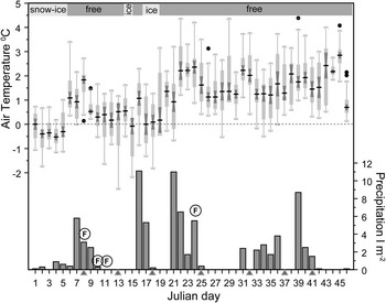
Data from the meteorological station installed on the Byers Peninsula were obtained from 1 January 2004 (JD 1) to 15 February 2004 (JD 46). The daily air temperatures were mainly above freezing after JD 20 (Fig. 2). This relatively warm period started with a period of rain, which removed large amounts of snow from the stream catchment. Close to its outlet in South Beaches, Petreles stream showed velocity values between 0.26 and 2.33 m s-1. However, velocity data were only collected from JD 8–JD 29. The daily fluctuations measured during a sunny day in January (JD 19) fluctuated between 0.26 and 2.33 m s-1, and the water discharge fluctuated between 0.048 and 0.948 m3 s-1. The highest discharge rate (2.33 m3 s-1) was recorded on JD 11 after a warm period between JD 6 and JD 11 when the air temperatures were continuously above 0°C (Fig. 2). This large amount of discharge was related to a rapid thaw of the snowfields in the stream catchment area. Unfortunately, due to technical problems, we missed a second large stream discharge on JD 24, which was also related to a warm period when there was rain. The stream discharge after this flood was quite constant (from 0.08–0.13 m3 s-1). However, the minimum water discharge (0.048 m3 s-1) was recorded on JD 19 during a cold period (JD 18–JD 19) with mean temperatures below 0°C (Fig. 2). Snow and ice cover on the stream were recorded during two main periods: before the first sampling date (JD 8) and before and during the third sampling date (JD 18). These samples were collected with ice and/or snow covering Petreles stream (Fig. 2).
Environmental climate conditions throughout the sampling period. Boxplot of the daily air temperatures. Grey bars denote amount of precipitation per day. (F) indicates high stream flows. Triangles indicate sampling dates.

Based on the above results and field observations, we defined two phases of variability in Petreles stream: 1) early summer (from JD 1–JD 24), which is an unstable phase, when there are large fluctuations in the stream flow, related to the main thawing season, when there are successive freezing and thawing events, and 2) late summer, which is a stable phase with air temperatures that are almost constantly above freezing and the stream's catchment includes few or absent snow fields.
Diatom community composition
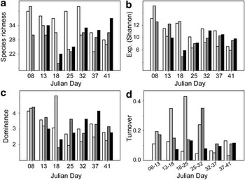
We identified 87 diatom taxa from 27 samples (unfortunately the first sample from leeward pebbles (LP1) was missing). The total number of taxa varied between the substrates (sand = 65, gravel = 58, windward pebbles = 55, leeward pebbles = 58; ANOVA F = 3.27, P < 0.05). The diversity (exp(H)) and species-richness varied throughout the sampling period but were relatively stable after an initial decreasing phase for all substrate types, with the exception of species-richness in the sand samples, which decreased in the last two samples (Fig. 3a & b). The changes in diversity parallel the changes in dominance (Figs 3c & 4). The specific substrate community turnover between consecutive samples showed an overall higher stability in samples from the rear of pebbles (LP) and sandy biofilms (SS). Higher turnover was observed in gravels (between G3 and G4) and in epilithic assemblages from the front face of stones (between WP4 and WP5) (Fig. 3d). The differences in turnover between the studied substrates (Fig. 3d) are indicative of differences in the stability of the diatom assemblages on each substrate type. Interestingly, all of the diatom assemblages showed low turnover in late summer (Fig. 3d).
Measures of a. species-richness (S), b. diversity (exp), c. dominance, and d. community turnover for each substrate type. White bars denote sandy samples, light grey bars denote gravel samples, dark grey bars denote windward pebbles, and black bars denote leeward pebbles.

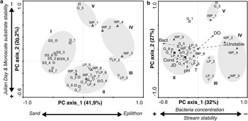
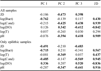
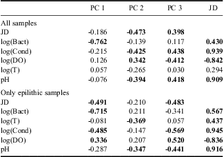
The main component of diatom variability (PC 1) explained 42% of the total variability and clearly differentiated all of the sand assemblages (SS) from the epilithic assemblages (G, WP and LP). The second component (PC 2) explained 20.2% of the variability in the diatom assemblages and was mainly related to changes in epilithic assemblages (Fig. 5a). PC 2 was correlated with JD (Table II), which indicated a temporal trend in the diatom communities throughout the sampling period. However, the JD could co-vary with a number of other environmental variables showing temporal trends such as pH, conductivity and dissolved oxygen (Table II). To analyse the epilithic diatom communities without the influence of sandy samples on the main axis of variability, a second principal component analysis (PCAepi) was carried out. We observed similar clusters of samples (Fig. 5b) in the previous PCA carried out with all samples (PCAall). The main component explained 32% of the total diatom assemblage variability and was correlated with JD and conductivity (Table II). However, as in previous PCAall, the concentration of bacteria showed a higher correlation with the main component (Table II). Furthermore, samples from late summer define a similar cluster as in PCAall (Fig. 5a & b).
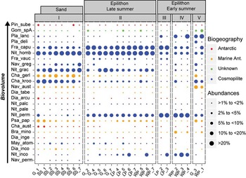
Dot blot representation of relative diatom abundance counts (only species > 1%). Boxes separate samples by cluster (see Fig. 6). Species are arranged according to their biovolume. Samples are coded following Table I. Nav_perm = Navicula perminuta, Nit_inco = Nitzschia inconspicua, Dia_inco = Diadesmis inconspicua, May_atom = Mayamea atomus, Dia_inge = Diadesmis ingeae, Bra_mino = Brachysira minor, Cha_aust = Chamaepinnularia australomediocris, Psa_pap = Psammonthidium papilio, Nit_perm = Nitzschia perminuta agg., Nit_pale = Nitzschia palea, Nit_palc = Nitzschia paleacea, Dia_arcu = Diadesmis arcuata, Dia_tabe = Diadesmis tabellariaeformis, Nav_aust = Navicula australoshetlandica, Cha_kroo = Chamaepinnularia krookiformis, Cha_gerl = Chamaepinnularia gerlachei, Nit_grac = Nitzschia gracilis, Nav_greg = Navicula gregaria, Fra_vauc = Fragilaria cf. vaucheriae, Nit_homb = Nitzschia homburgensis, Fra_capu = Fragilaria capucina s.l., Pla_deli = Planothidium delicatulum, Pla_lanc = Planothidium lanceolatum, Gom_spA = Gomphonema spA, Pin_sube = Pinnularia sub-Antarctica var. elongata.

Principal component analysis (PCA) biplot. The symbols for the samples denote the substrate type: circles represent sand samples, squares represent gravel samples, upward triangles represent the windward side of pebbles, downward triangles represent the leeward side of pebbles. Sample names are given in Table I. The light grey oval delimits samples from clusters classification shown in Fig. 6. a. The results of the PCA for all of the sampled diatom assemblages. b. The results of the PCA for the epilithic assemblages only. In b. black symbols denote samples added to the PCA as passive samples due to the lack of bacterial data. Environmental variables were included in the PCA as additional data and therefore did not constrain the ordination results.

Correlation coefficients between the three main components of the variability of the diatom assemblages (PC 1, PC 2 & PC 3) and the environmental variables. JD = Julian day, Bact = the bacterial concentration, Cond = conductivity, DO = dissolved oxygen, T = water temperature. Statistically significant correlations are shown in bold (P < 0.05).
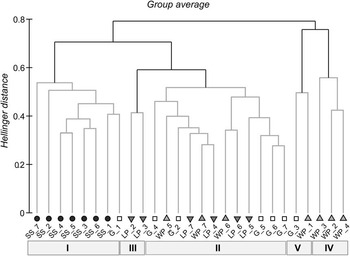
The cluster analysis classified samples into five different statistically significant groups (based on SIMPROF results, P < 0.02; Fig. 6). Cluster I separated all of the sandy biofilm samples plus the first gravel sample (G1) from the other samples. Cluster II contained all of the epilithic samples from the late summer, when there was higher hydrological stability, except for one sample from the front of pebbles (WP4). Cluster III was adjacent to cluster II, and contained two samples from early summer, but from the hydrologically protected rear of pebbles (LP2 and LP3). Cluster IV and cluster V were exclusively comprised of early summer samples from the front of pebbles (from WP1–WP4), with the exception of one gravel sample (G3). This gravel sample together with WP1 constituted cluster V. These clusters reflected the structure of the diatom assemblages (PCA in Fig. 5), which were related mainly to changes among the dominant species (Fig. 4).
Results of hierarchical cluster analysis (group average) based on the Hellinger distance similarity index. Sample names and symbols as in Fig. 3 and Table I. Cluster names are given in Roman numerals (I–V). The light grey dendrogram branches denote branches with no remaining structure (SIMPROF test; P < 0.02).

Although the analysis of diatom assemblage similarity (ANOSIM) indicated differences between the substrates types (global test R = 0.42; P < 0.001; 999 permutations), the pairwise values of the R statistic indicated that these differences were only due to large differences between assemblages from the shoreline sandy biofilms and the epilithic samples. Interestingly, ANOSIM of all epilithic samples indicated significant differences in the diatom assemblages between the two phases of stream stability (global test R = 0.34; P < 0.001; 999 permutations). Indeed, all of the late summer (after JD 24) epilithic assemblages (WP5–WP7, LP4–LP7, G4–G7) showed higher similarity than the early summer epilithic assemblages (Figs 4 & 5).
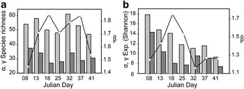
Finally, the overall diversity (γ diversity, based on exp(H)) showed a decreasing trend throughout the sampling period (Fig. 7a), while the γ diversity based on S did not show a clear trend (Fig. 7b). Beta diversity was used as a measure of the similarity among the diatom assemblages on each sampling date. However, we observed two different patterns (Fig. 7a & b). The β diversity based on exp(H) decreased after a large increase on JD 18 and remained low after JD 24, which represented the division between the two hydrological phases (early vs late summer) (Fig. 7b). In contrast the β diversity based in S did not show a clear trend. Similar results were observed for γ and α diversity based in S (Fig. 7a). Beta diversity metric based in S is more sensitive to changes in species with low abundances (satellite species) than β diversity based in the exp(H).
Measures of alpha (α), beta (β) and gamma (γ) diversity based on a. the species-richness, and b. Diversity (Exp(H)) for each sampling date from Julian day 8 (JD 8) to Julian day 41 (JD 41). Dark grey bars represent α diversity, light grey bars represent γ diversity, and the line scatter plot represents β diversity.

Diatoms with indicator value
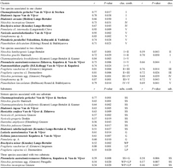
The r-index (species indicator value) identified indicative species for each substrate type (Table III). Several of the species showing significant indicator value exhibit a strictly Antarctic distribution, and some of them are even restricted to the Maritime Antarctic region, such as Chamaepinnularia gerlachei, Navicula australoshetlandica, Eolimna jamesrossensis and Diadesmis cf. ingeae (Kopalová & Van de Vijver Reference Kopalová and van de Vijver2013). These endemic Antarctic species showed a high indicator value for sandy biofilms and for the substrates that were more likely to be disturbed during high stream flow events (gravel and windward pebbles samples). Interestingly, following the classification of diatom species into three ecological guilds (Passy Reference Passy2007), species from sandy microbial mats, gravel and windward pebbles belong to the motile guild, whereas two cosmopolitan species of Fragilaria that belong to the high profile guild were associated with the protected side of pebbles (Table III).
Results of the indicator species analysis. For each species, we indicate the cluster or substrate that showed the highest correlation (clus. comb. or subs. comb.), the value of the correlation (r) and the statistical significance (P-value). For patterns including more than one cluster or substrate, we also indicate the results obtained for the most highly related single cluster or substrate when combinations are not considered (clus. or subs.). Cluster and substrates codes are defined in the main text. Endemic Antarctic species are presented in bold. Pinnularia sp. A, Gomphonema sp. A and Gomphonema sp. B are undescribed taxa. SS = sandy biofilm, G = gravel, WP = windward pebble, LP = leeward pebble.

The r-index was also calculated based on cluster classification. Two cosmopolitan species (Nitzschia homburgensis, Nitzschia gracilis) were associated and dominated cluster II (Table III, Fig. 4), which consisted of a group of late summer epilithic samples from the hydrologically stable phase in the stream. Both species are relatively fast moving species (motile guild). However, Antarctic species (i.e. N. australoshetlandica, Pinnularia parakolbei, Psammonthidium papilio and Brachysira minor) were indicative of cluster V and cluster IV (Table III) from the early summer period. The species associated with the front of pebbles (WP) during early summer (cluster IV) were all small species (B. minor, Nitzschia inconspicua and N. perminuta (Table III, Fig. 4). Finally, the species associated with the rear of pebbles (LP) during early summer (cluster III) were mainly from the high profile guild, including Fragilaria capucina and Fragilaria vaucheriae cf.
Measures of biomass
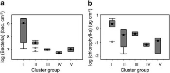
Despite the restricted number of samples analysed to determine chl a and bacterial concentration (Table I), the two proxies of epilithic biomass showed similar patterns (Fig. 8). As expected, the sandy samples showed the highest values, and among all of the epilithic substrate samples, those from the late summer (cluster II) showed the highest values. Low values of chl a and biomass correspond to clusters from the early summer period (Fig. 8).

Antarctic Diatom Index and diversity
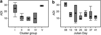
The ADI value patterns were similar to the biomass measures (Fig. 9a), but a higher mean ADI was recorded for epilithic samples from the early colonization (cluster V and Table I). Higher ADI variability also corresponds to the early summer period. The greatest variability in ADI values between substrates was recorded on JD 18 (Fig. 9b, Table I), after/during a period in which the stream was frozen (Fig. 2), while lower values were recorded in the pebble samples (6%). We found that a high percentage of endemic species correspond to a higher diversity (exp(H)) (linear model: r 2 = 0.819; P < 0.0001). However, a quadratic model fit was slightly better than a linear model for the species-richness (linear: r 2 = 0.490; P < 0.0001; quadratic: r 2 = 0.494; P < 0.0001).
Boxplot of the Antarctic Diatom Index (ADI) for a. each cluster, and b. each sampling date.

Discussion
Although no remarkable relationships have been found between daily stream discharges and mean daily temperatures in different Antarctic areas such as the McMurdo Dry Valleys (McKnight et al. Reference McKnight, Gooseff, Vincent and Peterson2008), in the South Shetland Islands (Deception Island), stream discharge has been observed to be associated with the air temperature (Inbar Reference Inbar1995). The hydrology of Antarctic meltwater streams is mainly determined by the seasonal and daily heat balance in catchment snow and ice rather than by rainfall (McKnight et al. Reference McKnight, Gooseff, Vincent and Peterson2008). Indeed, precipitation events exhibit a low intensity on Byers Peninsula (Rochera et al. Reference Rochera, Justel, Fernández-Valiente, Bañón, Rico, Toro, Camacho and Quesada2010) (Fig. 2). In Petreles stream, the discharges also increased during warm periods (temperatures above 0°C), especially in the early summer, when there were large snowfields in the stream catchment area. During the late summer, however, after several days of air temperatures above 0°C, the stream flow showed low variability and never froze. This lack of change occurs because after the main thawing period, snowfields were scarce in the Petreles stream catchment area. The absence of glaciers means that the stream cannot be fed with melting water throughout the entire summer. The source of stream flow during late summer is mainly from the active layer, which plays a role as a “surface aquifer” that collects water from rainfall, dispersed snow packs and progressively releases water to the stream network. Therefore, large stream discharges were absent during late summer.
Diatoms are present in low densities in cyanobacterial mats in other Maritime Antarctic localities, but they can represent up to 30% of the biomass in Livingston Island streams close to the study site (Davey Reference Davey1993). Indeed, diatoms dominated the stream biofilm in the South Beaches basin on Byers Peninsula (Fernández-Valiente et al. Reference Fernández-Valiente, Camacho, Rochera, Rico, Vincent and Quesada2007). Hence, the changes in diatom communities could be representative of the changes in the overall stream algal biofilm community. The relationship between the early and late summer hydrological phases and the diatom community structure can be illustrated by dividing the sampling period in two categories. Indeed, the distinctive patterns in early vs late summer β diversity based in exp(H) (Fig. 7b) indicate a large shift in the dominant species between the two hydrological seasons. The early summer diatom assemblages were dominated by N. perminuta agg., but the late summer assemblages were dominated by N. homburgensis (Fig. 4). However, ordination and cluster analysis showed a finer structure related to the sampling date (JD), as well as to the substrate type, which merits further analysis (Figs 4, 5 & 6). Our results suggest a strong relationship between diatom communities and small-scale hydrological conditions. Benthic algal communities were strongly influenced by hydrological regimes and shear stress in Arctic, Antarctic streams and elsewhere (Stevenson Reference Stevenson1983, Howard-Williams et al. Reference Howard-Williams, Vincent, Broady and Vincent1986, Elster & Komarek Reference Elster and Komarek2003, Biggs et al. Reference Biggs, Nikora and Snelder2005, Stanish et al. Reference Stanish, Nemergut and McKnight2011). Furthermore, substrate type and size and the localization of substrates with respect to the main stream flow modulate the ecological effects of hydrological disturbances on benthic organisms at different spatial and temporal scales (Stevenson Reference Stevenson1983, Biggs Reference Biggs1996, Peterson Reference Peterson1996, Hart & Finelli Reference Hart and Finelli1999, Biggs et al. Reference Biggs, Nikora and Snelder2005, Luttenton & Baisden Reference Luttenton and Baisden2006, Luce et al. Reference Luce, Steele and Lapointe2010b).
Whilst we did not observe large spates in Petreles stream, a high frequency of low discharges could be sufficient to cause ecological changes (Doyle et al. Reference Doyle, Stanley, Strayer, Jacobson and Schmidt2005). The effective discharge related to periphyton accumulation in Sycamore Creek was only 0.67 m3 s-1 (Doyle et al. Reference Doyle, Stanley, Strayer, Jacobson and Schmidt2005). Higher values of up to 0.95 m3 s-1 were recorded in Petreles stream during early summer associated with thawing and raining events. Furthermore, the frequency and distribution of low-flow disturbances determine the community composition and dynamics (Ledger et al. Reference Ledger, Harris, Armitage and Milner2008, Luce et al. Reference Luce, Steele and Lapointe2010b, Stanish et al. Reference Stanish, Nemergut and McKnight2011). In Petreles stream, daily fluctuations (high frequency) in velocity and discharge were recorded, and this could therefore be sufficient to affect epilithic communities. Low-magnitude spates are sufficient to mobilize small sand particles via saltation (Luce et al. Reference Luce, Steele and Lapointe2010b), which could cause sloughing, scraping and peeling off of the attached algal biomass. This phenomenon determines the size and arrangement of periphyton refuge zones across the stream channel (Luce et al. Reference Luce, Steele and Lapointe2010b) and control the development of benthic communities (Luce et al. Reference Luce, Cattaneo and Lapointe2010a). The concentrations of bacteria and chl a (Fig. 8), as proxies of effective disturbance, showed a trend toward higher values in the late summer epilithic samples. A similar pattern was found for the diatom assemblages (i.e. via cluster classification or PCA ordination).
These results suggest that small high frequency hydrological fluctuations could control the structure of stream diatom communities, but with substrate orientation and type also playing a role. In the PCA, it was observed that one of the main axes of variability is related to the JD and bacterial concentration (Table II, Fig. 5), which could be related to substrate biomass. Nevertheless, Antarctic sites exhibit contrasting seasons that result in a strong seasonal signal (e.g. with respect to air and water temperatures, light intensity and quality and water chemistry). Other stream physical and chemical parameters such as pH and conductivity changed monotonically throughout the season and were correlated with JD (Table II). These environmental parameters are also important environmental variables explaining diatom assemblages (Battarbee et al. Reference Battarbee, Jones, Flower, Cameron, Bennion, Carvalho and Juggins2001), and changes in stream algal resources are often associated with changes in stream discharge (Pizarro et al. Reference Pizarro, Izaguirre and Tell1996, Biggs & Smith Reference Biggs and Smith2002, Biggs et al. Reference Biggs, Nikora and Snelder2005). Whilst we could not reject an additional role for water chemistry, the difference between substrates could not be explained by these large-scale stream processes associated with changes in water chemistry and resources. In theory, on a given sampling date, all of the epilithic substrates were surrounded by the same stream water. Therefore, the observed differences among the substrates and sampling days (e.g. Fig. 5) should be related to processes at a micro-scale that modulate the availability of resources and energy over each substrate (Biggs & Smith Reference Biggs and Smith2002, Biggs et al. Reference Biggs, Nikora and Snelder2005).
Diatom traits at a micro-scale
The late summer diatom assemblages (cluster II) showed high similarity between substrate types (Fig. 4). During this period when the stream flow was more stable than in early summer we recorded high values of the bacterial biomass and chl a (Fig. 8). The community turnover was low throughout the late summer (Fig. 3), and the diatom community was dominated by large and highly motile species (Nitzschia spp.) (Table III). Motility is an important trait when resources such as light are limiting in a large (high biomass) biofilm mat. However, some substrates, such as the rear of pebbles (cluster III), exhibited the late summer “archetypical” community before the front of pebbles (cluster IV). These results indicate the importance of small-scale processes, such as the saltation (Luce et al. Reference Luce, Steele and Lapointe2010b) and mass transfer (Biggs et al. Reference Biggs, Nikora and Snelder2005), that are related to substrate orientation in controlling the development of the late summer diatom community. Interestingly, the ecological traits of diatoms associated with the front (cluster IV) vs the rear of pebbles (cluster III) in early summer were very distinctive. The front was dominated by small-sized diatoms (Fig. 4, Table II), which are characterized by rapid growth. This is expected to be a positive trait in an energetic environment such as the front of a pebble, where populations could be reduced by successive spates and/or saltation dynamics (Luce et al. Reference Luce, Steele and Lapointe2010b). In contrast, the rear was dominated by large species with a high surface/volume ratio and belonging to the high profile guild such as Fragilaria spp. (Fig. 4). This difference between the two sides of the same pebble could be a result of a trade-off between energy uptake and energy conversion to produce offspring, with large species being superior in terms of resource acquisition and small species being superior in the conversion of resources into reproductive processes (Brown et al. Reference Brown, Marquet and Taper1993). At this small-scale, the two sides of a pebble would show differences in mass transfer (e.g. resources availability) and drag-disturbance processes (Biggs et al. Reference Biggs, Nikora and Snelder2005). As expected diatoms from the low profile guild such as Planothidium lanceolatum reached maximum abundance in environments with a higher shear stress (clusters IV and V) (Passy Reference Passy2007).
Micro-scale habitat heterogeneity related to the differential effects of flow variability on the different sampled substrates could explain the higher dissimilarity observed between the diatom assemblages during the unstable period in the stream compared to the stable period (Fig. 5). However, greater environmental instability could also increase the role of additional factors, such as the random arrival and establishment of propagules (Stevenson Reference Stevenson1983, Hart & Finelli Reference Hart and Finelli1999), substrate size (Luttenton & Baisden Reference Luttenton and Baisden2006, Parker & Huryn Reference Parker and Huryn2011), and species variability with respect to resisting freezing and desiccation events (Davey Reference Davey1989, Souffreau et al. Reference Souffreau, Vanormelingen, Verleyen, Sabbe and Vyverman2010) in determining differences among diatom assemblages. Interestingly, epilithic samples from the initial phase (cluster V) showed high diversity and low dominance, but in turn, they showed high similarity to the sandy biofilm samples (Fig. 4). This result suggests that the diatom assemblages from cluster V represent an initial colonization phase, which is likely to occur after major removal of algae due to sediment scouring (abrasion) during flow disturbance events or trough gravel turnover, when free substrate would be available to be colonized. The similar diatom community structure found in the first gravel sample, which consisted of ten homogenized replicates (see Methods), and the first sandy sample suggest that the sandy assemblages were a main source of new propagules. However, both assemblages could also be influenced by new diatom arrivals during a high flow event. Indeed, all of the samples from the first sampling date (JD 8) showed higher homogenization (low β diversity) in the composition of rare species as indicated by the lower β diversity value (based in S) of JD 8 samples (Fig. 7a). A strong community homogenization is likely to occur after a large stream flood during early summer. Large floods could be expected when air temperatures rise above 0°C in early summer, when the stream catchment is covered by large amounts of snow and the thawing season starts. In contrast, the low β diversity value observed on the last sampling date (Fig. 7a), can be attributed to high stream stability, which tends to homogenize stream diatom assemblages from different substrates. Unfortunately, we do not have biomass data from all the samples to fully support these two contrasting hypotheses for the two sampling dates.
The sandy biofilm samples were the most differentiated ones of the collected samples, with their diatom assemblages showing high temporal stability and diversity/richness. These assemblages showed only minor differences between the two periods of stream stability. These algal biofilms were located on sandy stream shorelines, meaning that they were less subject to being influenced by the stream disturbance regime than the epilithic communities located in the main stream channel. A low intensity and frequency of disturbances would facilitate the growth and maintenance of a structured biofilm, thus determining internal resource gradients, providing more opportunities for species co-existence and easing negative interspecific interactions (Larson & Passy Reference Larson and Passy2012). Previous studies of stream mat communities on Livingston Island showed similar results. The diatom composition during summer showed fewer differences in lentic areas (where mats are well developed) than in lotic habitats (Davey Reference Davey1993). However, the high diversity of these sandy biofilms could also be a consequence of alluvial deposition, which would explain the dominance of highly motile species, such as N. homburgensis and Chamaepinnularia spp. throughout the summer season (Fig. 4). Therefore, the chance of new species arriving and becoming established are higher on shoreline beaches than in highly disturbed zones, such as epilithic substrate where species might arrive easily, but have difficulty becoming established (Stevenson Reference Stevenson1983, Hart & Finelli Reference Hart and Finelli1999). The resulting complex structure and the environmental stability of these species-rich shoreline biofilms mean that they act as an effective seed bank containing “seeds” that are ready to grow when a new growing season arrive. This process would be similar to a terrestrial vegetation seed response when the optimal growing season arrives, which plays a major role in maintaining species diversity, such as via storage effects (Chesson Reference Chesson2000). Further research should be performed to assess whether these shoreline mats provide better overwinter conditions for diatom species.
Diversity and ADI relationship
Apparently, Antarctic diatom species are better adapted to the harsh environment of the region (with dry and freezing periods) than cosmopolitan species (Esposito et al. Reference Esposito, Horn, McKnight, Cox, Grant, Spaulding, Doran and Cozzetto2006, McKnight et al. Reference McKnight, Gooseff, Vincent and Peterson2008), although Stanish et al. (Reference Stanish, Nemergut and McKnight2011) related high ADI values to the abundance of well-adapted Luticola and Hantzchia species to hydrologically variable, low-flow environments. The diatom assemblages from the initial colonization phase (cluster V) were characterized by a high diversity (lower dominance) and abundance of endemic Antarctic diatoms species, such as N. australoshetlandica. The dominance of these species resulted in high ADI values. The sandy shoreline algal biofilms also showed high ADI and diversity values and their diatom assemblages were similar to those of cluster V (Fig. 4). These results suggest that sandy biofilms are the main supply of Antarctic diatoms propagules, which were able to colonize “free” epilithic environments when summer arrived.
The stronger relationship between ADI and species diversity than between ADI and species-richness suggested an important role of dominance in controlling the former relationship. We found that the dominant species were mainly cosmopolitan species. Therefore, lower dominance in a diatom community results in high ADI values. However, if Antarctic species were dominant, high ADI values could decrease species diversity due to the exclusion of widespread species (Esposito et al. Reference Esposito, Horn, McKnight, Cox, Grant, Spaulding, Doran and Cozzetto2006).
The role of climate
The significant warming detected on the Antarctic Peninsula (Convey et al. Reference Convey, Bindschadler, Di Prisco, Fahrbach, Gutt, Hodgson, Mayewski, Summerhayes and Turner2009) could have consequences for stream communities. Minor changes in the climate conditions in the Byers Peninsula area where summer temperatures are close to 0°C (Rochera et al. Reference Rochera, Justel, Fernández-Valiente, Bañón, Rico, Toro, Camacho and Quesada2010, Bañon et al. 2013), are likely to change the balance between early summer and late summer stream hydrology. Extending late summer hydrological conditions due to higher temperatures in early summer would involve large changes in diatom stream assemblages but could also involve changes in the stream population of endemic species. During late summer, Antarctic diatom species were outcompeted by cosmopolitan species (N. homburgensis, Fig. 4). The sandy biofilms showed a lower diversity and lower ADI values during late summer, while epilithic samples showed a greater number of Antarctic species during the early summer, hydrologically unstable phase in the stream (Fig. 4). So minor changes in the duration of stream hydrological conditions could also have consequences for the population of Antarctic species and their diversity. A shortening summer season with air temperatures that are always about 0°C and successive short periods of freezing and thawing, would favour the dominance of cluster V assemblages, which exhibit a higher abundance of endemic species (N. australoshetlandica, Pinnularia australomicrostauron and Psammonthidium papilio) (Table III, Fig. 4). Furthermore, the warmer temperatures could, in turn, cause a large number of the streams in Byers Peninsula to dry up during a long summer season and, could therefore damage diatoms from sandy biofilms due to desiccation. Several endemic species were associated with the sandy biofilms, such as C. gerlachei, Diadesmis ingeae and P. australomicrostauron (Table III, Fig. 4). In addition, mild (cold) winters could select different diatom species (Parker & Huryn Reference Parker and Huryn2011) by changing the overwintering stream flooding conditions (McKnight et al. Reference McKnight, Gooseff, Vincent and Peterson2008).
Interestingly, diatom assemblages from some lakes on Byers Peninsula that are entirely fed by glacial meltwater streams are dominated by similar endemic species (Kopalová & Van de Vijver Reference Kopalová and van de Vijver2013) to the stream species from clusters I, IV & V (Table III). These clusters mainly come from the early summer period when the stream showed higher hydrological variability, including daily fluctuations in discharge and freezing conditions. The discharge of small streams, which are fed by glacial meltwater, can vary as much as tenfold during a single day as a result of the changing insolation and sun angle (McKnight et al. Reference McKnight, Gooseff, Vincent and Peterson2008). The dominance of some of these lotic species in sedimentary records and their variability could be used as indicators of past hydrological conditions and therefore of climate conditions. This framework of stream communities exhibiting sensitivity to summer climate variability linked to stream hydrological conditions and the sensitivity of the Antarctic Peninsula to climate variability (Convey et al. Reference Convey, Bindschadler, Di Prisco, Fahrbach, Gutt, Hodgson, Mayewski, Summerhayes and Turner2009) means that diatoms records from sedimentary oligotrophic environments with low internal productivity, such as lakes and ponds, are important archives of past climate conditions and early sentinels of present climate change.
Conclusions
The present study contributes to the understanding of the importance of the stream physical environment for structuring diatom assemblages. The seasonal variability in these assemblages is modulated by micro-scale erosional and depositional processes related to the substrate type, orientation regarding the main stream flow, and position on the stream bed. The epilithic diatom assemblages from late summer were stable and showed higher similarity between the investigated substrate types but were dominated by motile cosmopolitan species. The diatoms assemblages from sandy biofilms exhibited the highest stability and did not show large changes in their composition and structure between the two stream hydrological periods. These biofilms presented a higher diversity with a large number of endemic species. Although further work is needed to confirm this hypothesis, sandy biofilms could be the main source of propagules for epilithic substrates when the growing season starts. In this context, sandy biofilms would represent an important component for maintaining diatom diversity in Antarctic freshwater ecosystems.
Stream hydrology is ultimately a function of the climate, consequently, Antarctic freshwater ecosystems are highly relevant for monitoring and predicting future climate change because they integrate the fluxes and cycles of water, sediment and solutes in their catchments and from the surrounding landscape, including terrestrial ecosystems. Obtaining a better understanding of species’ ecological preferences as well as a well-defined taxonomy is essential for studying, reconstructing, predicting and mitigating the effects of climate change in the Earth's ecosystems.
Acknowledgements
This study was supported by the Spanish Ministry of Science and Technology through LIMNOPOLAR projects (REN2000-0435-ANT and CGL2005-06549-C02-01/ANT to AQ, as well as CGL2005-06549-C02-02/ANT to AC, with the last being co-financed by European FEDER funds), which are aimed at investigating aquatic ecosystem responses under different environmental conditions and to predicting their sensitivity to climate variability. This article was published thanks to the financial support given by the Ministerio de Ciencia e Innovación (Spain) (CTM2011-12973-E). The authors are indebted to Dr Ana Justel and Dr Annick Wilmotte (LIMNOPOLAR Team) for their help with the fieldwork, as well as to Vicente Marco (UTM-CSIC) and the Spanish Navy (Las Palmas crew) for logistical support. The constructive comments of the reviewers are also gratefully acknowledged.