


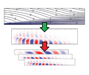

1. Introduction
Resolvent analysis allows investigation of dominant coherent structures in time-invariant flows (Trefethen et al. Reference Trefethen, Trefethen, Reddy and Driscoll1993; Schmid & Henningson Reference Schmid and Henningson2001; McKeon & Sharma Reference McKeon and Sharma2010). The governing equations derived from linearizing the Navier–Stokes equations around the temporal mean, however, include an unknown term, the coherent component of the Reynolds-stress tensor. This unknown term generally occurs when considering linearized equations of turbulent flows and can be interpreted as the effect of fine-scale turbulence on the large-scale coherent structures resolved by the linear model (Reynolds & Hussain Reference Reynolds and Hussain1972; del Álamo & Jiménez Reference del Álamo and Jiménez2006; Wu & Zhuang Reference Wu and Zhuang2016). By analogy with the Reynolds-averaged Navier–Stokes (RANS) equations, the coherent component of Reynolds stresses is typically modelled using a Boussinesq approach, which relates the term to the coherent strain-rate tensor via an effective eddy viscosity (Reynolds & Hussain Reference Reynolds and Hussain1972; del Álamo & Jiménez Reference del Álamo and Jiménez2006). This leaves the eddy viscosity as the only modelling parameter. The use of eddy viscosity for modelling the coherent part of the Reynolds-stress tensor in linear analysis has evolved over the last decades. In the following we will briefly summarize a few selected studies.
McKeon & Sharma (Reference McKeon and Sharma2010) include all nonlinear terms in the forcing vector in their pipe flow resolvent analysis, which implies that the coherent component of Reynolds stresses is not explicitly modelled. This approach is also followed for the resolvent analysis of the turbulent flow around a NACA 0012 airfoil (Thomareis & Papadakis Reference Thomareis and Papadakis2018). Wu & Zhuang (Reference Wu and Zhuang2016) investigate the nonlinear interaction of large-scale coherent structures in a free shear layer and model the influence of the coherent component of the Reynolds stresses using a Boussinesq model with eddy viscosity. In their nonlinear model, which treats the interaction of coherent structures as organized motion, the influence of eddy viscosity (fine-scale turbulence) is found to be small. In linear stability analysis of turbulent mean-fields, the coherent component of the Reynolds-stress tensor is also often neglected (Iungo et al. Reference Iungo, Viola, Camarri, Porté-Agel and Gallaire2013; Mettot, Sipp & Bézard Reference Mettot, Sipp and Bézard2014). However, the inclusion of eddy viscosity in linear analysis has proven advantageous in recent years, as shown, for example, in Crouch, Garbaruk & Magidov (Reference Crouch, Garbaruk and Magidov2007), Moarref & Jovanović (Reference Moarref and Jovanović2012), Viola et al. (Reference Viola, Iungo, Camarri, Porté-Agel and Gallaire2014), Tammisola & Juniper (Reference Tammisola and Juniper2016), Rukes, Paschereit Oliver & Oberleithner (Reference Rukes, Paschereit Oliver and Oberleithner2016), Oberleithner, Paschereit & Wygnanski (Reference Oberleithner, Paschereit and Wygnanski2014) and Mantič-Lugo & Gallaire (Reference Mantič-Lugo and Gallaire2016).
This finding has recently also been adopted for resolvent analysis. Eddy viscosity augmented resolvent analysis is based on the premise of considering the influence of turbulence, which is represented by the coherent component of the Reynolds-stress tensor, via the dissipative Boussinesq model so that the resolvent forcing vector is reduced to the energetic non-dissipative component. For example, Schmidt et al. (Reference Schmidt, Towne, Rigas, Colonius and Brès2018) apply resolvent analysis with an effective Reynolds number corresponding to a spatially constant eddy viscosity to investigate coherent structures in jets in the subsonic, transonic and supersonic regimes. Maia et al. (Reference Maia, Heidt, Pickering, Colonius, Jordan and Brès2024) investigate the effect of flight on coherent structures in a turbulent jet based on eddy viscosity-augmented resolvent analysis. Morra et al. (Reference Morra, Semeraro, Henningson and Cossu2019) and Symon, Illingworth & Marusic (Reference Symon, Illingworth and Marusic2021) apply the Cess (Reference Cess1958) eddy viscosity model to augment the resolvent operator and investigate coherent structures in turbulent channel flows. Coherent structures in the far-field of a round turbulent jet are analysed based on local stability and resolvent analyses with eddy viscosity in Kuhn, Soria & Oberleithner (Reference Kuhn, Soria and Oberleithner2021). These studies show that resolvent analysis enables modelling of coherent structures with a high level of agreement with reference data when the dissipative effects of turbulence are explicitly accounted for by the eddy viscosity.
Although the use of eddy viscosity in linear stability analysis and resolvent analysis is now widespread, the modelling approaches used differ considerably. Schmidt et al. (Reference Schmidt, Towne, Rigas, Colonius and Brès2018) interpret the effective Reynolds number (spatially constant eddy viscosity) as a free model parameter and select a value that leads to good results compared with an available database. Another common approach is to calibrate an eddy viscosity based on the turbulence statistics. This involves inversion of the Boussinesq model based on known Reynolds stresses and the mean strain-rate tensor (Rukes et al. Reference Rukes, Paschereit Oliver and Oberleithner2016; Tammisola & Juniper Reference Tammisola and Juniper2016; Kuhn et al. Reference Kuhn, Soria and Oberleithner2021). By assimilating the RANS equations to large-eddy simulation (LES) mean-fields, an eddy viscosity can be determined without knowledge of the Reynolds stresses (von Saldern et al. Reference von Saldern, Reumschüssel, Kaiser, Sieber and Oberleithner2022, Reference von Saldern, Reumschüssel, Kaiser, Schmidt, Jordan and Oberleithner2023). Symon et al. (Reference Symon, Madhusudanan, Illingworth and Marusic2023) and Viola et al. (Reference Viola, Iungo, Camarri, Porté-Agel and Gallaire2014) calibrate constants in eddy viscosity models based on literature and measured data, respectively. Mons, Vervynck & Marquet (Reference Mons, Vervynck and Marquet2024) assimilate a RANS model including a Spalart–Allmaras turbulence model to particle image velocimetry (PIV) measurements. These approaches, which are based on a data-driven calibration of an eddy viscosity (turbulence) model, additionally allow fluctuations in eddy viscosity to be taken into account in the linear model (Crouch et al. Reference Crouch, Garbaruk and Magidov2007).
Towne, Schmidt & Colonius (Reference Towne, Schmidt and Colonius2018) and Lesshafft et al. (Reference Lesshafft, Semeraro, Jaunet, Cavalieri and Jordan2019) established a direct link between spectral proper orthogonal decomposition (SPOD) and resolvent analysis. In case of a spatially uncorrelated forcing, resolvent and SPOD modes are identical. Inspired by this theoretical insight, Pickering et al. (Reference Pickering, Rigas, Schmidt, Sipp and Colonius2021) adjust the eddy viscosity through data-driven optimization, using the alignment between resolvent and SPOD modes of a jet flow as the cost function to be optimized. For the axisymmetric mode it is shown that with this approach a very high degree of alignment with the SPOD modes can be achieved over the considered frequency range.
The objective of the present work is not to achieve the highest possible alignment in the largest possible parameter space, but rather to understand the role of eddy viscosity in resolvent analysis of broadband turbulent flows. Without this understanding, it is not possible to find suitable predictive eddy viscosity models that do not require prior knowledge of the coherent structures to be modelled. To this end, we take a data-driven approach and consider the SPOD modes of a fully turbulent jet at  $Re=50\,000$ and a Mach number of
 $0.4$ as ground truth for the resolvent model. Moreover, we identify the coherent component of the Reynolds-stress tensor for modes with high-gain separation based on an extended SPOD (eSPOD) approach. The further procedure is largely inspired by the work of Cho, Hwang & Choi (Reference Cho, Hwang and Choi2018), Symon et al. (Reference Symon, Madhusudanan, Illingworth and Marusic2023) and Kuhn et al. (Reference Kuhn, Müller, Knechtel, Soria and Oberleithner2022), who analyse the energy budget of individual coherent structures, separated by frequency and wavenumber. We follow this approach and use not only the global measure of alignment for comparison between SPOD and resolvent modes, but rather take a deep look into the physics of the structures by considering their local energy budget. This allows us to reveal the role of eddy viscosity in resolvent analysis of turbulent jets from an energetic point of view. In the resolvent analysis we consider different viscosities, pure molecular viscosity, a mean-field-consistent eddy viscosity which is assimilated from the mean-field and the RANS equations, and two data-driven eddy viscosities which are determined directly from the identified coherent component of the Reynolds-stress tensor. In this study, we focus on a turbulent jet flow, but the presented methods can be directly applied to other broadband flows to investigate the role of eddy viscosity in their linear analysis.
The remainder of the study is structured as follows. First, we introduce the LES database of the jet flow along with the SPOD and eSPOD methods in § 2. The methods are used to extract coherent structures including the coherent component of Reynolds stresses from the data. This is followed by a brief introduction to resolvent analysis in § 3, the methodology to model the coherent structures in the broadband flow based on the temporal mean state. We then present the energy equation for individual coherent structures in § 4. In § 5, we present different eddy viscosity modelling approaches. In § 6, the different eddy viscosities are analysed in isolation with respect to their ability to represent the energy term associated with the coherent component of the Reynolds stresses. This is followed by § 7, in which we compare the energy budget of resolvent and SPOD modes and discuss the role of eddy viscosity. Finally, the results are summarized and key conclusions are drawn.
2. Data-driven analysis
We start with a short section on the LES database, followed by a section on the data-analysis methods SPOD and eSPOD that are applied to extract the coherent structures and correlated, coherent Reynolds stresses from the broadband data.
2.1. Large-eddy simulation database
The study is based on an LES data set of a jet flow at Reynolds number  $UD/\nu =50\,000$ and Mach number of
 $U/a=0.4$, where
 $U$ and
 $a$ denote the centreline velocity and speed of sound at the nozzle exit,
 $D$ the nozzle diameter and
 $\nu$ the viscosity. The computational domain is based on an experimental set-up and includes a converging nozzle and the jet (Maia et al. Reference Maia, Jordan, Cavalieri, Martini, Sasaki and Silvestre2021; Nekkanti et al. Reference Nekkanti, Maia, Jordan, Heidt, Colonius and Schmidt2022). The boundary layer inside the nozzle is tripped 2.5 diameters upstream of the outlet. For the following analyses, the data is considered in a cylindrical region extending from the nozzle outlet up to 30 diameters downstream and 6 diameters in the radial direction. A total of 10 000 snapshots with a non-dimensional time step of
 $\Delta t = 8.336 \times 10^{-2}$ are considered. The simulation was performed using the solver CharLES. For numerical details we refer the interested reader to Brès et al. (Reference Brès, Ham, Nichols and Lele2017, Reference Brès, Jordan, Jaunet, Le Rallic, Cavalieri, Towne, Lele, Colonius and Schmidt2018). In the following, all quantities are non-dimensionalized with
 $U$ and
 $D$. Consequently, frequencies
 $f$ are given as Strouhal numbers
 ${\rm St}=fD/U$. Figure 1 shows the time- and azimuthal-averaged mean velocity field in the domain of interest. Streamlines and the contour of the mean axial velocity component are shown.
The time- and azimuthal-averaged jet flow velocity mean-field in the domain of interest. Mean velocity streamlines are shown as black lines with arrows, the contour in the background shows the axial velocity component  $\bar {u}_x/U$.

The Reynolds decomposition is applied to separate the velocity fields  $\boldsymbol {u} = [u_x,u_r,u_\theta ]$ into a temporal mean (denoted with bar) and a fluctuating (denoted with prime) component such that
 $\boldsymbol {u} = \bar {\boldsymbol {u}} + \boldsymbol {u}'$. The fluctuating Reynolds-stress tensor is given as
 $\boldsymbol {R}'=\boldsymbol {u}'\otimes \boldsymbol {u}' - \overline {\boldsymbol {u}'\otimes \boldsymbol {u}'},$ with the outer product denoted with the
 $\otimes$-symbol.
2.2. Spectral proper orthogonal decomposition
In order to extract coherent structures from the broadband turbulent flow we apply SPOD (Picard & Delville Reference Picard and Delville2000; Schmidt et al. Reference Schmidt, Towne, Rigas, Colonius and Brès2018); SPOD is similar to space-only POD (Lumley Reference Lumley1970; Berkooz, Holmes & Lumley Reference Berkooz, Holmes and Lumley1993), but extends the methodology to frequency space. For the analysis of the jet flow snapshots the fluctuating velocity component as well as the fluctuating Reynolds stresses are first decomposed into a Fourier series in the periodic azimuthal direction
 $$\begin{gather} \hat{\boldsymbol{u}}_m'(x,r,t) = \mathcal{F}(\boldsymbol{u}'(x,r,\theta,t)), \end{gather}$$
 $$\begin{gather}\hat{\boldsymbol{R}}_m'(x,r,t) = \mathcal{F}(\boldsymbol{R}'(x,r,\theta,t)), \end{gather}$$
where  $\mathcal {F}$ denotes the discrete Fourier transform operator and
 $m$ the real valued azimuthal wavenumber. Due to the periodicity,
 $m$ is an integer. This yields two-dimensional Fourier modes for each time step,
 $\hat {\boldsymbol {u}}_m'$ and
 $\hat {\boldsymbol {R}}_m'$, respectively. Large-scale dominant coherent structures can only be observed for broadband jet flows at low wave numbers. Since modelling large-scale coherent structures is the objective of this study, we limit our analysis to the
 $m=0$ (axis symmetric) and
 $m=1$ mode.
The 10 000 snapshots of the velocity Fourier modes  $\hat {\boldsymbol {u}}_m'$ are divided into
 $N_b$ blocks of 256 snapshots each, where the blocks overlap with
 $50\,\%$. Each block is transformed into Fourier space. For a given azimuthal wavenumber and temporal frequency the matrix
 \begin{equation} \hat{\boldsymbol{U}}_{m,\omega} = [ \hat{\boldsymbol{u}}_{m,\omega}^{(1)}, \hat{\boldsymbol{u}}_{m,\omega}^{(2)}, \hat{\boldsymbol{u}}_{m,\omega}^{(3)},\ldots,\hat{\boldsymbol{u}}_{m,\omega}^{(N_b)} ] \end{equation}
is constructed where  $\hat {\boldsymbol {u}}_{m,\omega }^{(n)}$ denotes the Fourier velocity mode at azimuthal order
 $m$, temporal frequency
 $\omega$ and block
 $n$. From
 $\hat {\boldsymbol {U}}_{m,\omega }$ the sample cross-spectral density matrix can be computed, whose eigenvectors are the SPOD modes. However, we consider here the entire domain extending 6 diameters in the radial direction and 30 diameters in the axial direction, discretized with 138 and 656 points, respectively. The total number of degrees of freedom is therefore much larger than the number of blocks
 $N_b$, which makes the computation of the SPOD modes via the method of snapshots much less expensive. This involves first solving the eigenvalue problem
 \begin{equation} \hat{\boldsymbol{U}}_{m,\omega}^H \boldsymbol{W} \hat{\boldsymbol{U}}_{m,\omega} \boldsymbol{\varPsi} = \boldsymbol{\varPsi} \boldsymbol{\varLambda},\end{equation}
where the superscript  $H$ denotes the complex conjugate transpose and
 $\boldsymbol {W}$ is a weight matrix that takes the volume of each cell into account. The
 $j$th SPOD velocity mode
 $\hat {\boldsymbol {\upsilon }}^{(j)}_{m,\omega }$ follows from expanding the Fourier modes with the
 $j$th eigenvector
 \begin{equation} \hat{\boldsymbol{\upsilon}}^{(j)}_{m,\omega} = \hat{\boldsymbol{U}}_{m,\omega} \boldsymbol{\psi}^{(j)}, \end{equation}
where  $\boldsymbol {\psi }^{(j)}$ denotes the
 $j$th column (eigenvector) of
 $\boldsymbol {\varPsi }$. In total, the decomposition provides
 $N_b$ SPOD modes for each azimuthal order and frequency, which can be ranked according to modal energy content which is represented by the magnitude of the corresponding eigenvalue
 $\lambda ^{(j)}$. Applied to velocity data, the eigenvalue is a measure of the kinetic energy of the mode. Low-rank dynamics, also known as high-gain separation, are present when one mode has a particularly high energy in a given frequency range compared with the others. The dynamics of the flow is then dominated by one coherent structure in the corresponding frequency range. For more information we refer to the guide to SPOD by Schmidt & Colonius (Reference Schmidt and Colonius2020).
Figure 2 shows the SPOD spectrum of the jet flow velocity data for  $m=0$ (figure 2a) and
 $m=1$ (figure 2b). A high gain separation can be observed for
 $m=0$ at intermediate frequencies and for
 $m=1$ at low frequencies. For a more detailed investigation on the energy content of the leading SPOD mode, we show the energy share of each mode in figure 3. It can be observed, that around
 ${St}=0.5$ the flow is dominated by a
 $m=0$ mode and between
 ${St}=0.2\unicode{x2013}0.4$ by a
 $m=1$ mode, both containing approximately 20 % of the total kinetic energy at the corresponding wavenumber.
The SPOD spectrum of the broadband jet flow for  $m=0$ (a) and
 $m=1$ (b). The eigenvalue of the first (leading) mode is shown in black, eigenvalues of subleading modes are shown in graduating shades of grey.

Energy share of the SPOD modes for  $m=0$ (a) and
 $m=1$ (b). The energy share of the leading mode is shown in black, for subleading modes in graduating shades of grey.

2.3. Identification of the coherent component of Reynolds stresses based on eSPOD
In regions of high-gain separation, we hypothesize that the coherent structure has sufficient amplitude to extract information on the higher-order statistics, and in particular the coherent Reynolds stresses. Specifically, we are interested in the part of the Reynolds-stress fluctuation that interacts with the dominant coherent structure. We refer to this as the coherent component of the Reynolds-stress tensor. For a broadband flow, it is difficult to extract this quantity from the data as it is of comparatively low amplitude compared with the coherent structure. We thus identify the coherent Reynolds-stress component by using the same eigenvectors as in (2.4) to also expand Fourier-blocks of the Reynolds-stress fluctuations. This method is also known as eSPOD (Boree Reference Boree2003).
For this purpose, the 10 000 snapshots of Reynolds-stress Fourier modes  $\hat {\boldsymbol {R}}_m'(x,r,t)$ analogue to the velocity modes are first divided into
 $N_b$ blocks, transformed into frequency space and stacked into a matrix for each frequency and azimuthal order
 \begin{equation} \hat{\boldsymbol{O}}_{m,\omega} = [ \hat{\boldsymbol{R}}_{m,\omega}^{(1)}, \hat{\boldsymbol{R}}_{m,\omega}^{(2)}, \hat{\boldsymbol{R}}_{m,\omega}^{(3)},\ldots,\hat{\boldsymbol{R}}_{m,\omega}^{(N_b)} ], \end{equation}
where  $\hat {\boldsymbol {R}}_{m,\omega }^{(n)}$ denotes the blockwise Fourier mode of the fluctuating Reynolds-stress component. In the second step, the Fourier modes are expanded with the same eigenvectors
 $\boldsymbol {\psi }^{(j)}$ as in (2.4),
 \begin{equation} \hat{\boldsymbol{\varGamma}}^{(j)}_{m,\omega} =\hat{\boldsymbol{O}}_{m,\omega} \boldsymbol{\psi}^{(j)}. \end{equation}
Since the eigenvectors were calculated on the basis of velocity data, the approach guarantees extraction of only the part of the Reynolds-stress tensor that is correlated with the corresponding coherent structure (mode  $j,m,\omega$). The following analysis will focus on frequencies between
 ${St}=0.1$ and
 $1$. However, following our reasoning above, caution should be taken when considering results that are based on eSPOD outside of the low-rank region, see figure 3.
In the context of this study, we want to investigate the dominant coherent structures and are therefore only interested in the most energetic mode ( $j=1$). For the sake of clarity, we drop the superscripts and subscripts and only refer to the velocity SPOD mode as
 $\hat {\boldsymbol {u}}_{{S}}$ and the corresponding coherent Reynolds-stress component as
 $\hat {\boldsymbol {R}}_{{S}}$ in the following. The frequency and wavenumber are always given in context.
As an example, figure 4 shows the real part of the axial velocity SPOD mode (figure 4a) and the corresponding real part of the eSPOD axial-radial component of the coherent Reynolds-stress tensor (figure 4b) for  $m=0$ and
 ${St}=0.56$. The axial velocity mode corresponds to the well known Kelvin–Helmholtz mode, which dominates the dynamics of the jet in this frequency range (Pickering et al. Reference Pickering, Rigas, Nogueira, Cavalieri, Schmidt and Colonius2020). The axial-radial component of the coherent Reynolds-stress tensor computed based on eSPOD shows a higher noise level, however, a clear mode shape can be observed, especially in the region where the velocity mode has a high amplitude.


3. Resolvent analysis
We here introduce resolvent analysis, which will be used as a model for the dominant coherent structures. For this purpose, we consider the transport equation of the fluctuating velocity component that is derived by inserting the Reynolds decomposition into the Navier–Stokes equations and subtracting the temporal mean
 \begin{equation} \frac{\partial {\boldsymbol{u}}'}{\partial t}={-}(\bar{{\boldsymbol{u}} }\boldsymbol{\cdot}\boldsymbol{\nabla}) {\boldsymbol{u}}'-({\boldsymbol{u}}'\boldsymbol{\cdot}\boldsymbol{\nabla}) \bar{{\boldsymbol{u}} } - \frac{1}{\rho}\boldsymbol{\nabla} p' + \nu\boldsymbol{\nabla}^2{\boldsymbol{u}}' - \boldsymbol{\nabla}\boldsymbol{\cdot}\underbrace{( {\boldsymbol{u}}' \otimes {\boldsymbol{u}}' -\overline{{\boldsymbol{u}}' \otimes {\boldsymbol{u}}'} )}_{\boldsymbol{R}'} . \end{equation}
Since the Mach number of 0.4 is relatively low, we assume incompressibility. The last term in (3.1) contains the fluctuating Reynolds-stress tensor  $\boldsymbol {R}'$. In the next step, a normal mode ansatz is introduced for all fluctuating quantities,
 \begin{equation} z'(x,r,\theta,t) = \hat{z} (x,r) \exp{(\mathrm{i}m\theta - \mathrm{i}\omega t)}, \end{equation}
where  $\mathrm {i}$ denotes the imaginary unit and
 $\hat {z}$ is the complex amplitude in frequency space. Substituting this ansatz in (3.1) yields
 \begin{equation} -\mathrm{i} \omega \hat{{\boldsymbol{u}}} + (\bar{{\boldsymbol{u}} }\boldsymbol{\cdot}\boldsymbol{\nabla}) \hat{{\boldsymbol{u}} }+(\hat{{\boldsymbol{u}} }\boldsymbol{\cdot}\boldsymbol{\nabla}) \bar{{\boldsymbol{u}} } + \boldsymbol{\nabla}\hat{q} - \nu \boldsymbol{\nabla}^2 \hat{{\boldsymbol{u}}} + \boldsymbol{\nabla}\boldsymbol{\cdot} \hat{\boldsymbol{D}} = \boldsymbol{0} , \end{equation}
where the complex amplitude of the fluctuating Reynolds-stress tensor, that is referred to as the coherent component of Reynolds stresses, is divided into its deviatoric and spherical parts,  $\hat {\boldsymbol {R}} = \hat {\boldsymbol {D}} + \frac {2}{3}\hat {k} \boldsymbol {I}$. The latter contains the coherent kinetic energy
 $\hat {k} = 0.5 (\widehat {u_x' u_x'}+\widehat {u_r' u_r'}+\widehat {u_\theta ' u_\theta '})$ and represents a normal stress. Thus, the spherical part can be absorbed by the pressure forming the modified pressure
 $\hat {q} = \hat {p}/\rho + 2/3 \hat {k}$. The deviatoric part of the coherent component of Reynolds stresses is typically modelled using the Boussinesq model
 \begin{equation} \hat{\boldsymbol{D}} \approx{-} \varTheta [\boldsymbol{\nabla} + \boldsymbol{\nabla}^{\rm T}] \hat{{\boldsymbol{u}}} ={-} \varTheta \hat{\boldsymbol{S}}. \end{equation}
The model relates the deviatoric part of the coherent component of Reynolds-stress tensor via an effective viscosity  $\varTheta$ to the fluctuating strain-rate tensor
 $\hat {\boldsymbol {S}}$. We have dedicated a separate section to the various modelling approaches for
 $\varTheta$ below. However, it should be mentioned here that these modelling choices are motivated by the idea that the energetic dissipation of a coherent structure in terms of its energy transfer to other scales can be described by an eddy viscosity. An energetic consideration of this modelling approach follows in § 4. Substituting the Boussinesq ansatz into (3.3) yields
 \begin{equation} -\mathrm{i} \omega \hat{{\boldsymbol{u}}} + (\bar{{\boldsymbol{u}} }\boldsymbol{\cdot} \boldsymbol{\nabla}) \hat{{\boldsymbol{u}} }+(\hat{{\boldsymbol{u}} }\boldsymbol{\cdot}\boldsymbol{\nabla}) \bar{{\boldsymbol{u}} } + \boldsymbol{\nabla}\hat{q} - \boldsymbol{\nabla}\boldsymbol{\cdot}\left[ (\nu + \varTheta) \hat{\boldsymbol{S}} \right] = \hat{\boldsymbol{f}} , \end{equation}
where terms that result from the remaining part of the coherent Reynolds-stress tensor, which is not considered in the Boussinesq model, are represented by the forcing vector  $\hat{\boldsymbol{f}}$. Equation (3.5) is supplemented by the continuity condition
 $\boldsymbol {\nabla }\boldsymbol {{\cdot }}\hat {{\boldsymbol {u}}} = 0$. Using a discretization scheme the equations can be rearranged in the form
 \begin{equation} \left[ \hat{\boldsymbol{u}}, \hat{q} \right]^{\rm T} = \mathcal{R} \hat{\boldsymbol{f}}, \end{equation}
where  $\mathcal {R}$ denotes the resolvent operator for a given azimuthal wavenumber and frequency.
Equation (3.6) can be interpreted in different ways. For a given forcing in the momentum balance  $\hat{\boldsymbol{f}}$, the corresponding linear response of the flow can be determined in the form of velocity and pressure response modes. However, we are interested here in the structures that are naturally most excited in the flow in order to establish comparability with the data-driven dominant SPOD modes. For this purpose, a singular-value decomposition of the resolvent operator is performed
 \begin{equation} \mathcal{R} = \boldsymbol{V} \boldsymbol{\varSigma}\boldsymbol{F}^H, \end{equation}
that leads to a set of forcing  $\boldsymbol {F}$ and response modes
 $\boldsymbol {V}$, the latter are referred to as the resolvent modes in the following. Here
 $\boldsymbol {\varSigma }$ is a diagonal matrix that contains the singular values. The resolvent mode of the largest singular value
 $\sigma ^{(1)}$ corresponds to the coherent structure, i.e. the structure most strongly amplified by linear mechanisms. This is best illustrated by considering (3.7) for one resolvent mode only
 \begin{equation} \sigma^{(j)} \underbrace{[\hat{\boldsymbol{w}}^{(j)}, \hat{{g}}^{(j)}]^{\rm T}}_{\hat{\boldsymbol{r}}^{(j)}} = \mathcal{R} \hat{\boldsymbol{f}}^{(j)}, \end{equation}
where  $\hat{\boldsymbol{f}}^{(j)}$ and
 $\hat {\boldsymbol {r}}^{(j)}$ are the resolvent forcing and response modes (columns of
 $\boldsymbol {F}$ and
 $\boldsymbol {V}$) that correspond to the singular value
 $\sigma ^{(j)}$. With
 $\hat {\boldsymbol {w}}^{(j)}$ and
 $\hat {{g}}^{(j)}$ we distinguish between the velocity and pressure response mode. Equation (3.8) illustrates that large singular values correspond to strongly amplified structures. A comparison of (3.8) with (3.6) shows that the set of forcing
 $\hat{\boldsymbol{f}}^{(j)}$ and scaled response modes
 $\sigma ^{(j)}\hat {\boldsymbol {r}}^{(j)}$ are also a solution to the transport equation of coherent structures, (3.5). In the context of this work we are only interested in the leading resolvent-forcing mode pair. For the sake of clarity we refer to the scaled leading resolvent velocity response mode as
 $\hat {{\boldsymbol {u}}}_{R} = \sigma ^{(1)}\hat {\boldsymbol {w}}^{(1)}$ and to the corresponding forcing mode as
 $\hat{\boldsymbol{f}}_{R}$.
Using the theoretical connection with the leading SPOD mode (Towne et al. Reference Towne, Schmidt and Colonius2018; Lesshafft et al. Reference Lesshafft, Semeraro, Jaunet, Cavalieri and Jordan2019), which identifies the dominant coherent structure in a natural flow in a data-driven way, the modes modelled with the resolvent analysis are compared with SPOD modes in § 7. Resolvent modes are identical to SPOD modes if the true forcings that result in the SPOD modes as resolvent response modes (called expansion coefficients  $\beta _j$ in Towne et al. (Reference Towne, Schmidt and Colonius2018)) are uncorrelated. The idea behind the use of eddy viscosity is to include nonlinear energy transfer into the resolvent operator, leaving less interaction to be modelled by the resolvent optimal forcing vectors. This is based on the expectation that in this way the true forcings (resolvent expansion coefficients) are less strongly correlated and the resolvent response modes therefore show a higher degree of agreement with the SPOD modes. To calculate the resolvent modes, we use our in-house software FELiCS (Kaiser et al. Reference Kaiser, Demange, Müller, Knechtel and Oberleithner2023), a finite-element solver based on FEniCSx (Baratta et al. Reference Baratta, Dean, Dokken, Habera, Hale, Richardson, Rognes, Scroggs, Sime and Wells2023).
4. Energy budget of coherent structures
The Boussinesq eddy viscosity model in the RANS equations was formulated to model the energy dissipation of the mean flow due to interaction with turbulence. Resolvent analysis models coherent structures at discrete frequencies and wavenumbers based on the temporal mean state. To better understand the role of eddy viscosity for modelling the coherent Reynolds-stress tensor in this framework, we consider the energy balance of individual coherent structures in the following. In order to investigate the energy transfer of individual structures, consideration of the energy balance is a common method, which has recently been considered especially for channel flows (Cho et al. Reference Cho, Hwang and Choi2018; Muralidhar et al. Reference Muralidhar, Podvin, Mathelin and Fraigneau2019; Symon et al. Reference Symon, Illingworth and Marusic2021) but also for the far-field region of a jet flow (Kuhn et al. Reference Kuhn, Müller, Knechtel, Soria and Oberleithner2022). A more detailed derivation of the equation can be found in the corresponding references, here we only describe an abbreviated derivation. Equation (3.3) is first multiplied by  $\hat {{\boldsymbol {u}}}^*$, and the resulting equation then integrated over a control volume
 \begin{align} \int -\mathrm{i} \omega |\hat{{\boldsymbol{u}}}|^2 \,\mathrm{d}\varOmega &={-} \int \hat{{\boldsymbol{u}}}^* \boldsymbol{\cdot} (\bar{{\boldsymbol{u}} }\boldsymbol{\cdot}\boldsymbol{\nabla}) \hat{{\boldsymbol{u}}} \,\mathrm{d}\varOmega - \int \hat{{\boldsymbol{u}}}^* \boldsymbol{\cdot} (\hat{{\boldsymbol{u}}}\boldsymbol{\cdot}\boldsymbol{\nabla}) \bar{{\boldsymbol{u}} } \,\mathrm{d}\varOmega - \int \hat{{\boldsymbol{u}}}^* \boldsymbol{\cdot}\boldsymbol{\nabla}\hat{q} \,\mathrm{d}\varOmega \nonumber\\ &\quad + \int \hat{{\boldsymbol{u}}}^* \boldsymbol{\cdot} \nu \boldsymbol{\nabla}^2 \hat{{\boldsymbol{u}}} \,\mathrm{d}\varOmega + \int \boldsymbol{\nabla}\hat{{\boldsymbol{u}}}^* \boldsymbol{\cdot}\hat{\boldsymbol{D}} \,\mathrm{d}\varOmega, \end{align}
where  $\,^*$ denotes the complex conjugate and
 $|\hat {{\boldsymbol {u}}}|^2 = \hat {{\boldsymbol {u}}}^* \boldsymbol {{\cdot }} \hat {{\boldsymbol {u}}}$ is the kinetic energy of a coherent structure. Here
 $\varOmega$ denotes the two-dimensional axial-radial spatial domain. In the last term we exploited the divergence theorem. The boundary integral vanishes assuming all fluctuations to be zero at the domain boundaries. If the real part of (4.1) is considered, the term on the left-hand side vanishes which means that the integrated energy of the coherent structure neither increases nor decreases in time. This yields a balance of the various energy terms (Muralidhar et al. Reference Muralidhar, Podvin, Mathelin and Fraigneau2019; Symon et al. Reference Symon, Madhusudanan, Illingworth and Marusic2023) for each coherent structure separated by frequency
 $\omega$ and azimuthal wavenumber
 $m$,
 \begin{equation} \int \hat{{C}} +
\hat{{P}} + \hat{{Q}} + \hat{{D}}_\nu + \hat{{N}}
\,\mathrm{d}\varOmega = 0
\end{equation}
with
 $$\begin{gather} \hat{{C}} ={-}{\rm Re} \left( \hat{{\boldsymbol{u}}}^* \boldsymbol{\cdot}(\bar{{\boldsymbol{u}} }\boldsymbol{\cdot} \boldsymbol{\nabla}) \hat{{\boldsymbol{u}}} \right), \end{gather}$$
 $$\begin{gather}\hat{{P}} ={-}{\rm Re} \left( \hat{{\boldsymbol{u}}}^* \boldsymbol{\cdot} (\hat{{\boldsymbol{u}}}\boldsymbol{\cdot}\boldsymbol{\nabla}) \bar{{\boldsymbol{u}}} \right), \end{gather}$$
 $$\begin{gather}\hat{{Q}} ={-}{\rm Re} \left( \hat{{\boldsymbol{u}}}^* \boldsymbol{\cdot} \boldsymbol{\nabla} \hat{q} \right), \end{gather}$$
 $$\begin{gather}\hat{{D}}_\nu ={+}{\rm Re} \left( \hat{{\boldsymbol{u}}}^* \boldsymbol{\cdot} \nu \boldsymbol{\nabla}^2 \hat{ \boldsymbol{{\boldsymbol{u}}}} \right), \end{gather}$$
 $$\begin{gather}\hat{{N}} ={+}{\rm Re} \left( \boldsymbol{\nabla}\hat{{\boldsymbol{u}}}^* \boldsymbol{\cdot}\hat{ \boldsymbol{D}} \right). \end{gather}$$
The remaining terms in the energy balance of the individual coherent structures, (4.2) and (4.3), are the following: a convection term  $\hat {{C}}$, that represents the energy transfer due to mean-field convection. The quantity
 $\hat {{P}}$ represents an energetic interaction term with the temporal mean state. As coherent structures mostly receive energy from the mean-field, this term is referred to the production term in the following. The term
 $\hat {{Q}}$ is the pressure term,
 $\hat {{D}}_\nu$ the molecular dissipation term and
 $\hat {{N}}$ is the nonlinear energy transfer term that contains the coherent component of Reynolds stresses. The convection and pressure terms are conservative and thus vanish when integrating over a large control volume. Since this study deals with large-scale coherent structures, molecular energy dissipation is considered small compared with the nonlinear energy transfer/dissipation through the coherent component of the Reynolds stresses. Applying these assumptions yields
 \begin{equation} \underbrace{\int
\hat{{P}} \, \mathrm{d}\varOmega}_{\hat{P}_\varOmega} +
\underbrace{\int \hat{N} \, \mathrm{d}\varOmega}_{\hat{N}_\varOmega} \approx
0,\end{equation}
where  $\hat {P}_\varOmega$ and
 $\hat {N}_\varOmega$ denote the spatially integrated production and nonlinear energy transfer term, respectively. Expressed in words, (4.4) states that under the assumptions used, the energy production term must be balanced by the energy transfer term of the coherent component of the Reynolds-stress tensor. Applying the Boussinesq model, the latter reads
 \begin{equation} \hat{{N}} = \hat{{N}}_{\varTheta} + \hat{{N}}_{f} ={-} {\rm Re} \left( \boldsymbol{\nabla}\hat{{\boldsymbol{u}}}^* \boldsymbol{\cdot} \varTheta \hat{ \boldsymbol{S}}\right) + \hat{{N}}_{f}, \end{equation}
where  $\hat {{N}}_{\varTheta }$ denotes the modelled share and
 $\hat {{N}}_{f}$ includes the share of the nonlinear energy transfer that is not captured with the Boussinesq model, i.e. the residual between the true and modelled nonlinear energy transfer term. In resolvent analysis the residual term is represented by the energy term of the optimal forcing. However, since the resolvent forcing is not an input parameter but a result of the resolvent analysis, it is not given that this is a good approximation. It certainly also depends on the nature of the modelled term, i.e. how the Boussinesq eddy viscosity is chosen.
As  $\hat {{\boldsymbol {u}}}$ is divergence-free the
 $\hat {{N}}_{\varTheta }$ term simplifies to
 $-\varTheta \boldsymbol {\nabla } \hat {{\boldsymbol {u}}}^* \boldsymbol {{\cdot }} \boldsymbol {\nabla } \hat {{\boldsymbol {u}}} =- \varTheta ||\boldsymbol {\nabla }\hat {{\boldsymbol {u}}}||_F$ when assuming a spatially constant eddy viscosity field, with
 $||{\cdot }||_F$ denoting the Frobenius norm. This is best understood by inserting the Boussinesq model before applying the divergence theorem. As a direct consequence,
 $\hat {{N}}_{\varTheta }$, represents an energy sink if
 $\varTheta$ is positive. If
 $\varTheta$ is not a constant in space, energy can also be produced locally via the interaction with the coherent component of Reynolds stresses. However, as discussed in detail elsewhere (Symon et al. Reference Symon, Illingworth and Marusic2021, Reference Symon, Madhusudanan, Illingworth and Marusic2023), the model remains predominantly dissipative in nature. Considering (4.4), a dissipative ansatz to model the interaction with the coherent component of the Reynolds-stress tensor is also intuitive. In this way, the energy that enters the coherent structure through the mean-field (
 $\hat {{P}}$) is transferred to other scales and thus acts as a dissipation term in the energy balance of the considered coherent structure. It can therefore be concluded that the Boussinesq model converts the nonlinear energy transfer term into a dissipation term.
4.1. Applying the energy budget to SPOD and resolvent modes
In this study, we make use of the energy budget to gain a deeper insight into the coherent structures. For this purpose, the individual energy terms are analysed in the following sections for both SPOD and resolvent modes. Assuming that the leading SPOD mode approximates the Fourier mode at the respective frequency, which is justified in regions of high-gain separation, the energy terms can be determined as shown in (4.3). This means that (4.3) is evaluated based on the leading SPOD mode  $\hat {{\boldsymbol {u}}}_{{S}}$ and the deviatoric component of the coherent Reynolds-stress tensor
 $\hat {\boldsymbol {D}}$ is computed from the eSPOD mode
 $\hat {\boldsymbol {R}}_{{S}}$.
When considering the leading resolvent modes, the energy budget is evaluated using the same equations, with the exception of the energy transfer term  $\hat {{N}}$, which is modelled in the resolvent analysis based on the Boussinesq model with eddy viscosity. Consequently, the corresponding modelled term
 $\hat {{N}}_\varTheta$ is considered, (4.5). As the resolvent modes are a solution to (3.5), the energy terms can be evaluated based on the leading resolvent velocity mode
 $\hat {{\boldsymbol {u}}}_{R}$. Strictly speaking, the energy budget (4.2) of the leading resolvent mode contains an additional term related to the optimal forcing vector
 $\hat{\boldsymbol{f}}_{R}$, see (4.5). The term reads
 \begin{equation} \hat{{N}}_{f} = {\rm Re} \left( \hat{{\boldsymbol{u}}}_{R}^* \boldsymbol{\cdot}\hat{\boldsymbol{f}}_{R} \right) . \end{equation}
Since the leading resolvent mode can also be interpreted as the maximum response at minimum forcing, it is intuitive to assume that the energy term associated with the forcing term is small. This is to be expected in particular for the jet flow, which system operator has a high degree of non-normality due to the strong shear and mean flow advection, resulting in a high sensitivity to forcing (Chomaz Reference Chomaz2005; Symon et al. Reference Symon, Rosenberg, Dawson and McKeon2018). On the other hand, resolvent analysis without eddy viscosity is based on the premise that the coherent component of the Reynolds stresses is contained in the forcing vector, see (4.5). As will be shown in the remainder of this study, the resolvent forcing vector does not compensate for non-modelled dissipation caused by the coherent component of the Reynolds stresses. In fact, its contribution to the global energy budget equation (4.4) is negligible for the considered dominant coherent structures.
Finally, we would like to point out that the data-driven SPOD/eSPOD modes only approximate a solution of the energy budget. How good this approximation is depends on how well the SPOD mode approximates the Fourier mode and how well the coherent component of the Reynolds-stress tensor can be determined with the eSPOD method, which is addressed in the next section. In § 7.2 it is validated a posteriori that the dominant SPOD/eSPOD modes satisfy the energy equation. The resolvent forcing-response mode pairs, on the other hand, result from the discretized, linearized equations and thus fulfil the energy budget by definition, regardless of the use of eddy viscosity (Symon et al. Reference Symon, Illingworth and Marusic2021).
4.2. Validation of the coherent component of the Reynolds-stress tensor
We determine the coherent part of the Reynolds-stress tensor using an eSPOD, which extracts the part of the  $\hat {\boldsymbol {R}}_m'$ tensor that correlates with the first velocity mode
 $\hat {{\boldsymbol {u}}}_{S}$, see (2.6) in § 2.3. As mentioned in the discussion above, this assumes that the modes are dominant, i.e. have sufficient energy such that the second-order statistics can be identified. In order to assess how well the coherent part of the Reynolds-stress tensor can be identified in this way, the global energy budget, (4.4), of the SPOD modes is considered. Figure 5 shows the ratio of spatially integrated coherent Reynolds-stress term (nonlinear energy transfer term) and coherent production term
 $|\hat {N}_\varOmega/\hat {P}_\varOmega|$ computed based on the SPOD and eSPOD results for
 $m=0$,
 $m=1$ and frequencies between
 ${St}=0.1$ and
 ${St}=1$. According to the global energy budget, (4.4), the value should be approximately
 $1$. As expected, the energy balance is well respected in regions of high-gain separation. Since the production term is based on first- (SPOD) and zero-order (mean-field) statistics, it is reasonable to assume that the deviation results from the
 $\hat {N}_\varOmega$ term, or more precisely from the identification of the coherent part of the Reynolds-stress tensor required to determine this term. The fact that the energy balance is met by approximately 80 % in high-gain separation regions (
 ${St}\approx 0.5$ for
 $m=0$ and
 ${St}<0.6$ for
 $m=1$) gives us confidence in our approach. In regions without high-gain separation, especially at low frequencies and
 $m=0$, the deviation is much higher, indicating that based on eSPOD only a part of the coherent component of the Reynolds-stress tensor has been identified. At low frequencies and
 $m=0$ the dynamics are governed by the strongly non-modal Orr mechanism (Pickering et al. Reference Pickering, Rigas, Nogueira, Cavalieri, Schmidt and Colonius2020). Corresponding coherent structures are of high-rank, which is likely the reason why the coherent component of the Reynolds-stress tensor cannot be identified well in this frequency range.
Ratio of coherent Reynolds-stress energy term and mean-field production energy term for  $m=0$,
 $m=1$ and frequencies between
 ${St}=0.1$ and
 $1$. The marker transparency indicates the energy share of the respective SPOD mode, see figure 3.

We conclude this section by discussing the implications of the energetic considerations for resolvent analysis. The dissipative Boussinesq approach with eddy viscosity enables the energy entering the modes via the mean-field to be dissipated. In resolvent analysis without eddy viscosity, the energy entering the coherent structure from the mean-field must be dissipated either via molecular dissipation or via the resolvent forcing energy term, which then represents the coherent Reynolds-stress term. The difference in considering eddy viscosity is that dissipation is explicitly taken into account. Since both forcing and response modes are part of the resolvent modelling, it can be assumed that better results can be achieved if more information is included in the model and the dissipative part is modelled explicitly. This will be validated a posteriori in § 7.
5. Eddy viscosity model
The aim of the resolvent analysis is to model the coherent structures observed with SPOD based on the mean-field. To model the coherent part of the Reynolds-stress tensor in the resolvent framework, we use the Boussinesq-like model, (3.4), which connects the coherent Reynolds-stress tensor to the coherent strain-rate tensor via an effective viscosity. In the following, we first present a predictive model and then two data-driven modelling approaches for the eddy viscosity. We focus on a detailed presentation of the approaches, including model assumptions. The validation of the various eddy viscosities then takes place in §§ 6 and 7.
5.1. Predictive mean-field-consistent eddy viscosity
If a resolvent analysis is to be performed with high-fidelity data, such as PIV measurements or LES data, the question arises as to how the eddy viscosity should be determined. A common method is to calibrate the field using available Reynolds stresses and the mean strain-rate tensor, or to assume a constant eddy viscosity and adjust the magnitude until the resolvent mode is close to the validation data (usually SPOD modes) in the frequency range of interest. Here, we propose an alternative approach that does not require validation data and is therefore referred to as predictive. Furthermore, the approach does not require Reynolds stresses, which are often not available or only available with poor quality, as higher-order statistics require long time-series to converge.
For the predictive approach, the effective viscosity  $\varTheta$ for modelling the coherent component of the Reynolds stresses is set to the eddy viscosity consistent with the mean-field, i.e.
 $\varTheta =\varTheta _{{mean}}$ in (3.4). To find the corresponding field, we take the time-averaged LES snapshots (
 $\bar {{\boldsymbol {u}}}$ and
 $\bar {q}$) and assimilate the eddy viscosity under the constraint that the mean-fields together with the eddy viscosity correspond to a solution of the RANS equations. In other words, we formulate the optimization problem: find
 $\varTheta _{{mean}}$ such that
 $\varTheta _{{mean}}$,
 $\bar {{\boldsymbol {u}}}$ and
 $\bar {q}$ together approximate a solution of the RANS equations. There are various techniques for solving this optimization problem, such as adjoint-based optimization (Foures et al. Reference Foures, Dovetta, Sipp and Schmid2014; Symon et al. Reference Symon, Dovetta, McKeon, Sipp and Schmid2017; Mons et al. Reference Mons, Vervynck and Marquet2024). Here we use the results from a previous study in which the formulated problem was solved for the same data set with a physics-informed neural network (PINN) (von Saldern et al. Reference von Saldern, Reumschüssel, Kaiser, Schmidt, Jordan and Oberleithner2023). As the focus of the study is not on this model, we refer the interested reader to the referenced study and the Appendix (A) in which the PINN method is briefly outlined. Further information on mean-field assimilation in fluid mechanics with PINNs can be found in von Saldern et al. (Reference von Saldern, Reumschüssel, Kaiser, Sieber and Oberleithner2022), Eivazi et al. (Reference Eivazi, Tahani, Schlatter and Vinuesa2022) and Patel et al. (Reference Patel, Mons, Marquet and Rigas2024).
Figure 6 shows the normalized assimilated eddy viscosity field. The red lines mark the locations at which the normalized mean axial velocity  $\bar {u}_x/U$ is
 $0.95$ and
 $0.5$. The eddy viscosity field is typical for a jet flow, with low values in the potential core region and increased values along the shear layer. For validation of the assimilated field, we consider the Reynolds-stress term in the energy equation of the mean-field, which is to be modelled with the Boussinesq approach. For a turbulent jet, the term can be approximated as
 \begin{gather} \bar{N}(x,r) ={-}\overline{u_x'u_r'}\frac{\partial\bar{u}_x}{\partial r}\end{gather}
 \begin{gather} \approx \varTheta_{{mean}} \left(\frac{\partial\bar{u}_x}{\partial r} \right)^2, \end{gather}
where in (5.1b) the Boussinesq model replaces the Reynolds-stress term. Figure 6(b) shows the axial profile of the radially integrated term calculated from the LES data, (equation (5.1a)) (solid) and based on the assimilated eddy viscosity, (equation (5.1b)) (dashed). Apart from small deviations, both curves show good agreement, which means that the assimilated eddy viscosity can sufficiently approximate the energy transfer from the mean-field to the turbulence. Downstream in the flow ( $x/D>15$) the eddy viscosity slightly underestimates the transfer but still follows the general trend well. The deviation shortly after the nozzle is due to a jump in the assimilated eddy viscosity. Shortly after the nozzle outlet, the gradients of the velocity field are extremely large, which leads to problems when assimilating the eddy viscosity using the PINN method. However, as will be shown below, the coherent fluctuations are still very small so close to the nozzle exit and therefore the assimilation error visible in the eddy viscosity field does not cause any further problems in the resolvent analysis and can be ignored. The velocity mean-fields, however, are very important in this region as they affect the coherent production determined by the resolvent analysis and are therefore taken directly from time averaging the LES snapshots.
(a) Physics-informed neural network assimilated mean-field-consistent eddy viscosity field ( $\varTheta _{{mean}}$). Red dotted lines indicate the locations at which
 $\bar {u}_x/U$ is
 $0.95$ and
 $0.5$. (b) Radially integrated Reynolds-stress term ((5.1a) and (5.1b)) in mean-field energy equation.

Finally, we note that an eddy viscosity was also determined via calibration of the Boussinesq model to the turbulence statistics using the LES Reynolds stresses and the mean strain-rate tensor, as is common in many linearized analyses (Viola et al. Reference Viola, Iungo, Camarri, Porté-Agel and Gallaire2014; Rukes et al. Reference Rukes, Paschereit Oliver and Oberleithner2016; Kuhn et al. Reference Kuhn, Soria and Oberleithner2021). Since the resulting field is similar to the field assimilated by PINN, apart from noise resulting from the calibration method, and there are hardly any differences in the resolvent modelling (not shown), this approach is not considered further in the context of this study. Instead, we also consider the naïve approach  $\varTheta =0$ as a baseline configuration. As is clear from the findings in the previous section, this approach implies that any coherent energy is either dissipated by molecular viscosity, by the resolvent forcing or goes back to the mean-field. Taking into account the energy cascade and the high turbulence intensity of the flow, this should be directly ruled out. However, since the approach is frequently used, it is also pursued and discussed in further detail in this study.
5.2. Data-driven eddy viscosity modelling
The Boussinesq model relates the coherent component of Reynolds stresses to the coherent strain-rate tensor via the eddy viscosity. Since the coherent strain-rate tensor can be approximated based on the SPOD modes and the coherent Reynolds-stress tensor via the eSPOD modes, two data-driven models for  $\varTheta$ are presented in the following.
5.2.1. Spatially resolved eddy viscosity field
The first approach is inspired by the eddy viscosity calibration method commonly applied to extract an eddy viscosity from turbulence statistics. However, instead of applying it to the mean statistics, we consider the corresponding coherent components and invert the Boussinesq-like model, (3.4) in frequency space. More specifically we solve the optimization problem
 \begin{equation} \hat{\varTheta}_{{local}} (x,r) = \text{argmin} || \hat{\boldsymbol{D}}_{S} + \varTheta \hat{\boldsymbol{S}}_{S} ||_F \end{equation}
for individual frequencies  $\omega$ and mode numbers
 $m$, where
 $||{\cdot }||_F$ denotes the Frobenius norm. As introduced above, the index
 ${S}$ indicates that the deviatoric part of the coherent Reynolds-stress tensor as well as the coherent strain-rate tensor are computed based on the eSPOD and SPOD modes. For this least-squares problem the closed-form solution is given by
 \begin{equation} \hat{\varTheta}_{{local}}(x,r) = \frac{\langle -\hat{\boldsymbol{D}}_{S} , \hat{\boldsymbol{S}}_{S} \rangle_F}{\langle \hat{\boldsymbol{S}}_{S} , \hat{\boldsymbol{S}}_{S} \rangle_F}, \end{equation}
where  $\langle {\cdot } \rangle _F$ denotes the Frobenius scalar product,
 $\langle \boldsymbol {A}, \boldsymbol {B} \rangle _F = \sum _{l,b} A_{lb}^* B_{lb}$. Equation (5.3) is solved on a pixel-by-pixel basis resulting in a spatially resolved eddy viscosity field at each frequency and azimuthal wavenumber. It should be noted at this point that the fields determined in this way are complex-valued. However, as discussed in § 4, the nonlinear energy transfer term is primarily determined by the real part of the term
 $-\varTheta || \boldsymbol {\nabla }\hat {{\boldsymbol {u}}} ||_F$ when approximated with the Boussinesq model. Consequently, it is also the real part of the complex eddy viscosity fields that is decisive.
Figure 7 shows the real part of the  $\hat {\varTheta }_{local}$ fields for
 $m=0$ (figure 7a) and
 $m=1$ (figure 7b) and frequencies within the respective high-gain separation region. Black dashed lines indicate locations at which
 $\bar {u}_x/U$ is 0.95 and 0.5 and black dotted lines mark locations at which the magnitude of the respective SPOD velocity mode
 $|\hat {\boldsymbol {u}}_{S}|$ reaches
 $20\,\%$ and
 $80\,\%$ of its maximum value. To highlight the relevant regions, the transparency outside the
 $20\,\%$ magnitude line is set to
 $50\,\%$. The shown fields are smoothed with a moving-average filter in order to eliminate high-frequency noise. Nevertheless, a high level of noise can be observed in regions where the magnitude of the SPOD mode is low. The reason for this is that the signal-to-noise ratio is low in regions in which the velocity mode has a low magnitude. In addition, (5.3) is based on gradients of statistical quantities, which poses a further challenge. However, as the a posteriori validation in § 7.2 will show, the noise has only a minor influence on the results of the resolvent analysis. For this reason, no further noise reduction measures were taken.
Real part of spatially varying frequency dependent eddy viscosity field  $\hat {\varTheta }_{{local}} (x,r)$ retrieved by inverting the Boussinesq-like model in frequency space, (5.3). Fields are shown for the respective frequency range of high-gain separation for
 $m=0$ (a) and
 $m=1$ (b). The black dashed lines show the positions where
 $\bar {u}_x/U$ is 0.95 and 0.5. Black dotted lines show the positions at which the magnitude of the respective SPOD velocity mode
 $|\hat {{\boldsymbol {u}}}_{S}|$ reaches
 $20\,\%$ and
 $80\,\%$ of its maximum value. Outside the
 $20\,\%$ line the transparency is set to
 $50\,\%$ to highlight the relevant region.

Figure 7 shows clear eddy viscosity structures in the regions in which the respective SPOD velocity modes are located (dotted lines). These structures differ between  $m=0$ and
 $m=1$. For
 $m=0$, the
 $\hat {\varTheta }_{local}$ fields show a small negative region close to the centre of the mode and a larger, elongated positive structure located at the outer upper- and downstream end of the mode. With increasing frequency, both the mode shapes and the eddy viscosity fields hardly show any changes. For
 $m=1$, a positive structure with large radial and axial expansion can be recognized, which expands over the entire range of the mode. With increasing frequency the mode as well as the structure of increased eddy viscosity move upstream. The intensity of the eddy viscosity structure slightly decreases with increasing frequency.
We recall that a negative value of the eddy viscosity means that energy is transferred into the coherent structure via the coherent component of the Reynolds stresses, see § 4. This cannot be taken into account in the gradient-type Boussinesq model in resolvent analysis as it leads to numerical instability. Therefore, the eddy viscosities are clipped to positive values when used in the resolvent model. However, the data-driven determined eddy viscosity fields in figure 7 show predominantly positive structures – regions in which energy is dissipated (transferred to other scales) by the coherent component of Reynolds stresses. For modelling dissipation, the Boussinesq approach is well suited.
The differences in the various  $\hat {\varTheta }_{local}$ fields observed in figure 7 indicate that the eddy viscosity is wavenumber and for
 $m=1$ also frequency dependent. In comparison with the mean-field-consistent eddy viscosity
 $\varTheta _{mean}$, see figure 6(a), it can be observed that, apart from very different shapes, the fields are all of the same order of magnitude with a maximum value of the order of
 $10^{-2}$.
5.2.2. Spatially constant global eddy viscosity
In the second approach, we follow a more robust methodology that takes into account the fact that the SPOD and eSPOD modes are statistical quantities that, as seen above, contain noise when calculating a spatially resolved eddy viscosity. The second data-driven approach is therefore based on an energetic consideration and the identification of an eddy viscosity that is constant in space. The use of spatially constant eddy viscosities is common in resolvent analysis and can lead to results comparable with those obtained using spatially resolved fields (Oberleithner et al. Reference Oberleithner, Paschereit and Wygnanski2014; Schmidt et al. Reference Schmidt, Towne, Rigas, Colonius and Brès2018; Pickering et al. Reference Pickering, Rigas, Schmidt, Sipp and Colonius2021; Kuhn et al. Reference Kuhn, Müller, Knechtel, Soria and Oberleithner2022). Here we follow this approach to understand more about the role of eddy viscosity in modelling coherent structures.
Inspired by consideration of the energy budget of coherent structures, the objective is to find a global eddy viscosity that best represents the nonlinear energy transfer term, (4.3e) and (4.5), at frequency  $\omega$ and mode number
 $m$ which can be formulated as
 \begin{equation} \hat{\varTheta}_{{global}} = \text{argmin} || \hat{{N}} - \hat{{N}}_\varTheta ||_{L_2} = \text{argmin} || \boldsymbol{\nabla}\hat{\boldsymbol{u}}_{S}^* \boldsymbol{\cdot} \hat{\boldsymbol{D}}_{S} + \varTheta \boldsymbol{\nabla} \hat{\boldsymbol{u}}_{S}^* \boldsymbol{\cdot} \hat{\boldsymbol{S}}_{S} ||_{L_2}. \end{equation}
In other words, the eddy viscosity is determined which, multiplied by the coherent strain-rate tensor, best approximates the energy transfer to other structures (dissipation caused by the coherent component of Reynolds stresses). To ensure that only the dissipative part is approximated by the eddy viscosity, the real part of  $\hat {{N}} = {\rm Re} (\boldsymbol {\nabla } \hat {\boldsymbol {u}}_{S}^* \boldsymbol {{\cdot }}\hat {\boldsymbol {D}}_{S})$ is clipped to be purely negative before solving the problem.
Note that the summands in (5.4) are scalar fields such that an eddy viscosity field could be computed by a simple division of the two fields at every location (pixel). However, we are interested in determining a global quantity that minimizes the least-squares problem which follows from
 \begin{equation} \hat{\varTheta}_{{global}}= \frac{\langle -\boldsymbol{\nabla} \hat{\boldsymbol{u}}_{S}^* \boldsymbol{\cdot} \hat{\boldsymbol{D}}_{S} , \boldsymbol{\nabla} \hat{\boldsymbol{u}}_{S}^* \boldsymbol{\cdot} \hat{\boldsymbol{S}}_{S} \rangle_{L_2}}{\langle \boldsymbol{\nabla} \hat{\boldsymbol{u}}_{S}^* \boldsymbol{\cdot} \hat{\boldsymbol{S}}_{S}, \boldsymbol{\nabla} \hat{\boldsymbol{u}}_{S}^* \boldsymbol{\cdot} \hat{\boldsymbol{S}}_{S} \rangle_{L_2}}, \end{equation}
where  $\langle {\cdot } \rangle _{L_2}$ denotes the inner product,
 $\langle A,B\rangle _{L_2} = \sum _{l,b} A(x_l,r_b)^* B(x_l,r_b)$.
Figure 8 shows the real and imaginary part of the identified eddy viscosities for  $m=0$ and
 $m=1$ in the frequency range between
 ${St}=0.1$ and
 ${St}=1$. The transparency of the markers indicates the energy content of the corresponding SPOD mode, see figure 3. For modes with high energy content, we have great confidence in the results, as the determination of the coherent part of the Reynolds-stress tensor works particularly well for these, see figure 5. The imaginary parts show a very similar behaviour for both azimuthal wavenumbers, they are close to
 $0$ over the entire frequency range. This observation is consistent with the fact that the energy transfer/dissipation is primarily determined by the real part of the eddy viscosity, as already discussed above. Considering the real parts, clear differences can be observed: for
 $m=1$, the values are significantly higher than for
 $m=0$ especially for frequencies below
 ${St}=0.6$. A result that was perhaps to be expected considering that the data-driven eddy viscosity fields in figure 7 show significantly larger areas with increased values for
 $m=1$ compared with
 $m=0$. For wavenumber
 $m=1$, a decrease in eddy viscosity can be observed for increasing frequency, whereby the values for
 $m=0$ are largely constant.

Consistent with the spatially resolved data-driven eddy viscosities  $\hat {\varTheta }_{{local}}$ in figure 7, the real parts of the global data-driven eddy viscosities
 $\hat {\varTheta }_{{global}}$ in figure 8 are all positive, which means that the nonlinear energy transfer term has a dissipative effect on the energy balance. In the following section, the ability of the different eddy viscosities to approximate the nonlinear energy transfer term is investigated in more detail.
6. A priori evaluation of the Boussinesq eddy viscosity model
The presented data-driven eddy viscosities show a wavenumber and frequency dependence (figures 7 and 8). Although the spatially distributed  $\hat {\varTheta }_{{local}}$ fields are of the same order of magnitude as the eddy viscosity assimilated from the mean-field
 $\varTheta _{{mean}}$, the eddy viscosity fields are very different (compare figures 6(a) and 7). The ability of the different eddy viscosities to approximate the coherent part of the Reynolds-stress tensor is therefore further investigated in this section using an a priori analysis. The idea of the a priori analysis is to evaluate the Boussinesq eddy viscosity model in isolation without any further modelling influence. Therefore, the following investigation focuses exclusively on the nonlinear energy transfer term and the corresponding modelled term based on the Boussinesq eddy viscosity model.
We first consider the local distribution of the true scalar nonlinear energy transfer term of the coherent part of the Reynolds-stress tensor,  $\hat {{N}}={\rm Re} (\boldsymbol {\nabla } \hat {\boldsymbol {u}}_{S}^* \boldsymbol {{\cdot }} \hat {\boldsymbol {D}}_{S})$, (4.3e). The term represents the local energetic exchange with other coherent structures. Figures 9(a i) and 9(b i) show the corresponding scalar field evaluated based on the SPOD velocity mode and the eSPOD-based coherent component of the Reynolds stresses for
 $m=0$,
 ${St}=0.56$ and
 $m=1$,
 ${St}=0.28$, respectively. As this is a purely data-based determination, the fields are considered ground truth and thus validation data for the eddy viscosity models. It can be observed that the energy transfer term is localized to the region of the respective mode (dotted lines). The modes are located around the shear layer and the end of the potential core region. The
 $m=1$ mode is located further downstream and is spread over a larger region compared with the
 $m=0$ mode. Note that we consider two modes at different frequency.
Real part of the nonlinear energy transfer (dissipation) term in the energy balance of coherent structures for  $m=0$,
 $St=0.56$ (a) and
 $m=1$,
 $St=0.28$ (b). Panels (a i) and (b i) show the data based validation term
 $\hat {{N}}$ (4.3e). Panels (a ii,iii,iv) and (b ii,iii,iv) show the corresponding a priori modelled term
 $\hat {{N}}_\varTheta$ (4.5) based on
 $\hat {\varTheta }_{{local}}$,
 $\hat {\varTheta }_{{global}}$ and
 $\varTheta _{{mean}}$, respectively. All fields are normalized with the maximum absolute value of the respective data-driven validation term (i). The black dashed lines show the positions where
 $\bar {u}_x/U$ is 0.95 and 0.5. Black dotted lines show the positions at which the magnitude of the respective SPOD velocity mode
 $|\hat {{\boldsymbol {u}}}_{S}|$ reaches
 $20\,\%$ and
 $80\,\%$ of its maximum value.

Except for a small region for  $m=0$ the transfer term is negative, which means that energy is transferred to other structures; the coherent part of the Reynolds-stress tensor therefore has a dissipative effect on the energy budget of the respective structure, an observation already made when analysing the data-driven eddy viscosities in the previous section. This in turn demonstrates that a dissipative model like the Boussinesq ansatz is generally well suited to approximating the terms. A positive value, on the other hand, means that energy is transferred into the coherent structure by nonlinear energy transfer. In order to model this transport with the Boussinesq approach, the eddy viscosity would have to take on negative values in the corresponding region. However, this is practically not feasible in resolvent analysis modelling, as the gradient-transport-type Boussinesq model becomes numerically unstable for negative eddy viscosities.
In figures 9(a ii–a iv) and 9(b ii–b iv) the respective nonlinear term is compared with the corresponding modelled term using the eddy viscosity based Boussinesq model,  $\hat {{N}}_\varTheta = -{\rm Re} (\boldsymbol {\nabla } \hat {{\boldsymbol {u}}}_{S}^* \boldsymbol {{\cdot }}\varTheta \hat {\boldsymbol {S}}_{S})$, (4.5). It is very important to note that both the gradient of the velocity fluctuation and the fluctuating strain-rate tensor are determined based on the SPOD velocity modes, leaving only the eddy viscosity as an isolated model parameter to be analysed. This procedure corresponds to the principle of a priori analysis: to assess the Boussinesq eddy viscosity model in isolation.
Figures 9(a ii) and 9(b ii) show the modelled energy transfer term for the spatially dependent eddy viscosity  $\varTheta = \hat {\varTheta }_{{local}}$. An almost perfect match with the validation data in figures 9(a i) and 9(b i) can be observed. However, the high agreement is also to be expected, since the eddy viscosity is determined at the corresponding frequency and mode order from the coherent component of the Reynolds stresses and contains many degrees of freedom due to its spatial distribution. The reason why the small region with a positive value for
 $m=0$ cannot be modelled is that the eddy viscosity is clipped to positive values for the resolvent analysis. Without clipping, this area is also approximated very well (not shown).
Figure 9(a iii,b iii) show the modelled energy transfer terms using the data-driven global eddy viscosities  $\varTheta = \hat {\varTheta }_{{global}}$. These eddy viscosities are also determined directly from the coherent part of the Reynolds-stress tensor, but are limited to one degree of freedom. This implies that the global eddy viscosity has no influence on the spatial distribution of
 $\hat {{N}}_\varTheta$ and only serves as a global scaling parameter. Figures 9(a iii) and 9(b iii) show that the region with high energetic dissipation is qualitatively modelled very well. As for the validation term, the area with high dissipation is localized to the location of the mode. For
 $m=1$ (figure 9b iii), the total dissipation is slightly underestimated, apart from that only very small differences to the validation term can be recognized. For
 $m=0$ (figure 9a iii), the dissipation in the outer region of the mode is not well represented, while the area of dissipation near the axis is more pronounced. Despite these quantitative differences, it is an astonishing result that the region of high dissipation can be approximated so well with the global eddy viscosity fields. This implies that the energetic transfer term based on the coherent component of Reynolds stresses
 $\hat {{N}}$ agrees well with the corresponding modelled term based on the coherent strain-rate tensor
 $\hat {{N}}_\varTheta$. The eddy viscosity is only needed to scale the term to the correct amplitude. From this it can be concluded that the Boussinesq model is not only a good choice as it is dissipative, but also that the approach based on the coherent strain-rate tensor is a particularly good choice, leading to a high spatial agreement between the actual and the modelled energy transfer term.
Figure 9(a iv,b iv) show the corresponding modelled terms based on the mean-field assimilated eddy viscosity  $\varTheta =\varTheta _{{mean}}$. Qualitatively, the energy term can also be modelled very well with this eddy viscosity. Quantitatively, the amplitude is predicted too high, especially for
 $m=0$ (figure 9a iv). In contrast to the previous cases, where data-driven eddy viscosities at the respective frequency and mode number were used, the results in figure 9(a iv,b iv) are based on the same eddy viscosity field derived from the mean-field and can thus be considered predictive. Taking these aspects into account, the results are very satisfactory. The fact that the mean-field-consistent eddy viscosity is somewhat too dissipative is consistent with the observations of Pickering et al. (Reference Pickering, Rigas, Schmidt, Sipp and Colonius2021). In their study, an additional factor of 0.2 was necessary, to achieve a high agreement between the resolvent and SPOD modes over a wide range of frequency, azimuthal orders and jet Mach numbers when using a mean-field-consistent eddy viscosity. For the structures considered here, however, a factor of 0.2 appears to be rather too low.
In conclusion, it can be noted that the initially very different eddy viscosities, including a global constant, can approximate the true energy transfer term reasonably well. The reason for this is the pertinence of the Boussinesq model and the high spatial similarity between the energy transfer term based on the coherent part of the Reynolds-stress tensor  $\hat {{N}}$ and the corresponding modelled term based on the coherent strain-rate tensor
 $\hat {{N}}_\varTheta$. This results in the eddy viscosity only having an effective impact in regions where the coherent strain-rate tensor has a significant amplitude, which in turn means that different eddy viscosities can lead to similar or even identical results, i.e. the eddy viscosity is not unique.
6.1. Wavenumber, frequency and spatial dependence of eddy viscosity
The results from the a priori analysis in the previous section will be briefly discussed in this section with respect to the wavenumber and frequency dependence of the data-driven eddy viscosities. In figure 8 it was observed that the data-driven global eddy viscosity  $\hat {\varTheta }_{{global}}$ changes with wavenumber and for
 $m=1$ also with frequency. However, the a priori analysis, figure 9, demonstrated that the energy transport term for two considered modes with different azimuthal order and frequency can be approximated well not only for the data-driven, mode-specific eddy viscosities (figure 9a ii,iii,b ii,iii), but a good approximation is also achieved when the spatially varying eddy viscosity
 $\varTheta _{{mean}}$ is used for both modes (figure 9a iv,b iv). The reason for this is the structure of the Boussinesq model, in which the eddy viscosity appears as a factor in the product with the coherent strain-rate tensor. This results in the eddy viscosity only being effective in the regions where the coherent strain-rate tensor has a significant amplitude. In simple terms, the multiplication limits the region in which the eddy viscosity is effective to the region of the mode. Consequently, if modes are located in different regions, a spatially varying eddy viscosity has a mode-specific effect. For the modes considered in figure 9, the
 $m=1$ mode is located further downstream compared with the
 $m=0$ mode. Due to its spatial distribution, the mean-field-consistent eddy viscosity
 $\varTheta _{{mean}}$ therefore affects the corresponding energy transfer terms differently.
We conclude that an eddy viscosity field can exhibit a certain frequency/mode number dependence via spatial distribution if the corresponding coherent structures are located in different regions. How well a frequency and mode number dependence can be represented depends on how far the modes are spatially separated, how large the modes are and how much the eddy viscosity field changes in space.
7. A posteriori comparison between SPOD and resolvent modes
After the various eddy viscosity models have been presented and assessed in isolation, they are validated a posteriori and discussed in this section. To this end, the SPOD and resolvent velocity modes are compared qualitatively and quantitatively, first for the predictive eddy viscosity models and then for the data-driven approaches.
For an in-depth analysis of the results, we compare the axial distribution of the corresponding main energy terms, production, the energy transfer/dissipation term that includes the coherent part of the Reynolds-stress tensor and the convective transport term. Although the globally integrated convection term is zero, it has a comparatively large local contribution to the energy budget and is thus also shown. The axially resolved terms are computed by performing the radial integration in (4.3),
 \begin{align} \text{convection}\quad \hat{{C}}_x (x) &= \int \hat{{C}} (x,r)r\,\mathrm{d}r, \end{align}
 \begin{align} \text{production}\quad \hat{{P}}_x (x) &= \int \hat{{P}}(x,r) r\,\mathrm{d}r, \end{align}
 \begin{align} \text{dissipation}\quad \hat{{N}}_x (x) &= \int \hat{{N}}(x,r) r\,\mathrm{d}r \end{align}
 \begin{align} &\approx \int \hat{{N}}_\varTheta(x,r) r\,\mathrm{d}r, \end{align}
where  $\hat {{C}}_x(x)$,
 $\hat {{P}}_x(x)$ and
 $\hat {{N}}_x(x)$ are the radially integrated convection, production and nonlinear transfer term. When evaluating the energy terms of the resolvent modes, the latter must be evaluated on the basis of the Boussinesq eddy viscosity model,
 $\hat {{N}}_\varTheta$ (4.5). Since this is a dissipative model, this term is referred to as the dissipation term in the following, both when considering the energy budget of the SPOD and of the resolvent mode. For the purely molecular case without eddy viscosity, (7.1d) is evaluated based on molecular dissipation (
 $\varTheta =\nu$), which is equivalent to considering the molecular dissipation term, (4.3d). For the considered cases the energy terms of the resolvent forcing vector
 $\hat {{N}}_f$ are two orders of magnitude smaller compared with the production and dissipation term and are therefore initially neglected in (7.1d) (compare with (4.5)). The corresponding terms are considered separately in § 7.3.
The consideration of the radially integrated terms enables a detailed quantitative, but at the same time compact, comparison of all dominant energy terms. The corresponding global terms in (4.2) would be obtained by additionally integrating (7.1) over the axial coordinate.
7.1. Mean-field-consistent eddy viscosity and molecular viscosity
We begin with a qualitative comparison of the axial velocity mode shape between SPOD and resolvent mode based on mean-field-consistent eddy viscosity and pure molecular viscosity. Figure 10 shows the real part of the two dominant axial velocity modes for  $m=0$ and
 $St=0.56$ (figure 10a) and
 $m=1$ and
 $St=0.28$ (figure 10b). Figure 10(a i,b i) show the SPOD modes. Figures 10(a ii,b ii) and 10(a iii,b iii) show the resolvent modes based solely on molecular dissipation and the mean-field-consistent eddy viscosity, respectively.
Real part of axial velocity mode for  $m=0$,
 ${St}=0.56$ (a) and
 $m=1$,
 ${St}=0.28$ (b). Panels (a i) and (b i) show the SPOD modes. Panels (a ii,b ii) and (a iii,b iii) show the resolvent modes for the purely molecular
 $\nu$ and mean-field-consistent
 $\varTheta _{{mean}}$ eddy viscosity, respectively. The black dashed lines indicate the location at which
 $\bar {u}_x/U = 0.95$ and
 $0.5$.

It can be observed that neglecting the modelling of the coherent part of the Reynolds-stress tensor and thus considering only molecular dissipation gives less satisfactory results than modelling the term with a mean-field-consistent eddy viscosity. If only molecular viscosity is considered, the resolvent modes agree fairly well in the upstream region, but show strong qualitative deviations for  $x/D >5$ and both modes considered. With mean-field-consistent eddy viscosity, a high degree of agreement between the resolvent mode and the SPOD mode can be observed throughout the domain, both for the
 $m=0$ and for the
 $m=1$ mode. Slight differences are only observed in the radial expansion and in the range
 $x/D > 6$ where the SPOD mode is more pronounced, which could indicate that the mean-field-consistent eddy viscosity leads to too much dissipation.
Figure 11 shows how the radially integrated energy terms (7.1) evolve with  $x/D$, in figure 11(a) for the
 $m=0$ mode and in figure 11(b) for the m=1 mode. The curves are smoothed with a moving average filter to eliminate unphysical high-frequency noise. The solid lines show the energy terms for the SPOD mode (7.1), the dotted lines for the resolvent modes with only molecular dissipation (
 $\varTheta =\nu$ in (7.1d)) and the dashed lines for the resolvent modes with mean-field-consistent eddy viscosity (
 $\varTheta =\varTheta _{{mean}}$ in (7.1d)). Since the scaling of the SPOD and resolvent modes is arbitrary, all terms belonging to one mode are normalized with the respective maximum absolute value of all considered energy terms.
Radially integrated production (green,  $\hat {{P}}_x$), dissipation (red,
 $\hat {{N}}_x$) and convection (blue,
 $\hat {{C}}_x$) energy terms (7.1) for
 $m=0$,
 ${St}=0.56$ (a) and
 $m=1$,
 ${St}=0.28$ (b). The solid lines show the terms for the SPOD modes. The dashed and dotted lines show the terms for the modes of the resolvent analysis (RA) with mean-field-consistent eddy viscosity and molecular viscosity, respectively. Terms belonging to one mode are normalized with the respective maximum absolute value of all considered energy terms.

The energy terms of the  $m=0$,
 ${St}=0.56$ SPOD mode (figure 11a; solid) show the following behaviour. Shortly after the nozzle outlet, the mode begins to receive energy from the mean-field (production) and grows with the direction of the flow. At
 $x/D \approx 3$, the point of maximum energy input is reached, after which it decreases again. Interestingly, the production term also becomes slightly negative at
 $x/D\approx 5$ before it becomes zero, which means that a small share of energy from the mode is returned to the mean-field. The turbulent dissipation term grows with a slight offset. It reaches less high values (negative), but is active over a larger axial range. The convection term transfers energy in the axial direction and is negative in regions from which energy is transported away and positive in regions to which energy is transported. As discussed above, the convection term is of conservative from – it can be observed that the corresponding axially integrated term is equal to zero. The
 $m=1$,
 ${St}=0.28$ SPOD mode (figure 11b; solid) shows a similar behaviour. The mode is located slightly further downstream and the dissipation term has a smaller axial offset with respect to the production term in comparison with the
 $m=0$ mode, which also leads to a less pronounced convection term. Moreover, the production term does not become negative, thus all energy, except for a very small portion related to molecular dissipation, is dissipated through the coherent component of Reynolds stresses.
A comparison of the distribution of the energy terms between the SPOD and resolvent modes clearly shows that the consideration of molecular dissipation alone leads to very poor modelling results. As was to be expected, SPOD and the corresponding resolvent modes show a completely different energy budget. For the  $m=0$ resolvent mode the dissipation term is negligibly small, and all the energy that enters the mode from the mean-field also returns to the mean-field. In contrast, for
 $m=1$, the energy is mainly dissipated by molecular dissipation in the downstream region. Thereby, the small value of the molecular viscosity is compensated by a correspondingly large coherent strain-rate tensor, which leads to the clear differences in mode shape, see figure 10(b ii). We note that figure 10(b ii) does not directly show the coherent strain-rate tensor, but high spatial gradients are visible, especially in the range
 $x/D=10\unicode{x2013}15$ and
 $r/D\approx 0.5$.
The fact that the resolvent mode shape for  $m=0$ and molecular dissipation agrees qualitatively well with the SPOD mode in the upstream region, as observed in figure 10(a ii), can be explained well by the distribution of the energy terms. The
 $m=0$ SPOD mode shows a small region in which energy is returned from the mode to the mean-field. If in the resolvent analysis the dissipation through the coherent part of the Reynolds-stress tensor is underestimated and only molecular dissipation is considered, the energy feedback to the mean-field is inflated and used as energy sink instead. Although this leads to qualitatively similar mode shapes, the physics of the mode is misrepresented.
On the other hand, if we consider the resolvent modes with mean-field-consistent eddy viscosity (figure 11, dashed), a completely different picture emerges. The modelled energy terms for both  $m=0$ and
 $m=1$ qualitatively follow those of the SPOD modes. Although an axial offset of approximately two diameters can be observed, the physics of the dominant structures seems to be well represented by the resolvent mode when using the mean-field-consistent eddy viscosity to represent the coherent component of Reynolds stresses. The axial offset is caused by the mean-field-consistent eddy viscosity
 $\varTheta _{{mean}}$, which, as shown in figure 9(a iv,b iv), overestimates the dissipation effect of the energy transfer term.
To summarize, the following conclusions can be drawn from these results. The energetic dissipation through the coherent part of the Reynolds-stress tensor must be modelled in order to model the dominant coherent structures with resolvent analysis – a simple consideration of the molecular dissipation is not sufficient, as also shown in previous studies (Pickering et al. Reference Pickering, Rigas, Schmidt, Sipp and Colonius2021; Kuhn et al. Reference Kuhn, Müller, Knechtel, Soria and Oberleithner2022). If the mean-field-consistent eddy viscosity is used, the dominant structures can be modelled qualitatively very well. This result is particularly remarkable as the same eddy viscosity field was used for both structures with different frequencies and wavenumbers.
7.2. Data-driven eddy viscosities
Figures 12(a) and 12(b) compare the real part of the same axial velocity SPOD modes with the corresponding resolvent modes for the two data-driven approaches. Figure 12(a ii,b ii) show the resolvent result for  $\hat {\varTheta }_{{local}}$, the spatially resolved and frequency and wavenumber dependent eddy viscosity field (see figure 7) and the figure 12(a iii,b iii) for the global, space-independent, frequency and wavenumber dependent eddy viscosity
 $\hat {\varTheta }_{{global}}$ (see figure 8). We recall that the eddy viscosities used were determined from the SPOD data at the respective frequency and wavenumber, meaning that they differ for the shown
 $m=0$ and
 $m=1$ modes. The qualitative comparison of the axial velocity mode shapes in figure 12 shows an almost perfect match for both wavenumbers and both eddy viscosities. The two resolvent results show hardly any differences. For
 $m=0$ and
 $\hat {\varTheta }_{{local}}$ (figure 12a ii), a small amount of noise can be detected near the axis at
 $x/D = 10$ and just above the
 $\bar {u}_x/U =0.95$ line, which results from the noisy
 $\hat {\varTheta }_{{local}}$ field used in the analysis (see figure 7). Apart from small local deviations, however, the strong noise of the eddy viscosity field observed in figure 7 does not appear to have a major influence on the resolvent modes. For a more in-depth analysis, the corresponding distributions of the dominant energy terms (7.1) are compared in figure 13, as in the previous section for the predictive eddy viscosity models. Especially for
 $m=0$ (figure 13a) but also for
 $m=1$ (figure 13b) a very high qualitative and quantitative agreement of the axial profiles of the radially integrated energy terms can be observed for both resolvent results.
Real part of axial velocity modes for  $m=0$,
 ${St}=0.56$ (a) and
 $m=1$,
 ${St}=0.28$ (b). Panels (a i) and (b i) show the SPOD modes. Panels (a ii,b ii) and (a iii,b iii) show the resolvent modes for the two data-driven eddy viscosities
 $\hat {\varTheta }_{{local}}$ and
 $\hat {\varTheta }_{{global}}$, respectively. The black dashed lines indicate the location at which
 $\bar {u}_x/U = 0.95$ and
 $0.5$.

Axially resolved production (green,  $\hat {P}_x$), dissipation (red,
 $\hat {N}_x$) and convection (blue,
 $\hat {C}_x$) energy terms, (7.1) for
 $m=0$,
 ${St}=0.56$ (a) and
 $m=1$,
 ${St}=0.28$ (b). The solid lines show the terms for the SPOD modes. The dashed and dotted lines show the terms for the modes of the resolvent analysis (RA) with data-driven spatially varying and global constant eddy viscosity, respectively. Terms belonging to one mode are normalized with the respective maximum absolute value of all considered energy terms.

For  $m=0$ (figure 13a) and the spatially resolved
 $\hat {\varTheta }_{\text {local}}$ field (dashed), the modelled energy terms closely follow those of the SPOD terms (solid). If the modelling of the coherent component of the Reynolds-stress tensor is based on the global eddy viscosity
 $\hat {\varTheta }_{{global}}$ (dotted), slight differences can be observed in the axial profiles. With
 $\hat {\varTheta }_{{global}}$, the turbulent dissipation seems to be slightly underestimated, which leads to the modelled mode dissipating slightly too much energy via the production term (negative production). This behaviour is similar to that observed above for purely molecular dissipation, but to a much lesser extent, since the energy dissipation due to the coherent part of the Reynolds-stress tensor is largely accounted for. Apart from these small differences, the overall distribution of energy terms is also very well represented by the resolvent mode when using
 $\hat {\varTheta }_{{global}}$.
For  $m=1$ (figure 13b) and
 $\hat {\varTheta }_{{local}}$ (dashed), the axial distribution of the radially integrated energy terms between resolvent and SPOD (solid) mode agrees fairly well, although a slight axial offset can still be observed. This offset is slightly higher when using
 $\hat {\varTheta }_{{global}}$, but an improvement can still be observed compared with the result based on the predictive mean-field-consistent eddy viscosity, compare with figure 11. These results are in perfect agreement with the results of the a priori analysis in § 6: the better the ability of the eddy viscosity to represent the energy dissipation (figure 9), the better the overall energy budget of the SPOD mode is modelled by the resolvent mode (figures 11 and 13).
Since the eddy viscosities used for these results were determined from the data itself, it was perhaps to be expected that the modelling would also work well. We would therefore like to elaborate a little more on the relevance of the results at this point. The results presented in the a priori and a posteriori validation clearly show that if the turbulent dissipation is well approximated by a suitable choice of eddy viscosity, the corresponding dominant coherent structure can be modelled almost perfectly with the resolvent analysis. This leads to the following three main conclusions. First, the coherent component of the Reynolds-stress tensor can be well represented by the eSPOD modes for dominant large-scale coherent structures. Second, the high agreement between the energy budget of the data-driven SPOD with the physics-based resolvent modes validates that the dominant SPOD modes approximate a solution of the energy equation. Third, the results show that the coherent part of the Reynolds-stress tensor indeed acts as a dissipative term on the energy budget, confirming the commonly used Boussinesq approach. Consequently, the role of eddy viscosity in jet flow resolvent analysis is to ensure that all the energy entering the mode through the mean-field is appropriately dissipated.
Moreover, the results show that the correct choice of eddy viscosity for the resolvent analysis depends on the mode considered. However, a specific spatial distribution of the eddy viscosity is not essential, as a comparison of the resolvent results for the spatially resolved  $\hat {\varTheta }_{{local}}$ and the global
 $\hat {\varTheta }_{{global}}$ eddy viscosity show. The reason for this is the high spatial alignment between the true turbulent dissipation term and the corresponding modelled term based on the coherent strain-rate tensor, as discussed in § 6.1. On the other hand, this high alignment also results in the fact that a certain frequency or mode-number dependence of the eddy viscosity can be represented via a spatially distributed eddy viscosity, as here with
 $\varTheta _{{mean}}$.
7.3. Energetic consideration of the resolvent forcing vector
Up to this point, the contribution of the resolvent forcing vector to the energy budget was neglected. This section briefly examines the corresponding energy term for the various resolvent models with different eddy viscosities. For a compact comparison, we again consider the radially integrated term, and label the term as the forcing term, reading
 \begin{equation} \hat{{N}}_{f,x} (x) = \int \hat{{N}}_f (x,r)r\,\mathrm{d}r. \end{equation}
Figure 14 shows the forcing term for  $m=0$,
 ${St}=0.56$ (figure 14a) and
 $m=1$,
 ${St}=0.28$ (figure 14b). The term is shown for the resolvent results based on pure molecular viscosity
 $\nu$ (solid), mean-field-consistent eddy viscosity
 $\varTheta _{mean}$ (dashed) and the two data-driven local
 $\hat {\varTheta }_{local}$ (dashed–dotted) and global
 $\hat {\varTheta }_{global}$ (dotted) eddy viscosities. Each curve is normalized with the same value as the corresponding energy terms in figures 11 and 13 in order to establish direct comparability.
Radially integrated resolvent forcing energy term for  $m=0$,
 ${St}=0.56$ (a) and
 $m=1$,
 ${St}=0.28$ (b) and various eddy viscosities. Same normalization as in figures 11 and 13.

As already anticipated, figure 14 shows that the contribution of the forcing terms to the overall energy balance is very small for all considered cases. For  $m=0$ and
 $m=1$, the terms for different eddy viscosities show a qualitatively similar trend over the axial coordinate. Although the amplitude is generally small, it appears to depend strongly on the underlying eddy viscosity. For
 $m=0$ the forcing is strongest near the nozzle exit. For
 $m=1$ the forcing is also highest in the upstream region, but shows a less pronounced decrease with increasing distance from the nozzle. Moreover, the forcing term for molecular viscosity is the lowest for both
 $m=0$ and
 $m=1$.
It is striking that the forcing energy terms remain positive and represent a source of energy and not a sink. This is particularly important for the case without eddy viscosity. In resolvent analysis without eddy viscosity, the entire nonlinear energy term is represented by the forcing term, see (4.5). The analysis of the SPOD mode has shown that the true nonlinear energy transfer term mainly has a dissipative effect on the energy budget of the coherent structures under consideration, see figures 9, 11 and 13. However, the resolvent model does not capture any dissipation with the forcing term, but a pure energy source, albeit with low amplitude. This observation clarifies why dissipation due to the nonlinear energy transfer must be explicitly modelled in resolvent analysis. The resolvent optimal forcing vector does not compensate for the non-modelled nonlinear energy transfer.
7.4. Alignments
So far, our analysis has focused on two coherent structures ( $m=0$,
 ${St}=0.56$ and
 $m=1$,
 ${St}=0.28$) for which a large gain separation can be observed in the SPOD spectrum. In this section, resolvent and SPOD modes for both azimuthal orders are compared over a larger frequency range,
 ${St}=0.1$ to
 ${St}=1$. For this purpose, we consider the alignment between the leading resolvent and SPOD velocity mode, defined as
 \begin{equation}
A = \frac{| \langle \hat{\boldsymbol{u}}_S, \hat{\boldsymbol{u}}_R\rangle_{L_2} |}
{\sqrt{ \langle \hat{{\boldsymbol{u}}}_{S},
\hat{{\boldsymbol{u}}}_{S} \rangle_{L_2} \langle
\hat{{\boldsymbol{u}}}_{R}, \hat{{\boldsymbol{u}}}_{R}
\rangle_{L_2}}},
\end{equation}
where the indices  ${R}$ and
 ${S}$ denote leading resolvent or leading SPOD velocity mode, respectively. Considering the alignment between the resolvent and SPOD modes is the most common method for a qualitative comparison (Cavalieri et al. Reference Cavalieri, Rodríguez, Jordan, Colonius and Gervais2013; Pickering et al. Reference Pickering, Rigas, Schmidt, Sipp and Colonius2021). A perfect match between the modes results in an alignment of
 $A=1$, an alignment of
 $A=0$ means that the modes are orthogonal.
Figure 15 shows the alignment of the velocity modes for  $m=0$ (figure 15a) and
 $m=1$ (figure 15b) in the frequency range
 ${St}=0.1\unicode{x2013}1$ and the different eddy viscosities indicated by the markers. The transparency of the markers indicates the energy content of the respective SPOD mode, see figure 3. It can be observed that the alignment for the axisymmetric
 $m=0$ mode is high for all considered resolvent results in the frequency range in which the leading SPOD mode has a high energy content. Due to the high qualitative agreement of the velocity modes, the alignment takes fairly high values even for purely molecular dissipation, although, as shown in the previous section, the physics is not correctly represented. It can be concluded from this that the consideration of alignment alone should be treated with caution and may also be misleading. For the mean-field-consistent eddy viscosity, the alignment in this region reaches values between 0.8 and 0.9, for the data-driven fields even values of up to 0.95. Outside the region of high-gain separation the alignment drops, although it can still be observed that the data-driven eddy viscosity fields lead to acceptable results over large parts of the frequency range. The reason that the alignment for the data-driven fields is not even higher is that the validity of the data-driven eddy viscosity based on eSPOD decreases as the gain separation decreases, as explained above. The poor alignment for
 $m=0$ and
 $\hat {\varTheta }_{{local}}$ at low frequencies is also due to noise and resulting convergence problems of the resolvent analysis.
Alignment of velocity modes for  $m=0$ (a),
 $m=1$ (b) and different eddy viscosities indicated by the markers. The marker transparency indicates the energy share of the respective SPOD mode, see figure 3.

For  $m=1$ (figure 15b), a similar picture can be observed with high alignments in the region of high-gain separation. Here, in contrast to the
 $m=0$ case, a poor alignment can be observed for the case with pure molecular dissipation. This means that the qualitative measure of alignment in this case correctly reflects the poor physical representation of the mode in the case of pure molecular dissipation. For the mean-field-consistent and the data-driven eddy viscosities, the differences in alignment are smaller than for
 $m=0$, but the slightly better representation of the mode for the data-driven viscosities can be recognized. Outside the range of high-gain separation, the alignment decreases, but also for
 $m=1$, fairly good results are still achieved with data-driven eddy viscosities.
From the results shown, we can conclude that the mean-field-consistent eddy viscosity is overall a good choice to predict the dominant coherent structures, i.e. modes that are associated with much energy. A certain mode number and frequency dependence is thereby modelled via the spatial distribution of the eddy viscosity, as described above. Outside the high-gain separation region, the mean-field-consistent eddy viscosity cannot compensate for the wavenumber and frequency dependency observed in the data-driven eddy viscosities. This makes a predictive approach to modelling the coherent component of the Reynolds stresses outside the high-gain separation region difficult overall. To find the corresponding frequency- and mode-dependent eddy viscosities outside the high-gain separation region, for example, a data-driven optimization within the resolvent model is suitable (Pickering et al. Reference Pickering, Rigas, Schmidt, Sipp and Colonius2021).
8. Discussion and conclusion
In the present study, we consider the dominant coherent structures in a turbulent jet at a Reynolds number of 50 000 and a Mach number of 0.4, which are characterized by a high-gain separation in the SPOD spectrum. We consider the energy balance of individual coherent structures and resolvent analyses augmented with different eddy viscosities to reveal the role of eddy viscosity in jet flow resolvent analysis.
Based on the energetic consideration of individual structures, we show that the coherent component of the Reynolds-stress tensor is essential: the dominant coherent structures receive their energy via the mean-field and dissipate it mainly via the nonlinear energy transfer term, which is determined by the coherent component of the Reynolds-stress tensor. We show that the modelling of coherent structures based on resolvent analysis only works well if the energy dissipation caused by nonlinear energy transfer is explicitly modelled in the linear operator. Non-modelled dissipation leads to a compensation via other energy terms in the energy budget of the resolvent modes, which ultimately leads to the modes deviating significantly from the validation SPOD modes. It is important to note that the missing, non-modelled dissipation is not compensated by the resolvent optimal forcing vector, which is implicitly assumed when the operator is based solely on molecular viscosity, without eddy viscosity. Moreover, we find that in certain cases significant deviations in the energy budget between resolvent and SPOD modes are not well represented in the global measure of alignment. Therefore, caution should be taken when using this measure especially for the jet flow axisymmetric  $m=0$ mode.
For linear modelling of the nonlinear energy transfer term the Boussinesq eddy viscosity model is commonly applied. In an a priori analysis, we analyse the true nonlinear energy transfer terms of two dominant coherent structures and investigate the ability of the Boussinesq model to approximate the terms. The Boussinesq model proves to be a very good choice for two reasons. First, the true nonlinear transfer terms predominantly have a dissipative effect on the energy budget of the coherent structures, which agrees well with the dissipative model structure. Secondly, we observe a particularly high spatial agreement between the true nonlinear energy term based on the coherent component of the Reynolds stresses and the corresponding modelled term based on the coherent strain-rate tensor. Due to the high spatial agreement of these terms, the energy transfer term can be approximated well even for global eddy viscosities that are constant in space. However, based on a data-driven analysis, we find that appropriate eddy viscosities exhibit some frequency and wavenumber dependence.
For a predictive modelling of dominant coherent structures with resolvent analysis, the mean-field-consistent eddy viscosity is found to be suitable, which is defined by approximating a solution of the RANS equations together with the other mean-field quantities. Via its spatial distribution, it can approximate the frequency and wavenumber dependence of the data-driven viscosity and thus leads to good modelling results. The success of mean-field-consistent eddy viscosity is limited to coherent structures with a high-gain separation, but these are certainly also the most important structures from an engineering point of view.
Outside the high-gain separation region, mode specific eddy viscosities are required for which several data-driven approaches are available. Two approaches that require knowledge of the coherent component of the Reynolds-stress tensor are presented here. Since the identification of this term is also limited to regions with high-gain separation, it could be a particularly effective approach to calibrate an eddy viscosity based on the global energy balance. Knowing that production equals dissipation  $\hat {P}_\varOmega + \hat {N}_{\varOmega,\varTheta} =0$ ((4.4) and (4.5)), a global eddy viscosity can be calibrated by computing the coherent production from SPOD. The advantage of this approach is that it does not rely on knowledge of the coherent component of the Reynolds stresses, and is therefore not limited to regions of high-gain separation. Future studies will have to show whether this approach is more successful than convectional eddy viscosity models in predicting high-rank dynamics.
In conclusion, this study presents techniques to investigate the role of eddy viscosity in linearized analysis of turbulent broadband flows. The methods that are based on the energy budget of coherent structures allow to examine the physical mechanisms of eddy viscosity and its significance for modelling coherent structures with resolvent analysis. It is found that if the energy dissipation caused by nonlinear energy transfer is well modelled by a correct choice of eddy viscosity, the resolvent analysis can model the SPOD modes with near perfect agreement. Consequently, the energetic consideration reveals the role of eddy viscosity in turbulent jet flow resolvent analysis. The eddy viscosity must ensure that all energy entering the coherent structure through the mean-field is dissipated, with the exception of the negligible share that is dissipated by molecular dissipation. Since the energy balance is valid regardless of the application under consideration, this finding likely also applies to dominant coherent structures in other turbulent flows.
Funding
Funded by the Deutsche Forschungsgemeinschaft (DFG, German Research Foundation) – 506170981, and the Office of Naval Research under grant no. N00014-23-1-2457.
Declaration of interests
The authors report no conflict of interest.
Appendix A
Data assimilation using the method of PINN is based on the idea of approximating all relevant variables with a neural network and taking both known data (training data) and physical equations into account when training the network. For the present case the objective is to assimilate an eddy viscosity field from the LES data. This is achieved by using the time-averaged LES snapshots as training data and the RANS equations as physical equations.
For the technical implementation, a neural network is first defined that maps the spatial coordinates to the mean velocity, the mean modified pressure and the eddy viscosity
 \begin{equation} \left[\overline{\boldsymbol{u}}_\alpha, \bar{q}_\alpha, \varTheta_{mean} \right]^{\rm T} = \mathcal{N}_\alpha (x,r), \end{equation}
where  $\mathcal {N}_\alpha$ denotes the neural network. Here we use an architecture consisting of
 $10$ hidden layers with
 $30$ neurons each. The hyperbolic tangent function serves as activation function, except for the output layer in which linear functions are used. Next, a data loss is defined as the distance between the time-averaged LES snapshots and the PINN approximation
 \begin{equation} \mathcal{L}_{data} = || \bar{\boldsymbol{u}} -\bar{\boldsymbol{u}}_\alpha ||_{L_2} + || \bar{q}-\bar{q}_\alpha ||_{L_2}, \end{equation}
where quantities with and without  $\alpha$ index denote that the quantity is a PINN output and LES reference field, respectively. For the evaluation of the data loss, all variables are normalized with their respective maximum value such that all outputs are in the same order of magnitude between 0 and 1, which is advantageous for the training of neural networks. In order to incorporate physics into the training process, the PINN output quantities are substituted into the RANS and time-averaged continuity equation
 $$\begin{gather} (\bar{\boldsymbol{u}}_\alpha\boldsymbol{\cdot}\boldsymbol{\nabla}) \bar{\boldsymbol{u}}_\alpha + \boldsymbol{\nabla} \bar{q}_\alpha - \boldsymbol{\nabla} \boldsymbol{\cdot} \left[ (\nu + \varTheta_{mean} ) [\boldsymbol{\nabla} + \boldsymbol{\nabla}^{\rm T}] \bar{\boldsymbol{u}}_\alpha\right] = \boldsymbol{e}_1, \end{gather}$$
 $$\begin{gather}\boldsymbol{\nabla} \boldsymbol{\cdot}\bar{\boldsymbol{u}}_\alpha = \boldsymbol{e}_2, \end{gather}$$
where in (A3a) the Boussinesq eddy viscosity model is used to replace the Reynolds-stress tensor. The residuals of the RANS and continuity equation are denoted  $\boldsymbol {e}_1$ and
 $\boldsymbol {e}_2$, respectively, and together form the physics loss term
 \begin{equation} \mathcal{L}_{physics} = ||r \,\boldsymbol{e}_1 ||_{L_2} + || r \,\boldsymbol{e}_2||_{L_2}, \end{equation}
where both residuals are locally weighted with the radial coordinate. The parameters of the neural network  $\boldsymbol {\alpha }$ are then found by minimizing the composite loss function consisting of the data and the physics loss term
 \begin{equation} \boldsymbol{\alpha} = \text{argmin} \left( \frac{1}{N_d} \mathcal{L}_{data} + \frac{1}{N_p} \mathcal{L}_{physics} \right), \end{equation}
where  $N_d=8230$ and
 $N_p=3000$ are the number of points at which the respective loss terms are evaluated in the domain. Since training data is available for both the velocities and the pressure throughout the domain, no boundary conditions are required. The minimization of the loss function is performed with
 $240$ iterations of the ADAM algorithm with minibatching followed by 60 000 iterations based on the limited-memory Broyden-Fletcher-Goldfarb-Shanno (L-BFGS) method – the same training procedure as described in von Saldern et al. (Reference von Saldern, Reumschüssel, Kaiser, Sieber and Oberleithner2022). When training the PINN, the loss terms are evaluated at discrete points. The partial derivatives at these points, which are required to compute the residuals of the PDEs ((A3a) and (A3b)), are determined using automatic differentiation. The method therefore does not require a numerical discretization scheme. Once trained, the neural network can be evaluated at any point, as it is a continuous function.
By using the composite loss function, the trained neural network approximates the LES mean field and a solution of the RANS equations, which results in the assimilation of a mean-field-consistent eddy viscosity. Figure 16 compares profiles of the axial velocity component between the PINN approximation and the LES reference data at various locations. It can be observed that the PINN approximates the LES data with near perfect precision. The assimilated eddy viscosity is validated in figure 6 in § 5.1.
Mean axial velocity profiles of the LES and the PINN approximation. Profiles are shown at three radial locations plotted over the axial coordinate (a) and at three axial locations plotted over the radial coordinate (b).



