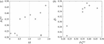
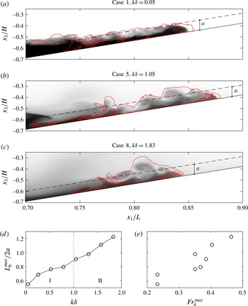
1 Introduction
Breaking internal waves on slopes are of critical oceanographic importance, particularly in quantifying dissipation and mixing in the global ocean energy budget. Munk & Wunsch (Reference Munk and Wunsch1998) suggested that the ocean is primarily mixed by strong turbulent events at boundaries, with the mixed water masses then being exported into the ocean interior. The review of Wunsch & Ferrari (Reference Wunsch and Ferrari2004) expands on this claim by asking whether breaking internal waves at boundaries can account for the global average mixing in the ocean being 10 times higher than the observed open ocean mixing away from topography. A thorough review of breaking internal waves on the continental shelf and slope was made by Lamb (Reference Lamb2014), but the relative contribution of breaking internal waves at boundaries to the global ocean energy budget remains poorly understood.
Shoaling and breaking internal waves on slopes are also important drivers of transport and mixing in nearshore ecosystems. A variety of field observations have quantified the effect of breaking internal waves on the nearshore distributions of biologically important scalars. These include temperature (Leichter et al. Reference Leichter, Wing, Miller and Denny1996; Davis & Monismith Reference Davis and Monismith2011; Walter et al. Reference Walter, Woodson, Arthur, Fringer and Monismith2012), nutrients (Leichter et al. Reference Leichter, Wing, Miller and Denny1996; Omand et al. Reference Omand, Leichter, Franks, Guza, Lucas and Feddersen2011), sediments (Bogucki, Dickey & Redekopp Reference Bogucki, Dickey and Redekopp1997; Klymak & Moum Reference Klymak and Moum2003; Hosegood, Bonnin & van Haren Reference Hosegood, Bonnin and van Haren2004; Hosegood & van Haren Reference Hosegood and van Haren2004; Carter, Gregg & Lien Reference Carter, Gregg and Lien2005; Quaresma et al. Reference Quaresma, Vitorino, Oliveira and da Silva2007), larvae (Pineda Reference Pineda1994) and dissolved oxygen (Walter et al. Reference Walter, Woodson, Leary and Monismith2014b ).
An understanding of the turbulent energetics of stratified flows is necessary to solve the aforementioned oceanographic problems. The turbulent mixing efficiency is particularly important because it allows mixing rates to be inferred from measurements of dissipation. One can use the mixing efficiency to estimate the eddy diffusivity,
 $K_{\unicode[STIX]{x1D70C}}=\unicode[STIX]{x1D6E4}\unicode[STIX]{x1D716}/N^{2}$
, where
 $\unicode[STIX]{x1D6E4}$
is the mixing coefficient,
 $\unicode[STIX]{x1D716}$
is the turbulent dissipation and
 $N$
is the buoyancy frequency (Osborn Reference Osborn1980). Such parameterizations of mixing can also be used in large-scale models that do not resolve small-scale turbulent mixing processes. The mixing efficiency of stratified turbulent flows has traditionally been quantified from the turbulent kinetic energy equation using the flux Richardson number
 $$\begin{eqnarray}R_{f}=\frac{{\mathcal{B}}}{{\mathcal{B}}+\unicode[STIX]{x1D716}},\end{eqnarray}$$
where
 ${\mathcal{B}}$
is the turbulent buoyancy flux (e.g. Osborn Reference Osborn1980; Ivey & Imberger Reference Ivey and Imberger1991; Shih et al.
Reference Shih, Koseff, Ivey and Ferziger2005). The mixing coefficient is related to the flux Richardson number as
 $$\begin{eqnarray}\unicode[STIX]{x1D6E4}=\frac{R_{f}}{1-R_{f}}=\frac{{\mathcal{B}}}{\unicode[STIX]{x1D716}}.\end{eqnarray}$$
Assuming steady, homogeneous turbulence (a balance of turbulent production with the buoyancy flux and dissipation), Osborn (Reference Osborn1980) suggested a critical flux Richardson number
 $R_{f}^{crit}\approx 0.17$
, which gives
 $\unicode[STIX]{x1D6E4}\approx 0.2$
. Based on the relationship between
 $R_{f}$
and
 $\unicode[STIX]{x1D6E4}$
in (1.2), both of these quantities are often referred to as the ‘mixing efficiency’ in the literature. In this paper, we refer to the mixing efficiency as
 $R_{f}$
.
As reviewed by Ivey, Winters & Koseff (Reference Ivey, Winters and Koseff2008), many field studies have examined the mixing efficiency from turbulence measurements in the ocean, finding a range of values for different conditions. These studies use measurements of fine-scale velocity and temperature gradients to quantify the dissipation of turbulent kinetic energy
 $\unicode[STIX]{x1D716}$
and the dissipation of scalar variance
 $\unicode[STIX]{x1D712}$
, respectively. For example, Oakey (Reference Oakey1982) found
 $\unicode[STIX]{x1D6E4}\approx 0.24$
using microstructure profiles of the upper ocean (50–100 m depth), while Yamazaki & Osborn (Reference Yamazaki and Osborn1993) found
 $R_{f}\approx 0.05$
using a submarine-mounted instrument in a turbulent shear layer. Additionally, using microstructure profiles, Seim & Gregg (Reference Seim and Gregg1995) estimated
 $R_{f}=0.22\pm 0.1$
for a shear instability event, Gargett & Moum (Reference Gargett and Moum1995) estimated
 $R_{f}\approx 0.4$
in a turbulent tidal front and Moum (Reference Moum1996) estimated
 $R_{f}=0.13{-}0.17$
in turbulent patches in the main ocean thermocline. Several studies have also inferred how
 $R_{f}$
varies when different parameterizations are used (e.g. Dunckley et al.
Reference Dunckley, Koseff, Steinbuck, Monismith and Genin2012; Bluteau, Jones & Ivey Reference Bluteau, Jones and Ivey2013). The advent of moored turbulence measurements has allowed for the collection of turbulence data over longer time series. Several studies, such as Davis & Monismith (Reference Davis and Monismith2011) and Walter et al. (Reference Walter, Squibb, Woodson, Koseff and Monismith2014a
), have used moored instruments to estimate the mixing efficiency during breaking internal wave events on slopes. While it is clear from these studies that the mixing efficiency depends upon the state of the turbulence that is driving mixing, the intermittent (in time) and patchy (in space) nature of ocean turbulence makes a complete observational understanding of the mixing efficiency difficult.
For this reason, many studies have turned to more idealized laboratory and numerical set-ups to quantify the mixing efficiency of stratified turbulent flows. Using laboratory experiments, Ivey & Imberger (Reference Ivey and Imberger1991) extended the definition of the flux Richardson number to include the entire turbulent kinetic energy budget such that
 $R_{f}={\mathcal{B}}/m$
, where
 $m$
is the net mechanical energy available to sustain turbulent motions (including production, advection and transport). They then characterized
 $R_{f}$
in terms of the turbulent Reynolds number
 $Re_{T}=uL_{C}/\unicode[STIX]{x1D708}$
and the turbulent Froude number
 $Fr_{T}=u/NL_{C}$
, where
 $L_{C}$
is the centred displacement scale, a measure of observed turbulent overturns, and
 $u\sim (\unicode[STIX]{x1D716}L_{C})^{1/3}$
is the turbulent velocity scale. For large enough turbulent Reynolds numbers to sustain turbulence (
 $Re_{T}>15$
), they found that
 $R_{f}$
is maximized for
 $Fr_{T}\approx 1$
. For
 $Fr_{T}<1$
, turbulent mixing is suppressed by buoyancy, while for
 $Fr_{T}>1$
, turbulent mixing is reduced because the stratification is weak. Both Davis & Monismith (Reference Davis and Monismith2011) and Walter et al. (Reference Walter, Squibb, Woodson, Koseff and Monismith2014a
) found good agreement with Ivey & Imberger (Reference Ivey and Imberger1991) using data from field observations of breaking internal waves on slopes, noting the potential effect of the advection of turbulent kinetic energy on the measured mixing efficiency in these events.
Using direct numerical simulations (DNS), Shih et al. (Reference Shih, Koseff, Ivey and Ferziger2005) presented another parameterization of
 $R_{f}$
in terms of the buoyancy Reynolds number or turbulence activity number
 $Re_{b}=\unicode[STIX]{x1D716}/\unicode[STIX]{x1D708}N^{2}$
. They found that for
 $Re_{b}<7$
(the ‘diffusive’ regime),
 $R_{f}$
is scattered and often negative due to countergradient turbulent buoyancy fluxes, ranging from
 $-0.4$
to 0.2. For
 $7<Re_{b}<100$
(the ‘intermediate regime’),
 $R_{f}$
is fairly constant around 0.2, slightly larger than the critical value of Osborn (Reference Osborn1980). For
 $Re_{b}>100$
(the ‘energetic’ regime),
 $R_{f}$
declines as
 $Re_{b}$
increases (
 $R_{f}=\unicode[STIX]{x1D6FC}\,Re_{b}^{-1/2}$
,
 $\unicode[STIX]{x1D6FC}=1.5$
) because the turbulence is actively growing. Several studies have extended the analysis of Shih et al. (Reference Shih, Koseff, Ivey and Ferziger2005) to larger values of
 $Re_{b}$
, which are common in the field but infeasible in DNS. Both Davis & Monismith (Reference Davis and Monismith2011) and Walter et al. (Reference Walter, Squibb, Woodson, Koseff and Monismith2014a
) found a similar power-law relationship between
 $R_{f}$
and
 $Re_{b}$
in the energetic regime, with
 $\unicode[STIX]{x1D6FC}=4.5$
and
 $\unicode[STIX]{x1D6FC}=2$
, respectively. A direct comparison between the results of Shih et al. (Reference Shih, Koseff, Ivey and Ferziger2005), Davis & Monismith (Reference Davis and Monismith2011) and Walter et al. (Reference Walter, Squibb, Woodson, Koseff and Monismith2014a
) is presented in Walter et al. (Reference Walter, Squibb, Woodson, Koseff and Monismith2014a
), see figure 12 therein. It should be noted that the coefficient
 $\unicode[STIX]{x1D6FC}$
is not universally
 $O(1)$
. A study of stratified turbulence in the atmospheric boundary layer by Lozovatsky & Fernando (Reference Lozovatsky and Fernando2013) again found
 $R_{f}=\unicode[STIX]{x1D6FC}Re_{b}^{-1/2}$
scaling, but with
 $\unicode[STIX]{x1D6FC}=50$
. Mater & Venayagamoorthy (Reference Mater and Venayagamoorthy2014) have since reconsidered the results of Shih et al. (Reference Shih, Koseff, Ivey and Ferziger2005) in terms of a shear strength parameter
 $ST_{L}=Sk/\unicode[STIX]{x1D716}$
, a turbulent Froude number
 $Fr_{k}=\unicode[STIX]{x1D716}/Nk$
and a turbulent Reynolds number
 $Re_{L}=k^{2}/\unicode[STIX]{x1D708}\unicode[STIX]{x1D716}$
, where
 $S$
is the mean shear and
 $k$
is the turbulent kinetic energy. Using this framework, they discussed the potential ambiguities of using single parameters such as
 $Re_{b}$
and the gradient Richardson number
 $Ri_{g}=N^{2}/S^{2}$
to characterize the mixing efficiency.
The mixing efficiency of stratified turbulent flows can also be quantified by separating the potential energy into its available and background components (Winters et al.
Reference Winters, Lombard, Riley and D’Asaro1995). The background potential energy represents the lowest possible potential energy state of a system if it were to be adiabatically rearranged, and is obtained numerically by sorting the density field. The available potential energy, then, is the difference between the total potential energy and the background, and is available for exchange with the kinetic energy. Changes in the background potential energy can only occur due to molecular diffusion, and therefore represent a true measure of irreversible mixing. Reversible turbulent ‘stirring’ is contained in the available potential energy field. Winters et al. (Reference Winters, Lombard, Riley and D’Asaro1995) used these definitions to define a volume-integrated measure of the mixing efficiency. Several studies have employed this method to quantify the energetics of stratified shear flows. Smyth, Moum & Caldwell (Reference Smyth, Moum and Caldwell2001) used DNS to compare mixing efficiency values calculated with the Winters et al. (Reference Winters, Lombard, Riley and D’Asaro1995) method to a typical approximation used in the field, the Osborn–Cox model (Osborn & Cox Reference Osborn and Cox1972), which is based on the dissipation of scalar variance
 $\unicode[STIX]{x1D712}$
. Peltier & Caulfield (Reference Peltier and Caulfield2003) also used the Winters et al. (Reference Winters, Lombard, Riley and D’Asaro1995) method to relate a cumulative measure of the mixing efficiency to the initial Richardson number
 $Ri_{0}$
.
Much of the laboratory and numerical work examining the mixing efficiency of stratified turbulent flows has focused directly on breaking internal wave events. For example, Michallet & Ivey (Reference Michallet and Ivey1999) and Boegman, Ivey & Imberger (Reference Boegman, Ivey and Imberger2005) calculated the bulk mixing efficiency of breaking internal wave events on a slope in the laboratory, finding a range of mixing efficiency values between 0.05 and 0.25 for various wave and slope conditions. Their mixing efficiency calculation was based on the total potential energy gain in the system due to the breaking wave event. Additionally, Hult, Troy & Koseff (Reference Hult, Troy and Koseff2011) calculated the mixing efficiency within turbulent patches generated by breaking internal waves propagating over a ridge. However, due to the difficulty of measuring the turbulent buoyancy flux
 ${\mathcal{B}}$
in the laboratory, they calculated dissipation and inferred
 $R_{f}$
from the parameterizations of Ivey & Imberger (Reference Ivey and Imberger1991) and Shih et al. (Reference Shih, Koseff, Ivey and Ferziger2005), and found
 $R_{f}\approx 0.10-0.17$
in the turbulent patch created by wave breaking. Although turbulence existed in the upper and lower density layers during their experiments, it did not contribute to mixing because these layers were unstratified (thus
 $R_{f}\approx 0$
there). This resulted in an overall
 $R_{f}$
of 0.04–0.07 for the entire domain.
Using numerical simulations, Fringer & Street (Reference Fringer and Street2003) employed the method of Winters et al. (Reference Winters, Lombard, Riley and D’Asaro1995) to calculate the mixing efficiency of breaking progressive internal waves as a function of the non-dimensional pycnocline thickness
 $k\unicode[STIX]{x1D6FF}$
. They found an average bulk mixing efficiency of 0.42, with a peak around 0.49 when
 $k\unicode[STIX]{x1D6FF}\approx 1$
. This corresponds to the most efficient transfer of energy from the large-scale wave to the turbulent scales, where mixing takes place. Finally, Arthur & Fringer (Reference Arthur and Fringer2014) used the method of Winters et al. (Reference Winters, Lombard, Riley and D’Asaro1995) to quantify the energetics of breaking internal waves on slopes. They calculated the bulk mixing efficiency as a function of the incoming wave amplitude and bathymetric slope, and found a range of values between 0.14 and 0.20.
There are several drawbacks associated with the mixing efficiency measures explained above. First, the flux Richardson number
 $R_{f}$
is affected by countergradient turbulent buoyancy fluxes, especially at low Reynolds number
 $Re_{b}$
, leading to small and potentially negative values of
 $R_{f}$
(Venayagamoorthy & Koseff Reference Venayagamoorthy and Koseff2016). Second, the Winters et al. (Reference Winters, Lombard, Riley and D’Asaro1995) method relies on domain-integrated quantities of dissipation and mixing in order to define the mixing efficiency. Thus, the energetics cannot be broken down into smaller (local) regions of the flow. In order to address both of these issues, Scotti & White (Reference Scotti and White2014) developed a new measure of local turbulent energetics based on a local definition of the rate of change of the background potential energy. Their method builds upon the framework of Winters et al. (Reference Winters, Lombard, Riley and D’Asaro1995) to provide a measure of irreversible turbulent mixing. This facilitates calculations of local turbulent mixing efficiency that are not affected by countergradient buoyancy fluxes. The method of Scotti & White (Reference Scotti and White2014) has yet to be applied to the problem of breaking internal waves on slopes.
In the present study, we use the method of Scotti & White (Reference Scotti and White2014) to explore local and volume-integrated measures of turbulence and mixing in breaking internal waves on slopes. We focus on the effect of pycnocline thickness on turbulence and mixing, which is relevant in lakes and the coastal ocean, but has not been considered in previous laboratory-scale studies of breaking internal waves on slopes (e.g. Michallet & Ivey Reference Michallet and Ivey1999; Boegman et al. Reference Boegman, Ivey and Imberger2005; Arthur & Fringer Reference Arthur and Fringer2014). We employ DNS to consider eight breaking wave cases with a range of pycnocline thicknesses, but with fixed initial amplitude, and therefore similar incoming wave properties. Section 2 explains our computational approach, which is based on that of Arthur & Fringer (Reference Arthur and Fringer2014) and Arthur & Fringer (Reference Arthur and Fringer2016). Section 3 provides an overview of the breaking process for different pycnocline thicknesses. Then, in §§ 4 and 5, we explore local and volume-integrated turbulent energetics quantities, respectively. Finally, in § 6, we present a connection between local and volume-integrated energetics perspectives.
2 Computational approach
2.1 Computational set-up
We perform DNS of breaking internal waves on slopes in an idealized, laboratory-scale domain using the parallel Navier–Stokes code of Cui (Reference Cui1999). This code employs the fractional-step method of Zang, Street & Koseff (Reference Zang, Street and Koseff1994), and has been used extensively in the past to study geophysical flows at the laboratory scale (see Venayagamoorthy & Fringer Reference Venayagamoorthy and Fringer2007; Chou & Fringer Reference Chou and Fringer2010; Arthur & Fringer Reference Arthur and Fringer2014, Reference Arthur and Fringer2016). The computational set-up used here is based on that of Arthur & Fringer (Reference Arthur and Fringer2014, Reference Arthur and Fringer2016), and is summarized in figure 1.
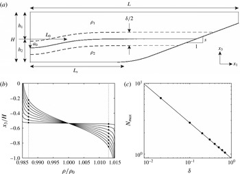
The computational set-up used to study breaking internal waves on slopes. (
 $x_{1}$
,
 $x_{2}$
,
 $x_{3}$
) are Cartesian coordinates in the cross-shore, lateral (along shore, into the page) and vertical directions, respectively. (a) A schematic of the domain, where the length
 $L=4~\text{m}$
, the total depth
 $H=0.56~\text{m}$
, the upper-layer depth
 $h_{1}=0.3~\text{m}$
, the lower-layer depth
 $h_{2}=0.26~\text{m}$
, the upper-layer density
 $\unicode[STIX]{x1D70C}_{1}=985~\text{kg}~\text{m}^{-3}$
, the lower-layer density
 $\unicode[STIX]{x1D70C}_{2}=1015~\text{kg}~\text{m}^{-3}$
, the slope
 $s=0.218$
, the amplitude of the initial half-Gaussian
 $a_{0}=0.1~\text{m}$
and the length scale of the initial half-Gaussian
 $L_{0}=0.7~\text{m}$
. The length of the flat region before the slope begins is
 $L_{s}=1.675~\text{m}$
and the radius of curvature of the rounded bottom at the beginning of the slope is 3 m. The pycnocline thickness
 $\unicode[STIX]{x1D6FF}$
varies for each case and is shown in table 1. The lateral (
 $x_{2}$
, into the page) width of the domain is
 $W=0.1$
m. (b) The initial density profile for each case, as defined in (2.1). The stratified region around the interface
 $x_{3}=-h_{1}\pm \unicode[STIX]{x1D6FF}/4$
is highlighted by the intersection of the vertical dotted lines at
 $\unicode[STIX]{x1D70C}/\unicode[STIX]{x1D70C}_{0}=0.987,1.013$
with each density profile. (c) The maximum buoyancy frequency for each case
 $N_{max}$
as a function of
 $\unicode[STIX]{x1D6FF}$
, including a scaling line of
 $N_{max}\sim \unicode[STIX]{x1D6FF}^{-1/2}$
(Troy & Koseff Reference Troy and Koseff2005).

Computations are made on an orthogonal curvilinear grid of size
 $n_{1}\times n_{2}\times n_{3}=1152\times 96\times 128\approx 14\times 10^{6}$
points that was generated using the open-source software gridgen (available online at https://code.google.com/p/gridgen-c/). Grid stretching of the form
 $\unicode[STIX]{x0394}x_{i}^{k}=r\unicode[STIX]{x0394}x_{i}^{k+1}$
, where
 $r$
is the stretching factor and
 $k$
is the index of the grid point, is employed in the horizontal (
 $x_{1}$
) and vertical (
 $x_{3}$
) directions to increase resolution in the breaking region. Grid spacing in the lateral (
 $x_{2}$
) direction is constant. In the horizontal direction, stretching is applied from
 $x_{1}=0$
to
 $L_{s}$
with
 $r=1.01$
, concentrating 1024 points (approximately 90 % of
 $n_{1}$
) into the sloping region. The grid is also stretched slightly in
 $x_{1}$
in the sloping region to maintain orthogonality. In the vertical direction, stretching is performed twice. First, grid points are concentrated toward the bottom with
 $r=1.02$
in order to resolve the flow near the wall. Second, 100 of 128 points (78 %) are concentrated in the bottom 35 % of the domain with
 $r=1.07$
in order to resolve the pycnocline and lower layer during breaking. The resulting grid resolution at the pycnocline in the breaking region is approximately
 $\unicode[STIX]{x0394}x_{1}\times \unicode[STIX]{x0394}x_{2}\times \unicode[STIX]{x0394}x_{3}=4~\text{mm}\times 1~\text{mm}\times 2~\text{mm}$
. Near the bottom wall, the vertical coordinate is measured in wall units
 $x_{3}^{+}=x_{3}/\unicode[STIX]{x1D6FF}_{S}$
, where
 $\unicode[STIX]{x1D6FF}_{S}=\sqrt{2\unicode[STIX]{x1D708}/\unicode[STIX]{x1D714}}$
(see § 2.2 for the definition of the wave frequency
 $\unicode[STIX]{x1D714}$
). The vertical resolution near the wall is therefore
 $\unicode[STIX]{x0394}x_{3}^{+}=\unicode[STIX]{x0394}x_{3}/\unicode[STIX]{x1D6FF}_{S}<1$
. In the worst case scenario, the grid spacing is found to be within approximately one order of magnitude of the Kolmogorov length scale
 $\unicode[STIX]{x1D702}_{k}$
, providing sufficient resolution for DNS (see Arthur & Fringer Reference Arthur and Fringer2014). The boundary conditions for all velocity components are no slip on the bottom wall and free slip on the top, left and right walls. The density field has a gradient-free boundary condition on the top, bottom, left and right walls. All variables are periodic in the lateral (
 $x_{2}$
) direction.
A time step of
 $\unicode[STIX]{x0394}t=0.003$
s is used for all simulations. The number of time steps varies by case and ranges from 18 000 for case 1 to for 27 000 for case 8. Simulations were run on the US Army Research Lab Department of Defense Supercomputing Research Center (ARL DSRC) supercomputer Pershing using 432 processors. With a computation time of approximately 20 s per time step, this resulted in wall-clock simulation times ranging from 100 h (43 000 processor h; case 1) to 150 h (65 000 processor h; case 8).
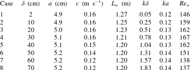
The breaking wave cases considered in this study in terms of the pycnocline thickness
 $\unicode[STIX]{x1D6FF}$
, the wave amplitude
 $a$
, the wave speed
 $c$
and the wave length scale
 $L_{w}$
, the normalized interface thickness
 $k\unicode[STIX]{x1D6FF}$
, the wave steepness
 $ka$
and the wave Reynolds number
 $Re_{w}$
.

2.2 Initial wave parameters
We consider eight breaking wave cases with varying pycnocline thickness
 $\unicode[STIX]{x1D6FF}$
, as summarized in table 1. The stratification within the domain is initialized as
 $$\begin{eqnarray}\frac{\unicode[STIX]{x1D70C}}{\unicode[STIX]{x1D70C}_{0}}(x_{1},x_{3},\unicode[STIX]{x1D70F}=0)=1-\frac{\unicode[STIX]{x0394}\unicode[STIX]{x1D70C}}{2\unicode[STIX]{x1D70C}_{0}}\tanh \bigg[\frac{2(x_{3}+h_{1}+\unicode[STIX]{x1D701}(x_{1}))}{\unicode[STIX]{x1D6FF}}\tanh ^{-1}(\unicode[STIX]{x1D6FC})\bigg],\end{eqnarray}$$
where the reference density
 $\unicode[STIX]{x1D70C}_{0}=1000~\text{kg}~\text{m}^{-3}$
, the density difference between the top and bottom layers is
 $\unicode[STIX]{x0394}\unicode[STIX]{x1D70C}=\unicode[STIX]{x1D70C}_{2}-\unicode[STIX]{x1D70C}_{1}=30~\text{kg}~\text{m}^{-3}$
, the upper-layer depth
 $h_{1}=0.3$
m, and
 $\unicode[STIX]{x1D6FC}=0.99$
. The pycnocline thickness
 $\unicode[STIX]{x1D6FF}$
determines the buoyancy frequency
 $N=\sqrt{-(g/\unicode[STIX]{x1D70C}_{0})\unicode[STIX]{x2202}\unicode[STIX]{x1D70C}/\unicode[STIX]{x2202}x_{3}}$
of the initial stratification; the maximum buoyancy frequency
 $N_{max}$
scales with
 $\unicode[STIX]{x1D6FF}^{-1/2}$
(Troy & Koseff Reference Troy and Koseff2005), as is shown for each case in figure 1(c). Throughout the paper, we refer to time using the variable
 $\unicode[STIX]{x1D70F}$
in order to avoid confusion with
 $t$
, which stands for ‘turbulent’ in the notation of Scotti & White (Reference Scotti and White2014).
A wave of depression is created in the domain by initializing a half-Gaussian at the left boundary. The shape of the interface is given by
 $$\begin{eqnarray}\unicode[STIX]{x1D701}(x_{1})=a_{0}\exp \left[-\left(\frac{x_{1}}{L_{0}}\right)^{2}\right]+\unicode[STIX]{x1D701}^{\prime }R,\end{eqnarray}$$
where
 $a_{0}=0.1~\text{m}$
and
 $L_{0}=0.7~\text{m}$
are the initial amplitude and length scale of the half-Gaussian, respectively. An initial perturbation
 $\unicode[STIX]{x1D701}^{\prime }R$
, where
 $\unicode[STIX]{x1D701}^{\prime }=1~\text{mm}$
and
 $R\in \{-1,1\}$
is a uniformly distributed random number, is also added to the interface to trigger lateral instabilities during breaking. Relaxation of the initial half-Gaussian produces an internal wave of depression that propagates toward the slope and breaks. We note that the initial wave is solitary-like, but that it does not necessarily satisfy the Dubreil–Jacotin–Long (DJL) equation for internal solitary waves (see Lamb Reference Lamb2002, and references therein). We therefore refer to the waves in this study more generally as ‘internal waves’. Further discussion of the difference between the waves in the present study and true DJL internal solitary waves can be found in Arthur & Fringer (Reference Arthur and Fringer2016).
Here, case 1 corresponds to case 3 from Arthur & Fringer (Reference Arthur and Fringer2014) and cases 3t1/3t2 from Arthur & Fringer (Reference Arthur and Fringer2016). The additional cases 2–8 differ from this ‘base case’ only in the value of
 $\unicode[STIX]{x1D6FF}$
; all other initial parameters are held constant. As a result of changing
 $\unicode[STIX]{x1D6FF}$
, the other properties of the incoming wave (after it has formed from the initial half-Gaussian) change slightly relative to the base case (see table 1). These properties, including the wave amplitude
 $a$
, the wave speed
 $c$
and the wave length scale
 $L_{w}=1/a\int _{0}^{L_{s}}\unicode[STIX]{x1D702}(x_{1})\,\text{d}x_{1}$
, where
 $\unicode[STIX]{x1D702}$
is the displacement of the
 $\unicode[STIX]{x1D70C}=\unicode[STIX]{x1D70C}_{0}$
isopycnal from
 $x_{3}=-h_{1}$
(Michallet & Ivey Reference Michallet and Ivey1999), are calculated after the wave has formed but before it begins to interact with the slope.
In order to quantify the effect of changing the pycnocline thickness
 $\unicode[STIX]{x1D6FF}$
on the incoming wave, we classify each breaking wave case in terms of the relevant non-dimensional parameters, including
 $k\unicode[STIX]{x1D6FF}$
,
 $ka$
and
 $Re_{w}$
(Troy & Koseff Reference Troy and Koseff2005), as shown in table 1:
 $k\unicode[STIX]{x1D6FF}$
is the normalized pycnocline thickness, where the horizontal wavenumber
 $k=2\unicode[STIX]{x03C0}/\unicode[STIX]{x1D706}$
and
 $\unicode[STIX]{x1D706}\approx 2L_{w}$
;
 $ka$
is the wave steepness;
 $Re_{w}=a^{2}\unicode[STIX]{x1D714}/\unicode[STIX]{x1D708}$
is the wave Reynolds number, where the wave frequency
 $\unicode[STIX]{x1D714}=c/\unicode[STIX]{x1D706}$
. We note that the value of
 $Re_{w}=146$
reported here for case 1 differs from the value of
 $Re_{w}=208$
reported for the same case in Arthur & Fringer (Reference Arthur and Fringer2014) and Arthur & Fringer (Reference Arthur and Fringer2016). Here, we use the actual wave speed
 $c$
as opposed to the linear phase speed in a two-layer system that was used previously. As shown in table 1, the normalized pycnocline thickness varies by nearly two orders of magnitude from case 1 to case 8. However,
 $ka$
and
 $Re_{w}$
change by no more than 20 % from the base case. The bathymetric slope
 $s$
is also held constant. We therefore focus our analysis on how the energetics of wave breaking change with the normalized pycnocline thickness
 $k\unicode[STIX]{x1D6FF}$
. Troy & Koseff (Reference Troy and Koseff2005) considered the combined effect of the pycnocline thickness
 $k\unicode[STIX]{x1D6FF}$
and the wave steepness
 $ka$
using the wave Richardson number
 $Ri_{w}\sim k\unicode[STIX]{x1D6FF}/(ka)^{2}$
. However, we do not consider
 $Ri_{w}$
here because
 $ka$
is roughly constant and therefore
 $Ri_{w}\sim k\unicode[STIX]{x1D6FF}$
.
3 General description of wave breaking
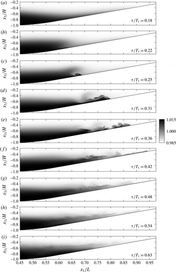
The density structure over the course of the breaking event is similar for each case, and is shown in figure 2 for case 5 (
 $k\unicode[STIX]{x1D6FF}\approx 1$
). In this figure and others, we present the time
 $\unicode[STIX]{x1D70F}$
normalized by the wave period for case 1,
 $T_{1}=2\unicode[STIX]{x03C0}/\unicode[STIX]{x1D714}_{1}$
. As the wave begins to interact with the slope, downslope flow is concentrated in the lower layer beneath the leading face (figure 2
a). At the same time, the rear face steepens (figure 2
b). The downslope flow beneath the leading face and the upslope flow beneath the rear face then interact to create the shear that initializes the breaking event (figure 2
c).
Snapshots in time of the density structure
 $\unicode[STIX]{x1D70C}/\unicode[STIX]{x1D70C}_{0}$
for breaking wave case 5 (
 $k\unicode[STIX]{x1D6FF}\approx 1$
). Results are averaged in the lateral (
 $x_{2}$
) direction. The time shown in (c) represents the breakpoint, shown in figure 5(e), while the time shown in (e) represents the time of maximum turbulent mixing
 $(\unicode[STIX]{x1D716}_{p}^{t})_{max}^{V}$
(5.2), shown in figures 4 and 5(m).

After breaking, a surge of dense fluid flows up the slope, creating shear instabilities (billows) at the interface (figure 2
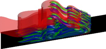
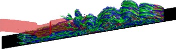
d,e). These billows create regions of unstable stratification that are subject to secondary convective instability. A region of unstable stratification is also created under the nose of the upslope surge, leading to the lobe and cleft instability typical of gravity currents (Simpson Reference Simpson1972; Härtel, Carlsson & Thunblom Reference Härtel, Carlsson and Thunblom2000). Figure 3 shows the development of lateral instabilities in these two regions after breaking for case 5. A three-dimensional view of the upslope surge that depicts the fully turbulent flow field for case 5 is shown in figure 4. After the upslope surge reaches its maximum onshore position (figure 2
f), dense fluid flows back downslope (figure 2
g–i) and the pycnocline returns to approximately its initial horizontal position (figure 2
i). As in Arthur & Fringer (Reference Arthur and Fringer2014, Reference Arthur and Fringer2016), we define the end of the breaking event
 $\unicode[STIX]{x1D70F}_{f}$
as the time just before dissipation begins to rise due to a second upslope surge of dense fluid (see figure 9
a). This second upslope surge arises from small waves trailing behind the initial wave due to the initial condition, but is not considered in our results.
All of the breaking waves in this study can be classified as ‘collapsing breakers’ (Boegman et al.
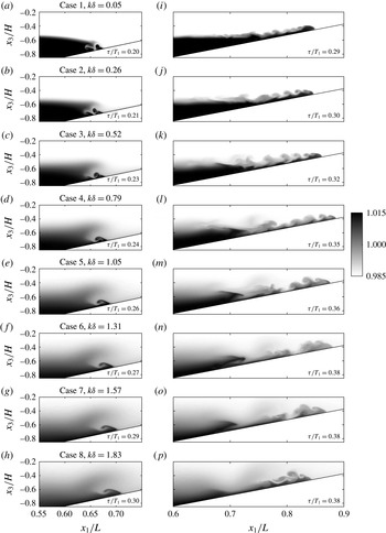
Reference Boegman, Ivey and Imberger2005; Aghsaee, Boegman & Lamb Reference Aghsaee, Boegman and Lamb2010; Arthur & Fringer Reference Arthur and Fringer2014) or ‘backward overturning’ (Moore, Koseff & Hult Reference Moore, Koseff and Hult2016) since the steepening rear face is swept (collapses) backward before it is able to plunge forward. However, several differences can be seen in the breaking event among cases 1–8. The first occurs just before the backward collapse, as a tongue of dense water is forced into the interior of the water column by the upslope momentum of the wave. This dense tongue becomes larger as
 $k\unicode[STIX]{x1D6FF}$
increases (see figure 5
a–h). Additionally, during the upslope surge (figure 5
i–p), the vertical length scale of the billows at the interface changes with
 $k\unicode[STIX]{x1D6FF}$
. Specifically, as
 $k\unicode[STIX]{x1D6FF}$
increases, the billows appear larger relative to the height of the upslope surge. The effects of this change in scale will be discussed further in § 6.
A three-dimensional view of lateral instabilities developing after breaking for case 5 (
 $k\unicode[STIX]{x1D6FF}\approx 1$
), corresponding to figure 2(d). Isosurfaces of
 $\unicode[STIX]{x1D70C}=\unicode[STIX]{x1D70C}_{0}$
(red),
 $\unicode[STIX]{x1D6FA}_{1}/\unicode[STIX]{x1D714}_{1}=24$
(blue) and
 $\unicode[STIX]{x1D6FA}_{1}/\unicode[STIX]{x1D714}_{1}=-24$
(green) are shown.
 $\unicode[STIX]{x1D6FA}_{1}$
is the longitudinal vorticity, representing the ‘streamwise rolls’ discussed in Arthur & Fringer (Reference Arthur and Fringer2014).

A three-dimensional view of the turbulent flow field during the upslope surge for case 5 (
 $k\unicode[STIX]{x1D6FF}\approx 1$
), corresponding to figures 2(e) and 5(m). Isosurfaces of
 $\unicode[STIX]{x1D70C}=\unicode[STIX]{x1D70C}_{0}$
(red),
 $\unicode[STIX]{x1D6FA}_{1}/\unicode[STIX]{x1D714}_{1}=37$
(blue) and
 $\unicode[STIX]{x1D6FA}_{1}/\unicode[STIX]{x1D714}_{1}=-37$
(green) are shown.

Snapshots of the density structure
 $\unicode[STIX]{x1D70C}/\unicode[STIX]{x1D70C}_{0}$
for breaking wave cases 1–8. Results are averaged in the lateral (
 $x_{2}$
) direction. Column (a–h) depicts the wave at the time of breaking, while column (i–p) shows the upslope surge of dense fluid after breaking at the time of maximum turbulent mixing
 $(\unicode[STIX]{x1D716}_{p}^{t})_{max}^{V}$
(5.2).

4 Local turbulent energetics
4.1 Local definitions of turbulent dissipation, mixing and mixing efficiency
The local mixing efficiency of stratified turbulent flows has traditionally been quantified using the flux Richardson number
 $R_{f}={\mathcal{B}}/({\mathcal{B}}+\unicode[STIX]{x1D716})$
(1.1), where
 ${\mathcal{B}}=(g/\unicode[STIX]{x1D70C}_{0})\overline{\unicode[STIX]{x1D70C}^{\prime }u_{3}^{\prime }}$
is the turbulent buoyancy flux and
 $\unicode[STIX]{x1D716}=2\unicode[STIX]{x1D708}\overline{\unicode[STIX]{x1D61A}_{ij}^{\prime }\unicode[STIX]{x1D61A}_{ij}^{\prime }}$
is the turbulent dissipation (e.g. Osborn Reference Osborn1980; Ivey & Imberger Reference Ivey and Imberger1991; Shih et al.
Reference Shih, Koseff, Ivey and Ferziger2005). The turbulent rate of strain tensor is
 $\unicode[STIX]{x1D61A}_{ij}^{\prime }=((\unicode[STIX]{x2202}u_{i}^{\prime }/\unicode[STIX]{x2202}x_{j})+(\unicode[STIX]{x2202}u_{j}^{\prime }/\unicode[STIX]{x2202}x_{i}))/2$
. The overbar denotes a Reynolds average, while the prime denotes a departure from that average. As discussed by Venayagamoorthy & Koseff (Reference Venayagamoorthy and Koseff2016), the turbulent buoyancy flux
 ${\mathcal{B}}$
can include reversible countergradient fluxes, leading to low or negative values of
 $R_{f}$
, especially in weakly turbulent conditions. Interpretation of
 $R_{f}$
using this method is further complicated in the presence of unsteady, inhomogeneous turbulence due to the difficulty in choosing the appropriate Reynolds average (e.g. Hult et al.
Reference Hult, Troy and Koseff2011). Thus, even in the current DNS study, it is difficult to interpret the meaning of
 $R_{f}$
.
To address the problems associated with quantifying turbulent dissipation, mixing and mixing efficiency in regions of unsteady, inhomogeneous turbulence, Scotti & White (Reference Scotti and White2014) developed a new method of analysis based on a locally defined background potential energy. Their method builds upon the background potential energy framework of Winters et al. (Reference Winters, Lombard, Riley and D’Asaro1995) to define local turbulent dissipation and irreversible turbulent mixing quantities. Turbulent dissipation is defined as above,
 $$\begin{eqnarray}\unicode[STIX]{x1D716}_{k}^{t}=2\unicode[STIX]{x1D708}\overline{\unicode[STIX]{x1D61A}_{ij}^{\prime }\unicode[STIX]{x1D61A}_{ij}^{\prime }},\end{eqnarray}$$
where we have adopted the notation of Scotti & White (Reference Scotti and White2014) for clarity. Irreversible turbulent mixing is defined as the turbulent dissipation of available potential energy,
 $$\begin{eqnarray}\unicode[STIX]{x1D716}_{p}^{t}=\unicode[STIX]{x1D705}\left(\frac{\overline{|\unicode[STIX]{x1D6FB}b|^{2}}}{N_{\ast }^{2}(b)}-\frac{|\unicode[STIX]{x1D6FB}\overline{b}|^{2}}{N_{\ast }^{2}(\overline{b})}\right)\simeq \unicode[STIX]{x1D705}\frac{\overline{|\unicode[STIX]{x1D6FB}b^{\prime }|^{2}}}{N_{\ast }^{2}(\overline{b})},\end{eqnarray}$$
where
 $b(x_{1},x_{2},x_{3},\unicode[STIX]{x1D70F})=g(\unicode[STIX]{x1D70C}-\unicode[STIX]{x1D70C}_{0})/\unicode[STIX]{x1D70C}_{0}$
is the buoyancy field and
 $N_{\ast }^{2}(x_{3},\unicode[STIX]{x1D70F})$
is the squared buoyancy frequency of the background density field
 $\unicode[STIX]{x1D70C}_{\ast }(x_{3},\unicode[STIX]{x1D70F})$
. The background density field represents the lowest possible potential energy state of the system if it were to be adiabatically rearranged (Winters et al.
Reference Winters, Lombard, Riley and D’Asaro1995), and is obtained numerically by sorting the density field
 $\unicode[STIX]{x1D70C}$
. Changes in the background potential energy can only occur due to molecular diffusion, and are therefore irreversible. In the present study, the Reynolds average overbar denotes a lateral average (in the
 $x_{2}$
direction), while the prime denotes a departure from that average. Our calculations of
 $\unicode[STIX]{x1D716}_{k}^{t}$
and
 $\unicode[STIX]{x1D716}_{p}^{t}$
are therefore functions of
 $x_{1}$
,
 $x_{3}$
and
 $\unicode[STIX]{x1D70F}$
. In (4.2),
 $N_{\ast }^{2}(b)$
is found by mapping the given local value of
 $b$
to a corresponding value of
 $N_{\ast }^{2}$
in the background buoyancy frequency profile and is therefore a function of
 $x_{1}$
,
 $x_{2}$
,
 $x_{3}$
and
 $\unicode[STIX]{x1D70F}$
. Alternatively,
 $N_{\ast }^{2}(\overline{b})$
must be found by interpolating
 $N_{\ast }^{2}$
to the given value of
 $\overline{b}$
, and is therefore a function of
 $x_{1}$
,
 $x_{3}$
and
 $\unicode[STIX]{x1D70F}$
.
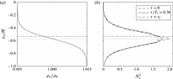
(a) The background density field
 $\unicode[STIX]{x1D70C}_{\ast }/\unicode[STIX]{x1D70C}_{0}$
and (b) the background buoyancy frequency field
 $N_{\ast }^{2}$
used in the calculation of
 $\unicode[STIX]{x1D716}_{p}^{t}$
. Data are shown for case 5 (
 $k\unicode[STIX]{x1D6FF}\approx 1$
) at the time of maximum turbulent mixing
 $(\unicode[STIX]{x1D716}_{p}^{t})_{max}^{V}$
(5.2), which corresponds to the time shown in figures 2(e), 4 and 5(m). The background buoyancy frequency is shown at
 $\unicode[STIX]{x1D70F}=0$
and
 $\unicode[STIX]{x1D70F}=\unicode[STIX]{x1D70F}_{f}$
in (b) as well. The horizontal dotted line denotes the vertical location of the maximum background buoyancy frequency
 $N_{\ast }^{2}$
at
 $\unicode[STIX]{x1D70F}/T_{1}=0.36$
, while the horizontal dash-dot line denotes the vertical location of the initial pycnocline
 $x_{3}=-h_{1}$
.

Irreversible mixing leads to a decrease in the maximum background buoyancy frequency over time. This is shown in figure 6, which presents example calculations of the background density field
 $\unicode[STIX]{x1D70C}_{\ast }$
and background buoyancy frequency field
 $N_{\ast }^{2}$
for case 5. The background buoyancy frequency is shown for the initial condition
 $\unicode[STIX]{x1D70F}=0$
, during the upslope surge at
 $\unicode[STIX]{x1D70F}/T_{1}=0.36$
(the time shown in figures 2
e, 4 and 5
m), and at the end of the breaking event
 $\unicode[STIX]{x1D70F}=\unicode[STIX]{x1D70F}_{f}$
. The background density field is only shown for the intermediate time
 $\unicode[STIX]{x1D70F}/T_{1}=0.36$
because the change from
 $\unicode[STIX]{x1D70F}=0$
to
 $\unicode[STIX]{x1D70F}=\unicode[STIX]{x1D70F}_{f}$
is not discernible in the figure. The horizontal dotted line denotes the vertical location of the maximum buoyancy frequency at
 $\unicode[STIX]{x1D70F}/T_{1}=0.36$
, which is slightly below
 $x_{3}=-h_{1}$
because there is initially less lower-layer fluid (
 $\unicode[STIX]{x1D70C}=\unicode[STIX]{x1D70C}_{2}$
) than upper-layer fluid (
 $\unicode[STIX]{x1D70C}=\unicode[STIX]{x1D70C}_{1}$
) in the domain due to the sloping bottom. Layering is also evident in the background density field (figure 6
a), along with the corresponding wiggles in
 $N_{\ast }^{2}$
(figure 6
b).
Using the definitions of turbulent dissipation and irreversible turbulent mixing in (4.1) and (4.2) above, the local irreversible flux Richardson number can be calculated with
 $$\begin{eqnarray}R_{f}^{\ast }=\frac{\unicode[STIX]{x1D716}_{p}^{t}}{\unicode[STIX]{x1D716}_{p}^{t}+\unicode[STIX]{x1D716}_{k}^{t}}.\end{eqnarray}$$
This measure of the flux Richardson number is not affected by countergradient buoyancy fluxes, and is therefore a preferable measure of the local mixing efficiency to
 $R_{f}$
(Scotti & White Reference Scotti and White2014; Venayagamoorthy & Koseff Reference Venayagamoorthy and Koseff2016).
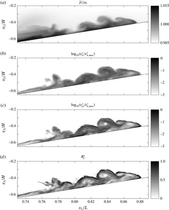
Example local turbulent energetics calculations for case 5 (
 $k\unicode[STIX]{x1D6FF}\approx 1$
) at the time of maximum turbulent mixing
 $(\unicode[STIX]{x1D716}_{p}^{t})_{max}^{V}$
((5.2), corresponding to the time shown in figures 2(e), 4 and 5(m)). Shown are (a) the density field
 $\overline{\unicode[STIX]{x1D70C}}/\unicode[STIX]{x1D70C}_{0}$
, (b) the turbulent dissipation
 $\unicode[STIX]{x1D716}_{k}^{t}$
, (c) the turbulent mixing
 $\unicode[STIX]{x1D716}_{p}^{t}$
, and (d) the local irreversible flux Richardson number
 $R_{f}^{\ast }$
. In (b) and (c), the turbulent quantities are normalized by the maximum turbulent dissipation at the time shown,
 $\unicode[STIX]{x1D716}_{k,max}^{t}$
. Note that in (d), the
 $R_{f}^{\ast }$
field is restricted to locations where
 $Re_{L}>10$
for clarity (
 $Re_{L}$
is defined in (4.7)), while (a), (b) and (c) include the full field.

Local turbulent dissipation and irreversible mixing quantities are calculated over time for each breaking wave case. For illustrative purposes, we consider these quantities for case 5 during the upslope surge of dense fluid after breaking, when shear instabilities (billows) are present at the interface (figure 7
a). At this time, turbulent dissipation
 $\unicode[STIX]{x1D716}_{k}^{t}$
and mixing
 $\unicode[STIX]{x1D716}_{p}^{t}$
are elevated throughout the upslope surge (figure 7
b,c). However, mixing is more concentrated along the roll-up regions of the billows and the nose of the upslope surge (figure 7
c), where sharp density gradients are present. A similar result was noted by Smyth et al. (Reference Smyth, Moum and Caldwell2001), who used the dissipation rate of scalar variance
 $\unicode[STIX]{x1D712}=2\unicode[STIX]{x1D705}\overline{|\unicode[STIX]{x1D6FB}\unicode[STIX]{x1D70C}^{\prime }|^{2}}$
to examine turbulent mixing during the breakdown of Kelvin–Helmholtz billows. The quantity
 $\unicode[STIX]{x1D712}$
is related to
 $\unicode[STIX]{x1D716}_{p}^{t}$
by the background buoyancy frequency
 $N_{\ast }^{2}$
, viz.
 $$\begin{eqnarray}\unicode[STIX]{x1D716}_{p}^{t}=\frac{g^{2}}{2\unicode[STIX]{x1D70C}_{0}^{2}N_{\ast }^{2}}\unicode[STIX]{x1D712}.\end{eqnarray}$$
The local irreversible flux Richardson number
 $R_{f}^{\ast }$
(figure 7
d) generally follows
 $\unicode[STIX]{x1D716}_{p}^{t}$
. It approaches 1 in the billow roll-up regions and at the nose of the upslope surge, where
 $\unicode[STIX]{x1D716}_{p}^{t}$
is elevated, and approaches 0 within the billow cores and throughout the rest of the turbulent region, where
 $\unicode[STIX]{x1D716}_{p}^{t}$
is smaller relative to
 $\unicode[STIX]{x1D716}_{k}^{t}$
. Although
 $R_{f}^{\ast }$
clearly varies with the local characteristics of the flow, the bulk (spatially and time-averaged)
 $R_{f}^{\ast }$
is found to be roughly 0.3 for each case. We therefore present an analysis of
 $R_{f}^{\ast }$
using the parameter space of Mater & Venayagamoorthy (Reference Mater and Venayagamoorthy2014) in the next section.
4.2 Local mixing efficiency analysis
Mater & Venayagamoorthy (Reference Mater and Venayagamoorthy2014) defined three non-dimensional parameters that quantify the effects of shear, stratification and viscosity in stratified turbulence. They include a shear strength parameter
 $ST_{L}$
, a turbulent Froude number
 $Fr_{k}$
and a turbulent Reynolds number
 $Re_{L}$
, as presented in § 1. Here, we define these parameters as
 $$\begin{eqnarray}ST_{L}=\frac{\overline{S}k^{t}}{\unicode[STIX]{x1D716}_{k}^{t}},\end{eqnarray}$$
where
 $\overline{S}=|\unicode[STIX]{x2202}\overline{u}_{1}/\unicode[STIX]{x2202}x_{3}|$
is the absolute value of the laterally averaged vertical shear and
 $k^{t}=\overline{(u_{i}^{\prime }u_{i}^{\prime })}/2$
is the turbulent kinetic energy,
 $$\begin{eqnarray}Fr_{k}=\frac{\unicode[STIX]{x1D716}_{k}^{t}}{N_{\ast }(\overline{b})k^{t}},\end{eqnarray}$$
where
 $N_{\ast }(\overline{b})$
is the buoyancy frequency of the background density field for the local value of
 $\overline{b}$
, as in (4.2), and
 $$\begin{eqnarray}Re_{L}=\frac{(k^{t})^{2}}{\unicode[STIX]{x1D708}\unicode[STIX]{x1D716}_{k}^{t}}.\end{eqnarray}$$
 $R_{f}^{\ast }$
versus
 $Fr_{k}$
results for breaking wave cases 1–8. Data are restricted to
 $4<ST_{L}<9$
and
 $100<Re_{L}<400$
. (a) The overall mean irreversible flux Richardson number
 $\langle R_{f}^{\ast }\rangle _{all}$
along with
 $\langle R_{f}^{\ast }\rangle _{c}$
for cases 1–8. (b) The area-weighted fraction of total turbulent mixing as a function of
 $Fr_{k}$
(i.e. a binned sum of
 $\unicode[STIX]{x1D716}_{p}^{t}A_{cell}W/(\unicode[STIX]{x1D716}_{p}^{t})_{tot}^{V}$
in each
 $Fr_{k}$
bin, where
 $A_{cell}$
is the (
 $x_{1}$
,
 $x_{3}$
) area of the corresponding grid cell and
 $W$
is the
 $x_{2}$
width of the domain), for cases 1, 3, 5 and 8. The quantity
 $(\unicode[STIX]{x1D716}_{p}^{t})_{tot}^{V}$
used in (b) is the total volume-integrated turbulent mixing (defined in (5.4)).

Because we are interested in the effect of stratification on the local turbulent mixing efficiency, we consider how
 $R_{f}^{\ast }$
varies with the turbulent Froude number
 $Fr_{k}$
. For each breaking wave case, we calculate a mean irreversible flux Richardson number
 $\langle R_{f}^{\ast }\rangle _{c}$
in bins of
 $Fr_{k}$
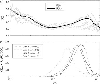
(figure 8
a).
 $\langle R_{f}^{\ast }\rangle _{c}$
reaches a local maximum between 0.2 and 0.45 for
 $0.5<Fr_{k}<0.9$
. We also define an overall mean irreversible flux Richardson number
 $\langle R_{f}^{\ast }\rangle _{all}$
as a function of
 $Fr_{k}$
by calculating the mean
 $R_{f}^{\ast }$
value among all cases in each
 $Fr_{k}$
bin. The
 $\langle R_{f}^{\ast }\rangle _{all}$
versus
 $Fr_{k}$
curve captures the general trends of the
 $\langle R_{f}^{\ast }\rangle _{c}$
versus
 $Fr_{k}$
results (figure 8
a). It reaches a local maximum of approximately 0.36 for
 $Fr_{k}\approx 0.7$
, where the balance of turbulence and stratification leads to the optimal mixing efficiency.
 $\langle R_{f}^{\ast }\rangle _{all}$
decreases as
 $Fr_{k}$
increases above 0.7 because there is less stratification to be mixed. As
 $Fr_{k}$
decreases below 0.7 until roughly 0.1,
 $\langle R_{f}^{\ast }\rangle _{all}$
decreases because the increased stratification suppresses turbulence. For
 $Fr_{k}<0.1$
,
 $\langle R_{f}^{\ast }\rangle _{all}$
increases as
 $Fr_{k}$
decreases because
 $\unicode[STIX]{x1D716}_{k}^{t}$
approaches zero. Despite the relatively large values of
 $\langle R_{f}^{\ast }\rangle _{c}$
for
 $Fr_{k}<0.1$
, only a small fraction of the total mixing occurs in these regions. This is evidenced by the result in figure 8(b), which shows the total irreversible mixing
 $\unicode[STIX]{x1D716}_{p}^{t}$
that occurs within each
 $Fr_{k}$
bin for cases 1, 3, 5 and 8.
We note that the data in this analysis are restricted to
 $4<ST_{L}<9$
and
 $100<Re_{L}<400$
, which is where the most total mixing occurs over the course of each breaking wave event. The
 $\langle R_{f}^{\ast }\rangle _{all}$
versus
 $Fr_{k}$
curve in figure 8(b) shows similarities to
 $R_{f}$
and
 $R_{f}^{\ast }$
versus
 $Fr_{k}$
relationships found in previous studies (Shih Reference Shih2003; Mater & Venayagamoorthy Reference Mater and Venayagamoorthy2014), particularly for
 $Fr_{k}>0.1$
. However, a complete analysis of
 $R_{f}^{\ast }$
in the (
 $ST_{L}$
,
 $Fr_{k}$
,
 $Re_{L}$
) parameter space, which would facilitate direct comparisons to these studies, is left to future work.
5 Volume-integrated energetics
5.1 Volume-integrated turbulent dissipation and mixing
By volume-integrating local dissipation and mixing quantities during wave breaking, we examine the changes in turbulent energetics as a function of the initial interface thickness
 $k\unicode[STIX]{x1D6FF}$
. We define the volume-integrated turbulent mixing as
 $$\begin{eqnarray}(\unicode[STIX]{x1D716}_{p}^{t})^{V}=\int _{V_{s}}\unicode[STIX]{x1D716}_{p}^{t}\,\text{d}V,\end{eqnarray}$$
where the volume of integration
 $V_{s}$
is defined as the sloping region of the domain (
 $L_{s}\leqslant x_{1}\leqslant L$
, see figure 1) in order to better isolate the effects of breaking (Arthur & Fringer Reference Arthur and Fringer2014). Maximum, cumulative and total volume-integrated turbulent mixing quantities are defined as
 $$\begin{eqnarray}\displaystyle (\unicode[STIX]{x1D716}_{p}^{t})_{max}^{V}=\max _{0\leqslant \unicode[STIX]{x1D70F}\leqslant \unicode[STIX]{x1D70F}_{f}}\left(\left(\unicode[STIX]{x1D716}_{p}^{t}\right)^{V}\right), & & \displaystyle\end{eqnarray}$$
 $$\begin{eqnarray}\displaystyle (\unicode[STIX]{x1D716}_{p}^{t})_{cum}^{V}=\int _{0}^{\unicode[STIX]{x1D70F}}\left(\unicode[STIX]{x1D716}_{p}^{t}\right)^{V}\text{d}\unicode[STIX]{x1D70F}, & & \displaystyle\end{eqnarray}$$
and
 $$\begin{eqnarray}(\unicode[STIX]{x1D716}_{p}^{t})_{tot}^{V}=\int _{0}^{\unicode[STIX]{x1D70F}_{f}}\left(\unicode[STIX]{x1D716}_{p}^{t}\right)^{V}\text{d}\unicode[STIX]{x1D70F},\end{eqnarray}$$
respectively. Similar quantities are defined for turbulent dissipation by replacing
 $\unicode[STIX]{x1D716}_{p}^{t}$
with
 $\unicode[STIX]{x1D716}_{k}^{t}$
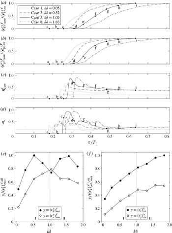
in (5.1)–(5.4). Turbulent dissipation and mixing both begin to rise after wave breaking occurs, and continue until the end of the breaking event
 $\unicode[STIX]{x1D70F}=\unicode[STIX]{x1D70F}_{f}$
(figure 9
a,b, points d–i for case 5). Note that the volume-integrated turbulent mixing efficiency measures in figure 9(c,d) are defined and discussed in § 5.3.
Volume-integrated turbulent energetics results for breaking wave cases 1–8. Shown are (a) cumulative dissipation
 $(\unicode[STIX]{x1D716}_{k}^{t})_{cum}^{V}$
, (b) cumulative mixing
 $(\unicode[STIX]{x1D716}_{p}^{t})_{cum}^{V}$
, (c) cumulative mixing efficiency
 $\unicode[STIX]{x1D702}_{cum}^{t}$
and (d) instantaneous mixing efficiency
 $\unicode[STIX]{x1D702}^{t}$
over time for cases 1, 3, 5 and 8. In (a) and (b),
 $(\unicode[STIX]{x1D716}_{k}^{t})_{cum}^{V}$
and
 $(\unicode[STIX]{x1D716}_{p}^{t})_{cum}^{V}$
are normalized by the total time-integrated values
 $(\unicode[STIX]{x1D716}_{k}^{t})_{tot}^{V}$
and
 $(\unicode[STIX]{x1D716}_{p}^{t})_{tot}^{V}$
, respectively. The critical
 $R_{f}$
value of 0.17 is shown by a horizontal dotted line in (c) and (d). Labels a–i in (a–d) correspond to the times shown in figure 2 for case 5. Also shown are (e) maximum and (f) total (time-integrated) values of dissipation and mixing as a function of
 $k\unicode[STIX]{x1D6FF}$
for all cases. Values in (e) are normalized by the maximum instantaneous turbulent dissipation for all cases
 $(\unicode[STIX]{x1D716}_{k}^{t})_{max}^{V,all}$
, while values in (f) are normalized by the maximum total turbulent dissipation for all cases
 $((\unicode[STIX]{x1D716}_{k}^{t})_{tot}^{V})_{max}^{all}$
. Vertical dotted lines in (e) and (f) represent
 $k\unicode[STIX]{x1D6FF}$
regimes I and II.

The variation in volume-integrated turbulent dissipation and mixing with
 $k\unicode[STIX]{x1D6FF}$
can be summarized by examining the maximum and total values of these quantities, as shown in figures 9(e) and 9(f), respectively. Here, we define two regimes of
 $k\unicode[STIX]{x1D6FF}$
based on the peaked shape of
 $(\unicode[STIX]{x1D716}_{p}^{t})_{max}^{V}$
(figure 9
e) and the asymptotic shape of
 $(\unicode[STIX]{x1D716}_{p}^{t})_{tot}^{V}$
(figure 9
f). Regime I is defined for
 $k\unicode[STIX]{x1D6FF}<1$
, where both
 $(\unicode[STIX]{x1D716}_{p}^{t})_{max}^{V}$
and
 $(\unicode[STIX]{x1D716}_{p}^{t})_{tot}^{V}$
increase monotonically. Regime II is defined for
 $k\unicode[STIX]{x1D6FF}\geqslant 1$
, where
 $(\unicode[STIX]{x1D716}_{p}^{t})_{max}^{V}$
decreases monotonically and
 $(\unicode[STIX]{x1D716}_{p}^{t})_{tot}^{V}$
asymptotes. The maximum volume-integrated turbulent dissipation
 $(\unicode[STIX]{x1D716}_{k}^{t})_{max}^{V}$
does not follow the peaked shape of
 $(\unicode[STIX]{x1D716}_{p}^{t})_{max}^{V}$
. Rather,
 $(\unicode[STIX]{x1D716}_{k}^{t})_{max}^{V}$
increases with
 $k\unicode[STIX]{x1D6FF}$
for low
 $k\unicode[STIX]{x1D6FF}$
values in regime I, and is relatively scattered as
 $k\unicode[STIX]{x1D6FF}$
increases into regime II. The total volume-integrated turbulent dissipation
 $(\unicode[STIX]{x1D716}_{k}^{t})_{tot}^{V}$
, however, increases monotonically with
 $k\unicode[STIX]{x1D6FF}$
through both regimes I and II.
5.2 Turbulent contribution to dissipation and mixing
Due to the computational restrictions associated with DNS, the Reynolds number
 $Re_{w}$
of our simulations is limited. In order to contextualize our results, it is therefore important to quantify the turbulent contribution to the full energy budget, which includes both laminar and turbulent effects. In this section, we use volume-integrated dissipation and mixing quantities to consider the turbulent contribution to the full dissipation and mixing that occurs during wave breaking. Scotti & White (Reference Scotti and White2014) define the local dissipation of the full kinetic energy as
 $$\begin{eqnarray}\unicode[STIX]{x1D716}_{k}=2\unicode[STIX]{x1D708}\unicode[STIX]{x1D61A}_{ij}\unicode[STIX]{x1D61A}_{ji},\end{eqnarray}$$
where
 $\unicode[STIX]{x1D61A}_{ij}=((\unicode[STIX]{x2202}u_{i}/\unicode[STIX]{x2202}x_{j})+(\unicode[STIX]{x2202}u_{j}/\unicode[STIX]{x2202}x_{i}))/2$
is the rate of strain tensor, see (1.1) therein. Thus, we define the full volume-integrated dissipation as
 $$\begin{eqnarray}{\mathcal{D}}=\int _{V_{s}}\unicode[STIX]{x1D716}_{k}\,\text{d}V,\end{eqnarray}$$
where the volume of integration
 $V_{s}$
is defined as in § 5.1. We define the full volume-integrated mixing as in Winters et al. (Reference Winters, Lombard, Riley and D’Asaro1995),
 $$\begin{eqnarray}{\mathcal{M}}=\frac{\unicode[STIX]{x1D705}g}{\unicode[STIX]{x1D70C}_{0}}\left(\int _{V_{s}}x_{3}^{\ast }\frac{\unicode[STIX]{x2202}^{2}}{\unicode[STIX]{x2202}x_{j}\unicode[STIX]{x2202}x_{j}}\unicode[STIX]{x1D70C}(x_{3}^{\ast })\,\text{d}V-\int _{A}(\unicode[STIX]{x1D70C}_{top}-\unicode[STIX]{x1D70C}_{bottom})\,\text{d}A\right)=\unicode[STIX]{x1D719}_{d}-\unicode[STIX]{x1D719}_{i},\end{eqnarray}$$
where
 $\unicode[STIX]{x1D719}_{d}$
is the volume-integrated rate of change in the background potential energy and
 $\unicode[STIX]{x1D719}_{i}$
is the irreversible rate of change from internal to potential energy. Here,
 $\unicode[STIX]{x1D70C}_{top}$
and
 $\unicode[STIX]{x1D70C}_{bottom}$
are the densities on the top and bottom boundaries of the domain, respectively, and
 $A$
is the corresponding surface area of the boundary. We note that the full volume-integrated dissipation
 ${\mathcal{D}}$
and mixing
 ${\mathcal{M}}$
measures defined here are equal to those used previously by Arthur & Fringer (Reference Arthur and Fringer2014). The dissipation
 $\unicode[STIX]{x1D716}$
in Arthur & Fringer (Reference Arthur and Fringer2014) is equal to
 ${\mathcal{D}}$
and the effective irreversible mixing
 $\unicode[STIX]{x1D719}_{e}$
in Arthur & Fringer (Reference Arthur and Fringer2014) is equal to
 ${\mathcal{M}}$
. The values
 ${\mathcal{D}}$
and
 ${\mathcal{M}}$
include both laminar and turbulent effects, while
 $(\unicode[STIX]{x1D716}_{k}^{t})^{V}$
and
 $(\unicode[STIX]{x1D716}_{p}^{t})^{V}$
(5.1) include only turbulent effects.
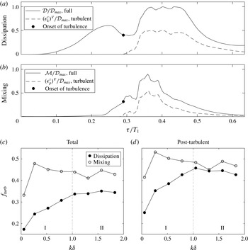
The turbulent contribution to dissipation and mixing. Volume-integrated (a) dissipation (
 $(\unicode[STIX]{x1D716}_{k}^{t})^{V}$
, turbulent and
 ${\mathcal{D}}$
, full) and (b) mixing (
 $(\unicode[STIX]{x1D716}_{p}^{t})^{V}$
, turbulent and
 ${\mathcal{M}}$
, full) over time for breaking wave case 5 (
 $k\unicode[STIX]{x1D6FF}\approx 1$
). Values in (a) and (b) are normalized by
 ${\mathcal{D}}_{max}$
, the maximum full dissipation for case 5. The fraction
 $f_{turb}$
of both dissipation and mixing (c) over the entire breaking wave event (‘Total’) and (d) during the turbulent portion of the event (‘Post-turbulent’), as a function of
 $k\unicode[STIX]{x1D6FF}$
for all cases. The vertical dotted lines in (c) and (d) represent
 $k\unicode[STIX]{x1D6FF}$
regimes I and II defined in § 5.1.

The initial peak in the full dissipation
 ${\mathcal{D}}$
(shown for case 5 in figure 10
a) is associated with near-bottom downslope flow in the lower layer prior to breaking (figure 2
a). As noted in Arthur & Fringer (Reference Arthur and Fringer2014), this dissipation is laminar because turbulence does not develop in the domain until wave breaking occurs. The turbulent dissipation
 $(\unicode[STIX]{x1D716}_{k}^{t})^{V}$
, therefore, does not begin to rise until breaking and does not include this pre-breaking laminar dissipation. The shapes of the turbulent mixing
 $(\unicode[STIX]{x1D716}_{p}^{t})^{V}$
and full mixing
 ${\mathcal{M}}$
curves (shown for case 5 in figure 10
b) are similar. This is expected because the turbulence generated by overturning during the breaking event is the primary driver of mixing in the domain. Overall, however,
 $(\unicode[STIX]{x1D716}_{k}^{t})^{V}$
and
 $(\unicode[STIX]{x1D716}_{p}^{t})^{V}$
are generally lower than
 ${\mathcal{D}}$
and
 ${\mathcal{M}}$
, respectively, throughout the breaking event.
In order to quantify the difference between the turbulent and full measures of dissipation and mixing, we define
 $f_{turb}$
as the fraction of either dissipation or mixing due to turbulence over the course of the breaking event. Thus
 $f_{turb}=(\unicode[STIX]{x1D716}_{k}^{t})_{tot}^{V}/{\mathcal{D}}_{tot}$
for dissipation and
 $f_{turb}=(\unicode[STIX]{x1D716}_{p}^{t})_{tot}^{V}/{\mathcal{M}}_{tot}$
for mixing, where
 ${\mathcal{D}}_{tot}$
and
 ${\mathcal{M}}_{tot}$
are the time-integrated values of
 ${\mathcal{D}}$
and
 ${\mathcal{M}}$
, respectively, defined as in (5.4) for
 $(\unicode[STIX]{x1D716}_{p}^{t})_{tot}^{V}$
. The turbulent contribution to dissipation (figure 10
c) increases within regime I from approximately 17 % for case 1 to approximately 35 % for case 5 (
 $k\unicode[STIX]{x1D6FF}\approx 1$
). Within regime II,
 $f_{turb}$
remains relatively constant. The turbulent contribution to mixing (figure 10
c) is approximately 34 % for case 1, but is then roughly constant between 40 %–50 % for larger
 $k\unicode[STIX]{x1D6FF}$
. The onset of turbulence in the domain (when
 $(\unicode[STIX]{x1D716}_{k}^{t})^{V}$
and
 $(\unicode[STIX]{x1D716}_{p}^{t})^{V}$
begin to rise) is indicated by a dot in figure 10(a,b). Another calculation of
 $f_{turb}$
, this time over only the post-turbulent portion of the event (as opposed to the entire event) is shown in figure 10(d). The turbulent contributions to dissipation and mixing are higher in the post-turbulent stage because the laminar pre-breaking stage is not included, reaching approximately 45 % for dissipation and 45 %–55 % for mixing. However, similar trends are seen with
 $k\unicode[STIX]{x1D6FF}$
.
Overall, the turbulent contribution to dissipation and mixing is relatively low (
 ${<}60$
%). This is a consequence of the low Reynolds number
 $Re_{w}$
used in our simulations, which is necessitated by the computational restrictions associated with DNS. Although we reach local
 $Re_{b}$
values of the order of
 $10^{2}{-}10^{3}$
(in the energetic regime of Shih et al.
Reference Shih, Koseff, Ivey and Ferziger2005), these regions make up only a small fraction of the domain. Arthur & Fringer (Reference Arthur and Fringer2014) found that as
 $Re_{w}$
increases, the turbulent contribution to dissipation and mixing during breaking internal wave events increases because turbulence develops earlier in the event. Thus, we expect that as the Reynolds number of the cases considered in this study increases, the turbulent contribution to dissipation and mixing will also increase. The potential effect of increasing the Reynolds number on the mixing efficiency is discussed in the next section. However, further analysis at larger Reynolds number is left to future work.
5.3 Volume-integrated mixing efficiency
Using the volume-integrated calculations of turbulent dissipation and mixing above, volume-integrated measures of the turbulent mixing efficiency are made. We define a cumulative volume-integrated turbulent mixing efficiency
 $$\begin{eqnarray}\unicode[STIX]{x1D702}_{cum}^{t}(\unicode[STIX]{x1D70F})=\frac{\displaystyle \int _{0}^{\unicode[STIX]{x1D70F}}(\unicode[STIX]{x1D716}_{p}^{t})^{V}\,\text{d}\unicode[STIX]{x1D70F}}{\displaystyle \int _{0}^{\unicode[STIX]{x1D70F}}\left((\unicode[STIX]{x1D716}_{p}^{t})^{V}+(\unicode[STIX]{x1D716}_{k}^{t})^{V}\right)\text{d}\unicode[STIX]{x1D70F}},\end{eqnarray}$$
as well as a bulk volume-integrated turbulent mixing efficiency
 $$\begin{eqnarray}\unicode[STIX]{x1D702}_{B}^{t}=\frac{(\unicode[STIX]{x1D716}_{p}^{t})_{tot}^{V}}{(\unicode[STIX]{x1D716}_{p}^{t})_{tot}^{V}+(\unicode[STIX]{x1D716}_{k}^{t})_{tot}^{V}}.\end{eqnarray}$$
Thus,
 $\unicode[STIX]{x1D702}_{cum}^{t}(\unicode[STIX]{x1D70F}_{f})=\unicode[STIX]{x1D702}_{B}^{t}$
. As in Arthur & Fringer (Reference Arthur and Fringer2014), we also define a full bulk mixing efficiency, which includes both laminar and turbulent effects, as
 $$\begin{eqnarray}\unicode[STIX]{x1D702}_{B}=\frac{{\mathcal{M}}_{tot}}{{\mathcal{M}}_{tot}+{\mathcal{D}}_{tot}}.\end{eqnarray}$$
The cumulative mixing efficiency
 $\unicode[STIX]{x1D702}_{cum}^{t}$
(figure 9
c) is initially large due to the offset between the growth of mixing and dissipation in the early stages of turbulence. That is, as sharp density surfaces are created by turbulent strain, mixing begins to increase before turbulent dissipation occurs. This effect is discussed in Smyth et al. (Reference Smyth, Moum and Caldwell2001), who observed a similar phenomenon in stratified shear flow turbulence. After turbulence has developed,
 $\unicode[STIX]{x1D702}_{cum}^{t}$
decreases, approaching
 $\unicode[STIX]{x1D702}_{B}^{t}$
. The bulk volume-integrated turbulent mixing efficiency
 $\unicode[STIX]{x1D702}_{B}^{t}$
varies in the
 $k\unicode[STIX]{x1D6FF}$
regimes defined in § 5.1 (figure 11).
 $\unicode[STIX]{x1D702}_{B}^{t}$
is low (roughly 0.25) for small
 $k\unicode[STIX]{x1D6FF}$
(case 1). As
 $k\unicode[STIX]{x1D6FF}$
increases within regime I, the mixing efficiency increases, reaching a peak of 0.37 when
 $k\unicode[STIX]{x1D6FF}\approx 1$
(case 5). Within regime II,
 $\unicode[STIX]{x1D702}_{B}^{t}$
levels out around 0.35.
Bulk mixing efficiency measures
 $\unicode[STIX]{x1D702}_{B}^{t}$
and
 $\unicode[STIX]{x1D702}_{B}$
as functions of
 $k\unicode[STIX]{x1D6FF}$
. The vertical dotted line represents
 $k\unicode[STIX]{x1D6FF}$
regimes I and II defined in § 5.1. Also shown are the bulk mixing efficiency results of Fringer & Street (Reference Fringer and Street2003).

The volume-integrated bulk mixing efficiency values calculated for breaking wave cases 1–8 are consistently higher than the critical value of the flux Richardson number,
 $R_{f}^{crit}\approx 0.17$
. However, we note that the instantaneous volume-integrated turbulent mixing efficiency, defined as
 $$\begin{eqnarray}\unicode[STIX]{x1D702}^{t}(\unicode[STIX]{x1D70F})=\frac{(\unicode[STIX]{x1D716}_{p}^{t})^{V}}{(\unicode[STIX]{x1D716}_{p}^{t})^{V}+(\unicode[STIX]{x1D716}_{k}^{t})^{V}},\end{eqnarray}$$
and shown in figure 9(d), does approach
 $R_{f}^{crit}\approx 0.17$
towards the end of the breaking event, especially for low values of
 $k\unicode[STIX]{x1D6FF}$
. This asymptotic behaviour occurs for each case, indicating that the turbulence after breaking reaches an equilibrium state representative of what one might expect in turbulence that is predominantly shear driven. A similar trend was observed by Smyth et al. (Reference Smyth, Moum and Caldwell2001) for the flux coefficient, which is analogous to the mixing efficiency.
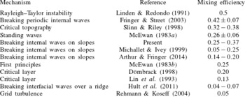
Mixing efficiency values from previous studies.

For further comparison to the present results, table 2 shows mixing efficiency values that have been calculated for various flows in previous studies. It is similar to table 1 in Fringer & Street (Reference Fringer and Street2003), but with the addition of several more recent studies. The range of bulk turbulent mixing efficiency values calculated here (
 $\unicode[STIX]{x1D702}_{B}^{t}=0.25-0.37$
) is on the upper end of the values reported in other studies of breaking internal waves on slopes (Michallet & Ivey Reference Michallet and Ivey1999; Arthur & Fringer Reference Arthur and Fringer2014). This may be because we consider only the turbulent contribution to the bulk mixing efficiency, as discussed in § 5.2. For the relatively low Reynolds number in our simulations, laminar dissipation occurs due to strong downslope flow near the bottom boundary prior to wave breaking. This laminar dissipation reduces the overall mixing efficiency of the breaking event
 $\unicode[STIX]{x1D702}_{B}$
(see figure 11), but is not captured in
 $\unicode[STIX]{x1D702}_{B}^{t}$
, which includes only turbulent effects. At higher Reynolds number, we would expect turbulence to develop earlier in the simulation (i.e. during the downslope flow of lower-layer fluid before breaking), increasing turbulent dissipation and thus lowering the turbulent mixing efficiency. Therefore, at increased Reynolds number, we would expect
 $\unicode[STIX]{x1D702}_{B}^{t}$
and
 $\unicode[STIX]{x1D702}_{B}$
to approach one another because the turbulent contribution to dissipation and mixing would overwhelm the laminar contribution.
The bulk mixing efficiency values calculated here are also larger than those presented by Hult et al. (Reference Hult, Troy and Koseff2011) for breaking internal waves over a ridge. This is due, in part, to the presence of turbulence in the unstratified bottom boundary layer of their domain. Conversely, in the present breaking wave cases, the stratified region intersects the bottom boundary layer on the slope, allowing for near-bottom mixing. Because the method of Scotti & White (Reference Scotti and White2014) defines turbulent dissipation and mixing locally,
 $\unicode[STIX]{x1D716}_{k}^{t}$
and
 $\unicode[STIX]{x1D716}_{p}^{t}$
can be integrated over the bottom boundary and interior regions separately. We define the bottom boundary layer as in § 2.1 as
 $x_{3}<-d+\unicode[STIX]{x1D6FF}_{S}$
, where
 $d$
is the local depth, and the interior as the remainder of the domain. Although we find that 80 %–90 % of the total dissipation and mixing occur in the interior region, the bulk turbulent mixing efficiencies in both layers are similar to the overall value
 $\unicode[STIX]{x1D702}_{B}^{t}$
(see Arthur Reference Arthur2015).
The present bulk mixing efficiency values are lower than those calculated by Fringer & Street (Reference Fringer and Street2003) for breaking progressive internal waves in deep water because of the absence of bottom boundary-layer dissipation in their domain. Fringer & Street (Reference Fringer and Street2003) also found a different shape of the bulk mixing efficiency as a function of
 $k\unicode[STIX]{x1D6FF}$
(see figure 11). In their study,
 $ka$
is relatively large; this allows
 $k\unicode[STIX]{x1D6FF}$
to control the mixing efficiency because billows are not restricted in size by
 $ka$
. Thus, weak convective breaking occurs for large
 $k\unicode[STIX]{x1D6FF}$
, causing the mixing efficiency to decrease. In our simulations,
 $ka$
is relatively small. Thus, the mixing efficiency is controlled by
 $ka$
for large
 $k\unicode[STIX]{x1D6FF}$
(regime II), and is relatively constant. For further discussion of the billow scale in our breaking wave cases, see § 6 below.
An important consideration when comparing the present mixing efficiency calculations to those of other flows, especially in the laboratory or the field, is the Prandtl number
 $Pr=\unicode[STIX]{x1D708}/\unicode[STIX]{x1D705}$
. In water,
 $Pr=7$
for temperature and
 $Pr=700$
for salt. As
 $Pr$
increases (
 $\unicode[STIX]{x1D705}$
decreases), one would expect the mixing efficiency to decrease because the time scale necessary for mixing to occur increases. However,
 $Pr=1$
in the current simulations due to the computational restrictions associated with resolving mixing for smaller values of
 $\unicode[STIX]{x1D705}$
. This provides another potential explanation for the relatively high mixing efficiencies in the present study.
5.4 Numerical effects
Numerical effects also play a role in the energetics, and are a function of the chosen numerical methods and discretization. There are, in fact, three sources of dissipation in our simulations: that due to mean (or laminar) strains, that due to turbulent strains and that due to numerical effects. We estimate the relative magnitude of the numerical dissipation, in a domain- and time-integrated sense, by comparing the change in total energy over the course of each simulation to that captured by resolved quantities. Following Winters et al. (Reference Winters, Lombard, Riley and D’Asaro1995) and Arthur & Fringer (Reference Arthur and Fringer2014), the total energy is defined as
 $$\begin{eqnarray}E_{T}=\frac{1}{2}\int _{V_{d}}u_{i}u_{i}\,\text{d}V+\frac{g}{\unicode[STIX]{x1D70C}_{0}}\int _{V_{d}}\unicode[STIX]{x1D70C}x_{3}\,\text{d}V=E_{K}+E_{P},\end{eqnarray}$$
where
 $V_{d}$
is the full volume of the domain,
 $E_{K}$
is the kinetic energy and
 $E_{P}$
is the potential energy. The evolution of
 $E_{T}$
should satisfy
 $$\begin{eqnarray}\frac{\text{d}E_{T}}{\text{d}\unicode[STIX]{x1D70F}}=\unicode[STIX]{x1D719}_{i}-{\mathcal{D}}\end{eqnarray}$$
because there are no boundary fluxes (Winters et al. Reference Winters, Lombard, Riley and D’Asaro1995). Numerical dissipation can therefore be estimated as the difference between the total energy change and the resolved energy change,
 $$\begin{eqnarray}{\mathcal{N}}_{cum}=\int _{0}^{\unicode[STIX]{x1D70F}}\left(\frac{\text{d}E_{T}}{\text{d}\unicode[STIX]{x1D70F}}-\unicode[STIX]{x1D719}_{i}+{\mathcal{D}}\right)\text{d}\unicode[STIX]{x1D70F}=\unicode[STIX]{x0394}E_{T}-\unicode[STIX]{x1D719}_{i,cum}+{\mathcal{D}}_{cum}.\end{eqnarray}$$
As shown in figure 12(a) for case 1, the majority of the numerical dissipation occurs prior to wave breaking (
 $\unicode[STIX]{x1D70F}/T_{1}<0.2$
), as the initial wave evolves on the coarse, offshore portion of the grid.
(a) Cumulatively integrated
 $E_{T}$
evolution terms from (5.14) over time for case 1, normalized by
 $({\mathcal{M}}_{tot}+{\mathcal{D}}_{tot})$
. (b) Domain- and time-integrated estimate of numerical dissipation
 ${\mathcal{N}}_{tot}$
relative to the resolved full dissipation and mixing
 $({\mathcal{M}}_{tot}+{\mathcal{D}}_{tot})$
, as a function of
 $k\unicode[STIX]{x1D6FF}$
.

The total domain- and time-integrated numerical dissipation can be estimated as
 ${\mathcal{N}}_{tot}={\mathcal{N}}_{cum}(\unicode[STIX]{x1D70F}_{f})$
, allowing us to estimate the effect of numerical dissipation on the full bulk mixing efficiency
 $\unicode[STIX]{x1D702}_{B}$
(5.10). We define an effective full bulk mixing efficiency as
 $$\begin{eqnarray}\displaystyle \unicode[STIX]{x1D702}_{B,eff} & & \displaystyle =\frac{{\mathcal{M}}_{tot}}{{\mathcal{M}}_{tot}+{\mathcal{D}}_{tot}+{\mathcal{N}}_{tot}},\end{eqnarray}$$
 $$\begin{eqnarray}\displaystyle & & \displaystyle =\frac{{\mathcal{M}}_{tot}}{{\mathcal{M}}_{tot}+{\mathcal{D}}_{tot}\left(1+\displaystyle \frac{{\mathcal{N}}_{tot}}{{\mathcal{M}}_{tot}+{\mathcal{D}}_{tot}}\right)},\end{eqnarray}$$
 $$\begin{eqnarray}\displaystyle & & \displaystyle =\frac{\unicode[STIX]{x1D702}_{B}}{1+\displaystyle \frac{{\mathcal{N}}_{tot}}{{\mathcal{M}}_{tot}+{\mathcal{D}}_{tot}}}.\end{eqnarray}$$
Because
 $1/(1-r)=1+r+r^{2}/2+\cdots \,$
, equation (5.17) can be simplified to
 $$\begin{eqnarray}\unicode[STIX]{x1D702}_{B,eff}\approx \unicode[STIX]{x1D702}_{B}\left(1-\frac{{\mathcal{N}}_{tot}}{{\mathcal{M}}_{tot}+{\mathcal{D}}_{tot}}\right).\end{eqnarray}$$
For cases 2–8, the quantity
 $|{\mathcal{N}}_{tot}/({\mathcal{M}}_{tot}+{\mathcal{D}}_{tot})|$
varies between 0.06–0.11 (figure 12
b), indicating that
 $\unicode[STIX]{x1D702}_{B,eff}$
is within approximately 6 %–11 % of
 $\unicode[STIX]{x1D702}_{B}$
. For case 1, which has the smallest value of
 $k\unicode[STIX]{x1D6FF}$
, the value of
 ${\mathcal{N}}_{tot}/({\mathcal{M}}_{tot}+{\mathcal{D}}_{tot})$
is slightly larger in magnitude (approximately 0.2). However, as noted above in reference to figure 12(a), the majority of the numerical dissipation occurs prior to wave breaking. Although case 1 is shown in figure 12(a) because it has the largest amount of numerical dissipation, cases 2–8 show qualitatively similar results as a function of time. The overall findings of this paper related to the bulk mixing efficiency would not change despite the relatively large effect of numerical dissipation in case 1. In particular, the numerical dissipation would act to further decrease the bulk mixing efficiency for case 1, which already possesses the smallest bulk mixing efficiency among all cases.
The numerical dissipation in our simulations is due to the non-conservative energy behaviour of non-staggered grid methods, which do not allow the discrete form of the energy flux related to
 $pu_{i}$
(where
 $p$
is the pressure) to be written in conservative form (Ferziger & Perić Reference Ferziger and Perić2002). It is therefore related to the projection scheme used by Zang et al. (Reference Zang, Street and Koseff1994) and not to numerical diffusion of momentum, which is expected because momentum advection is computed with the dispersive QUICK scheme (Leonard Reference Leonard1979). Based on numerical tests (not shown),
 $\unicode[STIX]{x1D719}_{i}$
and
 ${\mathcal{D}}$
are relatively weak functions of the grid spacing and time step size, while
 ${\mathcal{N}}$
is a relatively strong function of these parameters. This suggests that if we had the computational resources to perform the simulations with higher resolution and a smaller time step size, the effective bulk mixing efficiency
 $\unicode[STIX]{x1D702}_{B,eff}$
would converge to the reported bulk mixing efficiency
 $\unicode[STIX]{x1D702}_{B}$
. Such higher-resolution simulations would also allow for a grid-resolution study of the dissipation spectra, a more rigorous method for assessing numerical dissipation.
6 Connecting local and volume-integrated energetics
Thus far, we have calculated both local and volume-integrated measures of turbulent energetics and mixing efficiency during breaking internal wave events on slopes. The local turbulent mixing efficiency (in terms of
 $\langle R_{f}^{\ast }\rangle _{c}$
) varies with the local turbulent Froude number
 $Fr_{k}$
. However, there is no clear dependence of the
 $\langle R_{f}^{\ast }\rangle _{c}$
versus
 $Fr_{k}$
curves on the initial interface thickness
 $k\unicode[STIX]{x1D6FF}$
, as they all generally follow
 $\langle R_{f}^{\ast }\rangle _{all}$
(figure 8
a). Alternatively, the bulk turbulent mixing efficiency
 $\unicode[STIX]{x1D702}_{B}^{t}$
does depend on
 $k\unicode[STIX]{x1D6FF}$
(figure 11).
Ultimately, we seek to explain the dependence of
 $\unicode[STIX]{x1D702}_{B}^{t}$
on
 $k\unicode[STIX]{x1D6FF}$
by understanding how
 $k\unicode[STIX]{x1D6FF}$
affects the local turbulence that drives mixing. We hypothesize that because
 $\unicode[STIX]{x1D702}_{B}^{t}$
depends on the total mixing that occurs over the course of a breaking event, it should be related to the turbulent Froude number
 $Fr_{k}$
at which the maximum fraction of the total mixing occurs. We therefore define
 $Fr_{k}^{max}$
as the value of
 $Fr_{k}$
corresponding to the peak of the
 $(\sum _{Fr_{k}}\unicode[STIX]{x1D716}_{p}^{t}A_{cell}W)/(\unicode[STIX]{x1D716}_{p}^{t})_{tot}^{V}$
versus
 $Fr_{k}$
curves shown in figure 8(b). As presented in figure 13(a),
 $Fr_{k}^{max}$
is indeed related to
 $k\unicode[STIX]{x1D6FF}$
;
 $Fr_{k}^{max}$
generally increases with
 $k\unicode[STIX]{x1D6FF}$
as the background stratification decreases. Furthermore,
 $Fr_{k}^{max}$
can be used to predict the bulk turbulent mixing efficiency
 $\unicode[STIX]{x1D702}_{B}^{t}$
for cases 1–8 (figure 13
b).
 $\unicode[STIX]{x1D702}_{B}^{t}$
is maximized when
 $Fr_{k}^{max}\approx 0.4$
.
(a) The
 $Fr_{k}$
of maximum mixing
 $Fr_{k}^{max}$
as a function of
 $k\unicode[STIX]{x1D6FF}$
and (b) the bulk turbulent mixing efficiency
 $\unicode[STIX]{x1D702}_{B}^{t}$
as a function of
 $Fr_{k}^{max}$
. The vertical dotted line in (a) represents
 $k\unicode[STIX]{x1D6FF}$
regimes I and II defined in § 5.1.

Physically, the control that
 $k\unicode[STIX]{x1D6FF}$
places on
 $Fr_{k}^{max}$
can be described in terms of the vertical length scale of the billows that form at the density interface during wave breaking. We define
 $L_{b}(x_{1})$
as the vertical length scale of the region defined by
 $Re_{L}>100$
at the time of maximum volume-integrated turbulent mixing
 $(\unicode[STIX]{x1D716}_{p}^{t})_{max}^{V}$
. This region is shown in figure 14(a–c) for cases 1, 5 and 8, respectively. For each case, the height of the upslope surge above the bottom boundary at this time is approximately equal to
 $a$
, the incoming wave amplitude (indicated by the dashed line in figure 14
a–c). We therefore normalize
 $L_{b}^{max}$
by
 $2a$
in figure 14(d,e) in order to determine when the billow scale is affected by the bottom.
The vertical length scale
 $L_{b}$
of the billows at the interface at the time of maximum volume-integrated turbulent mixing
 $(\unicode[STIX]{x1D716}_{p}^{t})_{max}^{V}$
. (a–c) The region defined by
 $Re_{L}>100$
that encompasses the billows for cases 1, 5 and 8, respectively. The dashed line shows the approximate height of the upslope surge above the bottom, which is approximately equal to the incoming wave amplitude
 $a$
. (d)
 $L_{b}^{max}/2a$
as a function of
 $k\unicode[STIX]{x1D6FF}$
for all cases. The vertical dotted line represents
 $k\unicode[STIX]{x1D6FF}$
regimes I and II defined in § 5.1. (e)
 $L_{b}^{max}/2a$
as a function of
 $Fr_{k}^{max}$
for all cases.

For small
 $k\unicode[STIX]{x1D6FF}$
,
 $L_{b}$
is controlled by the thickness of the interface because billows are confined to the thin stratified region (figure 14
a). Thus,
 $L_{b}^{max}/2a<1$
(figure 14
d, regime I), and
 $Fr_{k}^{max}$
is relatively small (figure 14
e). As
 $k\unicode[STIX]{x1D6FF}$
increases and the interface thickens,
 $L_{b}^{max}/2a$
and thus
 $Fr_{k}^{max}$
increase as well. For case 5 (
 $k\unicode[STIX]{x1D6FF}\approx 1$
),
 $L_{b}^{max}/2a\approx 1$
and
 $Fr_{k}^{max}\approx 0.4$
, indicating the optimal transfer of energy from the large-scale wave into the billows that generate turbulence (figure 14
b), and thus the maximum bulk mixing efficiency. As
 $k\unicode[STIX]{x1D6FF}$
increases above 1, the billows continue to grow in scale (figure 14
c). The vertical scale
 $L_{b}^{max}/2a$
increases above 1 (figure 14
d, regime II) and
 $Fr_{k}^{max}$
increases above the optimal value of approximately 0.4. In regime II, The billows are clearly affected by the bottom, as
 $L_{b}^{max}/2a>1$
. This restriction on the billow scale likely leads to the asymptotic trend in the bulk mixing efficiency measures
 $\unicode[STIX]{x1D702}_{B}^{t}$
and
 $\unicode[STIX]{x1D702}_{B}$
seen in figure 11. As
 $k\unicode[STIX]{x1D6FF}$
increases above the values considered in this study, we would expect
 $L_{b}^{max}/2a$
to asymptote and
 $Fr_{k}^{max}$
to increase, leading to a decrease in the bulk mixing efficiency. However, we note that the increase in
 $k\unicode[STIX]{x1D6FF}$
was limited in order to keep the other relevant non-dimensional parameters (
 $ka$
and
 $Re_{w}$
) relatively fixed (see § 2.2).
7 Conclusions
Using DNS, we have explored local and volume-integrated measures of turbulence and mixing in breaking internal waves on slopes. We considered eight breaking wave cases with a range of normalized pycnocline thicknesses
 $k\unicode[STIX]{x1D6FF}$
, but with similar incoming wave properties (
 $ka$
,
 $Re_{w}$
). Thus, for a similar incoming wave and constant bathymetric slope, we examined the effect of stratification on energetics and mixing efficiency. This effect is relevant in lakes and the coastal ocean, where the stratification supporting internal wave motion may change on daily or seasonal time scales. We began with a physical description of wave breaking as a function of
 $k\unicode[STIX]{x1D6FF}$
. The breaking process is similar for all cases, and agrees with the description in Arthur & Fringer (Reference Arthur and Fringer2014). A collapsing breaker leads to an upslope surge of dense fluid, during which turbulence is generated in regions of unstable stratification within billows at the interface and underneath the nose of the upslope surge.
The local irreversible mixing efficiency
 $R_{f}^{\ast }$
was found to vary between 0 and 1 throughout the turbulent region of the flow. It was relatively large in the billow roll-up regions and at the nose of the upslope surge, where
 $\unicode[STIX]{x1D716}_{p}^{t}$
was elevated, and smaller within the billow cores and throughout the rest of the turbulent region. The bulk (spatially and time-averaged)
 $R_{f}^{\ast }$
was found to be approximately 0.3 for each case, indicating little variation with the initial interface thickness
 $k\unicode[STIX]{x1D6FF}$
. Using the parameter space of Mater & Venayagamoorthy (Reference Mater and Venayagamoorthy2014) and restricting the data to the
 $Re_{L}$
and
 $ST_{L}$
of maximum turbulent mixing, the mean irreversible flux Richardson number
 $\langle R_{f}^{\ast }\rangle _{c}$
was found to vary with the turbulent Froude number
 $Fr_{k}$
for each case. However, the
 $\langle R_{f}^{\ast }\rangle _{c}$
versus
 $Fr_{k}$
curves showed no clear dependence on
 $k\unicode[STIX]{x1D6FF}$
. Their trends were captured by an overall mean irreversible flux Richardson number
 $\langle R_{f}^{\ast }\rangle _{all}$
that reached a local maximum of approximately 0.36 for
 $Fr_{k}\approx 0.7$
, where the balance of turbulence and stratification leads to the optimal mixing efficiency.
Unlike the local turbulent mixing efficiency measures based on
 $R_{f}^{\ast }$
, the volume-integrated turbulent mixing efficiency
 $\unicode[STIX]{x1D702}_{B}^{t}$
was found to vary with
 $k\unicode[STIX]{x1D6FF}$
, ranging from 0.25 for low
 $k\unicode[STIX]{x1D6FF}$
to a maximum of 0.37 for
 $k\unicode[STIX]{x1D6FF}\approx 1$
. For
 $k\unicode[STIX]{x1D6FF}>1$
,
 $\unicode[STIX]{x1D702}_{B}^{t}\approx 0.35$
. In order to explain the variation in
 $\unicode[STIX]{x1D702}_{B}^{t}$
with
 $k\unicode[STIX]{x1D6FF}$
based on the state of turbulence during wave breaking, we showed that
 $Fr_{k}^{max}$
, the Froude number at which the maximum turbulent mixing occurs over the course of a breaking event, can be used to predict
 $\unicode[STIX]{x1D702}_{B}^{t}$
, which is maximized for
 $Fr_{k}^{max}\approx 0.4$
. Physically, we found that
 $Fr_{k}^{max}$
is controlled by the vertical length scale of billows at the interface during wave breaking.
We note that our findings are limited by the chosen parameter space, wherein the interface thickness
 $k\unicode[STIX]{x1D6FF}$
was varied, but the wave steepness
 $ka$
and the bathymetric slope
 $s$
remained constant. Previous studies (Boegman et al.
Reference Boegman, Ivey and Imberger2005; Venayagamoorthy & Fringer Reference Venayagamoorthy and Fringer2007; Aghsaee et al.
Reference Aghsaee, Boegman and Lamb2010; Arthur & Fringer Reference Arthur and Fringer2014) have shown that wave breaking dynamics and energetics change with wave amplitude and bathymetric slope. Additionally, due to computational restrictions, we have limited our results to
 $Pr=1$
and a relatively low wave Reynolds number
 $Re_{w}\approx 150$
, which are not realistic in a geophysical sense. Future work on turbulence and mixing in breaking internal waves on slopes should address these limitations by exploring a wider parameter space.
Acknowledgements
R.S.A. gratefully acknowledges the support of the Stanford Graduate Fellowship (SGF). R.S.A. and O.B.F. gratefully acknowledge the support of ONR grant N00014-08-1-0904 (scientific officers Dr C. L. Vincent, Dr T. Paluszkiewicz and Dr S. Harper). We gratefully acknowledge the US Army Research Laboratory DoD Supercomputing Resource Center for computer time on Pershing and Excalibur and especially thank the diligent staff at the HPC Help Desk for their support. We also thank O. Murray of ONR for ensuring our access to these resources. Finally, we thank K. S. Nelson for helpful discussions, and three anonymous referees for their thoughtful reviews of the manuscript.