1 Introduction
Kohn–Sham density functional theory (Hohenberg and Kohn Reference Hohenberg and Kohn1964, Kohn and Sham Reference Kohn and Sham1965) (DFT) is today the most widely used electronic structure theory in chemistry, materials science and other related fields, and was recognized by the Nobel Prize in Chemistry awarded to Walter Kohn in 1998. Despite being developed in the mid-1960s, Kohn–Sham DFT was not a popular approach until the beginning of the 1980s, when practical exchange-correlation functionals obtained from quantum Monte Carlo calculations (Ceperley and Alder Reference Ceperley and Alder1980, Perdew and Zunger Reference Perdew and Zunger1981) became available. Together with the development of more advanced exchange-correlation functionals (e.g. Lee, Yang and Parr Reference Lee, Yang and Parr1988, Becke Reference Becke1993, Perdew, Burke and Ernzerhof Reference Perdew, Burke and Ernzerhof1996a , Heyd, Scuseria and Ernzerhof Reference Heyd, Scuseria and Ernzerhof2003), Kohn–Sham DFT has been demonstrated to be capable of predicting chemical and material properties for a wide range of systems from first principles. More specifically, under the Born–Oppenheimer approximation that the nuclei are treated as classical particles, in principle the only input needed for Kohn–Sham DFT calculations is the most basic information concerning the system: atomic species and atomic positions.
The success of Kohn–Sham DFT cannot be separated from the vast improvement in numerical algorithms and computer architecture, particularly during the 1980s and 1990s. Some relatively basic ideas, such as using the conjugate gradient method for solving eigenvalue problems (Payne et al. Reference Payne, Teter, Allen, Arias and Joannopoulos1992), efficient use of the planewave basis set (i.e. pseudospectral methods) (Kresse and Furthmüller Reference Kresse and Furthmüller1996), and density matrix based methods (i.e. computing matrix functions) (Goedecker Reference Goedecker1999), have been cited thousands to tens of thousands of times. Unfortunately, to a large extent applied mathematicians have missed this ‘golden era’ of developing numerical methods for Kohn–Sham DFT, so most numerical methods used in practical calculations were developed by physicists and chemists. By the middle of the 2000s, many numerical methods widely used today had been implemented in commercial or open source software packages, such as ABINIT (Gonze et al. Reference Gonze, Jollet, Abreu Araujo, Adams, Amadon, Applencourt, Audouze, Beuken, Bieder, Bokhanchuk, Bousquet, Bruneval, Caliste, Côté, Dahm, Da Pieve, Delaveau, Di Gennaro, Dorado, Espejo, Geneste, Genovese, Gerossier, Giantomassi, Gillet, Hamann, He, Jomard, Laflamme Janssen, Le Roux, Levitt, Lherbier, Liu, Lukačević, Martin, Martins, Oliveira, Poncé, Pouillon, Rangel, Rignanese, Romero, Rousseau, Rubel, Shukri, Stankovski, Torrent, Van Setten, Van Troeye, Verstraete, Waroquiers, Wiktor, Xu, Zhou and Zwanziger2016), CASTEP (Clark et al. Reference Clark, Segall, Pickard, Hasnip, Probert, Refson and Payne2005), FHI-aims (Blum et al. Reference Blum, Gehrke, Hanke, Havu, Havu, Ren, Reuter and Scheffler2009), Molpro (Werner et al. Reference Werner, Knowles, Knizia, Manby and Schütz2012), NWChem (Valiev et al. Reference Valiev, Bylaska, Govind, Kowalski, Straatsma, Van Dam, Wang, Nieplocha, Apra, Windus and De Jong2010), Qbox (Gygi Reference Gygi2008), QChem (Shao et al. Reference Shao, Gan, Epifanovsky, Gilbert, Wormit, Kussmann, Lange, Behn, Deng, Feng, Ghosh, Goldey, Horn, Jacobson, Kaliman, Khaliullin, Kuś, Landau, Liu, Proynov, Rhee, Richard, Rohrdanz, Steele, Sundstrom, Woodcock, Zimmerman, Zuev, Albrecht, Alguire, Austin, Beran, Bernard, Berquist, Brandhorst, Bravaya, Brown, Casanova, Chang, Chen, Chien, Closser, Crittenden, Diedenhofen, DiStasio, Do, Dutoi, Edgar, Fatehi, Fusti-Molnar, Ghysels, Golubeva-Zadorozhnaya, Gomes, Hanson-Heine, Harbach, Hauser, Hohenstein, Holden, Jagau, Ji, Kaduk, Khistyaev, Kim, Kim, King, Klunzinger, Kosenkov, Kowalczyk, Krauter, Lao, Laurent, Lawler, Levchenko, Lin, Liu, Livshits, Lochan, Luenser, Manohar, Manzer, Mao, Mardirossian, Marenich, Maurer, Mayhall, Neuscamman, Oana, Olivares-Amaya, O’Neill, Parkhill, Perrine, Peverati, Prociuk, Rehn, Rosta, Russ, Sharada, Sharma, Small, Sodt, Stein, Stück, Su, Thom, Tsuchimochi, Vanovschi, Vogt, Vydrov, Wang, Watson, Wenzel, White, Williams, Yang, Yeganeh, Yost, You, Zhang, Zhang, Zhao, Brooks, Chan, Chipman, Cramer, Goddard, Gordon, Hehre, Klamt, Schaefer, Schmidt, Sherrill, Truhlar, Warshel, Xu, Aspuru-Guzik, Baer, Bell, Besley, Chai, Dreuw, Dunietz, Furlani, Gwaltney, Hsu, Jung, Kong, Lambrecht, Liang, Ochsenfeld, Rassolov, Slipchenko, Subotnik, Voorhis, Herbert, Krylov, Gill and Head-Gordon2015), Quantum ESPRESSO (Giannozzi et al. Reference Giannozzi, Andreussi, Brumme, Bunau, Nardelli, Calandra, Car, Cavazzoni, Ceresoli, Cococcioni, Colonna, Carnimeo, Corso, de Gironcoli, Delugas, DiStasio, Ferretti, Floris, Fratesi, Fugallo, Gebauer, Gerstmann, Giustino, Gorni, Jia, Kawamura, Ko, Kokalj, Küçükbenli, Lazzeri, Marsili, Marzari, Mauri, Nguyen, Nguyen, de-la Roza, Paulatto, Poncé, Rocca, Sabatini, Santra, Schlipf, Seitsonen, Smogunov, Timrov, Thonhauser, Umari, Vast, Wu and Baroni2017), SIESTA (Soler et al. Reference Soler, Artacho, Gale, García, Junquera, Ordejón and Sánchez-Portal2002) and VASP (Kresse and Furthmüller Reference Kresse and Furthmüller1996), to name just a few. In fact, the availability of these robust and mature software packages is the driving force behind the wide range of applicability of Kohn–Sham DFT for practical physical and chemical systems.
On the other hand, as Kohn–Sham DFT is being applied to ever larger and more complex quantum systems, new numerical challenges have emerged and thus provided new opportunities for further algorithmic development. For instance, the cost of orthogonalizing Kohn–Sham orbitals is typically not noticeable for small systems. However, the computational cost of this step scales cubically with respect to the system size, and quickly dominates the computational cost for large systems, often known as the ‘cubic scaling wall’. Due to the cubic scaling wall, most practical electronic structure calculations are performed for systems with tens to hundreds of atoms, and can occasionally reach a few thousand atoms. Since the orthogonalization step is so inherently wired into all eigensolvers, any algorithm with reduced asymptotic complexity must necessarily not seek for an eigen-decomposition of the Kohn–Sham Hamiltonian. It should be noted that most electronic structure software packages used today are designed around the eigensolver. Hence avoiding the eigensolver entirely implies major changes for the algorithmic and software flow. With massively parallel high performance computers (HPC) becoming more widely available, it is also crucial to develop scalable numerical algorithms that can be efficiently scaled to tens of thousands of computational processors to tackle challenging electronic structure problems within a reasonable amount of wall clock time. With the development of low complexity and scalable new algorithms in the past decade, it is now possible to carry out electronic structure calculations for systems with tens of thousands of atoms, even for difficult metallic systems (i.e. systems without an energy band gap).
Another trend in recent developments of DFT is to move towards more complex exchange-correlation functionals. This is because simple exchange-correlation functionals, such as those based on local density approximation (LDA) and generalized gradient approximation (GGA), cannot reach ‘chemical accuracy’ (error of the energy below
 $1$
kcal/mol) needed for quantitative predictability for many important systems, such as transition metal oxides. To this end, more involved functionals on the fourth and fifth rungs of the ‘Jacob’s ladder’ of exchange-correlation functionals (see the discussion in Section 2.5) become useful, and sometimes indispensable, for treating such systems. These functionals not only have a more complex formulation but may also fundamentally change the mathematical and hence algorithmic structure of the Kohn–Sham DFT problem. For instance, Kohn–Sham DFT with rung-
 $1$
to rung-
 $3$
functionals can be solved as a nonlinear eigenvalue problem with differential operators. The operator becomes an integro-differential operator when rung-
 $4$
functionals (also called hybrid functionals) are used, and the very notion of self-consistency becomes difficult to define properly when rung-
 $5$
functionals are used. We remark that practical electronic structure calculations with such functionals have only been pursued for the past decade in the physics community, at least when a large basis set such as the planewave basis set is concerned. The computational scaling of hybrid functional calculations is also cubic with respect to the system size, the same as that of the LDA and GGA functionals. However, hybrid functionals involve the Fock exchange operator, and the computational time of hybrid functional calculations can often be more than 20 times larger than that of LDA and GGA calculations. Therefore hybrid functional calculations are typically done for systems with tens to hundreds of atoms. Rung-5 functional calculations are even more expensive. This brings new opportunities for designing better algorithms to overcome the computational bottleneck with more complex functionals. With the development of new algorithms, the cost of hybrid functional calculations can now be reduced to within twice the cost of GGA calculations, thus enabling hybrid functional calculations for systems with thousands of atoms.
As a final example, the surge of ‘high-throughput computing’, such as that driven by the materials genome initiative (https://www.mgi.gov), requires hundreds of thousands of calculations to be performed automatically to form a vast database. This requires all steps of numerical algorithms to be performed in a robust fashion. Many numerical algorithms in electronic structure calculations were not designed to meet this criterion, as they often require many ‘knobs’, i.e. tuning parameters to reach convergence. Sometimes the tuning parameters require heavy human intervention and expert knowledge of the system. Therefore, the design of numerical methods to perform the same task, but in a more robust and automatic fashion, also raises new challenges.
There have been numerous advances in the past two decades towards addressing such new challenges, including our own attempts to reduce computational complexity, improve parallel scalability and design robust algorithms in a number of directions. This review aims to introduce both basic concepts and recent developments in numerical methods for solving Kohn–Sham DFT to a mathematical audience. Although we will try to cover the whole landscape of DFT algorithms, the discussion is heavily biased towards our own work and view of the field, and some omissions are inevitable.
For simplicity, unless otherwise specified, we will consider isolated, charge-neutral, spinless systems throughout this review. Most methods we discuss can be easily generalized to periodic systems with
 $\unicode[STIX]{x1D6E4}$
-point sampling of the Brillouin zone (i.e. systems with periodic boundary conditions), and often further to periodic systems with general
 $\mathbf{k}$
-point sampling strategies, charged systems, as well as spin-polarized systems. We will also focus on the so-called ‘single-shot’ DFT calculations, i.e., calculations for a single given atomic configuration. The algorithms can then be used naturally when calculations for multiple – or even massively many – atomic configurations are needed, such as in the context of geometry optimization and ab initio molecular dynamics simulation (Car and Parrinello Reference Car and Parrinello1985, Marx and Hutter Reference Marx and Hutter2009). For a more general introduction to density functional theory, we refer readers to books by Parr and Yang (Reference Parr and Yang1989), Dreizler and Gross (Reference Dreizler and Gross1990), Eschrig (Reference Eschrig1996), Kaxiras (Reference Kaxiras2003), Martin (Reference Martin2008) and Lin and Lu (Reference Lin and Lu2019).
The basic theory and formalism of Kohn–Sham DFT will be introduced in Section 2. The rest of the paper discusses components of the DFT calculations: numerical discretization in Section 3, evaluation of the Kohn–Sham maps in Sections 5 and 6, and self-consistent iteration in Section 7. In addition, Section 4 is devoted to several algorithmic tools that have proved to be helpful in a number of contexts in electronic structure calculations. Section 8 concludes with an outlook for trends and future developments. The list of notations is given at the end of the paper for readers’ convenience.
2 Theory and formulation
2.1 Quantum many-body problem
In principle, all particles in a physical system, including both nuclei and electrons, are quantum particles and should be treated using quantum mechanics. Since the mass of the lightest element in the periodic table (hydrogen) is around
 $2000$
times larger than that of the electron, the commonly used Born–Oppenheimer approximation assumes that the nuclei can be described by classical mechanics. This is often an accurate approximation, and will be assumed throughout this review.
In this review, we are mostly concerned with isolated systems surrounded by a vacuum in
 $\mathbb{R}^{3}$
. This is also called the ‘free space’ boundary condition. Other settings such as the Dirichlet boundary condition in a finite-sized box can be discussed similarly. We use atomic units (a.u.), i.e.
 $m_{e}=e=\hbar =1/(4\unicode[STIX]{x1D70B}\unicode[STIX]{x1D716}_{0})=k_{B}=1$
, where
 $m_{e}$
is the mass of an electron,
 $e$
is the unit charge,
 $\hbar$
is the reduced Planck constant,
 $1/(4\unicode[STIX]{x1D70B}\unicode[STIX]{x1D716}_{0})$
is the Coulomb constant, and
 $k_{B}$
is the Boltzmann constant. Under the Born–Oppenheimer approximation, the many-body Hamiltonian with
 $M$
nuclei and
 $N$
electrons in
 $\mathbb{R}^{3}$
is
 $$\begin{eqnarray}\displaystyle H & = & \displaystyle \mathop{\sum }_{i=1}^{N}-\displaystyle \frac{1}{2}\unicode[STIX]{x1D6E5}_{\mathbf{r}_{i}}+\mathop{\sum }_{i=1}^{N}V_{\text{ext}}(\mathbf{r}_{i};\{\mathbf{R}_{I}\})+\mathop{\sum }_{i<j}^{N}\displaystyle \frac{1}{|\mathbf{r}_{i}-\mathbf{r}_{j}|}+\mathop{\sum }_{I<J}^{M}\displaystyle \frac{Z_{I}Z_{J}}{|\mathbf{R}_{I}-\mathbf{R}_{J}|}\nonumber\\ \displaystyle & \equiv & \displaystyle \hat{T}+\hat{V}_{\text{ext}}+\hat{V}_{\text{ee}}+E_{\text{II}},\end{eqnarray}$$
where the first three terms on the second line are the kinetic energy, external potential and electron–electron interactions respectively:
 $$\begin{eqnarray}\hat{T}=\mathop{\sum }_{i=1}^{N}-\displaystyle \frac{1}{2}\unicode[STIX]{x1D6E5}_{\mathbf{r}_{i}},\quad \hat{V}_{\text{ext}}=\mathop{\sum }_{i=1}^{N}V_{\text{ext}}(\mathbf{r}_{i};\{\mathbf{R}_{I}\}),\quad \hat{V}_{\text{ee}}=\mathop{\sum }_{i<j}^{N}\displaystyle \frac{1}{|\mathbf{r}_{i}-\mathbf{r}_{j}|}.\end{eqnarray}$$
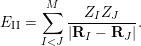
For a given atomic configuration
 $\{\mathbf{R}_{I}\}$
, the ion–ion interaction simply adds a constant shift to the Hamiltonian with
 $$\begin{eqnarray}E_{\text{II}}=\mathop{\sum }_{I<J}^{M}\displaystyle \frac{Z_{I}Z_{J}}{|\mathbf{R}_{I}-\mathbf{R}_{J}|}.\end{eqnarray}$$
We remark that the treatment of periodic systems (more specifically, with a
 $\unicode[STIX]{x1D6E4}$
-point only sampling strategy of the Brillouin zone) is very similar to that for isolated systems. Even for isolated charge-neutral systems, periodic boundary conditions are often used, since they give reasonably accurate approximations as long as certain care is taken with the electrostatic energy (Makov and Payne Reference Makov and Payne1995). Periodic boundary conditions are also more natural for certain numerical methods, such as planewave methods, even for molecular systems.
The ground state is often the most important state. This is because the energy gap
 $E_{1}-E_{0}$
for many electron systems is of the order of electron volts (eV), or
 $10^{4}$
Kelvin when the unit of measurement is
 $k_{B}T$
(
 $k_{B}$
is the Boltzmann constant). This is much greater than room temperature (
 $300$
Kelvin). According to the Boltzmann distribution, the probability of the quantum state
 $E_{i}$
being occupied is
 $\text{e}^{-\unicode[STIX]{x1D6FD}E_{i}}/Z$
, where
 $\unicode[STIX]{x1D6FD}$
is the inverse temperature, and
 $Z$
is a normalization factor called the partition function. Hence the ground state is often the dominating state. Even for certain systems where
 $E_{1}-E_{0}$
is small or zero, the ground state can still be very important. This paper focuses on the calculation of the ground-state energy. In the discussion below, we will simply refer to
 $E_{0}$
as
 $E$
for notational simplicity.
Let
 $\mathbf{x}_{i}=(\mathbf{r}_{i},\unicode[STIX]{x1D70E}_{i})$
denote both the spatial and spin degrees of freedom for the
 $i$
th electron (though electrons are indistinguishable quantum particles). The many-body ground-state wavefunction
 $\unicode[STIX]{x1D6F9}(\mathbf{x}_{1},\ldots ,\mathbf{x}_{N})$
is associated with the smallest eigenvalue
 $E$
of the linear eigenvalue problem
 $$\begin{eqnarray}H\unicode[STIX]{x1D6F9}=E\unicode[STIX]{x1D6F9}.\end{eqnarray}$$
Due to the Pauli exclusion principle for the identical electrons,
 $\unicode[STIX]{x1D6F9}$
is a totally anti-symmetric function:
 $$\begin{eqnarray}\unicode[STIX]{x1D6F9}(\mathbf{x}_{1},\ldots ,\mathbf{x}_{i},\ldots ,\mathbf{x}_{j},\ldots ,\mathbf{x}_{N})=-\unicode[STIX]{x1D6F9}(\mathbf{x}_{1},\ldots ,\mathbf{x}_{j},\ldots ,\mathbf{x}_{i},\ldots ,\mathbf{x}_{N}).\end{eqnarray}$$
The Courant–Fisher minimax theorem states that eigenvalue problem (2.2) can also be viewed as an optimization problem,
 $$\begin{eqnarray}E=\inf _{|\unicode[STIX]{x1D6F9}\rangle \in {\mathcal{A}}_{N},\langle \unicode[STIX]{x1D6F9}|\unicode[STIX]{x1D6F9}\rangle =1}\langle \unicode[STIX]{x1D6F9}|H|\unicode[STIX]{x1D6F9}\rangle ,\end{eqnarray}$$
where
 ${\mathcal{A}}_{N}$
is the set of totally anti-symmetric functions. Equation (2.4) is the variational principle for the ground state in quantum mechanics. Here
 $$\begin{eqnarray}\langle \unicode[STIX]{x1D6F9}|\unicode[STIX]{x1D6F9}\rangle :=\int \unicode[STIX]{x1D6F9}^{\ast }(\mathbf{x}_{1},\ldots ,\mathbf{x}_{N})\unicode[STIX]{x1D6F9}(\mathbf{x}_{1},\ldots ,\mathbf{x}_{N})\,\text{d}\mathbf{x}_{1}\cdots \mathbf{x}_{N}=1\end{eqnarray}$$
defines the normalization condition for the many-body wavefunction, and the integration with respect to a multi-index
 $\mathbf{x}$
should be interpreted as
 $$\begin{eqnarray}\int f(\mathbf{x})\,\text{d}\mathbf{x}:=\mathop{\sum }_{\unicode[STIX]{x1D70E}\in \{\uparrow ,\downarrow \}}\int _{\mathbb{R}^{3}}f(\mathbf{r},\unicode[STIX]{x1D70E})\,\text{d}\mathbf{r}.\end{eqnarray}$$
In order to solve the quantum many-body problem, it appears at first sight that one has to know the quantum many-body wavefunction. Surprisingly, this is at least formally not the case if we are only interested in the ground state. First established by Hohenberg and Kohn (Reference Hohenberg and Kohn1964), density functional theory (DFT) discovered that the many-body electron density, defined by
 $$\begin{eqnarray}\unicode[STIX]{x1D70C}(\mathbf{r})=N\mathop{\sum }_{\unicode[STIX]{x1D70E}\in \{\uparrow ,\downarrow \}}\int |\unicode[STIX]{x1D6F9}((\mathbf{r},\unicode[STIX]{x1D70E}),\mathbf{x}_{2},\ldots ,\mathbf{x}_{n})|^{2}\,\text{d}\mathbf{x}_{2}\cdots \,\text{d}\mathbf{x}_{N},\end{eqnarray}$$
is all one needs to determine the quantum many-body ground state. More specifically, assuming the ground state is non-degenerate, there is a one-to-one correspondence between the electron density
 $\unicode[STIX]{x1D70C}$
and the external potential
 $V_{\text{ext}}$
, so that knowledge of
 $\unicode[STIX]{x1D70C}$
is sufficient to reconstruct the many-body wavefunction
 $\unicode[STIX]{x1D6F9}$
. Shortly thereafter, Mermin (Reference Mermin1965) proposed the DFT formulation in the finite temperature set-up to include thermal effects as well. The most widely used form of DFT, called Kohn–Sham DFT, was proposed by Kohn and Sham (Reference Kohn and Sham1965). Below we introduce DFT from the perspective of constrained minimization, which was first proposed by Levy (Reference Levy1979) and then rigorously established by Lieb (Reference Lieb1983). We also remark that there is as yet no analogous mathematically rigorous theory of DFT for excited states.
2.2 Kohn–Sham density functional theory
According to the variational principle (2.4), the ground-state energy can be written as a constrained minimization problem:
 $$\begin{eqnarray}E=\inf _{\unicode[STIX]{x1D6F9}\in {\mathcal{A}}_{N},\langle \unicode[STIX]{x1D6F9}|\unicode[STIX]{x1D6F9}\rangle =1}\langle \unicode[STIX]{x1D6F9}|H|\unicode[STIX]{x1D6F9}\rangle =\inf _{\unicode[STIX]{x1D70C}\in {\mathcal{J}}_{N}}\Bigg\{\inf _{\substack{ \unicode[STIX]{x1D6F9}\in {\mathcal{A}}_{N} \\ \unicode[STIX]{x1D6F9}\mapsto \unicode[STIX]{x1D70C}}}\langle \unicode[STIX]{x1D6F9}|H|\unicode[STIX]{x1D6F9}\rangle \Bigg\}.\end{eqnarray}$$
Here, on the right-hand side, a constrained minimization given the density
 $\unicode[STIX]{x1D70C}$
is first carried out for the wavefunction
 $\unicode[STIX]{x1D6F9}$
. The resulting value is then optimized as a functional of
 $\unicode[STIX]{x1D70C}$
within the function space
 $$\begin{eqnarray}\displaystyle {\mathcal{J}}_{N}=\bigg\{\unicode[STIX]{x1D70C}\geq 0\;:\;\int \unicode[STIX]{x1D70C}(\mathbf{r})\,\text{d}\mathbf{r}=N,\quad \unicode[STIX]{x1D6FB}\sqrt{\unicode[STIX]{x1D70C}}\in L^{2}(\mathbb{R}^{3})\bigg\}. & & \displaystyle\end{eqnarray}$$
Here the condition
 $\unicode[STIX]{x1D6FB}\sqrt{\unicode[STIX]{x1D70C}}\in L^{2}(\mathbb{R}^{3})$
is implied by the finiteness of the kinetic energy, since
 $$\begin{eqnarray}\displaystyle \displaystyle \frac{1}{2}\int |\unicode[STIX]{x1D6FB}\sqrt{\unicode[STIX]{x1D70C}}(\mathbf{r})|^{2}\,\text{d}\mathbf{r} & \leq & \displaystyle \displaystyle \frac{N}{2}\mathop{\sum }_{\unicode[STIX]{x1D70E}\in \{\uparrow ,\downarrow \}}\int |\unicode[STIX]{x1D6FB}_{\mathbf{r}}\unicode[STIX]{x1D6F9}((\mathbf{r},\unicode[STIX]{x1D70E}),\mathbf{x}_{2},\ldots ,\mathbf{x}_{n})|^{2}\,\text{d}\mathbf{x}_{1}\cdots \,\text{d}\mathbf{x}_{N}\nonumber\\ \displaystyle & = & \displaystyle \langle \unicode[STIX]{x1D6F9}|\hat{T}|\unicode[STIX]{x1D6F9}\rangle .\end{eqnarray}$$
It can also be proved that
 $\unicode[STIX]{x1D70C}\in {\mathcal{J}}_{N}$
implies that there exists at least one
 $\unicode[STIX]{x1D6F9}\in {\mathcal{A}}_{N}$
with finite kinetic energy such that
 $\unicode[STIX]{x1D6F9}\mapsto \unicode[STIX]{x1D70C}$
(Lieb Reference Lieb1983).
Therefore the constrained minimization procedure is well-defined, and we have
 $$\begin{eqnarray}\displaystyle E & = & \displaystyle \inf _{\unicode[STIX]{x1D70C}\in {\mathcal{J}}_{N}}\Bigg\{\inf _{\substack{ \unicode[STIX]{x1D6F9}\in {\mathcal{A}}_{N} \\ \unicode[STIX]{x1D6F9}\mapsto \unicode[STIX]{x1D70C}}}\langle \unicode[STIX]{x1D6F9}|(\hat{T}+\hat{V}_{\text{ee}})|\unicode[STIX]{x1D6F9}\rangle +\int \unicode[STIX]{x1D70C}(\mathbf{r})V_{\text{ext}}(\mathbf{r})\,\text{d}\mathbf{r}\Bigg\}+E_{\text{II}}\end{eqnarray}$$
 $$\begin{eqnarray}\displaystyle & = & \displaystyle \inf _{\unicode[STIX]{x1D70C}\in {\mathcal{J}}_{N}}\bigg\{{\mathcal{F}}_{\text{LL}}[\unicode[STIX]{x1D70C}]+\int \unicode[STIX]{x1D70C}(\mathbf{r})V_{\text{ext}}(\mathbf{r})\,\text{d}\mathbf{r}\bigg\}+E_{\text{II}}.\end{eqnarray}$$
Here, together with equation (2.7), we have used
 $$\begin{eqnarray}\displaystyle \langle \unicode[STIX]{x1D6F9}|\hat{V}_{\text{ext}}|\unicode[STIX]{x1D6F9}\rangle =N\int |\unicode[STIX]{x1D6F9}(\mathbf{x}_{1},\ldots ,\mathbf{x}_{N})|^{2}V_{\text{ext}}(\mathbf{r}_{1})\,\text{d}\mathbf{x}_{1}\cdots \,\text{d}\mathbf{x}_{N}=\int \unicode[STIX]{x1D70C}(\mathbf{r})V_{\text{ext}}(\mathbf{r})\,\text{d}\mathbf{r}. & & \displaystyle\end{eqnarray}$$
The functional
 ${\mathcal{F}}_{\text{LL}}[\unicode[STIX]{x1D70C}]$
is universal, since it depends only on the kinetic and electron–electron repulsion but not on the external potential
 $V_{\text{ext}}$
, which is specified by the atomic configuration. Another important consequence of density functional theory, often known as the Hohenberg–Kohn theorem (Hohenberg and Kohn Reference Hohenberg and Kohn1964), is that if
 $\unicode[STIX]{x1D70C}^{\star }$
is the minimizer of (2.12) and if
 $\unicode[STIX]{x1D6F9}^{\star }$
is the unique minimizer that results in
 ${\mathcal{F}}_{\text{LL}}[\unicode[STIX]{x1D70C}^{\star }]$
, then the many-body ground-state wavefunction
 $\unicode[STIX]{x1D6F9}^{\star }$
is determined by the electron density
 $\unicode[STIX]{x1D70C}^{\star }$
. In other words, if the ground state is non-degenerate, then there is a one-to-one mapping between the ground-state electron density and the many-body ground-state wavefunction. All that remains to make DFT useful is thus a good explicit expression that approximates the functional
 ${\mathcal{F}}_{\text{LL}}[\unicode[STIX]{x1D70C}]$
.
Since the very early days of quantum mechanics, physicists have been seeking the approximation to
 ${\mathcal{F}}_{\text{LL}}[\unicode[STIX]{x1D70C}]$
(before it was connected to density functional theory) pioneered by Thomas (Reference Thomas1927) and Fermi (Reference Fermi1927). Until the 1960s, efforts were mainly restricted to uniform electron gas, that is, the system is in a periodic box with a constant external potential field, where many calculations can be done analytically. Despite significant progress in the past few decades, modelling
 ${\mathcal{F}}_{\text{LL}}[\unicode[STIX]{x1D70C}]$
remains a very difficult task. To appreciate the difficulty, just recall the atomic shell structure from the eigenfunctions of the Hamiltonian operator of a hydrogen atom. It is already highly non-trivial to find such a mapping for a single atom. Furthermore, in chemistry and materials science, the absolute value of the energy is usually not the most important quantity. It is the relative energy difference that determines whether or not a chemical process should occur. This often requires the ground-state energy to be calculated with
 $99.9\%$
accuracy or higher.
The breakthrough of density functional theory is generally attributed to Kohn and Sham (Reference Kohn and Sham1965), who proposed combining DFT with single-particle orbital structure. Given
 $N$
one-particle orthonormal spin-orbitals
 $\{\unicode[STIX]{x1D713}_{i}(\mathbf{x})\}_{i=1}^{N}$
, that is,
 $$\begin{eqnarray}\langle \unicode[STIX]{x1D713}_{i}|\unicode[STIX]{x1D713}_{j}\rangle :=\int \unicode[STIX]{x1D713}_{i}^{\ast }(\mathbf{x})\unicode[STIX]{x1D713}_{j}(\mathbf{x})\,\text{d}\mathbf{x}=\unicode[STIX]{x1D6FF}_{ij},\quad i,j=1,\ldots ,N,\end{eqnarray}$$
the associated Slater determinant is given by
 $$\begin{eqnarray}\unicode[STIX]{x1D6F9}(\mathbf{x}_{1},\ldots ,\mathbf{x}_{N})=\displaystyle \frac{1}{\sqrt{N!}}\det \left(\begin{array}{@{}cccc@{}}\unicode[STIX]{x1D713}_{1}(\mathbf{x}_{1}) & \unicode[STIX]{x1D713}_{1}(\mathbf{x}_{2}) & \cdots \, & \unicode[STIX]{x1D713}_{1}(\mathbf{x}_{N})\\ \unicode[STIX]{x1D713}_{2}(\mathbf{x}_{1}) & \unicode[STIX]{x1D713}_{2}(\mathbf{x}_{2}) & \cdots \, & \unicode[STIX]{x1D713}_{2}(\mathbf{x}_{N})\\ \vdots & \vdots & \ddots & \vdots \\ \unicode[STIX]{x1D713}_{N}(\mathbf{x}_{1}) & \unicode[STIX]{x1D713}_{N}(\mathbf{x}_{2}) & \cdots \, & \unicode[STIX]{x1D713}_{N}(\mathbf{x}_{N})\end{array}\right)\!,\end{eqnarray}$$
which is anti-symmetric by the property of determinants. The computation of the electron density (2.7) with respect to a Slater determinant can be simplified as
 $$\begin{eqnarray}\unicode[STIX]{x1D70C}(\mathbf{r})=\mathop{\sum }_{i=1}^{N}\mathop{\sum }_{\unicode[STIX]{x1D70E}\in \{\uparrow ,\downarrow \}}|\unicode[STIX]{x1D713}_{i}(\mathbf{r},\unicode[STIX]{x1D70E})|^{2}.\end{eqnarray}$$
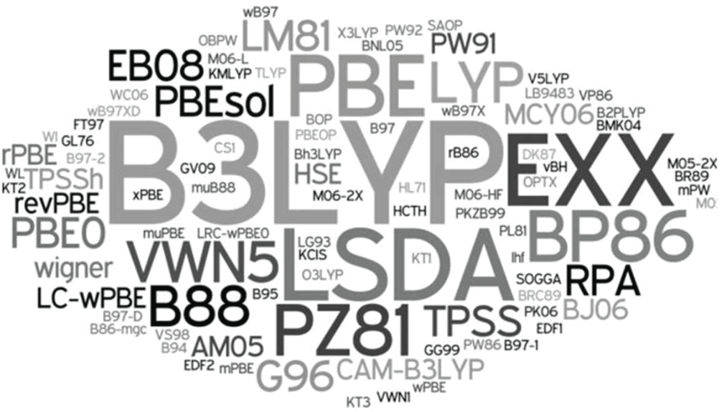
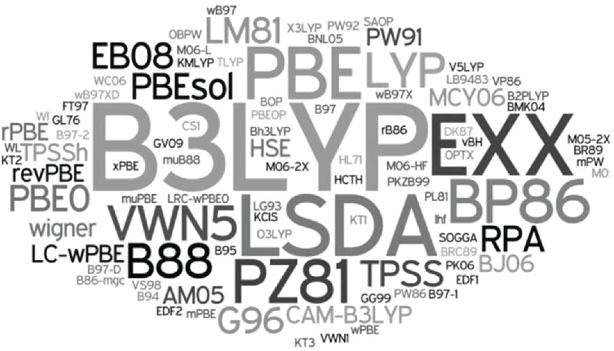
(Credit: Burke Reference Burke2012.) A ‘zoo’ of exchange-correlation functionals in DFT.
Using constrained minimization over Slater determinants, the Kohn–Sham proposal can be interpreted as
 $$\begin{eqnarray}{\mathcal{F}}_{\text{LL}}[\unicode[STIX]{x1D70C}]=\inf _{\substack{ \unicode[STIX]{x1D6F9}\in {\mathcal{A}}_{N}^{0} \\ \unicode[STIX]{x1D6F9}\mapsto \unicode[STIX]{x1D70C}}}\langle \unicode[STIX]{x1D6F9}|\hat{T}|\unicode[STIX]{x1D6F9}\rangle +\displaystyle \frac{1}{2}\int \displaystyle \frac{\unicode[STIX]{x1D70C}(\mathbf{r})\unicode[STIX]{x1D70C}(\mathbf{r}^{\prime })}{|\mathbf{r}-\mathbf{r}^{\prime }|}\,\text{d}\mathbf{r}\,\text{d}\mathbf{r}^{\prime }+E_{\text{xc}}[\unicode[STIX]{x1D70C}],\end{eqnarray}$$
where
 ${\mathcal{A}}_{N}^{0}$
is the set of Slater determinants with
 $N$
orbitals. It turns out that for any
 $\unicode[STIX]{x1D70C}\in {\mathcal{J}}_{N}$
there exists at least one
 $\unicode[STIX]{x1D6F9}\in {\mathcal{A}}_{N}^{0}$
that gives the density
 $\unicode[STIX]{x1D70C}$
, and the constrained minimization of the kinetic energy term is well-defined (Lieb Reference Lieb1983). In equation (2.17), the first term corresponds to the kinetic energy from
 $N$
non-interacting single-particle orbitals. The second term is the Hartree energy, which characterizes the electron–electron repulsion energy at the mean-field level. The last term
 $E_{\text{xc}}[\unicode[STIX]{x1D70C}]$
, called the exchange-correlation functional, at first glance simply defines whatever we do not know about
 ${\mathcal{F}}_{\text{LL}}[\unicode[STIX]{x1D70C}]$
. The insight from Kohn and Sham (Reference Kohn and Sham1965) is that the kinetic and Hartree terms often account for more than
 $95\%$
of the total energy. Therefore the approximation to
 $E_{\text{xc}}[\unicode[STIX]{x1D70C}]$
, while still very difficult, is a much easier task than approximating
 ${\mathcal{F}}_{\text{LL}}[\unicode[STIX]{x1D70C}]$
directly. As a result, the approximation to the ground-state energy in the Kohn–Sham DFT is given by minimizing over the Kohn–Sham energy functional:
 $$\begin{eqnarray}\displaystyle E^{\text{KS}} & = & \displaystyle \inf _{\unicode[STIX]{x1D6F9}\in {\mathcal{A}}_{N}^{0}}\bigg\{\langle \unicode[STIX]{x1D6F9}|\hat{T}|\unicode[STIX]{x1D6F9}\rangle +\displaystyle \frac{1}{2}\int \displaystyle \frac{\unicode[STIX]{x1D70C}(\mathbf{r})\unicode[STIX]{x1D70C}(\mathbf{r}^{\prime })}{|\mathbf{r}-\mathbf{r}^{\prime }|}\,\text{d}\mathbf{r}\,\text{d}\mathbf{r}^{\prime }\nonumber\\ \displaystyle & & \displaystyle \qquad \qquad +E_{\text{xc}}[\unicode[STIX]{x1D70C}]+\int \unicode[STIX]{x1D70C}(\mathbf{r})V_{\text{ext}}(\mathbf{r})\,\text{d}\mathbf{r}\bigg\}+E_{\text{II}},\end{eqnarray}$$
with
 $\unicode[STIX]{x1D70C}$
given by the Slater determinant
 $\unicode[STIX]{x1D6F9}$
. Writing the kinetic energy of the Slater determinant more explicitly, we have
 $$\begin{eqnarray}E^{\text{KS}}=\inf _{\{\unicode[STIX]{x1D713}_{i}\}_{i=1}^{N},\langle \unicode[STIX]{x1D713}_{i}|\unicode[STIX]{x1D713}_{j}\rangle =\unicode[STIX]{x1D6FF}_{ij}}{\mathcal{F}}^{\text{KS}}(\{\unicode[STIX]{x1D713}_{i}\})+E_{\text{II}}\end{eqnarray}$$
with
 $$\begin{eqnarray}\displaystyle {\mathcal{F}}^{\text{KS}}(\{\unicode[STIX]{x1D713}_{i}\}) & = & \displaystyle \displaystyle \frac{1}{2}\mathop{\sum }_{i=1}^{N}\int |\unicode[STIX]{x1D6FB}_{\mathbf{r}}\unicode[STIX]{x1D713}_{i}(\mathbf{x})|^{2}\,\text{d}\mathbf{x}+\int \unicode[STIX]{x1D70C}(\mathbf{r})V_{\text{ext}}(\mathbf{r})\,\text{d}\mathbf{r}\nonumber\\ \displaystyle & & \displaystyle \qquad +\,\displaystyle \frac{1}{2}\int \displaystyle \frac{\unicode[STIX]{x1D70C}(\mathbf{r})\unicode[STIX]{x1D70C}(\mathbf{r}^{\prime })}{|\mathbf{r}-\mathbf{r}^{\prime }|}\,\text{d}\mathbf{r}\,\text{d}\mathbf{r}^{\prime }+E_{\text{xc}}[\unicode[STIX]{x1D70C}].\end{eqnarray}$$
The Kohn–Sham DFT would in principle be exact if we had access to the exact exchange-correlation functional
 $E_{\text{xc}}[\unicode[STIX]{x1D70C}]$
. The exchange-correlation functional is also universal, i.e. independent of the external potential
 $V_{\text{ext}}$
and hence the atomic configuration. In order to use Kohn–Sham DFT in practice, the exchange-correlation functional
 $E_{\text{xc}}$
must be approximated. Starting from the local density approximation proposed by Kohn and Sham, a ‘zoo’ of exchange-correlation functionals has been proposed: see an incomplete list in Figure 2.1 by Burke (Reference Burke2012).
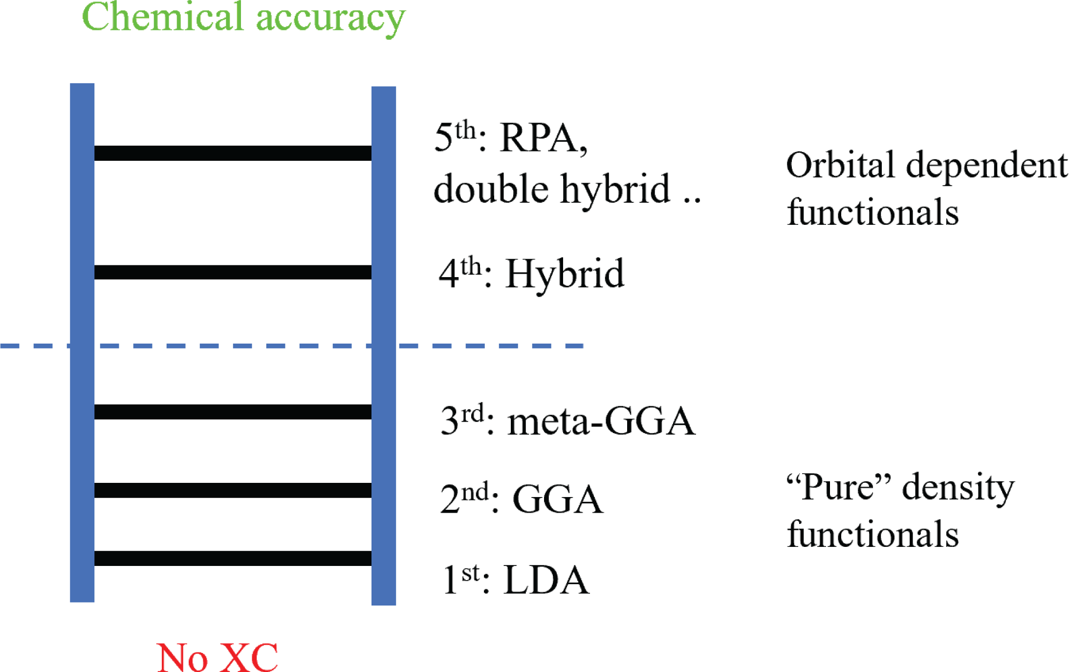
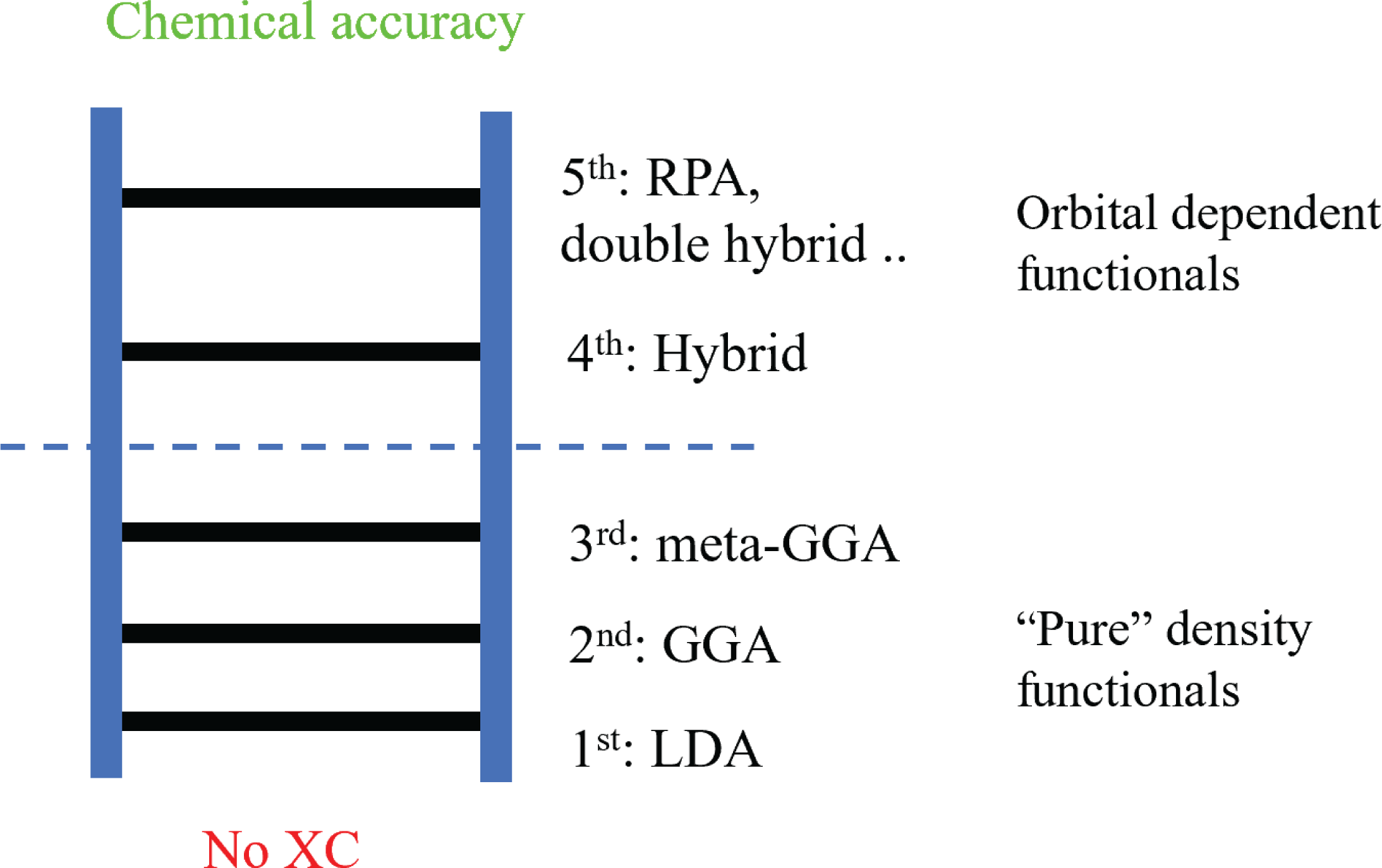
According to Perdew (Perdew and Schmidt Reference Perdew and Schmidt2001, Perdew Reference Perdew2013), these exchange-correlation functionals can be organized using a ‘Jacob’s ladder’ for exchange-correlation functionals (Figure 2.2). When no exchange-correlation functional is used, Kohn–Sham DFT is essentially a Hartree approximation (with Pauli’s exclusion principle). In such a case, DFT is significantly less accurate than Hartree–Fock theory (Szabo and Ostlund Reference Szabo and Ostlund1989), and the latter is often regarded as the starting point of quantum chemistry. This is referred to as ‘Hartree’s hell’. Moving up the ladder, the accuracy of the DFT calculation generally improves towards the ‘heaven of chemical accuracy’ of
 $1$
kcal/mol (or
 $1.6\times 10^{-3}$
Hartree per atom) when compared to experimental results. Correspondingly, the functional forms become increasingly more complex, which leads to higher computational costs.
The ‘Jacob’s ladder’ of exchange-correlation functionals.
On the first rung of the ladder, we have the local density approximation (LDA), where
 $E_{\text{xc}}$
is modelled locally by the electron density
 $$\begin{eqnarray}E_{\text{xc}}[\unicode[STIX]{x1D70C}]=\int \unicode[STIX]{x1D716}_{\text{xc}}(\unicode[STIX]{x1D70C}(\mathbf{r}))\,\text{d}\mathbf{r}.\end{eqnarray}$$
Note that the integrand
 $\unicode[STIX]{x1D716}_{\text{xc}}(\unicode[STIX]{x1D70C}(\mathbf{r}))$
depends only on the electron density at
 $\mathbf{r}$
. The most widely used LDA exchange-correlation functional is obtained by parametrizing the result from the quantum Monte Carlo simulation (QMC) obtained for the uniform electron gas system in the 1980s (Ceperley and Alder Reference Ceperley and Alder1980, Perdew and Zunger Reference Perdew and Zunger1981). Although most, if not all, real chemical and materials systems are very different from the uniform electron gas system, the Kohn–Sham DFT calculations with such LDA exchange-correlation functionals already perform surprisingly well for many systems.
In order to improve the accuracy of the exchange-correlation functional, on the next rung of the ladder we have the generalized gradient approximation (GGA) (Lee et al. Reference Lee, Yang and Parr1988, Becke Reference Becke1988, Perdew et al. Reference Perdew, Burke and Ernzerhof1996a ), which in addition depends on information on the gradient of electron density,
 $$\begin{eqnarray}E_{\text{xc}}[\unicode[STIX]{x1D70C}]=\int \unicode[STIX]{x1D716}_{\text{xc}}(\unicode[STIX]{x1D70C}(\mathbf{r}),\unicode[STIX]{x1D70E}(\mathbf{r}))\,\text{d}\mathbf{r},\end{eqnarray}$$
where the functional depends only on the norm of the gradient
 $$\begin{eqnarray}\unicode[STIX]{x1D70E}(\mathbf{r}):=|\unicode[STIX]{x1D6FB}\unicode[STIX]{x1D70C}(\mathbf{r})|^{2}\end{eqnarray}$$
due to local rotational symmetry. The GGA functionals are currently the most widely used functionals since they achieve a balance between accuracy and computational cost.
The third rung of the ladder is the meta-GGA approximation (Staroverov, Scuseria, Tao and Perdew Reference Staroverov, Scuseria, Tao and Perdew2003, Sun, Ruzsinszky and Perdew Reference Sun, Ruzsinszky and Perdew2015), where second-order derivative information is also added to the approximation, in particular the kinetic energy density
 $$\begin{eqnarray}\unicode[STIX]{x1D70F}(\mathbf{r}):=\displaystyle \frac{1}{2}\mathop{\sum }_{\unicode[STIX]{x1D70E}\in \{\uparrow ,\downarrow \}}\mathop{\sum }_{i=1}^{N}|\unicode[STIX]{x1D6FB}_{\boldsymbol{ r}}\unicode[STIX]{x1D713}_{i}(\mathbf{r},\unicode[STIX]{x1D70E})|^{2}.\end{eqnarray}$$
The meta-GGA energy functional then takes the form
 $$\begin{eqnarray}E_{\text{xc}}[\{\unicode[STIX]{x1D713}_{i}\}]=\int \unicode[STIX]{x1D716}_{\text{xc}}(\unicode[STIX]{x1D70C}(\mathbf{r}),\unicode[STIX]{x1D70E}(\mathbf{r}),\unicode[STIX]{x1D70F}(\mathbf{r}))\,\text{d}\mathbf{r}.\end{eqnarray}$$
Some other meta-GGA functionals also involve second-order information on the density, i.e.
 $\unicode[STIX]{x1D6FB}^{2}\unicode[STIX]{x1D70C}(\mathbf{r})$
, and for simplicity we omit treatment of such terms. Since
 $\unicode[STIX]{x1D70F}$
is the local kinetic energy of the orbitals, it may seem that the meta-GGA functional is no longer strictly a density functional. It turns out that the Euler–Lagrange equation associated with the meta-GGA functional can still be written in the same form as that of the LDA and GGA energy functionals, as we will see in the next section. Hence, the LDA, GGA and meta-GGA functionals are known as semi-local functionals, and their numerical treatment is very similar, as will be discussed in Section 5.
Let us remark that the exchange-correlation functionals discussed so far do not explicitly depend on spin degrees of freedom (i.e. they are only functionals of the electron density rather than the spin-dependent electron density). Spin-dependent exchange-correlation functionals, such as local-spin-density approximation (LSDA) (von Barth and Hedin Reference von Barth and Hedin1972), are developed for spin-polarized systems. From the perspective of numerical algorithms they are rather similar to the exchange-correlation functionals without spin dependence, so we will not go into the details.
The exchange-correlation functionals beyond the third rung are called non-local functionals, and will be discussed in Section 2.5. Before diving into these more complicated exchange-correlation functionals, we first introduce the Kohn–Sham equations, i.e. the Euler–Lagrange equation for Kohn–Sham density functional theory.
2.3 Kohn–Sham equations for semi-local functionals
In order to minimize the Kohn–Sham energy functional (2.20), we need to find the stationary point of the Lagrangian. Let us consider the case of the LDA exchange-correlation functional first. Note that
 $$\begin{eqnarray}\displaystyle \frac{1}{2}{\displaystyle \frac{\unicode[STIX]{x1D6FF}{\mathcal{F}}^{\text{KS}}(\{\unicode[STIX]{x1D713}_{i}\})}{\unicode[STIX]{x1D6FF}\unicode[STIX]{x1D713}_{i}^{\ast }(\mathbf{x})}}=\biggl(-\displaystyle \frac{1}{2}\unicode[STIX]{x1D6E5}_{\mathbf{r}}+V_{\text{ext}}+V_{H}[\unicode[STIX]{x1D70C}]+V_{\text{xc}}[\unicode[STIX]{x1D70C}]\biggr)\unicode[STIX]{x1D713}_{i}(\mathbf{x})=:H^{\text{KS}}[\unicode[STIX]{x1D70C}]\unicode[STIX]{x1D713}_{i}(\mathbf{x}),\end{eqnarray}$$
where the effective Kohn–Sham Hamiltonian
 $H^{\text{KS}}[\unicode[STIX]{x1D70C}]$
is an operator acting on the orbitals which depends on
 $\unicode[STIX]{x1D70C}$
, given by the orbitals as in equation (2.16). The Hartree potential
 $V_{H}$
is given by the Coulomb kernel via
 $$\begin{eqnarray}V_{H}[\unicode[STIX]{x1D70C}](\mathbf{r})=(v_{C}\unicode[STIX]{x1D70C})(\mathbf{r}):=\int {\displaystyle \frac{\unicode[STIX]{x1D70C}(\mathbf{r}^{\prime })}{|\mathbf{r}-\mathbf{r}^{\prime }|}}\,\text{d}\mathbf{r}^{\prime },\end{eqnarray}$$
and the exchange-correlation potential is defined to be the functional derivative of
 $E_{\text{xc}}$
, that is,
 $$\begin{eqnarray}\displaystyle V_{\text{xc}}[\unicode[STIX]{x1D70C}]=\displaystyle \frac{\unicode[STIX]{x1D6FF}E_{\text{xc}}[\unicode[STIX]{x1D70C}]}{\unicode[STIX]{x1D6FF}\unicode[STIX]{x1D70C}}, & & \displaystyle\end{eqnarray}$$
which for now can be thought of as a
 $\unicode[STIX]{x1D70C}$
-dependent potential acting on orbitals.
 $V_{\text{xc}}$
of more general forms will be discussed further and made more explicit at the end of this section.
Taking into account the orthonormality condition (2.14), we obtain the Euler–Lagrange equations
 $$\begin{eqnarray}\displaystyle H^{\text{KS}}[\unicode[STIX]{x1D70C}]\unicode[STIX]{x1D713}_{i}(\mathbf{x})=\biggl(-\displaystyle \frac{1}{2}\unicode[STIX]{x1D6E5}_{\mathbf{r}}+V_{\text{ext}}+V_{H}[\unicode[STIX]{x1D70C}]+V_{\text{xc}}[\unicode[STIX]{x1D70C}]\biggr)\unicode[STIX]{x1D713}_{i}(\mathbf{x})=\mathop{\sum }_{j=1}^{N}\unicode[STIX]{x1D713}_{j}(\mathbf{x})\unicode[STIX]{x1D706}_{ij}, & & \displaystyle\end{eqnarray}$$
where the
 $\unicode[STIX]{x1D706}_{ij}$
are Lagrange multipliers. Let us further simplify the Euler–Lagrange equations to reveal the structure of the problem. First note that due to the orthonormality of
 $\{\unicode[STIX]{x1D713}_{i}\}$
and the self-adjointness of
 $H^{\text{KS}}[\unicode[STIX]{x1D70C}]$
, we have
 $$\begin{eqnarray}\unicode[STIX]{x1D706}_{ij}=\langle \unicode[STIX]{x1D713}_{j}|H^{\text{KS}}[\unicode[STIX]{x1D70C}]|\unicode[STIX]{x1D713}_{i}\rangle =\langle \unicode[STIX]{x1D713}_{i}|H^{\text{KS}}[\unicode[STIX]{x1D70C}]|\unicode[STIX]{x1D713}_{j}\rangle ^{\ast }=\unicode[STIX]{x1D706}_{ji}^{\ast }.\end{eqnarray}$$
Therefore
 $\unicode[STIX]{x1D6EC}=(\unicode[STIX]{x1D706}_{ij})$
is a Hermitian matrix, and we may assume an eigen-decomposition of
 $\unicode[STIX]{x1D6EC}$
as
 $$\begin{eqnarray}\unicode[STIX]{x1D6EC}=U\operatorname{diag}(\unicode[STIX]{x1D700}_{1},\ldots ,\unicode[STIX]{x1D700}_{n})U^{\ast },\end{eqnarray}$$
where
 $U$
is a unitary matrix.
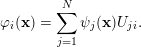
Now consider a rotation of the orbitals, that is,
 $$\begin{eqnarray}\unicode[STIX]{x1D711}_{i}(\mathbf{x})=\mathop{\sum }_{j=1}^{N}\unicode[STIX]{x1D713}_{j}(\mathbf{x})U_{ji}.\end{eqnarray}$$
Since
 $U$
is a unitary matrix, the transformation preserves the electron density and hence the effective Kohn–Sham Hamiltonian. The equations for the rotated orbitals
 $\{\unicode[STIX]{x1D711}_{i}\}$
become
 $$\begin{eqnarray}\displaystyle H^{\text{KS}}[\unicode[STIX]{x1D70C}]\unicode[STIX]{x1D711}_{i}(\mathbf{x}) & = & \displaystyle H^{\text{KS}}[\unicode[STIX]{x1D70C}]\mathop{\sum }_{j=1}^{N}\unicode[STIX]{x1D713}_{j}(\mathbf{x})U_{ji}=\mathop{\sum }_{k,j=1}^{N}\unicode[STIX]{x1D713}_{k}(\mathbf{x})\unicode[STIX]{x1D706}_{kj}U_{ji}\nonumber\\ \displaystyle & = & \displaystyle \mathop{\sum }_{k=1}^{N}\unicode[STIX]{x1D713}_{k}(\mathbf{x})U_{ki}\unicode[STIX]{x1D700}_{i}=\unicode[STIX]{x1D711}_{i}(\mathbf{x})\unicode[STIX]{x1D700}_{i}.\end{eqnarray}$$
Therefore, without loss of generality (up to a rotation of orbitals), it suffices to consider the Euler–Lagrange equations of the form
 $$\begin{eqnarray}\displaystyle \biggl(-\displaystyle \frac{1}{2}\unicode[STIX]{x1D6E5}_{\mathbf{r}}+V_{\text{ext}}+V_{H}[\unicode[STIX]{x1D70C}]+V_{\text{xc}}[\unicode[STIX]{x1D70C}]\biggr)\unicode[STIX]{x1D713}_{i}(\mathbf{x})=\unicode[STIX]{x1D700}_{i}\unicode[STIX]{x1D713}_{i}(\mathbf{x}),\quad i=1,\ldots ,N. & & \displaystyle\end{eqnarray}$$
Since the operator
 $H^{\text{KS}}$
depends on the orbitals
 $\{\unicode[STIX]{x1D713}_{i}\}$
via the electron density
 $\unicode[STIX]{x1D70C}$
, this is a set of nonlinear eigenvalue problems, known as the Kohn–Sham equations. Here the Hamiltonian is nonlinear with respect to the eigenvectors, rather than the eigenvalues.
The Kohn–Sham equations (2.32) must be solved self-consistently with respect to the electron density
 $\unicode[STIX]{x1D70C}$
. For a given electron density
 $\unicode[STIX]{x1D70C}$
, the Hamiltonian
 $H^{\text{KS}}[\unicode[STIX]{x1D70C}]=-{\textstyle \frac{1}{2}}\unicode[STIX]{x1D6E5}_{\mathbf{r}}+V_{\text{eff}}(\mathbf{r})$
is a self-adjoint linear operator, where the effective potential induced by
 $\unicode[STIX]{x1D70C}$
is
 $$\begin{eqnarray}V_{\text{eff}}(\mathbf{r})=V_{\text{ext}}(\mathbf{r})+V_{H}[\unicode[STIX]{x1D70C}](\mathbf{r})+V_{\text{xc}}[\unicode[STIX]{x1D70C}](\mathbf{r}).\end{eqnarray}$$
The Kohn–Sham orbitals
 $\{\unicode[STIX]{x1D713}_{i}\}$
are thus eigenfunctions of
 $H^{\text{KS}}[\unicode[STIX]{x1D70C}]$
. It should be noted that a priori there is no guarantee that
 $\{\unicode[STIX]{x1D713}_{i}\}_{i=1}^{N}$
should correspond to the lowest
 $N$
eigenvalues (counting multiplicity) of
 $H^{\text{KS}}[\unicode[STIX]{x1D70C}]$
to achieve the global minimum of the Kohn–Sham energy functional (2.18). In practice, this is often assumed in solving the Kohn–Sham equations, known as the aufbau principle. It is known that the aufbau principle holds for non-interacting systems, as well as certain Hartree–Fock models. However, it can be violated for more complex models such as Kohn–Sham DFT. Assuming the aufbau principle, the first
 $N$
eigenfunctions
 $\{\unicode[STIX]{x1D713}_{i}\}_{i=1}^{N}$
are called occupied orbitals, while the eigenfunctions of
 $H^{\text{KS}}[\unicode[STIX]{x1D70C}]$
with higher eigenvalues are called virtual or unoccupied orbitals.
For Kohn–Sham DFT with semi-local exchange-correlation functionals, the effective Kohn–Sham potential
 $V_{\text{eff}}[\unicode[STIX]{x1D70C}]$
, and hence the Hamiltonian matrix, depends only on the density
 $\unicode[STIX]{x1D70C}$
through the Kohn–Sham potential. We refer to the mapping from
 $V_{\text{eff}}$
to
 $\unicode[STIX]{x1D70C}$
as the Kohn–Sham map, denoted by
 $$\begin{eqnarray}\unicode[STIX]{x1D70C}={\mathcal{F}}_{\text{KS}}[V_{\text{eff}}].\end{eqnarray}$$
The electron density
 $\unicode[STIX]{x1D70C}$
can be evaluated from the Kohn–Sham map by solving a linear eigenvalue problem, or using density matrix techniques, to be discussed in Section 5. Hence
 $\unicode[STIX]{x1D70C}$
and
 $V_{\text{eff}}$
should be iteratively determined by each other until convergence. This is called the self-consistent field (SCF) iteration.
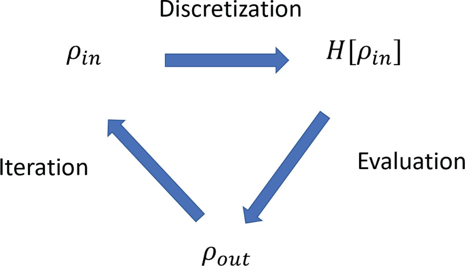
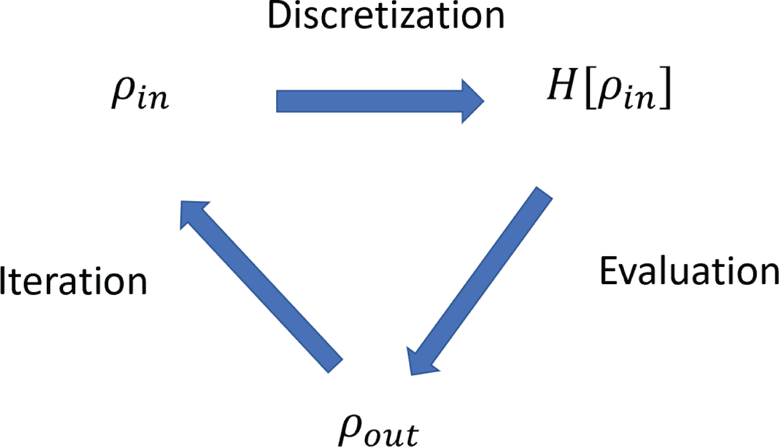
The numerical solution for solving the Kohn–Sham equations can thus be divided into three subproblems, as illustrated in Figure 2.3: discretization of the Kohn–Sham Hamiltonian using a finite basis set, evaluation of the Kohn–Sham map, and iteration until reaching self-consistency. The content of this review is thus largely organized around these three topics. Note that during the self-consistent iteration, one also needs to form the Kohn–Sham Hamiltonian by evaluating the Hartree and exchange-correlation potential. With some abuse of terminology, we consider this step as part of the discretization problem in Figure 2.3. We remark that the evaluation of the Hartree potential requires solving a Poisson equation. Depending on the choice of the basis set, the solution can be efficiently obtained using the fast Fourier transform or multigrid methods (see e.g. Brandt Reference Brandt1977, Brandt, McCormick and Ruge Reference Brandt, McCormick and Ruge1985, Briggs, Henson and McCormick Reference Briggs, Henson and McCormick2000, Fattebert and Bernholc Reference Fattebert and Bernholc2000).
Three subproblems for the self-consistent solution of the Kohn–Sham equations. With some abuse of terminology, the step of forming the Kohn–Sham Hamiltonian is considered to be part of the discretization step in this figure.
Let us now come back to the exchange-correlation potential, given by the functional derivative of
 $E_{\text{xc}}$
with respect to the density. For LDA, the variation of
 $E_{\text{xc}}$
is given by
 $$\begin{eqnarray}\unicode[STIX]{x1D6FF}E_{\text{xc}}=\int \displaystyle \frac{\unicode[STIX]{x2202}\unicode[STIX]{x1D716}_{\text{xc}}}{\unicode[STIX]{x2202}\unicode[STIX]{x1D70C}}(\unicode[STIX]{x1D70C}(\mathbf{r}))\unicode[STIX]{x1D6FF}\unicode[STIX]{x1D70C}(\mathbf{r})\,\text{d}\mathbf{r}.\end{eqnarray}$$
Hence
 $$\begin{eqnarray}V_{\text{xc}}[\unicode[STIX]{x1D70C}](\mathbf{r})=\displaystyle \frac{\unicode[STIX]{x1D6FF}E_{\text{xc}}}{\unicode[STIX]{x1D6FF}\unicode[STIX]{x1D70C}(\mathbf{r})}=\displaystyle \frac{\unicode[STIX]{x2202}\unicode[STIX]{x1D716}_{\text{xc}}}{\unicode[STIX]{x2202}\unicode[STIX]{x1D70C}}(\unicode[STIX]{x1D70C}(\mathbf{r})).\end{eqnarray}$$
For GGA, the variation with respect to the density gives
 $$\begin{eqnarray}\unicode[STIX]{x1D6FF}E_{\text{xc}}=\int \displaystyle \frac{\unicode[STIX]{x2202}\unicode[STIX]{x1D716}_{\text{xc}}}{\unicode[STIX]{x2202}\unicode[STIX]{x1D70C}}\unicode[STIX]{x1D6FF}\unicode[STIX]{x1D70C}+\displaystyle \frac{\unicode[STIX]{x2202}\unicode[STIX]{x1D716}_{\text{xc}}}{\unicode[STIX]{x2202}\unicode[STIX]{x1D70E}}\unicode[STIX]{x1D6FF}\unicode[STIX]{x1D70E}\,\text{d}\mathbf{r}.\end{eqnarray}$$
Using the chain rule,
 $$\begin{eqnarray}\unicode[STIX]{x1D6FF}\unicode[STIX]{x1D70E}=|\unicode[STIX]{x1D6FB}(\unicode[STIX]{x1D70C}+\unicode[STIX]{x1D6FF}\unicode[STIX]{x1D70C})|^{2}-|\unicode[STIX]{x1D6FB}\unicode[STIX]{x1D70C}|^{2}=2\unicode[STIX]{x1D6FB}\unicode[STIX]{x1D70C}\cdot \unicode[STIX]{x1D6FB}\unicode[STIX]{x1D6FF}\unicode[STIX]{x1D70C}+O(|\unicode[STIX]{x1D6FF}\unicode[STIX]{x1D70C}|^{2}),\end{eqnarray}$$
we have
 $$\begin{eqnarray}\unicode[STIX]{x1D6FF}E_{\text{xc}}=\int \displaystyle \frac{\unicode[STIX]{x2202}\unicode[STIX]{x1D716}_{\text{xc}}}{\unicode[STIX]{x2202}\unicode[STIX]{x1D70C}}\unicode[STIX]{x1D6FF}\unicode[STIX]{x1D70C}+2\displaystyle \frac{\unicode[STIX]{x2202}\unicode[STIX]{x1D716}_{\text{xc}}}{\unicode[STIX]{x2202}\unicode[STIX]{x1D70E}}(\unicode[STIX]{x1D6FB}\unicode[STIX]{x1D70C}\cdot \unicode[STIX]{x1D6FB}\unicode[STIX]{x1D6FF}\unicode[STIX]{x1D70C})\,\text{d}\mathbf{r}=\int \displaystyle \frac{\unicode[STIX]{x2202}\unicode[STIX]{x1D716}_{\text{xc}}}{\unicode[STIX]{x2202}\unicode[STIX]{x1D70C}}\unicode[STIX]{x1D6FF}\unicode[STIX]{x1D70C}-2\unicode[STIX]{x1D6FB}\cdot \biggl(\displaystyle \frac{\unicode[STIX]{x2202}\unicode[STIX]{x1D716}_{\text{xc}}}{\unicode[STIX]{x2202}\unicode[STIX]{x1D70E}}\unicode[STIX]{x1D6FB}\unicode[STIX]{x1D70C}\biggr)\unicode[STIX]{x1D6FF}\unicode[STIX]{x1D70C}\,\text{d}\mathbf{r}.\end{eqnarray}$$
Thus
 $$\begin{eqnarray}V_{\text{xc}}[\unicode[STIX]{x1D70C}]=\displaystyle \frac{\unicode[STIX]{x2202}\unicode[STIX]{x1D716}_{\text{xc}}}{\unicode[STIX]{x2202}\unicode[STIX]{x1D70C}}-2\unicode[STIX]{x1D6FB}\cdot \biggl(\displaystyle \frac{\unicode[STIX]{x2202}\unicode[STIX]{x1D716}_{\text{xc}}}{\unicode[STIX]{x2202}\unicode[STIX]{x1D70E}}\unicode[STIX]{x1D6FB}\unicode[STIX]{x1D70C}\biggr).\end{eqnarray}$$
The derivation of the exchange-correlation potential is slightly different for meta-GGA, since the kinetic energy density
 $\unicode[STIX]{x1D70F}(\mathbf{r})$
explicitly involves the Kohn–Sham orbitals
 $\{\unicode[STIX]{x1D713}_{i}\}$
. We still start with
 $$\begin{eqnarray}\unicode[STIX]{x1D6FF}E_{\text{xc}}=\int \displaystyle \frac{\unicode[STIX]{x2202}\unicode[STIX]{x1D716}_{\text{xc}}}{\unicode[STIX]{x2202}\unicode[STIX]{x1D70C}}\unicode[STIX]{x1D6FF}\unicode[STIX]{x1D70C}+\displaystyle \frac{\unicode[STIX]{x2202}\unicode[STIX]{x1D716}_{\text{xc}}}{\unicode[STIX]{x2202}\unicode[STIX]{x1D70E}}\unicode[STIX]{x1D6FF}\unicode[STIX]{x1D70E}+\displaystyle \frac{\unicode[STIX]{x2202}\unicode[STIX]{x1D716}_{\text{xc}}}{\unicode[STIX]{x2202}\unicode[STIX]{x1D70F}}\unicode[STIX]{x1D6FF}\unicode[STIX]{x1D70F}\,\text{d}\mathbf{r}.\end{eqnarray}$$
Since
 $$\begin{eqnarray}\unicode[STIX]{x1D6FF}\unicode[STIX]{x1D70F}(\mathbf{r})=\mathop{\sum }_{i=1}^{N}\displaystyle \frac{1}{2}\unicode[STIX]{x1D6FB}\unicode[STIX]{x1D713}_{i}^{\ast }(\mathbf{r})\cdot \unicode[STIX]{x1D6FB}\unicode[STIX]{x1D6FF}\unicode[STIX]{x1D713}_{i}(\mathbf{r})+\displaystyle \frac{1}{2}\unicode[STIX]{x1D6FB}\unicode[STIX]{x1D6FF}\unicode[STIX]{x1D713}_{i}^{\ast }(\mathbf{r})\cdot \unicode[STIX]{x1D6FB}\unicode[STIX]{x1D713}_{i}(\mathbf{r}),\end{eqnarray}$$
we can use integration by parts to obtain
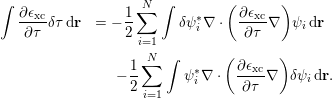 $$\begin{eqnarray}\displaystyle \int \displaystyle \frac{\unicode[STIX]{x2202}\unicode[STIX]{x1D716}_{\text{xc}}}{\unicode[STIX]{x2202}\unicode[STIX]{x1D70F}}\unicode[STIX]{x1D6FF}\unicode[STIX]{x1D70F}\,\text{d}\mathbf{r} & =-\displaystyle \frac{1}{2}\mathop{\sum }_{i=1}^{N}\int \unicode[STIX]{x1D6FF}\unicode[STIX]{x1D713}_{i}^{\ast }\unicode[STIX]{x1D6FB}\cdot \biggl(\displaystyle \frac{\unicode[STIX]{x2202}\unicode[STIX]{x1D716}_{\text{xc}}}{\unicode[STIX]{x2202}\unicode[STIX]{x1D70F}}\unicode[STIX]{x1D6FB}\biggr)\unicode[STIX]{x1D713}_{i}\,\text{d}\mathbf{r} & \displaystyle \nonumber\\ \displaystyle & \qquad -\displaystyle \frac{1}{2}\mathop{\sum }_{i=1}^{N}\int \unicode[STIX]{x1D713}_{i}^{\ast }\unicode[STIX]{x1D6FB}\cdot \biggl(\displaystyle \frac{\unicode[STIX]{x2202}\unicode[STIX]{x1D716}_{\text{xc}}}{\unicode[STIX]{x2202}\unicode[STIX]{x1D70F}}\unicode[STIX]{x1D6FB}\biggr)\unicode[STIX]{x1D6FF}\unicode[STIX]{x1D713}_{i}\,\text{d}\mathbf{r}. & \displaystyle\end{eqnarray}$$
Recall that the Kohn–Sham equation is obtained by variation with respect to
 $\unicode[STIX]{x1D6FF}\unicode[STIX]{x1D713}_{i}^{\ast }$
, thus the exchange-correlation ‘potential’
 $V_{\text{xc}}[\unicode[STIX]{x1D70C}]$
applied to the occupied orbital
 $\unicode[STIX]{x1D713}_{i}$
can be viewed as
 $$\begin{eqnarray}V_{\text{xc}}[\unicode[STIX]{x1D70C}]\unicode[STIX]{x1D713}_{i}=\biggl[\displaystyle \frac{\unicode[STIX]{x2202}\unicode[STIX]{x1D716}_{\text{xc}}}{\unicode[STIX]{x2202}\unicode[STIX]{x1D70C}}-2\unicode[STIX]{x1D6FB}\cdot \biggl(\displaystyle \frac{\unicode[STIX]{x2202}\unicode[STIX]{x1D716}_{\text{xc}}}{\unicode[STIX]{x2202}\unicode[STIX]{x1D70E}}\unicode[STIX]{x1D6FB}\unicode[STIX]{x1D70C}\biggr)-\displaystyle \frac{1}{2}\unicode[STIX]{x1D6FB}\cdot \biggl(\displaystyle \frac{\unicode[STIX]{x2202}\unicode[STIX]{x1D716}_{\text{xc}}}{\unicode[STIX]{x2202}\unicode[STIX]{x1D70F}}\unicode[STIX]{x1D6FB}\biggr)\biggr]\unicode[STIX]{x1D713}_{i}.\end{eqnarray}$$
Therefore, the exchange-correlation functional
 $V_{\text{xc}}[\unicode[STIX]{x1D70C}]$
is still independent of the orbitals, and can be defined only from the electron density as
 $$\begin{eqnarray}V_{\text{xc}}[\unicode[STIX]{x1D70C}]=\displaystyle \frac{\unicode[STIX]{x2202}\unicode[STIX]{x1D716}_{\text{xc}}}{\unicode[STIX]{x2202}\unicode[STIX]{x1D70C}}-2\unicode[STIX]{x1D6FB}\cdot \biggl(\displaystyle \frac{\unicode[STIX]{x2202}\unicode[STIX]{x1D716}_{\text{xc}}}{\unicode[STIX]{x2202}\unicode[STIX]{x1D70E}}\unicode[STIX]{x1D6FB}\unicode[STIX]{x1D70C}\biggr)-\displaystyle \frac{1}{2}\unicode[STIX]{x1D6FB}\cdot \biggl(\displaystyle \frac{\unicode[STIX]{x2202}\unicode[STIX]{x1D716}_{\text{xc}}}{\unicode[STIX]{x2202}\unicode[STIX]{x1D70F}}\unicode[STIX]{x1D6FB}\biggr).\end{eqnarray}$$
Strictly speaking this is no longer a potential, as it involves a differential operator
 $\unicode[STIX]{x1D6FB}\cdot ((\unicode[STIX]{x2202}\unicode[STIX]{x1D716}_{\text{xc}}/\unicode[STIX]{x2202}\unicode[STIX]{x1D70F})\unicode[STIX]{x1D6FB})$
acting on the orbitals. On the other hand, this is still a local operator, and can be treated in a similar way to our previous discussions.
For simplicity, for the rest of the paper we will neglect the spin degrees of freedom and consider the ‘spinless’ electrons. Hence all single-particle orbitals can be written as
 $\unicode[STIX]{x1D713}_{i}(\mathbf{r})$
instead of
 $\unicode[STIX]{x1D713}_{i}(\mathbf{x})$
. The numerical algorithms can be easily adapted to take into account the spin degrees of freedom.
2.4 Density matrix formulation
Consider a (one-body) Hamiltonian operator
 $H=-{\textstyle \frac{1}{2}}\unicode[STIX]{x1D6E5}+V$
. Assume that
 $H$
has a discrete spectrum and denote the eigenpairs of
 $H$
as
 $\{(\unicode[STIX]{x1D700}_{i},\unicode[STIX]{x1D713}_{i})\}$
:
 $$\begin{eqnarray}H\unicode[STIX]{x1D713}_{i}=\unicode[STIX]{x1D700}_{i}\unicode[STIX]{x1D713}_{i}.\end{eqnarray}$$
Assume that the system has
 $N$
electrons that occupy the first
 $N$
eigenstates according to Pauli’s exclusion principle. Here, for definiteness, we assume that
 $\unicode[STIX]{x1D700}_{N}<\unicode[STIX]{x1D700}_{N+1}$
to avoid degeneracy.
The Kohn–Sham energy functionals are invariant with respect to unitary rotations of the orbitals. The unitary rotation matrix is often referred to as the gauge degrees of freedom. Hence, the physical quantity is the subspace spanned by the occupied orbitals, instead of the individual eigenfunctions. This subspace
 $\operatorname{span}{\{\unicode[STIX]{x1D713}_{i}\}}_{i=1,\ldots ,N}$
is known as the Kohn–Sham occupied subspace and can be represented by the density matrix
 $$\begin{eqnarray}P=\mathop{\sum }_{i=1}^{N}|\unicode[STIX]{x1D713}_{i}\rangle \langle \unicode[STIX]{x1D713}_{i}|.\end{eqnarray}$$
Since the
 $\{\unicode[STIX]{x1D713}_{i}\}$
are orthonormal, we have
 $$\begin{eqnarray}P^{2}=\mathop{\sum }_{i,j=1}^{N}|\unicode[STIX]{x1D713}_{i}\rangle \langle \unicode[STIX]{x1D713}_{i}|\unicode[STIX]{x1D713}_{j}\rangle \langle \unicode[STIX]{x1D713}_{j}|=\mathop{\sum }_{i=1}^{N}|\unicode[STIX]{x1D713}_{i}\rangle \langle \unicode[STIX]{x1D713}_{i}|=P.\end{eqnarray}$$
Hence
 $P$
is self-adjoint and idempotent, and is the projection operator onto the occupied space. The kernel of
 $P$
, viewed as an integral operator, is given by
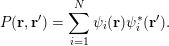 $$\begin{eqnarray}P(\mathbf{r},\mathbf{r}^{\prime })=\mathop{\sum }_{i=1}^{N}\unicode[STIX]{x1D713}_{i}(\mathbf{r})\unicode[STIX]{x1D713}_{i}^{\ast }(\mathbf{r}^{\prime }).\end{eqnarray}$$
In particular, we observe that the diagonal part of the kernel is just the electron density
 $$\begin{eqnarray}P(\mathbf{r},\mathbf{r})=\mathop{\sum }_{i=1}^{N}\unicode[STIX]{x1D713}_{i}(\mathbf{r})\unicode[STIX]{x1D713}_{i}^{\ast }(\mathbf{r})=\mathop{\sum }_{i=1}^{N}|\unicode[STIX]{x1D713}_{i}(\mathbf{r})|^{2}=\unicode[STIX]{x1D70C}(\mathbf{r}).\end{eqnarray}$$
Moreover the trace of
 $P$
is equal to the number of electrons:
 $$\begin{eqnarray}\operatorname{Tr}P=\int P(\mathbf{r},\mathbf{r})\,\text{d}\mathbf{r}=N.\end{eqnarray}$$
The Kohn–Sham equations can be reformulated in terms of the density matrix. Compared with the orbital representation, the density matrix is more intrinsic, as it is invariant with respect to the unitary rotation of the orbitals. In terms of numerical algorithms, use of the density matrix can also be advantageous, especially for large-scale problems, as we will discuss in Section 5.
Note that
 $P$
can be represented independent of the orbitals. Since
 $H$
is a self-adjoint operator, for any Borel-measurable function
 $f$
on the real line, a matrix function
 $f(H)$
can be defined using its spectral decomposition as
 $$\begin{eqnarray}f(H)=\mathop{\sum }_{i}f(\unicode[STIX]{x1D700}_{i})|\unicode[STIX]{x1D713}_{i}\rangle \langle \unicode[STIX]{x1D713}_{i}|.\end{eqnarray}$$
Recall that for simplicity we have assumed that the spectrum of
 $H$
is discrete. Thus, assuming that
 $\unicode[STIX]{x1D700}_{N}<\unicode[STIX]{x1D700}_{N+1}$
and the parameter
 $\unicode[STIX]{x1D707}\in \mathbb{R}$
satisfies
 $\unicode[STIX]{x1D700}_{N}\leq \unicode[STIX]{x1D707}<\unicode[STIX]{x1D700}_{N+1}$
, we have
 $$\begin{eqnarray}1_{(-\infty ,\unicode[STIX]{x1D707}]}(H)=\mathop{\sum }_{i}1_{(-\infty ,\unicode[STIX]{x1D707}]}(\unicode[STIX]{x1D700}_{i})|\unicode[STIX]{x1D713}_{i}\rangle \langle \unicode[STIX]{x1D713}_{i}|=\mathop{\sum }_{i:\unicode[STIX]{x1D700}_{i}\leq \unicode[STIX]{x1D707}}|\unicode[STIX]{x1D713}_{i}\rangle \langle \unicode[STIX]{x1D713}_{i}|=\mathop{\sum }_{i=1}^{N}|\unicode[STIX]{x1D713}_{i}\rangle \langle \unicode[STIX]{x1D713}_{i}|=P.\end{eqnarray}$$
We conclude with
 $$\begin{eqnarray}P=1_{(-\infty ,\unicode[STIX]{x1D707}]}(H),\end{eqnarray}$$
where the right-hand side is the spectral projection onto the interval
 $(\!-\infty ,\unicode[STIX]{x1D707}]$
. Here
 $\unicode[STIX]{x1D707}$
is known as the Fermi level or the chemical potential.
2.5 Non-local functionals
Let us now introduce the non-local exchange-correlation functionals, which are on the fourth and fifth rungs of Perdew’s ladder above the semi-local ones introduced in Section 2.2. These more complex density functionals can improve the fidelity of DFT, but they may significantly increase the computational cost at the same time.
On the fourth rung are the so-called hybrid density functionals, such as B3LYP (Becke Reference Becke1993), PBE0 (Perdew, Ernzerhof and Burke Reference Perdew, Ernzerhof and Burke1996b ) and HSE (Heyd et al. Reference Heyd, Scuseria and Ernzerhof2003). They have been shown to improve the accuracy of Kohn–Sham DFT calculations, such as the computation of adsorption energies for molecules on surfaces, and molecular frontier level alignment relative to metals and semiconductors. This is achieved by incorporating a fraction of the Hartree–Fock exact exchange or screened exchange operator into the Kohn–Sham Hamiltonian. The hybrid energy functionals depend not only on the density but also on the density matrix, and hence, strictly speaking, they are no longer ‘pure’ density functionals. A hybrid functional typically takes the following form of hybridization based on a density-based exchange energy and the exact exchange energy (Becke Reference Becke1993, Heyd et al. Reference Heyd, Scuseria and Ernzerhof2003):
 $$\begin{eqnarray}E_{\text{xc}}[P]=E_{\text{c}}[\unicode[STIX]{x1D70C}]+(1-\unicode[STIX]{x1D6FC})E_{\text{x}}[\unicode[STIX]{x1D70C}]+\unicode[STIX]{x1D6FC}E_{\text{x}}^{\text{EX}}[P].\end{eqnarray}$$
Here
 $\unicode[STIX]{x1D6FC}$
is a parameter for the fraction of the non-local exchange contribution, and
 $E_{\text{x}}$
and
 $E_{\text{c}}$
are the exchange and correlation parts (see e.g. Martin Reference Martin2008 for the separation of the exchange-correlation functional into the exchange and correlation components, respectively) from semi-local functionals, such as GGA functionals.
 $E_{\text{x}}^{\text{EX}}[P]$
is the (screened) Hartree–Fock exchange energy corresponding to the density matrix
 $P$
:
 $$\begin{eqnarray}E_{\text{x}}^{\text{EX}}[P]=-\displaystyle \frac{1}{2}\iint |P(\mathbf{r},\mathbf{r}^{\prime })|^{2}K(\mathbf{r},\mathbf{r}^{\prime })\,\text{d}\mathbf{r}\,\text{d}\mathbf{r}^{\prime },\end{eqnarray}$$
where
 $K(\mathbf{r},\mathbf{r}^{\prime })$
is the kernel for the electron–electron interaction. For example, for Hartree–Fock exchange,
 $K(\mathbf{r},\mathbf{r}^{\prime })=v_{C}(\mathbf{r},\mathbf{r}^{\prime })=1/|\mathbf{r}-\mathbf{r}^{\prime }|$
is the Coulomb kernel. In theories with screened Fock exchange interactions (Heyd et al.
Reference Heyd, Scuseria and Ernzerhof2003),
 $K$
can be a screened Coulomb kernel with
 $K(\mathbf{r},\mathbf{r}^{\prime })=\text{erfc}(\unicode[STIX]{x1D6FC}_{s}|\mathbf{r}-\mathbf{r}^{\prime }|)/|\mathbf{r}-\mathbf{r}^{\prime }|$
, where
 $\unicode[STIX]{x1D6FC}_{s}$
is the inverse screening length parameter.
On the fifth rung of the ladder, we have functionals that depend not only on the density and occupied Kohn–Sham orbitals but also on other quantities such as the eigenvalues and virtual orbitals of the Kohn–Sham effective Hamiltonian. They are sometimes referred to as orbital functionals. Examples of such functionals include the double hybrid functionals (Grimme Reference Grimme2006, Zhang, Xu and Goddard III Reference Zhang, Xu and Goddard2009, Goerigk and Grimme Reference Goerigk and Grimme2014), van der Waals functionals (Dion et al. Reference Dion, Rydberg, Schröder, Langreth and Lundqvist2004), random phase approximation (RPA) functionals (Ren, Rinke, Joas and Scheffler Reference Ren, Rinke, Joas and Scheffler2012b , Chen et al. Reference Chen, Voora, Agee, Balasubramani and Furche2017), and other functionals based on many-body perturbation theory (see e.g. Mori-Sánchez, Wu and Yang Reference Mori-Sánchez, Wu and Yang2005, Ren, Rinke, Scuseria and Scheffler Reference Ren, Rinke, Scuseria and Scheffler2013, Zhang, Rinke and Scheffler Reference Zhang, Rinke and Scheffler2016).
For an example of rung-
 $5$
functionals, let us consider the RPA functional, for which the exchange-correlation
 $E_{\text{xc}}=E_{\text{x}}+E_{\text{c}}$
consists of the exact exchange and the random phase approximation (Bohm and Pines Reference Bohm and Pines1953, Gell-Mann and Brueckner Reference Gell-Mann and Brueckner1957) of the correlation energy
 $E_{\text{c}}$
given by
 $$\begin{eqnarray}E_{\text{c}}^{\text{RPA}}=\displaystyle \frac{1}{2\unicode[STIX]{x1D70B}}\int _{0}^{\infty }\operatorname{Tr}[\ln (1-\hat{\unicode[STIX]{x1D712}}^{0}(\text{i}\unicode[STIX]{x1D714})v_{C})+\hat{\unicode[STIX]{x1D712}}^{0}(\text{i}\unicode[STIX]{x1D714})v_{C}]\,\text{d}\unicode[STIX]{x1D714},\end{eqnarray}$$
where
 $v_{C}$
is the Coulomb kernel in (2.25), and
 $\hat{\unicode[STIX]{x1D712}}^{0}$
is the dynamic polarizability operator
 $$\begin{eqnarray}\displaystyle \hat{\unicode[STIX]{x1D712}}^{0}(\mathbf{r},\mathbf{r}^{\prime },\text{i}\unicode[STIX]{x1D714})=\mathop{\sum }_{i}^{\text{occ}}\mathop{\sum }_{a}^{\text{vir}}\displaystyle \frac{\unicode[STIX]{x1D713}_{i}^{\ast }(\mathbf{r})\unicode[STIX]{x1D713}_{a}(\mathbf{r})\unicode[STIX]{x1D713}_{a}^{\ast }(\mathbf{r}^{\prime })\unicode[STIX]{x1D713}_{i}(\mathbf{r}^{\prime })}{\unicode[STIX]{x1D700}_{i}-\unicode[STIX]{x1D700}_{a}-\text{i}\unicode[STIX]{x1D714}}+\text{c.c.} & & \displaystyle\end{eqnarray}$$
Here ‘occ’ and ‘vir’ denote the set of occupied and virtual orbitals, respectively, and c.c. stands for the complex conjugate of the previous term. Approximation of the correlation is obtained by applying random phase approximation combined with the adiabatic connection (Langreth and Perdew Reference Langreth and Perdew1975, Gunnarsson and Lundqvist Reference Gunnarsson and Lundqvist1976, Ren et al. Reference Ren, Rinke, Joas and Scheffler2012b ). Note that equation (2.50) contains the virtual orbitals and also the Kohn–Sham orbital energies, which result from the dynamic linear response of the system.
The Kohn–Sham equations of non-local functionals involve non-local operators (hence the name non-local functionals). For rung-
 $4$
functionals, the Kohn–Sham equations take the form
 $$\begin{eqnarray}\displaystyle & \displaystyle H[P]\unicode[STIX]{x1D713}_{i}=\biggl(-\displaystyle \frac{1}{2}\unicode[STIX]{x1D6E5}+V_{\text{ext}}+V_{\text{Hxc}}[\unicode[STIX]{x1D70C}]+\unicode[STIX]{x1D6FC}V_{\text{x}}^{\text{EX}}[P]\biggr)\unicode[STIX]{x1D713}_{i}=\unicode[STIX]{x1D700}_{i}\unicode[STIX]{x1D713}_{i}, & \displaystyle \nonumber\\ \displaystyle & \displaystyle \int \unicode[STIX]{x1D713}_{i}^{\ast }(\mathbf{r})\unicode[STIX]{x1D713}_{j}(\mathbf{r})\,\text{d}\mathbf{r}=\unicode[STIX]{x1D6FF}_{ij},\quad P(\mathbf{r},\mathbf{r}^{\prime })=\mathop{\sum }_{i=1}^{N}\unicode[STIX]{x1D713}_{i}(\mathbf{r})\unicode[STIX]{x1D713}_{i}^{\ast }(\mathbf{r}^{\prime }). & \displaystyle\end{eqnarray}$$
Here
 $V_{\text{Hxc}}$
is the Hartree and exchange-correlation contribution from the electron density
 $\unicode[STIX]{x1D70C}$
only, and
 $V_{\text{x}}^{\text{EX}}[P]$
is derived from the exact exchange functional
 $E_{\text{x}}^{\text{EX}}[P]$
, with kernel
 $$\begin{eqnarray}V_{\text{x}}^{\text{EX}}[P](\mathbf{r},\mathbf{r}^{\prime })=-P(\mathbf{r},\mathbf{r}^{\prime })K(\mathbf{r},\mathbf{r}^{\prime }).\end{eqnarray}$$
 $V_{\text{x}}^{\text{EX}}[P]$
is often called the Fock exchange operator, and is negative semi-definite. Equation (2.51) is called the Hartree–Fock-like equation. In this case the Kohn–Sham map in equation (2.34) becomes the generalized Kohn–Sham map from
 $V_{\text{eff}}$
to the density matrix
 $P$
. The numerical treatment of the exact exchange term, as well as the Hartree–Fock-like equation, will be discussed in detail in Section 6.
The self-consistency for RPA functionals is much more complicated, since the functional involves virtual orbitals and orbital energies. Most current strategies are to first obtain the effective Hamiltonian and corresponding Kohn–Sham orbitals based on a semi-local or hybrid functional, and then calculate the RPA correlation in a post-processing step. Self-consistency calculations have been performed using the optimized effective potential (OEP) framework (Godby, Schlüter and Sham Reference Godby, Schlüter and Sham1986, Reference Godby, Schlüter and Sham1988, Fukazawa and Akai Reference Fukazawa and Akai2015) or more recently the generalized optimized effective potential approach (Jin et al.
Reference Jin, Zhang, Chen, Su and Yang2017), but they come with considerable numerical effort. Finding an efficient approach for self-consistent treatment of RPA functionals is an active research area, and in this review we will not discuss self-consistency for rung-
 $5$
functionals in detail.
2.6 Finite temperature density functional theory
The Kohn–Sham density functional theory for ground-state quantum systems discussed so far can be extended to systems at finite temperature (Mermin Reference Mermin1965). Instead of a variational principle for the ground-state energy, the functional for free energy is minimized with respect to the density matrix, that is,
 $$\begin{eqnarray}\displaystyle {\mathcal{F}}_{\unicode[STIX]{x1D6FD}}[\unicode[STIX]{x1D70C}] & = & \displaystyle \inf _{\substack{ P\in {\mathcal{D}} \\ P\mapsto \unicode[STIX]{x1D70C}}}\bigg(\displaystyle \frac{1}{2}\operatorname{Tr}((-\unicode[STIX]{x1D6E5})P)+\unicode[STIX]{x1D6FD}^{-1}\operatorname{Tr}(P\ln P+(I-P)\ln (I-P))\nonumber\\ \displaystyle & & \displaystyle \qquad \qquad +\displaystyle \frac{1}{2}\int \displaystyle \frac{\unicode[STIX]{x1D70C}(\mathbf{r})\unicode[STIX]{x1D70C}(\mathbf{r}^{\prime })}{|\mathbf{r}-\mathbf{r}^{\prime }|}\,\text{d}\mathbf{r}\,\text{d}\mathbf{r}^{\prime }+E_{\text{xc},\unicode[STIX]{x1D6FD}}[\unicode[STIX]{x1D70C}]\bigg),\end{eqnarray}$$
where
 $\operatorname{Tr}(P\ln P+(I-P)\ln (I-P))$
is the Fermi–Dirac entropy (Parr and Yang Reference Parr and Yang1989) and
 ${\mathcal{D}}$
is the set of all one-particle density matrices for an
 $N$
-electron system:
 $$\begin{eqnarray}{\mathcal{D}}=\{P\in {\mathcal{B}}(L^{2}(\mathbb{R}^{3}))\;:\;P=P^{\ast },0\preccurlyeq P\preccurlyeq I,\operatorname{Tr}P=N\}.\end{eqnarray}$$
Here
 ${\mathcal{B}}(L^{2}(\mathbb{R}^{3}))$
stands for the bounded operators on
 $L^{2}(\mathbb{R}^{3})$
and the constraint
 $0\preccurlyeq P\preccurlyeq I$
comes from the Pauli exclusion principle. To see this, let the eigen-decomposition of
 $P$
be
 $$\begin{eqnarray}P=\mathop{\sum }_{i}f_{i}|\unicode[STIX]{x1D713}_{i}\rangle \langle \unicode[STIX]{x1D713}_{i}|.\end{eqnarray}$$
The constraints
 $0\preccurlyeq P\preccurlyeq I$
and
 $\operatorname{Tr}P=N$
imply that the occupation number
 $\{f_{i}\}$
satisfies
 $$\begin{eqnarray}0\leq f_{i}\leq 1\quad \text{and}\quad \mathop{\sum }_{i}f_{i}=N.\end{eqnarray}$$
Thus no state is occupied by more than one electron. Here the summation is performed over all single-particle orbitals, rather than only the occupied ones.
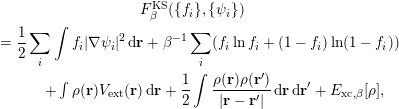
We can write the variational problem more explicitly in terms of the
 $(f_{i},\unicode[STIX]{x1D713}_{i})$
as
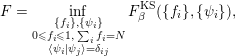 $$\begin{eqnarray}F=\inf _{\substack{ \{f_{i}\},\{\unicode[STIX]{x1D713}_{i}\} \\ 0\leq f_{i}\leq 1,\;\mathop{\sum }_{i}f_{i}=N \\ \langle \unicode[STIX]{x1D713}_{i}|\unicode[STIX]{x1D713}_{j}\rangle =\unicode[STIX]{x1D6FF}_{ij}}}F_{\unicode[STIX]{x1D6FD}}^{\text{KS}}(\{f_{i}\},\{\unicode[STIX]{x1D713}_{i}\}),\end{eqnarray}$$
with
 $$\begin{eqnarray}\displaystyle & F_{\unicode[STIX]{x1D6FD}}^{\text{KS}}(\{f_{i}\},\{\unicode[STIX]{x1D713}_{i}\}) & \displaystyle \nonumber\\ \displaystyle & \quad =\displaystyle \frac{1}{2}\mathop{\sum }_{i}\int f_{i}|\unicode[STIX]{x1D6FB}\unicode[STIX]{x1D713}_{i}|^{2}\,\text{d}\mathbf{r}+\unicode[STIX]{x1D6FD}^{-1}\mathop{\sum }_{i}(f_{i}\ln f_{i}+(1-f_{i})\ln (1-f_{i})) & \displaystyle \nonumber\\ \displaystyle & \quad \qquad +\int \unicode[STIX]{x1D70C}(\mathbf{r})V_{\text{ext}}(\mathbf{r})\,\text{d}\mathbf{r}+\displaystyle \frac{1}{2}\int \displaystyle \frac{\unicode[STIX]{x1D70C}(\mathbf{r})\unicode[STIX]{x1D70C}(\mathbf{r}^{\prime })}{|\mathbf{r}-\mathbf{r}^{\prime }|}\,\text{d}\mathbf{r}\,\text{d}\mathbf{r}^{\prime }+E_{\text{xc},\unicode[STIX]{x1D6FD}}[\unicode[STIX]{x1D70C}], & \displaystyle\end{eqnarray}$$
and the density is given by
 $$\begin{eqnarray}\unicode[STIX]{x1D70C}(\mathbf{r})=\mathop{\sum }_{i}f_{i}|\unicode[STIX]{x1D713}_{i}(\mathbf{r})|^{2}.\end{eqnarray}$$
In principle, the exchange-correlation functional for the finite temperature
 $E_{\text{xc},\unicode[STIX]{x1D6FD}}[\unicode[STIX]{x1D70C}]$
depends on
 $\unicode[STIX]{x1D6FD}$
and also has a ladder of approximation schemes like the zero temperature case. However, most finite temperature DFT calculations in practice still use the temperature-independent exchange-correlation functional at the semi-local level. The zero and finite temperature functional approximations share the same mathematical structure. Hence, for the purpose of our discussions, we will not explicitly distinguish them below.
We now consider the Kohn–Sham equations for the finite temperature functional (2.53). As the functional involves minimization with respect to the density matrix
 $P$
, it is more convenient to consider the combined minimization of density and the associated density matrix:
 $$\begin{eqnarray}\displaystyle & & \displaystyle \inf _{P\in {\mathcal{D}}}\bigg(\displaystyle \frac{1}{2}\operatorname{Tr}((-\unicode[STIX]{x1D6E5})P)+\unicode[STIX]{x1D6FD}^{-1}\operatorname{Tr}(P\ln P+(I-P)\ln (I-P))\nonumber\\ \displaystyle & & \displaystyle \qquad \qquad +\displaystyle \frac{1}{2}\int \displaystyle \frac{\unicode[STIX]{x1D70C}(\mathbf{r})\unicode[STIX]{x1D70C}(\mathbf{r}^{\prime })}{|\mathbf{r}-\mathbf{r}^{\prime }|}\,\text{d}\mathbf{r}\,\text{d}\mathbf{r}^{\prime }+E_{\text{xc},\unicode[STIX]{x1D6FD}}[\unicode[STIX]{x1D70C}]\bigg),\end{eqnarray}$$
where
 $\unicode[STIX]{x1D70C}$
is given by the diagonal of the density matrix
 $P$
. Taking the variation with respect to
 $P$
, we obtain the Euler–Lagrange equation
 $$\begin{eqnarray}H_{\unicode[STIX]{x1D6FD}}^{\text{KS}}[\unicode[STIX]{x1D70C}]+\unicode[STIX]{x1D6FD}^{-1}(\ln P-\ln (I-P))-\unicode[STIX]{x1D707}=0,\end{eqnarray}$$
where
 $\unicode[STIX]{x1D707}$
is the Lagrange multiplier associated with the constraint
 $\operatorname{Tr}P=N$
and the effective Hamiltonian is given as in the zero temperature case (cf. (2.24)), that is,
 $$\begin{eqnarray}H_{\unicode[STIX]{x1D6FD}}^{\text{KS}}[\unicode[STIX]{x1D70C}]=-\displaystyle \frac{1}{2}\unicode[STIX]{x1D6E5}+V_{\text{ext}}+V_{H}[\unicode[STIX]{x1D70C}]+V_{\text{xc},\unicode[STIX]{x1D6FD}}[\unicode[STIX]{x1D70C}].\end{eqnarray}$$
Solving (2.61) for
 $P$
, we get
 $$\begin{eqnarray}P=[I+\exp (\unicode[STIX]{x1D6FD}(H_{\unicode[STIX]{x1D6FD}}^{\text{KS}}[\unicode[STIX]{x1D70C}]-\unicode[STIX]{x1D707}))]^{-1}.\end{eqnarray}$$
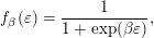
Letting
 $f_{\unicode[STIX]{x1D6FD}}$
be the Fermi–Dirac distribution function
 $$\begin{eqnarray}f_{\unicode[STIX]{x1D6FD}}(\unicode[STIX]{x1D700})=\displaystyle \frac{1}{1+\exp (\unicode[STIX]{x1D6FD}\unicode[STIX]{x1D700})},\end{eqnarray}$$
we arrive at the self-consistent equation
 $$\begin{eqnarray}P=f_{\unicode[STIX]{x1D6FD}}(H_{\unicode[STIX]{x1D6FD}}^{\text{KS}}[\unicode[STIX]{x1D70C}]-\unicode[STIX]{x1D707})=\mathop{\sum }_{i}f_{\unicode[STIX]{x1D6FD}}(\unicode[STIX]{x1D700}_{i}-\unicode[STIX]{x1D707})|\unicode[STIX]{x1D713}_{i}\rangle \langle \unicode[STIX]{x1D713}_{i}|,\end{eqnarray}$$
where
 $\unicode[STIX]{x1D700}_{i}$
and
 $\unicode[STIX]{x1D713}_{i}$
are the eigenvalue and associated eigenfunction of
 $H_{\unicode[STIX]{x1D6FD}}^{\text{KS}}[\unicode[STIX]{x1D70C}]$
respectively. We see that the occupation number is given by
 $$\begin{eqnarray}f_{i}=f_{\unicode[STIX]{x1D6FD}}(\unicode[STIX]{x1D700}_{i}-\unicode[STIX]{x1D707})=\displaystyle \frac{1}{1+\exp (\unicode[STIX]{x1D6FD}(\unicode[STIX]{x1D700}_{i}-\unicode[STIX]{x1D707}))}.\end{eqnarray}$$
Thus
 $f_{i}\in (0,1)$
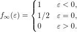
, and all eigenstates are occupied with a fractional number. Also, notice that as
 $\unicode[STIX]{x1D6FD}\rightarrow \infty$
(zero temperature limit),
 $f_{\unicode[STIX]{x1D6FD}}$
converges to the function
 $f_{\infty }$
:
 $$\begin{eqnarray}f_{\infty }(\unicode[STIX]{x1D700})=\left\{\begin{array}{@{}ll@{}}1\quad & \unicode[STIX]{x1D700}<0,\\ 1/2\quad & \unicode[STIX]{x1D700}=0,\\ 0\quad & \unicode[STIX]{x1D700}>0.\end{array}\right.\end{eqnarray}$$
Let
 $\unicode[STIX]{x1D707}_{\unicode[STIX]{x1D6FD}}$
denote the Lagrange multiplier for the inverse temperature
 $\unicode[STIX]{x1D6FD}$
, where we make the dependence on
 $\unicode[STIX]{x1D6FD}$
explicit. In the limit, we can show that (as before, we assume
 $\unicode[STIX]{x1D700}_{N}<\unicode[STIX]{x1D700}_{N+1}$
)
 $$\begin{eqnarray}\lim _{\unicode[STIX]{x1D6FD}\rightarrow \infty }\unicode[STIX]{x1D707}_{\unicode[STIX]{x1D6FD}}=\displaystyle \frac{1}{2}(\unicode[STIX]{x1D700}_{N}+\unicode[STIX]{x1D700}_{N+1})=:\unicode[STIX]{x1D707}_{\infty }.\end{eqnarray}$$
Therefore, the density matrix of finite temperature is consistent with the definition of the chemical potential at zero temperature. Compared to equation (2.46), we may also write
 $$\begin{eqnarray}P=f_{\infty }(H-\unicode[STIX]{x1D707}_{\infty }).\end{eqnarray}$$
2.7 Pseudopotential approximation
In typical electronic structure calculations, not all electrons play the same role. In a single-particle picture, it is well known that the core electrons (i.e. orbitals with relatively low energies) are barely affected by the chemical environment. It is therefore desirable to remove the core electrons from the actual computation, and solve the Kohn–Sham equations for valence electrons (i.e. orbitals with relatively high energies) only. Another difficulty in all-electron calculations lies in the treatment of the singular Coulomb interaction between nuclei and electrons, which introduces a cusp in the Kohn–Sham orbitals at each atomic position. The electron–nucleus cusp makes uniform basis functions such as planewaves (to be discussed in Section 3.1) very inefficient for all-electron calculations.
Hence the pseudopotential approximation is introduced to solve both issues simultaneously, which is widely used especially in solid-state physics and materials science. Although this is not a systematically controlled approximation, numerical results indicate that the error introduced by the use of the pseudopotential can be much smaller compared to other sources of error in Kohn–Sham DFT calculations. Simply speaking, the use of pseudopotentials has the following benefits.
(1) The number of Kohn–Sham orbitals depends only on the number of valence electrons. This is particularly important for heavy elements, where each atom involves several tens of electrons, while the number of valence electrons can be much smaller.
(2) The valence electron orbitals are typically smoother than the core electron orbitals, and hence require a smaller number of basis functions such as planewaves to resolve.
(3) After removing the core electrons, the resulting pseudo-valence electron orbitals have fewer nodes near the nuclei. This further enhances the smoothness of the orbitals and reduces computational cost.
Below we introduce the basic idea of the norm-conserving pseudopotential (Hamann, Schlüter and Chiang Reference Hamann, Schlüter and Chiang1979, Troullier and Martins Reference Troullier and Martins1991) – the earliest and still the most widely used form of pseudopotential. With some abuse of notation, in this section we use Cartesian coordinates
 $(r_{1},r_{2},r_{3})^{\top }$
and spherical coordinates
 $(r,\unicode[STIX]{x1D703},\unicode[STIX]{x1D719})^{\top }$
for the same electron position
 $\mathbf{r}$
interchangeably. When a function
 $f(\mathbf{r})$
depends only on the radial distance
 $r$
, we will not distinguish between
 $f(\mathbf{r})$
and
 $f(r)$
. Similarly, if
 $f(\mathbf{r})$
depends only on the angular variables
 $\unicode[STIX]{x1D703}$
and
 $\unicode[STIX]{x1D719}$
, we will not distinguish between
 $f(\mathbf{r})$
and
 $f(\unicode[STIX]{x1D703},\unicode[STIX]{x1D719})$
.
For a single atom at the origin
 $\mathbf{R}=\mathbf{0}$
, the electron–nucleus interaction becomes
 $V_{\text{ext}}(r)=-Z/r$
, where
 $Z$
is the charge of the nucleus. Consider the atomic Kohn–Sham equation
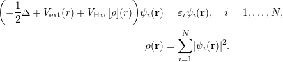 $$\begin{eqnarray}\displaystyle \biggl(-\displaystyle \frac{1}{2}\unicode[STIX]{x1D6E5}+V_{\text{ext}}(r)+V_{\text{Hxc}}[\unicode[STIX]{x1D70C}](r)\biggr)\unicode[STIX]{x1D713}_{i}(\mathbf{r}) & = & \displaystyle \unicode[STIX]{x1D700}_{i}\unicode[STIX]{x1D713}_{i}(\mathbf{r}),\quad i=1,\ldots ,N,\nonumber\\ \displaystyle \unicode[STIX]{x1D70C}(\mathbf{r}) & = & \displaystyle \mathop{\sum }_{i=1}^{N}|\unicode[STIX]{x1D713}_{i}(\mathbf{r})|^{2}.\end{eqnarray}$$
Here
 $V_{\text{Hxc}}$
includes the contribution from the Hartree and exchange-correlation interactions, which also depend only on the radial distance
 $r$
if the electron density
 $\unicode[STIX]{x1D70C}(\mathbf{r})=\unicode[STIX]{x1D70C}(r)$
satisfies spherical symmetry. However, some single-particle orbital
 $\unicode[STIX]{x1D713}_{i}(\mathbf{r})$
might not be spherically symmetric and thus still depend on all components of
 $\mathbf{r}$
.
Let us separate the
 $N$
Kohn–Sham orbitals into two groups: core electron orbitals
 $\{\unicode[STIX]{x1D713}_{i}\}_{i=1}^{N_{c}}$
and valence electron orbitals
 $\{\unicode[STIX]{x1D713}_{i}\}_{i=N_{c}+1}^{N}$
. This also defines the number of valence orbitals
 $N_{v}:=N-N_{c}$
. The goal of the pseudopotential approximation is to find an operator
 $V_{\text{ps}}$
which is defined to satisfy the following modified equation:
 $$\begin{eqnarray}\displaystyle \biggl(-\displaystyle \frac{1}{2}\unicode[STIX]{x1D6E5}+V_{\text{ps}}+V_{\text{Hxc}}[\widetilde{\unicode[STIX]{x1D70C}}](r)\biggr)\widetilde{\unicode[STIX]{x1D713}}_{i}(\mathbf{r}) & = & \displaystyle \widetilde{\unicode[STIX]{x1D700}}_{i}\widetilde{\unicode[STIX]{x1D713}}_{i}(\mathbf{r}),\quad i=1,\ldots ,N_{v},\nonumber\\ \displaystyle \widetilde{\unicode[STIX]{x1D70C}}(\mathbf{r}) & = & \displaystyle \mathop{\sum }_{i=1}^{N_{v}}|\widetilde{\unicode[STIX]{x1D713}}_{i}(\mathbf{r})|^{2}.\end{eqnarray}$$
The orbitals
 $\{\widetilde{\unicode[STIX]{x1D713}}_{i}\}$
are called pseudo-valence orbitals, and the eigenvalues
 $\{\widetilde{\unicode[STIX]{x1D700}}_{i}\}$
are called pseudo-valence eigenvalues, respectively. Note that we need only solve
 $N_{v}$
instead of
 $N$
orbitals. Furthermore, we require that the solution to equation (2.70) satisfies the following conditions, which are called the Hamann–Schlüter–Chiang (HSC) conditions (Hamann et al.
Reference Hamann, Schlüter and Chiang1979).
(1) The pseudo-valence eigenvalues agree with the real valence eigenvalues:
(2.71) $$\begin{eqnarray}\widetilde{\unicode[STIX]{x1D700}}_{i}=\unicode[STIX]{x1D700}_{i+N_{c}},\quad i=1,\ldots ,N_{v}.\end{eqnarray}$$
(2) The pseudo-valence orbitals agree with the real valence orbitals outside a given radius
$r_{c}$
: (2.72)$$\begin{eqnarray}\widetilde{\unicode[STIX]{x1D713}}_{i}(\mathbf{r})=\unicode[STIX]{x1D713}_{i+N_{c}}(\mathbf{r}),\quad r\geq r_{c},\quad i=1,\ldots ,N_{v}.\end{eqnarray}$$
(3) The pseudo-valence orbitals are normalized, that is,
(2.73)$$\begin{eqnarray}\langle \widetilde{\unicode[STIX]{x1D713}_{i}}|\widetilde{\unicode[STIX]{x1D713}_{i}}\rangle =1.\end{eqnarray}$$




In particular, condition (3) is called the norm-conservation condition, which leads to the name of this class of pseudopotential approximation. Although the pseudo-valence orbitals should form an orthonormal set of functions, in the discussion below we will associate the orbitals with spherical harmonic functions that are orthogonal to each other. Hence the orthogonality condition will be automatically satisfied, and only the normalization condition is imposed here.
The choice of pseudopotential satisfying the HSC conditions is by no means unique. In order to construct a
 $V_{\text{ps}}$
satisfying the HSC conditions, for simplicity let us first consider the case where
 $N_{v}=1$
. Note that the pseudo-valence orbital
 $\widetilde{\unicode[STIX]{x1D713}}_{1}$
now becomes the ground state of equation (2.70), and must therefore be a nodeless function (Lieb and Loss Reference Lieb and Loss2001). On the other hand, the real valence orbital
 $\unicode[STIX]{x1D713}_{1}$
should be orthogonal to all core orbitals, and therefore must have nodes within the core region
 $r\leq r_{c}$
. Hence the real and pseudo-valence orbitals have qualitatively different shapes within the core region, but this does not affect the shape of the valence orbitals outside the core region due to HSC condition (2). When
 $N_{v}=1$
, the valence orbital is expected to be spherically symmetric (called an
 $s$
-orbital):
 $$\begin{eqnarray}\unicode[STIX]{x1D713}_{N_{c}+1}(\mathbf{r})=\unicode[STIX]{x1D711}(r),\end{eqnarray}$$
where we use the notation
 $\unicode[STIX]{x1D711}(r)$
to emphasize that the valence orbital depends only on the radial distance
 $r$
and is real. Similarly the pseudo-valence orbital should also be spherically symmetric and we denote
 $$\begin{eqnarray}\widetilde{\unicode[STIX]{x1D713}}_{1}(\mathbf{r})=\widetilde{\unicode[STIX]{x1D711}}(r).\end{eqnarray}$$
In such a case,
 $V_{\text{ps}}$
can be chosen to be a local potential that depends only on
 $r$
, denoted by
 $V_{\text{loc}}(r)$
. To see this, we may simply choose a pseudo-valence orbital
 $\widetilde{\unicode[STIX]{x1D711}}(r)$
such that HSC conditions (2) and (3) are satisfied. In order to satisfy HSC condition (1), we may invert the Schrödinger equation (2.70) as
 $$\begin{eqnarray}V_{\text{loc}}(r)=\unicode[STIX]{x1D700}_{1}+\displaystyle \frac{\unicode[STIX]{x1D6E5}_{\mathbf{r}}\widetilde{\unicode[STIX]{x1D713}}_{1}(\mathbf{r})}{2\unicode[STIX]{x1D713}_{1}(\mathbf{r})}-V_{\text{Hxc}}[\widetilde{\unicode[STIX]{x1D70C}}](r)=\unicode[STIX]{x1D700}_{1}+\displaystyle \frac{1}{2r^{2}}\displaystyle \frac{\unicode[STIX]{x2202}}{\unicode[STIX]{x2202}r}\biggl(r^{2}\displaystyle \frac{\unicode[STIX]{x2202}\widetilde{\unicode[STIX]{x1D711}}}{\unicode[STIX]{x2202}r}\biggr)-V_{\text{Hxc}}[\widetilde{\unicode[STIX]{x1D70C}}](r).\end{eqnarray}$$
Note that
 $V_{\text{loc}}(r)$
depends only on the radial distance due to the assumptions of
 $\widetilde{\unicode[STIX]{x1D713}}_{1}$
and
 $\widetilde{\unicode[STIX]{x1D70C}}$
. Figure 2.4 shows an example comparing the valence 2s orbital of the fluorine atom (F) in an all-electron calculation, and the pseudo-valence orbital using a Troullier–Martins pseudopotential (Troullier and Martins Reference Troullier and Martins1991). We find that the orbital becomes significantly smoother in the pseudopotential approximation. In particular, the pseudo-valence orbital is nodeless in the core region.
Comparison of the 2s orbital of the fluorine atom in an all-electron and a pseudopotential calculation. The cut-off radius
 $r_{c}$
is set to
 $1.0$
a.u.
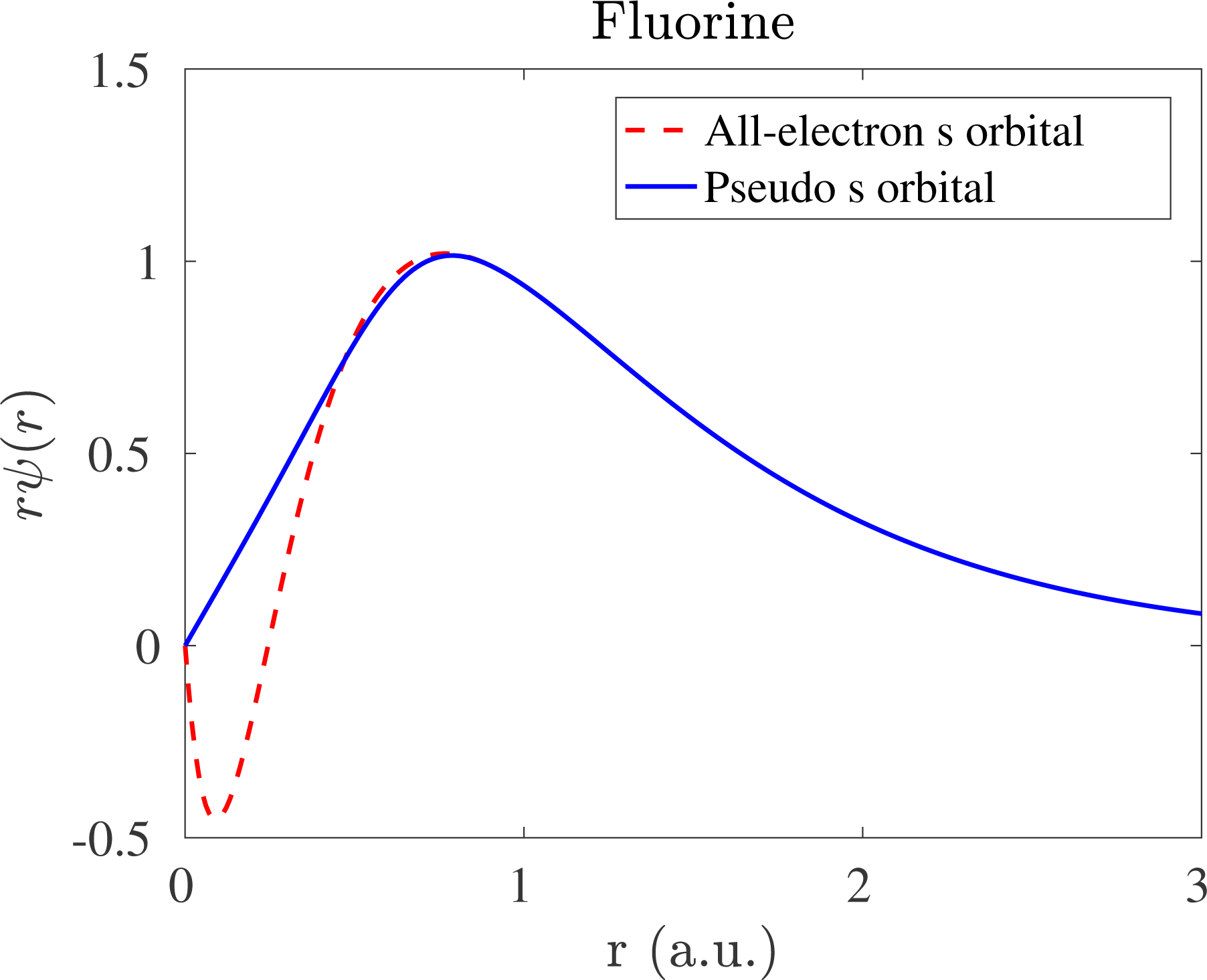
However, such a strategy becomes problematic when
 $N_{v}>1$
. To see this, following the notation of solutions to hydrogen-like atoms (Landau and Lifshitz Reference Landau and Lifshitz1991), we first relabel the real and pseudo-valence orbitals as (here
 $\hat{\mathbf{r}}=\mathbf{r}/r$
)
 $$\begin{eqnarray}\unicode[STIX]{x1D713}_{lm}(\mathbf{r})=\unicode[STIX]{x1D711}_{l}(r)Y_{lm}(\hat{\mathbf{r}}),\quad \widetilde{\unicode[STIX]{x1D713}}_{lm}(\mathbf{r})=\widetilde{\unicode[STIX]{x1D711}}_{l}(r)Y_{lm}(\hat{\mathbf{r}}).\end{eqnarray}$$
The integers
 $l,m$
are called the azimuthal and magnetic quantum numbers, respectively. For each azimuthal quantum number
 $l$
, the admissible integer
 $m$
should satisfy
 $-l\leq m\leq l$
. Compared to the complete solution for hydrogen-like atoms, the choice of ‘valence electron’ fixes the principal quantum number implicitly. The radial parts
 $\unicode[STIX]{x1D711}_{l},\widetilde{\unicode[STIX]{x1D711}}_{l}$
are real.
 $Y_{lm}(\hat{\mathbf{r}})$
is a spherical harmonic function defined on
 $\mathbb{S}^{2}$
, which can also be viewed as a function
 $Y_{lm}(\unicode[STIX]{x1D703},\unicode[STIX]{x1D711})$
that depends only on the angular degrees of freedom in spherical coordinates. The spherical harmonic functions satisfy the orthonormality condition
 $$\begin{eqnarray}\displaystyle & & \displaystyle \int _{\mathbb{S}^{2}}Y_{lm}^{\ast }(\hat{\mathbf{r}})Y_{l^{\prime }m^{\prime }}(\hat{\mathbf{r}})\,\text{d}\hat{\mathbf{r}}\nonumber\\ \displaystyle & & \displaystyle \qquad =\int _{0}^{\unicode[STIX]{x1D70B}}\int _{0}^{2\unicode[STIX]{x1D70B}}Y_{lm}^{\ast }(\unicode[STIX]{x1D703},\unicode[STIX]{x1D711})Y_{l^{\prime }m^{\prime }}(\unicode[STIX]{x1D703},\unicode[STIX]{x1D711})\sin ^{2}\unicode[STIX]{x1D703}\,\text{d}\unicode[STIX]{x1D711}\,\text{d}\unicode[STIX]{x1D703}=\unicode[STIX]{x1D6FF}_{ll^{\prime }}\unicode[STIX]{x1D6FF}_{mm^{\prime }}.\end{eqnarray}$$
Now if we choose a radial function
 $\widetilde{\unicode[STIX]{x1D711}}_{l}$
for the pseudo-valence orbital
 $\widetilde{\unicode[STIX]{x1D713}}_{lm}$
, we may invert the Schrödinger equation and obtain
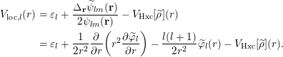 $$\begin{eqnarray}\displaystyle V_{\text{loc},l}(r) & = & \displaystyle \unicode[STIX]{x1D700}_{l}+\displaystyle \frac{\unicode[STIX]{x1D6E5}_{\mathbf{r}}\widetilde{\unicode[STIX]{x1D713}}_{lm}(\mathbf{r})}{2\unicode[STIX]{x1D713}_{lm}(\mathbf{r})}-V_{\text{Hxc}}[\widetilde{\unicode[STIX]{x1D70C}}](r)\nonumber\\ \displaystyle & = & \displaystyle \unicode[STIX]{x1D700}_{l}+\displaystyle \frac{1}{2r^{2}}\displaystyle \frac{\unicode[STIX]{x2202}}{\unicode[STIX]{x2202}r}\biggl(r^{2}\displaystyle \frac{\unicode[STIX]{x2202}\widetilde{\unicode[STIX]{x1D711}}_{l}}{\unicode[STIX]{x2202}r}\biggr)-\displaystyle \frac{l(l+1)}{2r^{2}}\widetilde{\unicode[STIX]{x1D711}}_{l}(r)-V_{\text{Hxc}}[\widetilde{\unicode[STIX]{x1D70C}}](r).\end{eqnarray}$$
Due to the spherical symmetry,
 $\unicode[STIX]{x1D700}_{l}$
,
 $V_{\text{loc},l}$
depend only on
 $l$
but not on
 $m$
. Again,
 $V_{\text{loc},l}(r)$
is only a function of the radial distance
 $r$
. Clearly
 $V_{\text{ps}}$
cannot be equal to
 $V_{\text{loc},l}(r)$
for all different choices of
 $l$
.
Below we demonstrate that HSC condition (1) can be satisfied if we allow
 $V_{\text{ps}}$
to be a non-local potential, i.e. an integral operator. We first choose the local potential to be
 $V_{\text{loc},l_{0}}$
for a particular angular momentum
 $l_{0}$
. Then let the kernel of
 $V_{\text{ps}}$
take the following form:
 $$\begin{eqnarray}V_{\text{ps}}(\mathbf{r},\mathbf{r}^{\prime })=V_{\text{loc},l_{0}}(r)\unicode[STIX]{x1D6FF}_{\mathbf{r},\mathbf{r}^{\prime }}+\mathop{\sum }_{lm}Y_{lm}(\hat{\mathbf{r}})(V_{\text{loc},l}(r)-V_{\text{loc},l_{0}}(r))\unicode[STIX]{x1D6FF}_{r,r^{\prime }}Y_{lm}^{\ast }(\hat{\mathbf{r}}^{\prime })/r^{2}.\end{eqnarray}$$
Applying equation (2.80) to a pseudo-valence orbital
 $\widetilde{\unicode[STIX]{x1D713}}_{lm}$
, we have
 $$\begin{eqnarray}\displaystyle (V_{\text{ps}}\widetilde{\unicode[STIX]{x1D713}}_{lm})(\mathbf{r}) & = & \displaystyle \int V_{\text{ps}}(\mathbf{r},\mathbf{r}^{\prime })\widetilde{\unicode[STIX]{x1D713}}_{lm}(\mathbf{r}^{\prime })\,\text{d}\mathbf{r}^{\prime }\nonumber\\ \displaystyle & = & \displaystyle V_{\text{loc},l_{0}}(r)\widetilde{\unicode[STIX]{x1D713}}_{lm}(\mathbf{r})+Y_{lm}(\hat{\mathbf{r}})(V_{\text{loc},l}(r)-V_{\text{loc},l_{0}}(r))\widetilde{\unicode[STIX]{x1D711}}_{l}(r)\nonumber\\ \displaystyle & = & \displaystyle V_{\text{loc},l}(r)\widetilde{\unicode[STIX]{x1D713}}_{lm}(\mathbf{r}).\end{eqnarray}$$
Here we have used the form (2.77) and the orthonormality condition of spherical harmonics. Combined with equation (2.79), we find that HSC condition (1) is satisfied for any valence orbital
 $\widetilde{\unicode[STIX]{x1D713}}_{lm}$
under consideration.
Since the kernel of
 $V_{\text{ps}}$
is local with respect to the radial variable, and non-local with respect to angular variables, equation (2.80) is called the semi-local form of the pseudopotential. However, for a general atomic configuration, the semi-local form cannot be treated efficiently other than being discretized as a dense matrix. Therefore the semi-local pseudopotential is rarely used in practice. In order to reduce the computational cost, we may note that it is only necessary for equation (2.81) to hold. Define
 $$\begin{eqnarray}\unicode[STIX]{x1D6FF}V_{\text{loc},l}(r):=V_{\text{loc},l}(r)-V_{\text{loc},l_{0}}(r).\end{eqnarray}$$
We note that
 $$\begin{eqnarray}\displaystyle \langle \unicode[STIX]{x1D6FF}V_{\text{loc},l}\widetilde{\unicode[STIX]{x1D713}}_{lm}|\widetilde{\unicode[STIX]{x1D713}}_{l^{\prime }m^{\prime }}\rangle & = & \displaystyle \int \unicode[STIX]{x1D6FF}V_{\text{loc},l}(r)\widetilde{\unicode[STIX]{x1D711}}_{l}^{\ast }(r)\widetilde{\unicode[STIX]{x1D711}}_{l^{\prime }}(r)Y_{lm}^{\ast }(\hat{\mathbf{r}})Y_{l^{\prime }m^{\prime }}(\hat{\mathbf{r}})\,\text{d}\mathbf{r}\nonumber\\ \displaystyle & = & \displaystyle \unicode[STIX]{x1D6FF}_{ll^{\prime }}\unicode[STIX]{x1D6FF}_{mm^{\prime }}\int _{0}^{\infty }r^{2}\unicode[STIX]{x1D6FF}V_{\text{loc},l}(r)|\widetilde{\unicode[STIX]{x1D711}}_{l}(r)|^{2}\,\text{d}r.\end{eqnarray}$$
Here we have used the orthonormality condition of the spherical harmonics. Now define the pseudopotential as
 $$\begin{eqnarray}V_{\text{ps}}=V_{\text{loc},l_{0}}+\mathop{\sum }_{lm}\displaystyle \frac{1}{\langle \unicode[STIX]{x1D6FF}V_{\text{loc},l}\widetilde{\unicode[STIX]{x1D713}}_{lm}|\widetilde{\unicode[STIX]{x1D713}}_{lm}\rangle }|\unicode[STIX]{x1D6FF}V_{\text{loc},l}\widetilde{\unicode[STIX]{x1D713}}_{lm}\rangle \langle \unicode[STIX]{x1D6FF}V_{\text{loc},l}\widetilde{\unicode[STIX]{x1D713}}_{lm}|.\end{eqnarray}$$
We may readily verify that
 $$\begin{eqnarray}V_{\text{ps}}\widetilde{\unicode[STIX]{x1D713}}_{lm}=V_{\text{loc},l_{0}}\widetilde{\unicode[STIX]{x1D713}}_{lm}+\unicode[STIX]{x1D6FF}V_{\text{loc},l}\widetilde{\unicode[STIX]{x1D713}}_{lm}=V_{\text{loc},l}\widetilde{\unicode[STIX]{x1D713}}_{lm},\end{eqnarray}$$
which means that
 $V_{\text{ps}}$
also satisfies HSC condition (1). Compared to the semi-local form, the pseudopotential (2.84) consists of a local component, as well as a non-local component that can be stored as a low-rank matrix. The rank is equal to the number of pseudo-valence orbitals under consideration. This is called the Kleinman–Bylander form of non-local pseudopotential (Kleinman and Bylander Reference Kleinman and Bylander1982), and is used in almost all modern electronic structure software packages using norm-conserving pseudopotentials.
Let us define
 $$\begin{eqnarray}b_{lm}(\mathbf{r})=\displaystyle \frac{1}{\sqrt{|\langle \unicode[STIX]{x1D6FF}V_{\text{loc},l}\widetilde{\unicode[STIX]{x1D713}}_{lm}|\widetilde{\unicode[STIX]{x1D713}}_{lm}\rangle |}}\unicode[STIX]{x1D6FF}V_{\text{loc}}(r)\widetilde{\unicode[STIX]{x1D711}}_{l}(r)Y_{lm}(\hat{\mathbf{r}}),\end{eqnarray}$$
which is called a projection vector. From HSC condition (2) and equation (2.79), we may readily find that
 $b_{lm}(\mathbf{r})=0$
if
 $r\geq r_{c}$
, and hence is localized in real space. Defining
 $\unicode[STIX]{x1D6FE}_{l}=\text{sign}(\langle \unicode[STIX]{x1D6FF}V_{\text{loc},l}\widetilde{\unicode[STIX]{x1D713}}_{lm}|\widetilde{\unicode[STIX]{x1D713}}_{lm}\rangle )$
and
 $V_{\text{loc}}(\mathbf{r}):=V_{\text{loc},l_{0}}(r)$
, we may rewrite the kernel of the Kleinman–Bylander form as
 $$\begin{eqnarray}V_{\text{ps}}(\mathbf{r},\mathbf{r}^{\prime })=V_{\text{loc}}(\mathbf{r})\unicode[STIX]{x1D6FF}_{\mathbf{r},\mathbf{r}^{\prime }}+\mathop{\sum }_{lm}\unicode[STIX]{x1D6FE}_{l}b_{lm}(\mathbf{r})b_{lm}^{\ast }(\mathbf{r}^{\prime }).\end{eqnarray}$$
Finally, the pseudopotential (2.87) only comes from one atom centred at the origin. For a general atomic configuration
 $\{\mathbf{R}_{I}\}_{I=1}^{M}$
, the kernel of the non-local pseudopotential takes the form
 $$\begin{eqnarray}\displaystyle V_{\text{ps}}(\mathbf{r},\mathbf{r}^{\prime };\{\mathbf{R}_{I}\}) & = & \displaystyle \Bigg\{\mathop{\sum }_{I=1}^{M}V_{\text{loc},I}(\mathbf{r}-\mathbf{R}_{I})\Bigg\}\unicode[STIX]{x1D6FF}_{\mathbf{r},\mathbf{r}^{\prime }}\nonumber\\ \displaystyle & & \displaystyle \qquad +\Bigg\{\mathop{\sum }_{I=1}^{M}\mathop{\sum }_{\ell =1}^{L_{I}}\unicode[STIX]{x1D6FE}_{\ell ,I}b_{\ell ,I}(\mathbf{r}-\mathbf{R}_{I})b_{\ell ,I}^{\ast }(\mathbf{r}^{\prime }-\mathbf{R}_{I})\Bigg\}\nonumber\\ \displaystyle & = & \displaystyle V_{\text{loc}}(\mathbf{r};\{\mathbf{R}_{I}\})\unicode[STIX]{x1D6FF}_{\mathbf{r},\mathbf{r}^{\prime }}+V_{\text{nl}}(\mathbf{r},\mathbf{r}^{\prime };\{\mathbf{R}_{I}\}).\end{eqnarray}$$
Here we have combined
 $lm$
into a multi-index
 $\ell$
. Furthermore,
 $V_{\text{loc},I},b_{\ell ,I}$
and the number of projection vectors
 $L_{I}$
depend on the atom type and hence have the added index
 $I$
. In this notation,
 $V_{\text{loc}}$
and
 $V_{\text{nl}}$
denote the collection of local and non-local parts of the pseudopotential, respectively. Equation (2.88) is the general form of norm-conserving pseudopotential and will be assumed throughout this review.
More explicitly, the Kohn–Sham energy under the pseudopotential approximation becomes
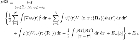 $$\begin{eqnarray}\displaystyle & & \displaystyle E^{\text{KS}}=\inf _{\{\unicode[STIX]{x1D713}_{i}\}_{i=1}^{N},\langle \unicode[STIX]{x1D713}_{i}|\unicode[STIX]{x1D713}_{j}\rangle =\unicode[STIX]{x1D6FF}_{ij}}\nonumber\\ \displaystyle & & \displaystyle \quad \Bigg\{\displaystyle \frac{1}{2}\mathop{\sum }_{i=1}^{N}\int |\unicode[STIX]{x1D6FB}\unicode[STIX]{x1D713}_{i}(\mathbf{r})|^{2}\,\text{d}\mathbf{r}+\mathop{\sum }_{i=1}^{N}\int \unicode[STIX]{x1D713}_{i}^{\ast }(\mathbf{r})V_{\text{nl}}(\mathbf{r},\mathbf{r}^{\prime };\{\mathbf{R}_{I}\})\unicode[STIX]{x1D713}_{i}(\mathbf{r}^{\prime })\,\text{d}\mathbf{r}\,\text{d}\mathbf{r}^{\prime }\nonumber\\ \displaystyle & & \displaystyle \quad \qquad +\int \unicode[STIX]{x1D70C}(\mathbf{r})V_{\text{loc}}(\mathbf{r};\{\mathbf{R}_{I}\})\,\text{d}\mathbf{r}+\displaystyle \frac{1}{2}\int \displaystyle \frac{\unicode[STIX]{x1D70C}(\mathbf{r})\unicode[STIX]{x1D70C}(\mathbf{r}^{\prime })}{|\mathbf{r}-\mathbf{r}^{\prime }|}\,\text{d}\mathbf{r}\,\text{d}\mathbf{r}^{\prime }+E_{\text{xc}}[\unicode[STIX]{x1D70C}]\Bigg\}+E_{\text{II}}.\end{eqnarray}$$
The corresponding Kohn–Sham Hamiltonian becomes
 $$\begin{eqnarray}H^{\text{KS}}[\unicode[STIX]{x1D70C}]=-\displaystyle \frac{1}{2}\unicode[STIX]{x1D6E5}+V_{\text{loc}}+V_{\text{nl}}+V_{H}[\unicode[STIX]{x1D70C}]+V_{\text{xc}}[\unicode[STIX]{x1D70C}].\end{eqnarray}$$
When the electron density is given, the effective potential (2.33) becomes
 $$\begin{eqnarray}V_{\text{eff}}(\mathbf{r})=V_{\text{loc}}(\mathbf{r})+V_{H}[\unicode[STIX]{x1D70C}](\mathbf{r})+V_{\text{xc}}[\unicode[STIX]{x1D70C}](\mathbf{r}),\end{eqnarray}$$
where we have separated out the contribution from the non-local pseudo- potential
 $V_{\text{nl}}$
.
Remarks
Although not discussed here, another major reason for using pseudopotential is to take into account relativistic effects, which are non-negligible for heavy elements such as lead and gold. Since relativistic effects mainly affect the behaviour of core electrons, we may solve the relativistic Dirac–Kohn–Sham equation (Thaller Reference Thaller1992, Belpassi, Tarantelli, Sgamellotti and Quiney Reference Belpassi, Tarantelli, Sgamellotti and Quiney2005) for a single atom to obtain the relativistically corrected valence orbitals
 $\unicode[STIX]{x1D713}_{lm}$
and energies
 $\unicode[STIX]{x1D700}_{l}$
. The rest of the procedure for generating the pseudopotential is the same as above.
There are a number of widely used norm-conserving pseudopotentials, such as the Troullier–Martins (TM) pseudopotential (Troullier and Martins Reference Troullier and Martins1991), the Hartwigsen–Goedecker–Hutter (HGH) pseudopotential (Hartwigsen, Goedecker and Hutter Reference Hartwigsen, Goedecker and Hutter1998) and the optimized norm-conserving Vanderbilt (ONCV) pseudopotential (Hamann Reference Hamann2013), to name just a few. All these pseudopotentials can be written in the form (2.88), though the interpretation of
 $V_{\text{loc}},b_{\ell }$
and even the number of projectors
 $L$
may be different. Recently the semi-local form of the pseudopotential has been analysed mathematically (Cancès and Mourad Reference Cancès and Mourad2016). However, the Kleinman–Bylander form of pseudopotential may occasionally introduce ‘ghost states’, which are unphysical states with artificially low energies. In practice such ghost states can often be removed by choosing the local potential to have a different angular momentum
 $l$
, and hence they are often not considered to be a problem in most electronic structure calculations. However, the existence of ghost states introduces difficulty into the mathematical analysis.
It may appear that the norm-conservation condition should be naturally imposed since the pseudo-valence orbitals
 $\widetilde{\unicode[STIX]{x1D713}}_{lm}$
should be eigenfunctions of a modified Schrödinger operator. However, it has been found that by relaxing the norm-conservation condition, one can further improve the smoothness of the pseudopotential and hence reduce the computational cost. The most well-known example is the Vanderbilt ultrasoft pseudopotential (Vanderbilt Reference Vanderbilt1990). Moreover, the widely used projected augmented wave (PAW) method (Blöchl Reference Blöchl1994) can also be viewed as a pseudopotential, which also violates the norm-conservation condition. Compared to norm-conserving pseudopotentials, one drawback of such approaches is that the Kohn–Sham equations become inherently a generalized eigenvalue problem even when the basis set is orthonormal (see Section 3).
2.8 Physical quantities of interest
Once the Kohn–Sham equations have converged, the total energy can be evaluated readily from equation (2.89). It can also be evaluated from the Kohn–Sham eigenvalues as
 $$\begin{eqnarray}E^{\text{KS}}=\mathop{\sum }_{i=1}^{N}\unicode[STIX]{x1D700}_{i}-\displaystyle \frac{1}{2}\int \displaystyle \frac{\unicode[STIX]{x1D70C}(\mathbf{r})\unicode[STIX]{x1D70C}(\mathbf{r}^{\prime })}{|\mathbf{r}-\mathbf{r}^{\prime }|}\,\text{d}\mathbf{r}\,\text{d}\mathbf{r}^{\prime }-\int \unicode[STIX]{x1D70C}(\mathbf{r})V_{\text{xc}}[\unicode[STIX]{x1D70C}](\mathbf{r})\,\text{d}\mathbf{r}+E_{\text{xc}}[\unicode[STIX]{x1D70C}]+E_{\text{II}}.\end{eqnarray}$$
Here the summation of the eigenvalues
 $\sum _{i=1}^{N}\unicode[STIX]{x1D700}_{i}$
is called the band energy. The difference between the total energy and the band energy (other than the nuclei interaction energy
 $E_{\text{II}}$
) is called the double-counting term, which is due to the nonlinearity of the Hartree energy and the exchange-correlation energy functionals. When finite temperature effects are included, the entropy also needs to be evaluated in order to compute the free energy.
In Kohn–Sham DFT, besides the total energy and the electron density, we are often interested in computing the atomic force, which is necessary for performing geometry relaxation and ab initio molecular dynamics simulation. Once the SCF iteration reaches convergence, the force on the
 $I$
th atom can be computed as the negative derivative of the total energy with respect to the atomic position
 $\mathbf{R}_{I}$
:
 $$\begin{eqnarray}\mathbf{F}_{I}=-\displaystyle \frac{\unicode[STIX]{x2202}E^{\text{KS}}(\{\mathbf{R}_{I}\})}{\unicode[STIX]{x2202}\mathbf{R}_{I}}.\end{eqnarray}$$
The required derivative can be computed directly, for examplevia finite differences. However, even for first-order accuracy, the number of energy evaluations for a system containing
 $M$
atoms is
 $3M+1$
, that is, the Kohn–Sham equations must be solved
 $3M+1$
times independently. This approach becomes prohibitively expensive as the system size increases. The cost of the force calculation is greatly reduced via the Hellmann–Feynman theorem (Martin Reference Martin2008), which states that, at self-consistency, the partial derivative
 $\unicode[STIX]{x2202}/\unicode[STIX]{x2202}\mathbf{R}_{I}$
only needs to be applied to terms in equation (2.89) which depend explicitly on the atomic position
 $\mathbf{R}_{I}$
. The Hellmann–Feynman (HF) force is then given by
 $$\begin{eqnarray}\displaystyle \mathbf{F}_{I} & = & \displaystyle -\int \displaystyle \frac{\unicode[STIX]{x2202}V_{\text{loc}}}{\unicode[STIX]{x2202}\mathbf{R}_{I}}(\mathbf{r};\{\mathbf{R}_{I}\})\unicode[STIX]{x1D70C}(\mathbf{r})\,\text{d}\mathbf{r}-\mathop{\sum }_{i=1}^{N}\int \unicode[STIX]{x1D713}_{i}^{\ast }(\mathbf{r})\displaystyle \frac{\unicode[STIX]{x2202}V_{\text{nl}}}{\unicode[STIX]{x2202}\mathbf{R}_{I}}(\mathbf{r},\mathbf{r}^{\prime };\{\mathbf{R}_{I}\})\unicode[STIX]{x1D713}_{i}(\mathbf{r}^{\prime })\,\text{d}\mathbf{r}\,\text{d}\mathbf{r}^{\prime }\nonumber\\ \displaystyle & & \displaystyle +\mathop{\sum }_{J\neq I}\displaystyle \frac{Z_{I}Z_{J}}{|\mathbf{R}_{I}-\mathbf{R}_{J}|^{3}}(\mathbf{R}_{I}-\mathbf{R}_{J}).\end{eqnarray}$$
Note that equation (2.88) gives
 $$\begin{eqnarray}\displaystyle \frac{\unicode[STIX]{x2202}V_{\text{loc}}}{\unicode[STIX]{x2202}\mathbf{R}_{I}}(\mathbf{r};\{\mathbf{R}_{I}\})=\displaystyle \frac{\unicode[STIX]{x2202}V_{\text{loc},I}}{\unicode[STIX]{x2202}\mathbf{R}_{I}}(\mathbf{r}-\mathbf{R}_{I})=-\unicode[STIX]{x1D6FB}_{\mathbf{r}}V_{\text{loc},I}(\mathbf{r}-\mathbf{R}_{I}),\end{eqnarray}$$
and
 $$\begin{eqnarray}\displaystyle & & \displaystyle \displaystyle \frac{\unicode[STIX]{x2202}V_{\text{nl}}}{\unicode[STIX]{x2202}\mathbf{R}_{I}}(\mathbf{r},\mathbf{r}^{\prime };\{\mathbf{R}_{I}\})\nonumber\\ \displaystyle & & \displaystyle \quad =\mathop{\sum }_{\ell =1}^{L_{I}}\unicode[STIX]{x1D6FE}_{I,\ell }\biggl(\displaystyle \frac{\unicode[STIX]{x2202}b_{I,\ell }}{\unicode[STIX]{x2202}\mathbf{R}_{I}}(\mathbf{r}-\mathbf{R}_{I})b_{I,\ell }^{\ast }(\mathbf{r}^{\prime }-\mathbf{R}_{I})+b_{I,\ell }(\mathbf{r}-\mathbf{R}_{I})\displaystyle \frac{\unicode[STIX]{x2202}b_{I,\ell }^{\ast }}{\unicode[STIX]{x2202}\mathbf{R}_{I}}(\mathbf{r}^{\prime }-\mathbf{R}_{I})\biggr)\nonumber\\ \displaystyle & & \displaystyle \quad =-\mathop{\sum }_{\ell =1}^{L_{I}}\unicode[STIX]{x1D6FE}_{I,\ell }(\unicode[STIX]{x1D6FB}_{\mathbf{r}}b_{I,\ell }(\mathbf{r}-\mathbf{R}_{I})b_{I,\ell }^{\ast }(\mathbf{r}^{\prime }-\mathbf{R}_{I})+b_{I,\ell }(\mathbf{r}-\mathbf{R}_{I})\unicode[STIX]{x1D6FB}_{\mathbf{r}^{\prime }}b_{I,\ell }^{\ast }(\mathbf{r}^{\prime }-\mathbf{R}_{I})).\nonumber\end{eqnarray}$$
Then the Hellmann–Feynman force in equation (2.94) can be written as
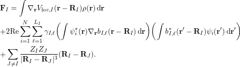 $$\begin{eqnarray}\displaystyle & & \displaystyle \mathbf{F}_{I}=\int \unicode[STIX]{x1D6FB}_{\mathbf{r}}V_{\text{loc},I}(\mathbf{r}-\mathbf{R}_{I})\unicode[STIX]{x1D70C}(\mathbf{r})\,\text{d}\mathbf{r}\nonumber\\ \displaystyle & & \displaystyle +2\text{Re}\mathop{\sum }_{i=1}^{N}\mathop{\sum }_{\ell =1}^{L_{I}}\unicode[STIX]{x1D6FE}_{I,\ell }\biggl(\int \unicode[STIX]{x1D713}_{i}^{\ast }(\mathbf{r})\unicode[STIX]{x1D6FB}_{\mathbf{r}}b_{I,\ell }(\mathbf{r}-\mathbf{R}_{I})\,\text{d}\mathbf{r}\biggr)\biggl(\int b_{I,\ell }^{\ast }(\mathbf{r}^{\prime }-\mathbf{R}_{I})\unicode[STIX]{x1D713}_{i}(\mathbf{r}^{\prime })\,\text{d}\mathbf{r}^{\prime }\biggr)\nonumber\\ \displaystyle & & \displaystyle +\mathop{\sum }_{J\neq I}\displaystyle \frac{Z_{I}Z_{J}}{|\mathbf{R}_{I}-\mathbf{R}_{J}|^{3}}(\mathbf{R}_{I}-\mathbf{R}_{J}).\end{eqnarray}$$
From the computational cost point of view, if we let
 $N_{g}$
denote the number of grid points to discretize quantities such as
 $\unicode[STIX]{x1D70C}(\mathbf{r})$
in the global domain to perform a quadrature, then the cost of computing the force due to the local potential
 $\int \unicode[STIX]{x1D6FB}_{\mathbf{r}}V_{\text{loc},I}(\mathbf{r}-\mathbf{R}_{I})\unicode[STIX]{x1D70C}(\mathbf{r})\,\text{d}\mathbf{r}$
is
 $O(N_{g})$
, since
 $V_{\text{loc},I}(\mathbf{r}-\mathbf{R}_{I})$
is a delocalized quantity in the global domain. On the other hand, each non-local projector
 $b_{I,\ell }(\mathbf{r}-\mathbf{R}_{I})$
is localized around
 $\mathbf{R}_{I}$
, and the cost of evaluating the integral
 $(\int \unicode[STIX]{x1D713}_{i}^{\ast }(\mathbf{r})\unicode[STIX]{x1D6FB}_{\mathbf{r}}b_{I,\ell }(\mathbf{r}-\mathbf{R}_{I})\,\text{d}\mathbf{r})$
or
 $(\int b_{I,\ell }^{\ast }(\mathbf{r}^{\prime }-\mathbf{R}_{I})\unicode[STIX]{x1D713}_{i}(\mathbf{r}^{\prime })\,\text{d}\mathbf{r}^{\prime })$
is a constant
 $N_{l}$
independent of the global number of grid points
 $N_{g}$
. The computation of the last term,
 $$\begin{eqnarray}\mathop{\sum }_{J\neq I}\displaystyle \frac{Z_{I}Z_{J}}{|\mathbf{R}_{I}-\mathbf{R}_{J}|^{3}}(\mathbf{R}_{I}-\mathbf{R}_{J}),\end{eqnarray}$$
involves only scalar operations, and its cost is usually negligibly small in electronic structure calculations.
 $N_{g}$
and
 $N_{I}$
are proportional to the number of electrons
 $N$
. Hence, neglecting constant terms independent of
 $N$
, we have that the computational cost of the Hellmann–Feynman force on each atom is
 $O(N_{g}+NL_{I}N_{l})\sim O(N)$
, and the cost of computing forces on all atoms is
 $O(N^{2})$
.
Remarks
The computational cost of evaluating equation (2.95) can scale as
 $O(N^{3})$
if implemented straightforwardly. This is because, for each atom, the associated non-local pseudopotential needs to be applied to all orbitals via an integral. The cost is thus
 $MNN_{g}\sim O(N^{3})$
. Note that each projection vector
 $b_{\ell ,I}$
has (at least approximately) compact support in real space and can thus be stored as a sparse vector, using the real-space representation (see Section 3.1.2). The number of non-zeros in the sparse vector is independent of the number of quadrature points in the global domain. The cost is then reduced to
 $O(N^{2})$
as discussed above. We remark that use of the real-space representation may result in higher numerical error than the Fourier space representation (see Section 3.1.1), especially if the real-space grid is not dense enough. Hence several electronic structure software packages such as Quantum ESPRESSO still prefer the Fourier space representation, even though the cost scales as
 $O(N^{3})$
. In certain contexts, the computational cost can be further reduced to
 $O(N)$
using density matrix formalism (see Section 3.3).
The atomic force evaluated as in equation (2.95) uses the Hellmann–Feynman theorem, and hence is called the Hellmann–Feynman force. When numerical discretization as in Section 3 is under consideration, the derivative of the Kohn–Sham energy may involve the derivative with respect to a basis function. If the basis set depends on the atomic configuration, such as in the case of Gaussian-type orbitals to be discussed in Section 3.2, then the Hellmann–Feynman force does not agree with the negative derivative of the Kohn–Sham energy. The remaining difference is called the Pulay force (Pulay Reference Pulay1969). On the other hand, if the discretization is independent of atomic configuration, such as in the case of the planewave basis set in Section 3.1, the Pulay force vanishes and the Hellmann–Feynman force becomes exact. We also remark that even if the basis set depends on the atomic configuration, the magnitude of the Pulay force will systematically decrease as the basis set approaches the complete basis set limit.
3 Numerical discretization
In order to solve Kohn–Sham DFT in practice, the Hamiltonian operator must first be discretized, for instance by a finite-sized basis set. The efficiency of a discretization scheme can be measured in terms of the number of degrees of freedom per atom, or the dimension of the discretized Hamiltonian matrix. Besides this standard metric, one special feature of electronic structure calculations is that the choice of the discretization scheme can directly affect the effectiveness of subsequent numerical methods to evaluate the Kohn–Sham map, which is to be discussed in detail in Sections 5 and 6. In the following discussion, we divide the numerical discretization schemes roughly into three categories: large basis sets (Section 3.1), small basis sets (Section 3.2) and adaptive basis sets (Section 3.3).
3.1 Large basis sets
In electronic structure calculations, a large basis set typically requires
 $100\sim 10\,000$
basis functions per atom to achieve chemical accuracy, even when pseudopotentials are used. The size of the resulting Hamiltonian matrix is usually of the order of
 $10^{3}\sim 10^{6}$
. Hence it is not numerically efficient, or even feasible at all, to diagonalize the Hamiltonian matrix. In such a case, iterative algorithms should be used to compute the occupied orbitals, which will be discussed in Section 4.2. Most standard basis sets used to solve PDEs numerically fall into this category, for instance the planewave method (Payne et al.
Reference Payne, Teter, Allen, Arias and Joannopoulos1992, Kresse and Furthmüller Reference Kresse and Furthmüller1996) (also known as the Fourier basis set, or more precisely, the pseudospectral method), the finite element method (Tsuchida and Tsukada Reference Tsuchida and Tsukada1995, Suryanarayana et al.
Reference Suryanarayana, Gavani, Blesgen, Bhattacharya and Ortiz2010, Bao, Hu and Liu Reference Bao, Hu and Liu2012, Chen et al.
Reference Chen, Dai, Gong, He and Zhou2014) and the wavelet method (Genovese et al.
Reference Genovese, Neelov, Goedecker, Deutsch, Ghasemi, Willand, Caliste, Zilberberg, Rayson, Bergman and Schneider2008), to name just a few. Strictly speaking, the finite difference method (Chelikowsky, Troullier and Saad Reference Chelikowsky, Troullier and Saad1994) does not use a basis set. However, the number of degrees of freedom needed by the finite difference method is approximately in the same range, and hence finite difference can also be regarded as a large basis set method. The main advantage of using a large basis set is that physical quantities such as energies and forces can converge systematically with respect to refinement of the basis set, by tuning one or a few parameters.
3.1.1 Fourier basis set
For charge-neutral systems, periodic boundary conditions are often sufficiently accurate when the Coulomb energy is treated with care (Makov and Payne Reference Makov and Payne1995). One of the key advantages of working with periodic boundary conditions is that they allow use of the Fourier basis set, which is arguably the most widely used large basis set for electronic structure calculations. In the Fourier basis set, the basis functions are of the form
 $\exp (\text{i}\mathbf{g}\cdot \mathbf{r})$
, where the parameter
 $\mathbf{g}$
is chosen from a specific set of frequencies. The Fourier basis set has several key advantages. First, the discretization of the Kohn–Sham Hamiltonian takes a rather simple form under this basis set. Second, as it is independent of the atom configurations, the Pulay force vanishes, thus making the force calculation rather straightforward. Third, by leveraging the fast Fourier transform (FFT), computation of the matrix–vector multiplication with the Kohn–Sham Hamiltonian can be carried out efficiently, and this allows for efficient iterative diagonalization while evaluating the Kohn–Sham map. However, the Fourier basis set also comes with a noticeable disadvantage: as a fixed basis set, it lacks the flexibility of local refinement, which can be a serious issue for all-electron calculations. Fortunately, introduction of the pseudopotentials addresses this problem by eliminating the singularity at the nuclei, as well as the highly localized core electrons. This allows one to focus solely on the smooth valence electrons. In the rest of this subsection, we shall work with the Kohn–Sham Hamiltonian under the pseudopotentials approximation as in equation (2.90).
Let us consider for simplicity a rectangular computational domain
 $\unicode[STIX]{x1D6FA}=[0,L_{1}]\times [0,L_{2}]\times [0,L_{3}]$
with periodic boundary conditions. It is natural to associate with
 $\unicode[STIX]{x1D6FA}$
a reciprocal lattice in frequency space given by
 $$\begin{eqnarray}\mathbb{L}^{\ast }=\bigg\{\mathbf{g}=\bigg(\displaystyle \frac{2\unicode[STIX]{x1D70B}}{L_{1}}i_{1},\displaystyle \frac{2\unicode[STIX]{x1D70B}}{L_{2}}i_{2},\displaystyle \frac{2\unicode[STIX]{x1D70B}}{L_{3}}i_{3}\bigg)\;:\;(i_{1},i_{2},i_{3})\in \mathbb{Z}^{3}\bigg\},\end{eqnarray}$$
and the Fourier basis functions are the complex exponentials
 $$\begin{eqnarray}\unicode[STIX]{x1D719}_{\mathbf{g}}(\mathbf{r})=\displaystyle \frac{1}{\sqrt{|\unicode[STIX]{x1D6FA}|}}\exp (\text{i}\mathbf{g}\cdot \mathbf{r})\end{eqnarray}$$
indexed by each
 $\mathbf{g}\in \mathbb{L}^{\ast }$
. In order to obtain a finite set of basis functions, one typically introduces an energy cut-off
 $E_{\text{cut}}$
and restricts to only the Fourier modes indexed by
 $$\begin{eqnarray}\mathbb{G}_{\text{cut}}:=\bigg\{\mathbf{g}\in \mathbb{L}^{\ast }:\displaystyle \frac{1}{2}|\mathbf{g}|^{2}\leq E_{\text{cut}}\bigg\}\subset \mathbb{L}^{\ast }.\end{eqnarray}$$
We will use
 $N_{b}$
to denote the cardinality of
 $\mathbb{G}_{\text{cut}}$
, i.e. the number of basis functions used within the energy cut-off.
In order to present the Kohn–Sham Hamiltonian under this basis, it is convenient to introduce two Cartesian grids, one in frequency space and one in real space. The one in frequency space is
 $$\begin{eqnarray}\displaystyle \mathbb{G} & = & \displaystyle \bigg\{\mathbf{g}=\bigg(\displaystyle \frac{2\unicode[STIX]{x1D70B}}{L_{1}}i_{1},\displaystyle \frac{2\unicode[STIX]{x1D70B}}{L_{2}}i_{2},\displaystyle \frac{2\unicode[STIX]{x1D70B}}{L_{3}}i_{3}\bigg)\;:\;\nonumber\\ \displaystyle & & \displaystyle \qquad -\displaystyle \frac{n_{1}}{2}\leq i_{1}<\displaystyle \frac{n_{1}}{2},-\displaystyle \frac{n_{2}}{2}\leq i_{2}<\displaystyle \frac{n_{2}}{2},-\displaystyle \frac{n_{3}}{2}\leq i_{3}<\displaystyle \frac{n_{3}}{2}\bigg\},\nonumber\end{eqnarray}$$
where
 $n_{1}$
,
 $n_{2}$
, and
 $n_{3}$
are chosen in such a way that the width of
 $\mathbb{G}$
in each dimension is typically twice the width of
 $\mathbb{G}_{\text{cut}}$
. The reason for such a choice will be discussed below. The Cartesian grid in real space is denoted by
 $$\begin{eqnarray}\mathbb{X}=\bigg\{\mathbf{r}=\biggl(\displaystyle \frac{i_{1}}{n_{1}}L_{1},\displaystyle \frac{i_{2}}{n_{2}}L_{2},\displaystyle \frac{i_{3}}{n_{3}}L_{3}\biggr):0\leq i_{1}<n_{1},0\leq i_{2}<n_{2},0\leq i_{3}<n_{3}\bigg\}.\end{eqnarray}$$
Note that the number of grid points in both grids is equal to
 $N_{g}=n_{1}n_{2}n_{3}$
.
For a function
 $\unicode[STIX]{x1D713}(\mathbf{r})$
in the span of
 $\{\unicode[STIX]{x1D719}_{\mathbf{g}}(\mathbf{r})\;:\;\mathbf{g}\in \mathbb{G}_{\text{cut}}\}$
with spanning coefficients
 $\{\hat{\unicode[STIX]{x1D713}}_{\mathbf{g}}\;:\;\mathbf{g}\in \mathbb{G}_{\text{cut}}\}$
, its value at any point
 $\mathbf{r}\in \mathbb{X}$
is given by
 $$\begin{eqnarray}\unicode[STIX]{x1D713}(\mathbf{r})=\mathop{\sum }_{\mathbf{g}\in \mathbb{G}_{\text{cut}}}\hat{\unicode[STIX]{x1D713}}_{\mathbf{g}}\unicode[STIX]{x1D719}_{\mathbf{g}}(\mathbf{r})=\mathop{\sum }_{\mathbf{g}\in \mathbb{G}_{\text{cut}}}\hat{\unicode[STIX]{x1D713}}_{\mathbf{g}}\displaystyle \frac{1}{\sqrt{|\unicode[STIX]{x1D6FA}|}}\exp (\text{i}\mathbf{g}\cdot \mathbf{r}).\end{eqnarray}$$
Suppose now that
 $\unicode[STIX]{x1D713}(\mathbf{r})$
is a sufficiently smooth function. Then the basis coefficients
 $\{\hat{\unicode[STIX]{x1D713}}_{\mathbf{g}}\;:\;\mathbf{g}\in \mathbb{G}\}$
can be approximated using the samples of
 $\unicode[STIX]{x1D713}(\mathbf{r})$
at
 $\mathbb{X}$
, computed via the inverse Fourier transform as
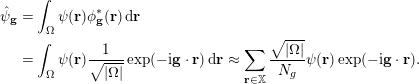 $$\begin{eqnarray}\displaystyle \hat{\unicode[STIX]{x1D713}}_{\mathbf{g}} & = & \displaystyle \int _{\unicode[STIX]{x1D6FA}}\unicode[STIX]{x1D713}(\mathbf{r})\unicode[STIX]{x1D719}_{\mathbf{g}}^{\ast }(\mathbf{r})\,\text{d}\mathbf{r}\nonumber\\ \displaystyle & = & \displaystyle \int _{\unicode[STIX]{x1D6FA}}\unicode[STIX]{x1D713}(\mathbf{r})\displaystyle \frac{1}{\sqrt{|\unicode[STIX]{x1D6FA}|}}\exp (-\text{i}\mathbf{g}\cdot \mathbf{r})\,\text{d}\mathbf{r}\approx \mathop{\sum }_{\mathbf{r}\in \mathbb{X}}\displaystyle \frac{\sqrt{|\unicode[STIX]{x1D6FA}|}}{N_{g}}\unicode[STIX]{x1D713}(\mathbf{r})\exp (-\text{i}\mathbf{g}\cdot \mathbf{r}).\end{eqnarray}$$
Note that the last approximation is exact if
 $\unicode[STIX]{x1D713}(\mathbf{r})$
belongs to the span of
 $\{\unicode[STIX]{x1D719}_{\mathbf{g}}(\mathbf{r})\;:\;\mathbf{g}\in \mathbb{G}_{\text{cut}}\}$
.
Illustration of the grids used for the Fourier basis set:
 $\mathbb{X}$
,
 $\mathbb{G}$
and
 $\mathbb{G}_{\text{cut}}$
.
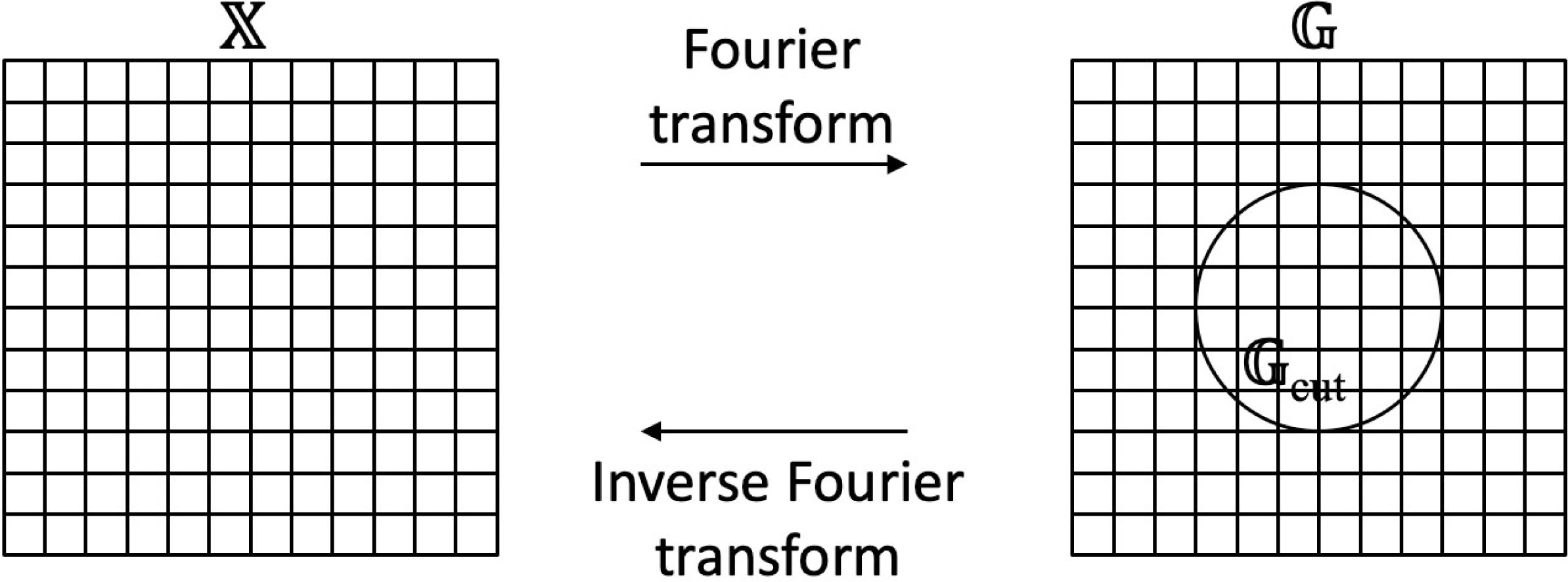
Equations (3.1) and (3.2) show how to transform between the real-space and frequency-space representations for a function
 $\unicode[STIX]{x1D713}(\mathbf{r})$
. Given the spanning coefficients
 $\{\hat{\unicode[STIX]{x1D713}}_{\mathbf{g}}\;:\;\mathbf{g}\in \mathbb{G}_{\text{cut}}\}$
, the values
 $\{\unicode[STIX]{x1D713}(\mathbf{r})\;:\;\mathbf{r}\in \mathbb{X}\}$
are computed by first extending
 $\hat{\unicode[STIX]{x1D713}}_{\mathbf{g}}$
from
 $\mathbb{G}_{\text{cut}}$
to
 $\mathbb{G}$
with zero-padding and then applying a discrete inverse Fourier transform. In the opposite direction, given the real-space values
 $\{\unicode[STIX]{x1D713}(\mathbf{r})\;:\;\mathbf{r}\in \mathbb{X}\}$
, the coefficients
 $\{\hat{\unicode[STIX]{x1D713}}_{\mathbf{g}}\;:\;\mathbf{g}\in \mathbb{G}_{\text{cut}}\}$
are computed by first applying a discrete Fourier transform and then restricting the result from
 $\mathbb{G}$
to
 $\mathbb{G}_{\text{cut}}$
. In terms of computational efficiency, it is essential that both directions can be accelerated using the fast Fourier transform. Figure 3.1 illustrates the grids involved in these conversions.
The Fourier basis set typically results in a dense matrix for the Kohn–Sham Hamiltonian in (2.89). Direct diagonalization of such dense matrices is often computationally too expensive. As a result, iterative diagonalization is often used instead (see Section 4.2). The key step of an iterative diagonalization algorithm is the application of the Kohn–Sham Hamiltonian to a given function represented in the Fourier basis set.
More precisely, for a function
 $\unicode[STIX]{x1D713}$
given in terms of its Fourier coefficients
 $\{\hat{\unicode[STIX]{x1D713}}_{\mathbf{g}}\;:\;\mathbf{g}\in \mathbb{G}_{\text{cut}}\}$
, the goal is to evaluate the Fourier coefficients of
 $H^{\text{KS}}\unicode[STIX]{x1D713}$
in
 $\mathbb{G}_{\text{cut}}$
effectively. Note from the definition (2.90) that the Kohn–Sham Hamiltonian
 $H^{\text{KS}}$
can be decomposed into three parts:
∙ the kinetic energy part
$-{\textstyle \frac{1}{2}}\unicode[STIX]{x1D6E5}$
,∙ the local potential part, that is,
where$$\begin{eqnarray}V_{\text{loc}}+V_{H}[\unicode[STIX]{x1D70C}]+V_{\text{xc}}[\unicode[STIX]{x1D70C}],\end{eqnarray}$$
$V_{\text{loc}}$
is the local part of the pseudopotential approximation,∙ the non-local part of the pseudopotential approximation
$V_{\text{nl}}$
.


The overall strategy is to treat each part individually, either in real space or in frequency space depending on computational convenience.
Before describing in detail how each of these three parts is treated, we note that the Kohn–Sham Hamiltonian depends on the electron density
 $\unicode[STIX]{x1D70C}(\cdot )$
. In the actual numerical computation, one needs access to the values of
 $\unicode[STIX]{x1D70C}(\cdot )$
at each
 $\mathbf{r}\in \mathbb{X}$
.
 $\unicode[STIX]{x1D70C}(\mathbf{r})$
is formed from the current copies of the Kohn–Sham orbitals
 $\{\unicode[STIX]{x1D713}_{i}(\mathbf{r})\}$
with
 $i=1,\ldots ,N$
. In the Fourier basis method,
 $\{\unicode[STIX]{x1D713}_{i}(\mathbf{r})\}$
are represented in the frequency domain
 $\hat{\unicode[STIX]{x1D713}}_{\mathbf{g};i}$
with
 $\mathbf{g}\in \mathbb{G}_{\text{cut}}$
. The computation of
 $\unicode[STIX]{x1D70C}(\mathbf{r})$
involves evaluating
 $\unicode[STIX]{x1D713}_{i}(\mathbf{r})$
for each
 $i$
(i.e. one fast Fourier transform), squaring them, and summing the results over
 $i=1,\ldots ,N$
. In order to avoid the aliasing error coming from the squaring step, it is typically required that the sidelength of
 $\mathbb{G}$
is significantly larger than the diameter of the grid
 $\mathbb{G}_{\text{cut}}$
(for details see e.g. Fornberg Reference Fornberg1998). In this case, the conventional choice in the electronic structure community is to set the sidelength of
 $\mathbb{G}$
to be at least twice the diameter of
 $\mathbb{G}_{\text{cut}}$
, as mentioned above.
With
 $\unicode[STIX]{x1D70C}(\mathbf{r})$
ready at each
 $\mathbf{r}\in \mathbb{X}$
, let us now go through each of the three parts when applying the Kohn–Sham Hamiltonian
 $H^{\text{KS}}$
to a function
 $\unicode[STIX]{x1D713}$
. First, consider the kinetic energy part
 $-{\textstyle \frac{1}{2}}\unicode[STIX]{x1D6E5}\unicode[STIX]{x1D713}$
. It is well known that a differential operator in real space is equivalent to a pointwise multiplication operator in frequency space. Therefore, applying the kinetic part
 $-{\textstyle \frac{1}{2}}\unicode[STIX]{x1D6E5}$
can be carried out by multiplying
 $\hat{\unicode[STIX]{x1D713}}_{\mathbf{g}}$
by
 ${\textstyle \frac{1}{2}}|\mathbf{g}|^{2}$
for each
 $\mathbf{g}\in \mathbb{G}_{\text{cut}}$
.
Second, for the computation of the local potential part, one first applies an inverse Fourier transform on
 $\{\hat{\unicode[STIX]{x1D713}}_{\mathbf{g}}\;:\;\mathbf{g}\in \mathbb{G}_{\text{cut}}\}$
to obtain the real-space representation
 $\{\unicode[STIX]{x1D713}(\mathbf{r})\;:\;\mathbf{r}\in \mathbb{X}\}$
. As mentioned above, the local potential consists of several parts,
 $$\begin{eqnarray}(V_{\text{loc}}(\mathbf{r})+V_{H}[\unicode[STIX]{x1D70C}](\mathbf{r})+V_{\text{xc}}[\unicode[STIX]{x1D70C}](\mathbf{r}))\unicode[STIX]{x1D713}(\mathbf{r}),\end{eqnarray}$$
The Hartree potential involves convolution in real space, and therefore it is convenient to treat it in the Fourier domain. More precisely, one first applies the Fourier transform to the electron density
 $\unicode[STIX]{x1D70C}(\mathbf{r})$
with
 $\mathbf{r}\in \mathbb{X}$
to obtain
 $\{\widehat{\unicode[STIX]{x1D70C}}_{\mathbf{g}}\;:\;\mathbf{g}\in \mathbb{G}_{\text{cut}}\}$
. Then each
 $\widehat{\unicode[STIX]{x1D70C}}_{\mathbf{g}}$
is multiplied by
 $1/|\mathbf{g}|^{2}$
, except that at
 $\mathbf{g}=0$
it is kept at zero. This is due to the charge neutrality assumption, which allows the formally divergent contribution from the Fourier mode
 $\mathbf{g}=0$
to be cancelled by the contribution from the electron–ion interaction. Finally, an inverse Fourier transform brings the result back to real space. When all the parts are ready, we compute the sum and multiply the result pointwise with
 $\unicode[STIX]{x1D713}(\mathbf{r})$
. Note that the above procedure of computing derivative terms in frequency space and the multiplication terms in real space is the pseudospectral method for the numerical solution of partial differential equations (Fornberg Reference Fornberg1998).
Third, the computation of the non-local potential part
 $$\begin{eqnarray}\int \bigg(\mathop{\sum }_{I=1}^{M}\mathop{\sum }_{\ell =1}^{L_{I}}\unicode[STIX]{x1D6FE}_{\ell ,I}b_{\ell ,I}(\mathbf{r}-\mathbf{R}_{I})b_{\ell ,I}^{\ast }(\mathbf{r}^{\prime }-\mathbf{R}_{I})\bigg)\unicode[STIX]{x1D713}(\mathbf{r}^{\prime })\,\text{d}\mathbf{r}^{\prime }\end{eqnarray}$$
can be treated either in frequency or in real space. When the basis functions
 $b_{\ell ,I}(\mathbf{r}^{\prime })$
are localized, the treatment in real space is often preferred due to its simplicity. More precisely, one evaluates the integral
 $\int b_{\ell ,I}^{\ast }(\mathbf{r}^{\prime })\unicode[STIX]{x1D713}(\mathbf{r}^{\prime })\,\text{d}\mathbf{r}^{\prime }$
for each pair
 $(\ell ,I)$
with a discrete sum over
 $\mathbb{X}$
and then scales
 $b_{\ell ,I}(\mathbf{r})$
with this integral value before summing them up over
 $(\ell ,I)$
.
At this point, one holds the contribution from both local and non-local potentials in the spatial grid
 $\mathbb{X}$
. In order to obtain its coefficients in frequency space on the grid
 $\mathbb{G}_{\text{cut}}$
, one simply applies a discrete fast Fourier transform.
3.1.2 Real-space representation
The above discussion is given in terms of the Fourier basis set. Most of the computation can be carried out almost equivalently in terms of a real-space basis function set. Therefore, for each
 $\mathbf{r}^{\prime }\in \mathbb{X}$
we define the coefficients
 $$\begin{eqnarray}\hat{\unicode[STIX]{x1D711}}_{\mathbf{g};\mathbf{r}^{\prime }}=\displaystyle \frac{1}{\sqrt{N_{g}}}\,\text{e}^{-\text{i}\mathbf{g}\cdot \mathbf{r}^{\prime }}\end{eqnarray}$$
with
 $\mathbf{g}\in \mathbb{G}$
. Its inverse Fourier transform is a real-space function
 $$\begin{eqnarray}\unicode[STIX]{x1D711}_{\mathbf{r}^{\prime }}(\mathbf{r})=\mathop{\sum }_{\mathbf{g}\in \mathbb{G}}\hat{\unicode[STIX]{x1D711}}_{\mathbf{g};\mathbf{r}^{\prime }}\unicode[STIX]{x1D719}_{\mathbf{g}}(\mathbf{r})=\displaystyle \frac{1}{\sqrt{N_{g}|\unicode[STIX]{x1D6FA}|}}\mathop{\sum }_{\mathbf{g}\in \mathbb{G}}\exp (\text{i}\mathbf{g}\cdot (\mathbf{r}-\mathbf{r}^{\prime })).\end{eqnarray}$$
This is called the periodic sinc function (Skylaris, Haynes, Mostofi and Payne Reference Skylaris, Haynes, Mostofi and Payne2005), or psinc function for short. In particular, the psinc functions can be viewed as the numerical
 $\unicode[STIX]{x1D6FF}$
-function on the discrete set
 $\mathbb{X}$
:
 $$\begin{eqnarray}\unicode[STIX]{x1D711}_{\mathbf{r}^{\prime }}(\mathbf{r})=\sqrt{\displaystyle \frac{N_{g}}{|\unicode[STIX]{x1D6FA}|}}\unicode[STIX]{x1D6FF}_{\mathbf{r},\mathbf{r}^{\prime }},\quad \mathbf{r},\mathbf{r}^{\prime }\in \mathbb{X}.\end{eqnarray}$$
Hence a smooth function
 $\unicode[STIX]{x1D713}(\mathbf{r})$
can be expanded as
 $$\begin{eqnarray}\unicode[STIX]{x1D713}(\mathbf{r})\approx \mathop{\sum }_{\mathbf{r}^{\prime }\in \mathbb{X}}\unicode[STIX]{x1D711}_{\mathbf{r}^{\prime }}(\mathbf{r})\unicode[STIX]{x1D713}(\mathbf{r}^{\prime }).\end{eqnarray}$$
The basis set
 $\{\unicode[STIX]{x1D711}_{\mathbf{r}^{\prime }}\}$
is often called the psinc basis set, or the planewave dual basis set. For a given function, the nodal representation (3.7) allows us to identify its function values evaluated at Cartesian grid points with the expansion coefficients under the psinc basis set. This is particularly convenient for describing many numerical algorithms below, such as the selected columns of the density matrix method (Section 4.3) and the interpolative separable density fitting method (Section 4.4). If a discretization scheme allows such a nodal representation, it is often referred to as a real-space representation. In such a case, the number of basis functions
 $N_{b}$
can be identified with the number of grid points
 $N_{g}$
. The finite difference discretization can also be viewed as a real-space representation. However, with some abuse of notation we shall use the words psinc basis set and real-space representation interchangeably in the following discussion. When the real-space representation is used, we may also slightly abuse the notation by using
 $\mathbf{r}$
to denote an element from a discrete set of points
 $\{\mathbf{r}_{i}\}_{i=1}^{N_{g}}$
.
3.2 Small basis set
In electronic structure calculations, a small basis set typically only requires
 $10\sim 100$
basis functions per atom to achieve chemical accuracy. This can be the case even for all-electron calculations in the absence of pseudopotentials. The reason why such a small basis set can be achieved without significant deterioration of the accuracy is that in quantum chemistry the electron orbitals usually do not vary arbitrarily in the presence of a chemical environment. Hence useful information can be extracted from the atomic limit, which gives rise to the atomic basis set. The size of the discretized Hamiltonian matrix is often of the order of
 $10^{2}\sim 10^{4}$
, which makes direct diagonalization of the Hamiltonian matrix a viable approach (and often the fastest option for small systems too) to solve Kohn–Sham DFT. For certain discretization schemes and exchange-correlation functionals, the discretized Hamiltonian is even a sparse matrix due to the spatial localization of the basis set. This permits the use of efficient numerical methods to reduce the asymptotic complexity.
In order to understand the atomic basis set, let us first recall the one-body Schrödinger equation for hydrogen-like atoms, given in spherical coordinates
 $(r,\unicode[STIX]{x1D703},\unicode[STIX]{x1D711})$
by
 $$\begin{eqnarray}\displaystyle & & \displaystyle E\unicode[STIX]{x1D713}(\mathbf{r})=\nonumber\\ \displaystyle & & \displaystyle -\displaystyle \frac{1}{2}\bigg(\displaystyle \frac{1}{r^{2}}\displaystyle \frac{\unicode[STIX]{x2202}}{\unicode[STIX]{x2202}r}\bigg(r^{2}\displaystyle \frac{\unicode[STIX]{x2202}}{\unicode[STIX]{x2202}r}\bigg)\!+\displaystyle \frac{1}{r^{2}\sin \unicode[STIX]{x1D703}}\displaystyle \frac{\unicode[STIX]{x2202}}{\unicode[STIX]{x2202}\unicode[STIX]{x1D703}}\bigg(\sin \unicode[STIX]{x1D703}\displaystyle \frac{\unicode[STIX]{x2202}}{\unicode[STIX]{x2202}\unicode[STIX]{x1D703}}\bigg)\!+\displaystyle \frac{1}{r^{2}\sin ^{2}\unicode[STIX]{x1D703}}\displaystyle \frac{\unicode[STIX]{x2202}^{2}}{\unicode[STIX]{x2202}\unicode[STIX]{x1D711}^{2}}\bigg)\unicode[STIX]{x1D713}(\mathbf{r})-\displaystyle \frac{Z}{r}\unicode[STIX]{x1D713}(\mathbf{r}).\end{eqnarray}$$
The spherical part of the operator is given by
 $$\begin{eqnarray}-\displaystyle \frac{1}{r^{2}}\mathbf{L}^{2}:=-\displaystyle \frac{1}{r^{2}}\bigg(\displaystyle \frac{1}{\sin \unicode[STIX]{x1D703}}\displaystyle \frac{\unicode[STIX]{x2202}}{\unicode[STIX]{x2202}\unicode[STIX]{x1D703}}\bigg(\sin \unicode[STIX]{x1D703}\displaystyle \frac{\unicode[STIX]{x2202}}{\unicode[STIX]{x2202}\unicode[STIX]{x1D703}}\bigg)\!+\displaystyle \frac{1}{\sin ^{2}\unicode[STIX]{x1D703}}\displaystyle \frac{\unicode[STIX]{x2202}^{2}}{\unicode[STIX]{x2202}\unicode[STIX]{x1D711}^{2}}\bigg),\end{eqnarray}$$
where
 $\mathbf{L}^{2}$
is the spherical Laplacian operator, whose eigenfunctions are given by the spherical harmonics
 $Y_{lm}(\unicode[STIX]{x1D703},\unicode[STIX]{x1D711})$
parametrized by the azimuthal quantum number
 $l$
and the magnetic quantum number
 $m$
. For each non-negative integer
 $l$
, the admissible
 $m$
are given by
 $-l,-l+1,\ldots ,l$
. The eigenfunction of the one-body Schrödinger operator for hydrogen-like atoms is then given by
 $$\begin{eqnarray}\unicode[STIX]{x1D713}_{i}(\mathbf{r})=\displaystyle \frac{u_{i}(r)}{r}Y_{lm}(\hat{\mathbf{r}}),\end{eqnarray}$$
where the term
 $r$
in the denominator is used to capture the singularity of the solution near the origin
 $r=0$
. For notational simplicity we let
 $l,m$
depend implicitly on the orbital index
 $i$
.
The idea of the atomic basis set is then to use functions of the type (3.10) centred at each atom in the system to discretize the Kohn–Sham equations. Given the nuclei positions
 $\{\mathbf{R}_{I}\}$
, the basis set is given by
 $$\begin{eqnarray}\bigg\{\unicode[STIX]{x1D711}_{i}(\mathbf{r}-\mathbf{R}_{I})=\displaystyle \frac{u_{i}(|\mathbf{r}-\mathbf{R}_{I}|)}{|\mathbf{r}-\mathbf{R}_{I}|}Y_{lm}\bigg(\displaystyle \frac{\mathbf{r}-\mathbf{R}_{I}}{|\mathbf{r}-\mathbf{R}_{I}|}\bigg)\;:\;i=1,\ldots ,n_{I},\,I=1,\ldots ,M\bigg\},\end{eqnarray}$$
where
 $n_{I}$
atomic orbitals are used for the
 $I$
th nucleus. Such discretization has the clear advantage that the basis set is able to capture the singularity of the solutions to the Kohn–Sham problem near the nuclei. Hence only a small number of degrees of freedom are needed to discretize the Kohn–Sham orbitals. Moreover, the atomic basis set can be used even without the pseudopotential approximation.
Based on different choices of the radial part of the basis functions
 $u_{i}$
, some widely used small basis sets are as follows.
(1) Slater-type orbital (STO). The radial part takes the form
(3.12)where the non-negative integer$$\begin{eqnarray}u(r)=Cr^{n}\,\text{e}^{-\unicode[STIX]{x1D701}r},\end{eqnarray}$$
$n$
plays the role of principal quantum number,
$\unicode[STIX]{x1D701}$
is a constant related to the effective charge of the nucleus, and
$C$
is the normalization factor. The physical motivation of STO is clear, as (3.12) gives the radial part of the eigenfunctions of hydrogen-like atoms.(2) Gaussian-type orbitals (GTO). Numerical integration involving STO can be difficult (we will further discuss the quadrature issues below). Gaussian-type orbitals – Gaussian functions or Gaussians multiplied by polynomials – are proposed as basis functions to avoid this difficulty, since many integrals can then be calculated explicitly. Many GTO basis sets have been proposed (Jensen Reference Jensen2013) in the quantum chemistry literature, starting from the idea of fitting STO using a few Gaussians (known as the STO-nG minimal basis), to the most widely used correlation-consistent basis sets (Dunning Reference Dunning1989).
(3) Numerical atomic-orbitals (NAO). Instead of using a predetermined analytical form of the basis functions, the idea of NAO is to obtain
$u_{i}$
by numerically solving a Schrödinger-like radial equation (after writing wavefunctions as products of the radial part and spherical harmonics, as in (2.77)). Thus we have (3.13)where$$\begin{eqnarray}\bigg(-\displaystyle \frac{1}{2}\displaystyle \frac{\,\text{d}^{2}}{\,\text{d}r^{2}}+\displaystyle \frac{l(l+1)}{r^{2}}+v_{i}(r)+v_{\text{cut}}(r)\bigg)u_{i}(r)=\unicode[STIX]{x1D716}_{i}u_{i}(r),\end{eqnarray}$$
$(l(l+1))/r^{2}$
comes from the spherical Laplacian and the choice of spherical harmonics with azimuthal quantum number
$l$
,
$v_{i}(r)$
is a radial potential chosen to control the main behaviour of
$u_{i}$
, and
$v_{\text{cut}}(r)$
is a confining potential to ensure that
$u_{i}$
decays rapidly beyond a certain radius and can be treated as a compactly supported function. We refer readers to Blum et al. (Reference Blum, Gehrke, Hanke, Havu, Havu, Ren, Reuter and Scheffler2009) for details. The compact support ensures the locality of the resulting discrete Hamiltonian and facilitates numerical computations based on the NAO.


Let us denote the collection of atomic orbital basis functions by
 $$\begin{eqnarray}\{\unicode[STIX]{x1D719}_{p}(\mathbf{r})\;:\;p=1,\ldots ,N_{b}\}.\end{eqnarray}$$
In general, the basis set is not orthonormal. Therefore, by the usual Galerkin projection, the Kohn–Sham equation becomes a (nonlinear) generalized eigenvalue problem,
 $$\begin{eqnarray}Hc_{i}=\unicode[STIX]{x1D700}_{i}Sc_{i},\end{eqnarray}$$
where
 $H$
is the discrete Hamiltonian matrix
 $$\begin{eqnarray}H_{pq}=\langle \unicode[STIX]{x1D719}_{p}|H|\unicode[STIX]{x1D719}_{q}\rangle ,\end{eqnarray}$$
and
 $S$
is the overlap matrix (i.e. Gram matrix)
 $$\begin{eqnarray}S_{pq}=\langle \unicode[STIX]{x1D719}_{p}|\unicode[STIX]{x1D719}_{q}\rangle .\end{eqnarray}$$
Since the basis functions
 $\{\unicode[STIX]{x1D719}_{p}\}$
are by construction either compactly supported or decay rapidly, the resulting
 $H$
and
 $S$
matrices are sparse, which enables efficient algorithms for solving the Kohn–Sham eigenvalue problems, as will be discussed in Section 5.
After solving (3.14), the Kohn–Sham orbitals are
 $$\begin{eqnarray}\unicode[STIX]{x1D713}_{i}(\mathbf{r})=\mathop{\sum }_{p}\unicode[STIX]{x1D719}_{p}(\mathbf{r})c_{p,i},\end{eqnarray}$$
and thus the electron density is given by
 $$\begin{eqnarray}\unicode[STIX]{x1D70C}(\mathbf{r})=\mathop{\sum }_{i=1}^{N}|\unicode[STIX]{x1D713}_{i}(\mathbf{r})|^{2}=\mathop{\sum }_{i=1}^{N}\mathop{\sum }_{p,q=1}^{N_{b}}c_{p,i}^{\ast }c_{q,i}\unicode[STIX]{x1D719}_{p}^{\ast }(\mathbf{r})\unicode[STIX]{x1D719}_{q}(\mathbf{r}).\end{eqnarray}$$
Thus, to obtain the contribution to the matrix elements
 $H_{ij}$
from the Hartree potential, the two-electron repulsion integral (we adopt the physicists’ notation, as opposed to the chemists’ notation) of the form
 $$\begin{eqnarray}\langle pq|rs\rangle =\iint \displaystyle \frac{\unicode[STIX]{x1D719}_{p}^{\ast }(\mathbf{r})\unicode[STIX]{x1D719}_{q}^{\ast }(\mathbf{r}^{\prime })\unicode[STIX]{x1D719}_{r}(\mathbf{r})\unicode[STIX]{x1D719}_{s}(\mathbf{r}^{\prime })}{|\mathbf{r}-\mathbf{r}^{\prime }|}\,\text{d}\mathbf{r}\,\text{d}\mathbf{r}^{\prime }\end{eqnarray}$$
is needed. In the case of Gaussian orbitals, the above integral can be obtained analytically by reducing the problem to integrals of Gaussians using the integral representation of the Coulomb kernel
 $$\begin{eqnarray}\displaystyle \frac{1}{r}=\displaystyle \frac{1}{\unicode[STIX]{x1D70B}^{1/2}}\int _{-\infty }^{+\infty }\exp (-r^{2}\unicode[STIX]{x1D709}^{2})\,\text{d}\unicode[STIX]{x1D709}.\end{eqnarray}$$
For other basis functions, numerical quadratures are needed, for example by using the density fitting technique (see Section 4.4). We also refer readers to Reine, Helgaker and Lindh (Reference Reine, Helgaker and Lindh2012) for a review of multi-electron integrals.
As discussed in Section 2.8, since small basis sets are typically constructed to be centred around each atom, the Hellmann–Feynman force may not be accurate enough for the atomic force, unless a large number of basis functions are used in the calculation. In such a case, the Pulay force involving derivative quantities
 $\{\unicode[STIX]{x2202}\unicode[STIX]{x1D719}_{p}/\unicode[STIX]{x2202}\mathbf{R}_{I}\}$
is needed. We refer readers to Soler et al. (Reference Soler, Artacho, Gale, García, Junquera, Ordejón and Sánchez-Portal2002), for example, for details of the implementation in the context of numerical atomic orbitals.
3.3 Adaptive basis set
As discussed in Section 3.1, a large basis set allows one to systematically improve the accuracy of the numerical discretization by tuning one or a handful of parameters (e.g. the kinetic energy cut-off
 $E_{\text{cut}}$
in the planewave method and the grid spacing in the finite difference method). The disadvantage of a large basis set is the much higher number of degrees of freedom per atom. On the other hand, as shown in Section 3.2, a small basis set can significantly reduce the number of degrees of freedom per atom, but it can be more difficult to improve its quality in a systematic fashion, and the improvement may rely heavily on the practitioner’s experience with the underlying chemical system. An adaptive basis set aims to combine the best of both worlds, namely to achieve systematic improvability while significantly reducing the number of degrees of freedom per atom.
While adaptive basis sets are not yet as widely used as large or small basis sets, there have been a number of developments along this direction in the past few decades. Examples include the non-orthogonal generalized Wannier function (NGWF) approach in the ONETEP package (Skylaris et al. Reference Skylaris, Haynes, Mostofi and Payne2005), the adaptive minimal basis approach in the BigDFT package (Mohr et al. Reference Mohr, Ratcliff, Boulanger, Genovese, Caliste, Deutsch and Goedecker2014), the filter diagonalization approach (Rayson and Briddon Reference Rayson and Briddon2009), the localized spectrum slicing approach (Lin Reference Lin2017) and the adaptive local basis set approach (Lin, Lu, Ying and E Reference Lin, Lu, Ying and E2012a ), to name just a few. Below we briefly introduce the adaptive local basis set (ALB) (Lin et al. Reference Lin, Lu, Ying and E2012a ) approach, which uses a discontinuous basis set for electronic structure calculations.
The basic idea of ALB is to partition the global domain into a number of subdomains (called elements), and to generate basis functions that are adapted to the Kohn–Sham solutions for each element. This allows the resulting basis functions to capture the structure of atomic orbitals but also effects from the chemical environment. Each basis function is continuous inside its associated supporting element but discontinuous across element boundaries. Then the discontinuous Galerkin (DG) method (see e.g. Babuška and Zlámal Reference Babuška and Zlámal1973, Arnold Reference Arnold1982, Cockburn, Karniadakis and Shu Reference Cockburn, Karniadakis and Shu2000) is used to construct a finite-dimensional projected Kohn–Sham Hamiltonian matrix with significantly reduced dimension. The projected Kohn–Sham problem can be solved efficiently in a similar way to the case when a small basis set is used.
Let
 $\unicode[STIX]{x1D6FA}$
denote the global computational domain with periodic boundary conditions, and let
 ${\mathcal{K}}$
be a collection of quasi-uniform rectangular partitions of
 $\unicode[STIX]{x1D6FA}$
into non-overlapping elements:
 $$\begin{eqnarray}{\mathcal{K}}=\{\unicode[STIX]{x1D705}_{1},\unicode[STIX]{x1D705}_{2},\ldots ,\unicode[STIX]{x1D705}_{M}\}.\end{eqnarray}$$
For
 $\unicode[STIX]{x1D705}\in {\mathcal{K}}$
, we let
 $\overline{\unicode[STIX]{x1D705}}$
denote the closure of
 $\unicode[STIX]{x1D705}$
. The periodic boundary condition on
 $\unicode[STIX]{x1D6FA}$
implies that the partition is regular across the boundary
 $\unicode[STIX]{x2202}\unicode[STIX]{x1D6FA}$
.
We let
 $H^{1}(\unicode[STIX]{x1D705})$
denote the standard Sobolev space of
 $L^{2}(\unicode[STIX]{x1D705})$
-functions such that the first partial derivatives are also in
 $L^{2}(\unicode[STIX]{x1D705})$
. We denote the set of piecewise
 $H^{1}$
-functions by
 $$\begin{eqnarray}H^{1}({\mathcal{K}})=\{v\in L^{2}(\unicode[STIX]{x1D6FA})\;:\;v|_{\unicode[STIX]{x1D705}}\in H^{1}(\unicode[STIX]{x1D705}),\text{for all}~\unicode[STIX]{x1D705}\in {\mathcal{K}}\},\end{eqnarray}$$
which is also referred to as the broken Sobolev space. For
 $v,w\in H^{1}({\mathcal{K}})$
, we define the
 $L^{2}$
-inner product as
 $$\begin{eqnarray}(v,w)_{{\mathcal{K}}}=\mathop{\sum }_{\unicode[STIX]{x1D705}\in {\mathcal{K}}}(v,w)_{\unicode[STIX]{x1D705}}:=\mathop{\sum }_{\unicode[STIX]{x1D705}\in {\mathcal{K}}}\int _{\unicode[STIX]{x1D705}}v^{\ast }(\mathbf{r})w(\mathbf{r})\,\text{d}\mathbf{r},\end{eqnarray}$$
which induces a norm
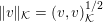 $\Vert v\Vert _{{\mathcal{K}}}=(v,v)_{{\mathcal{K}}}^{1/2}$
. For
 $v,w\in H^{1}({\mathcal{K}})$
and
 $\unicode[STIX]{x1D705},\unicode[STIX]{x1D705}^{\prime }\in {\mathcal{K}}$
, define the average and jump operators on a face
 $\overline{\unicode[STIX]{x1D705}}\cap \overline{\unicode[STIX]{x1D705}}^{\prime }$
by
 $$\begin{eqnarray}\langle v\rangle =\displaystyle \frac{1}{2}(v|_{\unicode[STIX]{x1D705}}+v|_{\unicode[STIX]{x1D705}^{\prime }}),\quad \langle \unicode[STIX]{x1D6FB}v\rangle =\displaystyle \frac{1}{2}(\unicode[STIX]{x1D6FB}v|_{\unicode[STIX]{x1D705}}+\unicode[STIX]{x1D6FB}v|_{\unicode[STIX]{x1D705}^{\prime }}),\end{eqnarray}$$
and
 $$\begin{eqnarray}\big[\hspace{-1.99168pt}\big[v\big]\hspace{-1.99168pt}\big]=v|_{\unicode[STIX]{x1D705}}\mathbf{n}_{\unicode[STIX]{x1D705}}+v|_{\unicode[STIX]{x1D705}^{\prime }}\mathbf{n}_{\unicode[STIX]{x1D705}^{\prime }},\quad \big[\hspace{-1.99168pt}\big[\unicode[STIX]{x1D6FB}v\big]\hspace{-1.99168pt}\big]=\unicode[STIX]{x1D6FB}v|_{\unicode[STIX]{x1D705}}\cdot \mathbf{n}_{\unicode[STIX]{x1D705}}+\unicode[STIX]{x1D6FB}v|_{\unicode[STIX]{x1D705}^{\prime }}\cdot \mathbf{n}_{\unicode[STIX]{x1D705}^{\prime }},\end{eqnarray}$$
where
 $\mathbf{n}_{\unicode[STIX]{x1D705}}$
denotes the exterior unit normal of the element
 $\unicode[STIX]{x1D705}$
.
In order to solve Kohn–Sham DFT in the broken Sobolev space
 $H^{1}({\mathcal{K}})$
, we also need to identify a basis set which spans a subspace of
 $H^{1}({\mathcal{K}})$
. Let
 $N_{\unicode[STIX]{x1D705}}$
be the number of DOFs on
 $\unicode[STIX]{x1D705}$
, and the total number of DOFs is
 $N_{b}=\sum _{\unicode[STIX]{x1D705}\in {\mathcal{K}}}N_{\unicode[STIX]{x1D705}}$
. Let
 $\mathbb{V}(\unicode[STIX]{x1D705})=\text{span}\{\unicode[STIX]{x1D719}_{\unicode[STIX]{x1D705},j}\}_{j=1}^{N_{\unicode[STIX]{x1D705}}}$
, where each
 $\unicode[STIX]{x1D719}_{\unicode[STIX]{x1D705},j}$
is a function defined on
 $\unicode[STIX]{x1D6FA}$
compactly supported in
 $\unicode[STIX]{x1D705}$
. Hence
 $\mathbb{V}(\unicode[STIX]{x1D705})$
is a subspace of
 $H^{1}({\mathcal{K}})$
and is associated with a finite-dimensional approximation for
 $H^{1}(\unicode[STIX]{x1D705})$
. Then
 $\mathbb{V}=\bigoplus _{\unicode[STIX]{x1D705}\in {\mathcal{K}}}\mathbb{V}(\unicode[STIX]{x1D705})$
is a finite-dimensional approximation to
 $H^{1}({\mathcal{K}})$
. We also assume all functions
 $\{\unicode[STIX]{x1D719}_{\unicode[STIX]{x1D705},j}\}$
form an orthonormal set in the sense that
 $$\begin{eqnarray}(\unicode[STIX]{x1D719}_{\unicode[STIX]{x1D705},j},\unicode[STIX]{x1D719}_{\unicode[STIX]{x1D705}^{\prime },j^{\prime }})_{{\mathcal{K}}}=\unicode[STIX]{x1D6FF}_{\unicode[STIX]{x1D705},\unicode[STIX]{x1D705}^{\prime }}\unicode[STIX]{x1D6FF}_{j,j^{\prime }},\quad \text{for all}~\unicode[STIX]{x1D705},\unicode[STIX]{x1D705}^{\prime }\in {\mathcal{K}},1\leq j\leq N_{\unicode[STIX]{x1D705}},1\leq j^{\prime }\leq N_{\unicode[STIX]{x1D705}^{\prime }}.\end{eqnarray}$$
For the moment, we assume that the basis set
 $\mathbb{V}$
has been given. For
 $w,v\in \mathbb{V}$
, we introduce the following bilinear form:
 $$\begin{eqnarray}\displaystyle a(w,v) & = & \displaystyle \mathop{\sum }_{\unicode[STIX]{x1D705}\in {\mathcal{K}}}\bigg[\displaystyle \frac{1}{2}(\unicode[STIX]{x1D6FB}w,\unicode[STIX]{x1D6FB}v)_{\unicode[STIX]{x1D705}}+((V_{\text{eff}}+V_{\text{nl}})w,v)_{\unicode[STIX]{x1D705}}\nonumber\\ \displaystyle & & \displaystyle \qquad -(\unicode[STIX]{x1D6FB}w,\big[\hspace{-1.99168pt}\big[\unicode[STIX]{x1D713}_{v}\big]\hspace{-1.99168pt}\big])_{\unicode[STIX]{x2202}\unicode[STIX]{x1D705}}-(\big[\hspace{-1.99168pt}\big[w\big]\hspace{-1.99168pt}\big],\unicode[STIX]{x1D6FB}v)_{\unicode[STIX]{x2202}\unicode[STIX]{x1D705}}+\unicode[STIX]{x1D6FC}(\big[\hspace{-1.99168pt}\big[w\big]\hspace{-1.99168pt}\big],\big[\hspace{-1.99168pt}\big[v\big]\hspace{-1.99168pt}\big])_{\unicode[STIX]{x2202}\unicode[STIX]{x1D705}}\bigg].\end{eqnarray}$$
Here the first term on the right-hand side is the kinetic energy, and the second term is the effective local potential and the non-local potential as in equation (2.91). The third and fourth terms are obtained from integration by parts of the Laplacian operator, which cures the ill-defined operation of applying the Laplacian operator to discontinuous functions on the global domain. The last term is a penalty term to guarantee the stability condition (Arnold, Brezzi, Cockburn and Marini Reference Arnold, Brezzi, Cockburn and Marini2002). The penalty parameter needs to be sufficiently large, and the value of
 $\unicode[STIX]{x1D6FC}$
depends on the choice of basis set
 $\mathbb{V}$
.
In order to find the approximate Kohn–Sham orbitals
 $\{\unicode[STIX]{x1D713}_{i}\}_{i=1}^{N}\subset \mathbb{V}$
, that is,
 $$\begin{eqnarray}\unicode[STIX]{x1D713}_{i}(\mathbf{r})=\mathop{\sum }_{\unicode[STIX]{x1D705}}\mathop{\sum }_{j=1}^{N_{\unicode[STIX]{x1D705}}}c_{\unicode[STIX]{x1D705},j;i}\unicode[STIX]{x1D719}_{\unicode[STIX]{x1D705},j}(\mathbf{r}),\end{eqnarray}$$
we minimize the following energy functional:
 $$\begin{eqnarray}{\mathcal{E}}^{\text{DG}}(\{\unicode[STIX]{x1D713}_{i}\})=\mathop{\sum }_{i=1}^{N}a(\unicode[STIX]{x1D713}_{i},\unicode[STIX]{x1D713}_{i}),\end{eqnarray}$$
subject to the orthonormal constraint for
 $\{\unicode[STIX]{x1D713}_{i}\}$
. The associated Euler–Lagrange equation corresponding to this minimization problem gives rise to the following eigenvalue problem:
 $$\begin{eqnarray}\mathop{\sum }_{\unicode[STIX]{x1D705}^{\prime },j^{\prime }}H_{\unicode[STIX]{x1D705},j;\unicode[STIX]{x1D705}^{\prime },j^{\prime }}^{\text{DG}}c_{\unicode[STIX]{x1D705}^{\prime },j^{\prime };i}=\unicode[STIX]{x1D700}_{i}^{\text{DG}}c_{\unicode[STIX]{x1D705},j;i},\quad i=1,\ldots ,N,\end{eqnarray}$$
where the projected Hamiltonian matrix is given by
 $$\begin{eqnarray}H_{\unicode[STIX]{x1D705},j;\unicode[STIX]{x1D705}^{\prime },j^{\prime }}^{\text{DG}}=a(\unicode[STIX]{x1D719}_{\unicode[STIX]{x1D705},j},\unicode[STIX]{x1D719}_{\unicode[STIX]{x1D705}^{\prime },j^{\prime }}).\end{eqnarray}$$
(Credit: Hu, Lin and Yang Reference Hu, Lin and Yang2015.) A model system in 2D partitioned into
 $16$
(4
 $\times$
4) equal-sized elements. The elements are denoted by
 $E_{i}$
.
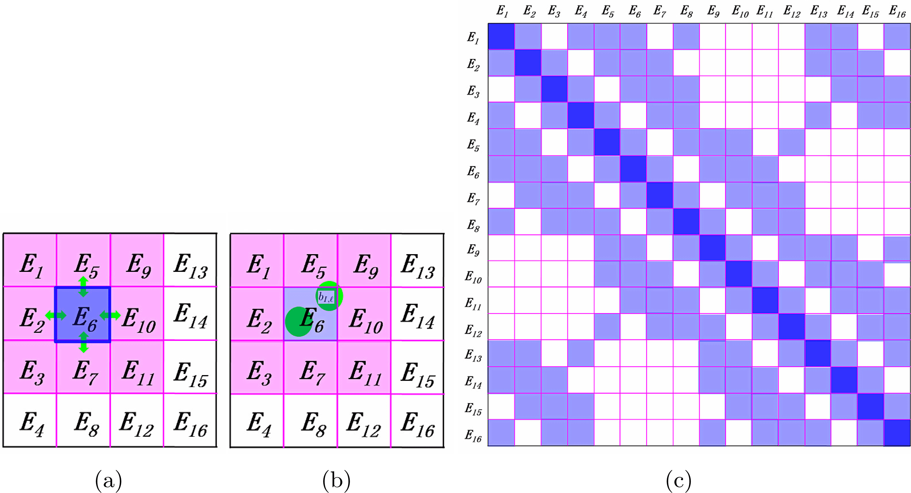
The
 $H^{\text{DG}}$
matrix can be naturally partitioned into matrix blocks as sketched in Figure 3.2. The kinetic energy and the local pseudopotential can only contribute to the diagonal matrix blocks. The terms from boundary integrals can contribute to both the diagonal and the off-diagonal blocks of
 $H^{\text{DG}}$
corresponding to adjacent elements. Each boundary term involves only two neighbouring elements by definition, as plotted in Figure 3.2(a). For the non-local pseudopotential, since a projection vector of the non-local pseudopotential is spatially localized, we require the dimension of every element along each direction (usually around
 $6\sim 8$
Bohr) to be larger than the size of the non-zero support of each projection vector (usually around
 $2\sim 4$
Bohr). Thus, the non-zero support of each projection vector can overlap with at most
 $2^{d}$
elements as shown in Figure 3.2(b) (
 $d=1,2,3$
). As a result, each non-local pseudopotential term may also contribute to both the diagonal and the off-diagonal blocks corresponding to adjacent elements. In summary,
 $H^{\text{DG}}$
is a sparse matrix and the non-zero matrix blocks correspond to interactions between neighbouring elements (Figure 3.2(c)).
From the solution of the eigenvalue problem (3.29), we may compute the electron density as
 $$\begin{eqnarray}\unicode[STIX]{x1D70C}(\mathbf{r})=\mathop{\sum }_{i=1}^{N}\mathop{\sum }_{\unicode[STIX]{x1D705}}\bigg|\mathop{\sum }_{j}c_{\unicode[STIX]{x1D705},j;i}\unicode[STIX]{x1D719}_{\unicode[STIX]{x1D705},j}(\mathbf{r})\bigg|^{2}.\end{eqnarray}$$
Note that the computation of the electron density can be performed locally in each element due to the locality of the basis functions
 $\unicode[STIX]{x1D719}_{\unicode[STIX]{x1D705},j}$
. Then the electron density can be fed back to the next step of the SCF iteration.
There are several methods to generate the basis set
 $\mathbb{V}$
in the broken Sobolev space. Here we introduce the adaptive local basis set in Lin et al. (Reference Lin, Lu, Ying and E2012a
), which is obtained by solving local Kohn–Sham problems. For each element
 $\unicode[STIX]{x1D705}$
, we form an extended element
 $\widetilde{\unicode[STIX]{x1D705}}$
around
 $\unicode[STIX]{x1D705}$
, and we refer to
 $\widetilde{\unicode[STIX]{x1D705}}\backslash \unicode[STIX]{x1D705}$
as the buffer region for
 $\unicode[STIX]{x1D705}$
. On
 $\widetilde{\unicode[STIX]{x1D705}}$
we solve the eigenvalue problem
 $$\begin{eqnarray}\biggl(-\displaystyle \frac{1}{2}\unicode[STIX]{x1D6E5}+V_{\text{eff}}^{\widetilde{\unicode[STIX]{x1D705}}}+V_{\text{nl}}^{\widetilde{\unicode[STIX]{x1D705}}}\biggr)\widetilde{\unicode[STIX]{x1D719}}_{\unicode[STIX]{x1D705},j}=\unicode[STIX]{x1D706}_{\unicode[STIX]{x1D705},j}\widetilde{\unicode[STIX]{x1D719}}_{\unicode[STIX]{x1D705},j}.\end{eqnarray}$$
with certain boundary conditions on
 $\unicode[STIX]{x2202}\widetilde{\unicode[STIX]{x1D705}}$
. Here we define
 $V_{\text{eff}}^{\widetilde{\unicode[STIX]{x1D705}}}=V_{\text{eff}}|_{\widetilde{\unicode[STIX]{x1D705}}}$
to be the restriction of the effective potential at the current SCF step to
 $\widetilde{\unicode[STIX]{x1D705}}$
, and
 $V_{\text{nl}}^{\widetilde{\unicode[STIX]{x1D705}}}=V_{\text{nl}}|_{\widetilde{\unicode[STIX]{x1D705}}}$
to be the restriction of the non-local potential to
 $\widetilde{\unicode[STIX]{x1D705}}$
. This eigenvalue problem can be solved using a standard basis set such as finite difference, finite elements or planewaves. Note that the size of the extended element
 $\widetilde{\unicode[STIX]{x1D705}}$
is independent of the size of the global domain, and so is the number of basis functions per element. We then restrict
 $\{\widetilde{\unicode[STIX]{x1D719}}_{\unicode[STIX]{x1D705},j}\}$
from
 $\widetilde{\unicode[STIX]{x1D705}}$
to
 $\unicode[STIX]{x1D705}$
. The truncated functions are not necessarily orthonormal. Therefore, we apply a singular value decomposition (SVD) to obtain
 $\{\unicode[STIX]{x1D719}_{\unicode[STIX]{x1D705},j}\}$
. The SVD procedure can ensure the orthonormal constraint of the basis functions inside each element, as well as eliminating the approximately linearly dependent functions in the basis set. We then extend each
 $\unicode[STIX]{x1D719}_{k,j}$
to the global domain by setting it to zero outside
 $\unicode[STIX]{x1D705}$
to generate the basis set
 $\mathbb{V}$
. As a result, the overlap matrix corresponding to the adaptive local basis set is an identity matrix.
There are a number of possible ways to set the boundary conditions for the local problem (3.32). In practice, we use the periodic boundary condition for all eigenfunctions
 $\{\widetilde{\unicode[STIX]{x1D719}}_{\unicode[STIX]{x1D705},j}\}$
in
 $\widetilde{\unicode[STIX]{x1D705}}$
. In some sense, the details of the boundary condition do not affect the accuracy of the adaptive local basis set much as the buffer size increases. The periodic boundary condition permits the use of Fourier basis sets for solving the local problem. Note that while the eigenfunctions are required to satisfy periodic boundary conditions, the potential is obtained from the restriction of the global Kohn–Sham potential to the extended element. The size of each extended element should be chosen to balance between the effectiveness of the basis functions and the computational cost of obtaining them. For a typical choice used in practice, the elements are chosen to be of the same size, and each element contains on average a few atoms. The partition does not need to be updated when the atomic configuration is changed, as in the case of structure optimization and molecular dynamics.
Once the SCF iteration reaches convergence, we may evaluate the atomic forces. Recall the discussion in Section 2.8 that the atomic force generally consists of two components: the Hellmann–Feynman force and the Pulay force. Since each ALB depends on the atomic configuration, the Pulay force does not vanish as in the planewave basis set. Compared to atomic orbitals, the Pulay force for the adaptive basis set is much more difficult to evaluate. Nonetheless, the adaptive basis sets are constructed to be aware of the environment of each atom, and can be much closer to a complete basis set for describing occupied states than numerical atomic orbitals. Numerical results indicate that the Pulay force for the atomic basis set is indeed small, and use of the Hellman–Feynman formula can readily achieve chemical accuracy (Zhang et al.
Reference Zhang, Lin, Hu, Yang and Pask2017). We also remark that using the spatial locality of the basis set
 $\mathbb{V}$
, the computational cost of evaluating the force for all atoms can be reduced from
 $O(N^{2})$
to
 $O(N)$
. Compared to equation (2.95), the main reduction of the computational cost comes from (i) the localized pseudocharge associated with the local pseudopotential
 $V_{\text{loc},I}$
(the pseudocharge is defined as
 $-\unicode[STIX]{x1D6E5}V_{\text{loc},I}/4\unicode[STIX]{x1D70B}$
), and (ii) the density matrix formulation for the contribution from the non-local pseudopotential. We refer readers to Zhang et al. (Reference Zhang, Lin, Hu, Yang and Pask2017) for more details.
The adaptive local basis set and the DG formulation have been implemented in the DGDFT (discontinuous Galerkin density functional theory) software package. DGDFT is a massively parallel electronic structure software package designed for large-scale DFT calculations involving up to tens of thousands of atoms (Hu et al.
Reference Hu, Lin and Yang2015). As an illustrating example, Figure 3.3 shows the ALBs of a 2D phosphorene monolayer with
 $140$
phosphorus atoms (P
 $_{140}$
). This is a two-dimensional system, and the global domain is partitioned into
 $64$
equal-sized elements along the
 $Y$
and
 $Z$
directions, respectively. We show the isosurfaces of the first three ALB functions for the element denoted by
 $E_{10}$
in Figure 3.3(a–c). Each ALB function shown is strictly localized inside
 $E_{10}$
and is therefore discontinuous across the boundary of elements. On the other hand, each ALB function is delocalized across a few atoms inside the element since they are obtained from eigenfunctions of local Kohn–Sham Hamiltonian. Although the basis functions are discontinuous, the electron density is well-defined and is very close to being a continuous function in the global domain (Figure 3.3(d)).
(Credit: Hu et al.
Reference Hu, Lin and Yang2015.) The P
 $_{140}$
system, with the isosurfaces (0.04 Hartree/Bohr
 $^{3}$
) of the first three ALB functions belonging to the tenth element
 $E_{10}$
: (a)
 $\unicode[STIX]{x1D719}_{1}$
, (b)
 $\unicode[STIX]{x1D719}_{2}$
, (c)
 $\unicode[STIX]{x1D719}_{3}$
and (d) the electron density
 $\unicode[STIX]{x1D70C}$
in the top and side views in the global domain in the example of P
 $_{140}$
. The red and blue regions indicate positive and negative isosurfaces, respectively. There are 64 elements and 80 ALB functions in each element, corresponding to
 $37$
basis functions per atom.
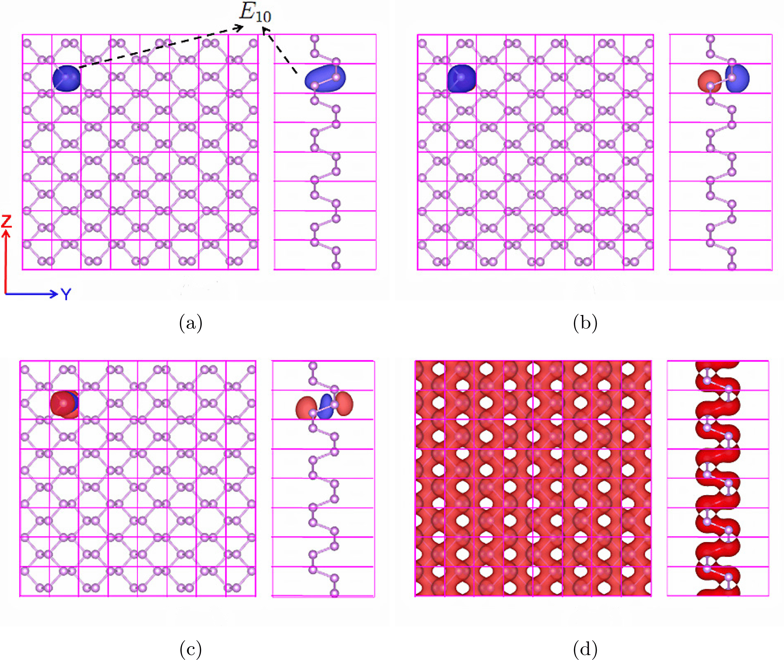
Figure 3.4 shows the convergence of the total energy and atomic forces for the quasi-1D and 3D Si systems with an increasing number of ALB functions per atom. First, we see that chemical accuracy is obtained with less than ten basis functions per atom for the quasi-1D system and a few tens of basis functions per atom for the 3D system. Furthermore, for the quasi-1D Si system, we find that the total energy error can be as small as 2.78
 $\times$
10
 $^{-8}$
Ha/atom and the maximum error of the atomic forces can be as small as 8.47
 $\times$
10
 $^{-7}$
Ha/Bohr when 22.5 ALB functions per atom are used. For the bulk 3D Si system, the total energy error can be as small as 2.10
 $\times$
10
 $^{-6}$
Ha/atom and the maximum error in atomic forces can be as small as 1.70
 $\times$
10
 $^{-5}$
Ha/Bohr when 71.11 ALB functions per atom are used.
(Credit: Zhang et al.
Reference Zhang, Lin, Hu, Yang and Pask2017.) Convergence of DGDFT total energy and forces for quasi-1D and 3D Si systems to reference planewave results with increasing number of ALB functions per atom. (a) Total energy error per atom
 $\unicode[STIX]{x1D6E5}E$
(Ha/atom). (b) Maximum atomic force error
 $\unicode[STIX]{x1D6E5}F$
(Ha/Bohr). The dashed green line corresponds to chemical accuracy. We set
 $E_{\text{cut}}=60$
Ha and penalty parameter
 $\unicode[STIX]{x1D6FC}=40$
. When the number of basis functions per atom is sufficiently large, the error is well below the target accuracy (green dashed line).
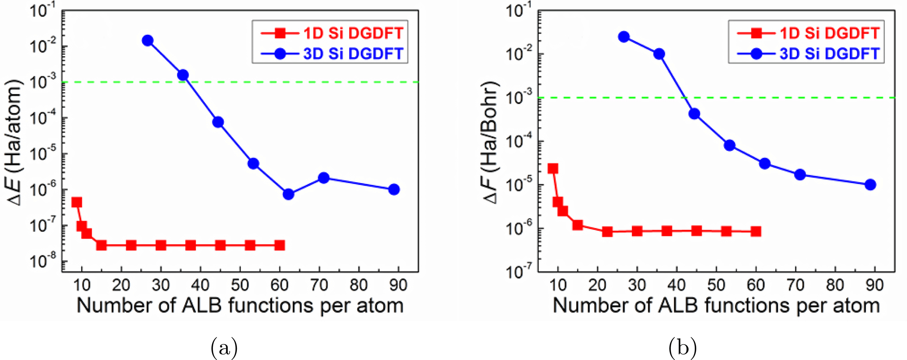
Remarks
The adaptive basis set is closely related to the ‘hybrid basis set’, which directly combines the large basis set and the small basis set. The idea of such a combination dates back to Slater in his augmented planewave method (APW) (Slater Reference Slater1937), which was later improved to become the linearized APW method (Andersen Reference Andersen1975). The idea is to use an atomic basis set near the atom to resolve the singularity due to the electron–nucleus interaction in all-electron calculations, and use smooth functions such as planewaves in the interstitial region. Since planewaves are used without compression, the number of degrees of freedom per atom in the hybrid basis set is still relatively large. Recently there have been further developments along this direction using a partition of unity approach (Cai, Bai, Pask and Sukumar Reference Cai, Bai, Pask and Sukumar2013) and the discontinuous Galerkin approach (Lu, Cai, Xin and Guo Reference Lu, Cai, Xin and Guo2013).
The interior penalty formulation of DG requires setting a penalty parameter. For general non-polynomial basis functions, the value of the penalty parameter is not known a priori. We have demonstrated that the adjustable penalty parameter is mainly used to ensure the stability of the numerical scheme, and has relatively little effect on the accuracy of the scheme when it takes a large range of values (Lin et al.
Reference Lin, Lu, Ying and E2012a
, Hu et al.
Reference Hu, Lin and Yang2015). Another possible solution can be found in Lin and Stamm (Reference Lin and Stamm2016), which provides a formula for evaluating
 $\unicode[STIX]{x1D6FC}$
on the fly for general non-polynomial basis sets based on the solution of eigenvalue problems restricted to each element
 $\unicode[STIX]{x1D705}$
. This further leads to rigorous a posteriori error estimates for using non-polynomial basis functions in the DG setting to solve linear PDEs and eigenvalue problems (Kaye, Lin and Yang Reference Kaye, Lin and Yang2015, Lin and Stamm Reference Lin and Stamm2016, Reference Lin and Stamm2017). This allows adaptive refinement of the basis set to improve its efficiency for heterogeneous systems.
The adaptive local basis set has been improved in a number of directions. As in the NGWF approach, the adaptive local basis set can be obtained via numerical optimization (Lin, Lu, Ying and E Reference Lin, Lu, Ying and E2012b ), which rigorously eliminates the Pulay force when the minimizer is achieved. The basis functions can also be obtained from solutions to linear systems on the global domain, which removes the need to impose artificial boundary conditions on the extended element and simultaneously improves the accuracy of the basis set (Li and Lin Reference Li and Lin2019). The adaptive local basis set can also be constructed by partitioning the discretized basis indices instead of the continuous domain (Xu, Suryanarayana and Pask Reference Xu, Suryanarayana and Pask2018). This is called the discrete discontinuous basis projection method. Formally, this is a Galerkin method instead of a discontinuous Galerkin approach, and the advantage of this method is that it removes the need to impose penalty conditions on the basis set.
4 Algorithmic tools
This section introduces a few algorithmic tools that are useful in electronic structure calculations. We introduce direct and iterative eigensolvers in Sections 4.1 and 4.2, respectively. These are the standard methods for solving the eigenvalue problem obtained in Kohn–Sham DFT after discretization. In Section 4.3 we discuss how to compress information on the Kohn–Sham orbitals through localization. Localized representation of the occupied space forms the basis for linear scaling algorithms for insulating systems to be discussed in Section 5.2. Then in Section 4.4 we introduce the interpolative separable density fitting (ISDF) technique to compress the information stored in the pair products of Kohn–Sham orbitals, which will become useful in reducing the computational cost of Kohn–Sham DFT calculations with rung-4 and rung-5 functionals. We remark that eigensolvers, localization and density fitting are generic techniques that are useful in a number of other contexts of scientific computing. Hence we summarize these techniques separately in this section.
4.1 Direct diagonalization methods
When a small basis set is used and the system size is not too large, it is most efficient to solve the standard or generalized eigenvalue problem (3.14) using a generic eigensolver for dense matrices. It can be performed in serial using the LAPACK software package (Anderson et al.
Reference Anderson, Bai, Bischof, Blackford, Demmel, Dongarra, Du Croz, Greenbaum, Hammarling, McKenney and Sorensen1999) or in parallel using the ScaLAPACK software package (Blackford et al.
Reference Blackford, Choi, Cleary, D’Azevedo, Demmel, Dhillon, Hammarling, Henry, Petitet, Stanley, Walker and Whaley1997). Recently dense solvers specialized for solving large-scale Hermitian eigenvalue problems, such as ELPA (Marek et al.
Reference Marek, Blum, Johanni, Havu, Lang, Auckenthaler, Heinecke, Bungartz and Lederer2014), have been demonstrated to be more efficient and to scale massively in parallel to more than
 $100\,000$
computational cores. As a rule of thumb, dense eigensolvers are most efficient when the matrix dimension is
 $10\,000$
or less, but are not commonly used when the matrix dimension is beyond
 $100\,000$
, due to the steep increase of the computational cost that scales as
 $O(N_{b}^{3})$
.
4.2 Iterative diagonalization methods
When a large basis set is used, iterative diagonalization methods that rely on the matrix–vector product of
 $H^{\text{KS}}[\unicode[STIX]{x1D70C}]$
with arbitrary vectors become particularly attractive, especially when the matrix–vector product can be performed efficiently. The two common cases are when
 $H^{\text{KS}}[\unicode[STIX]{x1D70C}]$
is sparse and when
 $H^{\text{KS}}[\unicode[STIX]{x1D70C}]$
is constructed using the Fourier basis set so that the fast Fourier transform can be used. Among the iterative diagonalization methods, we focus on Krylov subspace methods here. The discussion of another class of methods called filtering methods will be deferred to Section 5.1.
The key idea of Krylov subspace methods is to form a low-dimensional subspace and approximate the eigenpairs with those of the projected Hamiltonian into this subspace. Of these methods, the Davidson–Liu method (Davidson Reference Davidson1975, Liu Reference Liu1978) and the LOBPCG method (Knyazev Reference Knyazev2001) are widely used due to their simplicity and efficiency.
Consider for simplicity the standard eigenvalue problem
 $$\begin{eqnarray}HX=X\unicode[STIX]{x1D6EC},\end{eqnarray}$$
where the columns of the
 $N_{b}\times N$
matrix
 $X$
are the eigenvectors and the diagonal entries of the
 $N\times N$
diagonal matrix
 $\unicode[STIX]{x1D6EC}$
give the eigenvalues.
In its simplest version, the Davidson–Liu method solves this problem by iteratively minimizing
 $\text{Tr}[X^{\ast }HX]$
over a matrix
 $X$
that satisfies the orthogonality constraint
 $X^{\ast }X=I$
and takes its columns from a subspace spanned by a collection of
 $2N$
vectors. These
 $2N$
vectors are set to be the columns of the matrix
 $X$
from the previous step and another
 $N_{b}\times N$
matrix
 $W$
, which is a preconditioned residual of
 $X$
. More precisely, in each iteration one updates
 $X$
via
 $$\begin{eqnarray}X\leftarrow XC_{X}+WC_{W},\quad W=TR:=T(HX-X(X^{\ast }HX)),\end{eqnarray}$$
where
 $R=HX-X(X^{\ast }HX)$
is the residual and
 $T$
is a preconditioner that is ideally close to
 $(H-\unicode[STIX]{x1D706}I)^{-1}$
with a certain shift
 $\unicode[STIX]{x1D706}$
. The original version of the Davidson–Liu method allows one to use many copies of the history; here, in order to simplify the discussion, we keep only the most recent copy of
 $X$
and
 $W$
. The coefficients
 $C_{X}$
and
 $C_{W}$
are obtained by computing the lowest
 $N$
eigenpairs of the projected
 $2N$
 $\times$
 $2N$
generalized eigenvalue problem
 $$\begin{eqnarray}S^{\ast }HSC=S^{\ast }SC\unicode[STIX]{x1D6EC},\quad C=\left[\begin{array}{@{}c@{}}C_{X}\\ C_{W}\end{array}\right]\in \mathbb{R}^{2N\times N},\end{eqnarray}$$
where
 $S=[X,W]\in \mathbb{R}^{N_{b}\times 2N}$
represents the trial subspace and
 $C$
contains the optimal coefficients. The Davidson–Liu method is summarized in Algorithm 1.

The LOBPCG algorithm improves on the Davidson–Liu algorithm by introducing a conjugate search direction. More precisely, it solves
 $HX=X\unicode[STIX]{x1D6EC}$
by iteratively minimizing
 $\text{Tr}[X^{\ast }HX]$
over
 $X$
that satisfies the orthogonality constraint
 $X^{\ast }X=I$
and takes its columns from a subspace spanned by
 $3N$
vectors. These
 $3N$
vectors are the columns of the matrix
 $X$
of the previous step, its preconditioned residual
 $W$
and an extra matrix
 $P$
that consists of certain conjugate directions. The coefficients
 $C_{X}$
,
 $C_{W}$
and
 $C_{P}$
are obtained by computing the lowest
 $N$
eigenpairs of the projected
 $3N$
 $\times$
 $3N$
generalized eigenvalue problem
 $$\begin{eqnarray}S^{\ast }HSC=S^{\ast }SC\unicode[STIX]{x1D6EC},\quad C=\left[\begin{array}{@{}c@{}}C_{X}\\ C_{W}\\ C_{P}\end{array}\right]\in \mathbb{R}^{3N\times N},\end{eqnarray}$$
where
 $S=[X,W,P]$
is the trial subspace. The LOBPCG method is outlined in Algorithm 2.

Note that when
 $N$
is relatively small (
 $N\sim 10$
–
 $1000$
), the computational cost of the
 $2N\times 2N$
or
 $3N\times 3N$
projected eigenvalue problem in the Rayleigh–Ritz step is negligible. However, when
 $N$
is relatively large (
 $N\sim 1000$
–
 $10\,000$
), the cost of solving such projected eigenvalue problems can become dominant. Furthermore, even with recent advances in dense eigensolvers such as ELPA (Marek et al.
Reference Marek, Blum, Johanni, Havu, Lang, Auckenthaler, Heinecke, Bungartz and Lederer2014), the Rayleigh–Ritz step can still limit the parallel scalability and dominate the wall clock time of the Davidson–Liu and LOBPCG algorithms when a large number of processors are used.
More recently, the projected preconditioned conjugate gradient (PPCG) (Vecharynski, Yang and Pask Reference Vecharynski, Yang and Pask2015) algorithm has been proposed to reduce the cost of the Rayleigh–Ritz step. The main idea of PPCG is to replace the
 $3N\times 3N$
projected eigenvalue problem of LOBPCG by
 $N$
subproblems, each of size
 $3\times 3$
. Compared to the solution of the subspace problem from a full Rayleigh–Ritz step, PPCG relaxes the optimality of the search direction at each step, but the advantage is that all
 $N$
subproblems can be solved independently. The computational cost of this step scales linearly with
 $N$
, and is negligibly small even when
 $N$
is large. The orbitals still need to be orthogonalized at each step to avoid degeneracy. We remark that the idea of the PPCG method is closely related to another variant of the LOBPCG method called LOBPCG II (Knyazev Reference Knyazev2001).
Remarks
Algorithms 1 and 2 update all columns of
 $X$
simultaneously. This is often referred to as a block eigensolver, which can efficiently utilize BLAS 3 level matrix–matrix multiplication operations, and is suitable for parallelization. The disadvantage of a block eigensolver is that the cost of the Rayleigh–Ritz step can be expensive when
 $N$
becomes large. Different eigenvectors often converge with different rates, and the subspace problem may thus become degenerate. In such a case, the converged eigenvectors should be deflated from the unconverged ones to avoid instability. Another strategy is to solve the eigenpairs one by one, starting from the smallest eigenvalue. Such a method is often referred to as a single-band method (Payne et al.
Reference Payne, Teter, Allen, Arias and Joannopoulos1992) in electronic structure calculation. Since each eigenvector is directly orthogonalized with all previously converged eigenvectors, the single-band method can be numerically more stable. Besides the eigensolvers mentioned in this section, the linear eigenvalue problem can also be solved via optimization methods under orthogonality constraints (Payne et al.
Reference Payne, Teter, Allen, Arias and Joannopoulos1992, Edelman, Arias and Smith Reference Edelman, Arias and Smith1998, Yang, Meza and Wang Reference Yang, Meza and Wang2006, Wen and Yin Reference Wen and Yin2013). We also remark that optimization techniques can be used to minimize the nonlinear Kohn–Sham energy functional directly with respect to the Kohn–Sham orbitals.
The choice of the preconditioner
 $T$
can significantly affect the convergence rate of eigensolvers. In the context of the planewave basis set, the most commonly used preconditioner (Teter, Payne and Allan Reference Teter, Payne and Allan1989) is diagonal in frequency space,
 $T=F^{-1}\hat{T}F$
, where
 $F$
is the discrete Fourier transform matrix, with the coefficients
 $\hat{T}$
given by
 $$\begin{eqnarray}\hat{T}(\mathbf{g},\mathbf{g}^{\prime })=\unicode[STIX]{x1D6FF}_{\boldsymbol{ g},\mathbf{g}^{\prime }}\biggl(\displaystyle \frac{27+18E_{\mathbf{g}}+12E_{\mathbf{g}}^{2}+8E_{\mathbf{g}}^{3}}{27+18E_{\mathbf{g}}+12E_{\mathbf{g}}^{2}+8E_{\mathbf{g}}^{3}+16E_{\mathbf{g}}^{4}}\biggr),\end{eqnarray}$$
where
 $E_{\mathbf{g}}=|\mathbf{g}|^{2}/2$
is the kinetic energy associated with the Fourier mode
 $\mathbf{g}$
. The purpose of the choice (4.1) is that the Fourier modes of long wavelengths (i.e.
 $|\mathbf{g}|$
is small) remain approximately unchanged, while Fourier modes of short wavelengths (i.e.
 $|\mathbf{g}|$
is large) are dampened by
 $1/E_{\mathbf{g}}$
, which is approximately
 $2(-\unicode[STIX]{x1D6E5})^{-1}$
. The rationale is that the Laplacian operator is an unbounded operator, while the pseudopotential, Hartree and exchange-correlation potentials are usually bounded operators. As the planewave basis set is being refined, the Laplacian operator dominates the spectral radius of the Hamiltonian, especially along the Fourier modes with short wavelengths. Hence, along such modes, the preconditioner
 $T$
approximates
 $H^{-1}$
well.
The preconditioner (4.1) can be efficiently implemented in the context of the planewave basis set using only two FFTs per orbital, but it becomes considerably more difficult in other large basis sets such as the finite element method, and the finite difference method. In such a case, one often performs preconditioning by directly taking
 $T=-\unicode[STIX]{x1D6E5}^{-1}$
, and applying the preconditioner to the residual vector
 $r$
amounts to solving a Poisson equation.
4.3 Localization methods
Localized representations of electronic wavefunctions have a wide range of applications in quantum physics, chemistry and materials science. As they require significantly less cost for both storage and computation, localized representations are the foundation of so-called ‘linear scaling methods’ (Kohn Reference Kohn1996, Goedecker Reference Goedecker1999, Bowler and Miyazaki Reference Bowler and Miyazaki2012) for solving quantum problems (see more discussion in Section 5.2). They can also be used to analyse the chemical bonding in complex materials, interpolate the band structure of crystals, accelerate ground and excited state electronic structure calculations, and form reduced-order models for strongly correlated many-body systems (Marzari et al. Reference Marzari, Mostofi, Yates, Souza and Vanderbilt2012).
The localization problem can be stated as follows. The Kohn–Sham orbitals
 $\{\unicode[STIX]{x1D713}_{i}\}_{i=1}^{N}$
are eigenfunctions of a Hamiltonian matrix, and are generally delocalized across the entire system, i.e. with significant magnitude in large portions of the computational domain. Nonetheless, if we apply a unitary rotation
 $U\in \mathbb{C}^{N\times N}$
to the Kohn–Sham orbitals
 $$\begin{eqnarray}w_{i}(\mathbf{r})=\mathop{\sum }_{j=1}^{N}\unicode[STIX]{x1D713}_{j}(\mathbf{r})U_{ji},\end{eqnarray}$$
the density matrix and hence the electron density are invariant with respect to such rotation. However, for certain systems there exist unitary transformations for which the resulting orthonormal functions
 $\{w_{i}\}_{i=1}^{N}$
are approximately only supported on a small portion of the computational domain. For isolated systems,
 $\{w_{i}\}_{i=1}^{N}$
are often called Boys orbitals (Foster and Boys Reference Foster and Boys1960), while for periodic systems they are often called Wannier functions (Wannier Reference Wannier1937). Below we will simply refer to the localized orbitals as Wannier functions.
For isolated systems surrounded by a vacuum, the occupied orbitals always decay exponentially to zero as
 $|\mathbf{r}|\rightarrow \infty$
(Lieb and Loss Reference Lieb and Loss2001). Hence qualitatively, both the Kohn–Sham orbitals
 $\unicode[STIX]{x1D713}_{i}$
and the localized orbitals
 $w_{i}$
decay exponentially, and the localization is defined only in a quantitative sense.
On the other hand, for periodic crystals, the Kohn–Sham orbitals satisfy the Bloch boundary condition on each unit cell, and hence are delocalized on a macroscopic scale. However, for insulating systems with a finite band gap, the kernel of the density matrix decays exponentially along the off-diagonal direction (Kohn Reference Kohn1959, Blount Reference Blount1962, Nenciu Reference Nenciu1983, E and Lu Reference E and Lu2011, Benzi, Boito and Razouk Reference Benzi, Boito and Razouk2013, Lin and Lu Reference Lin and Lu2016), in the sense that
 $$\begin{eqnarray}|P(\mathbf{r},\mathbf{r}^{\prime })|\lesssim \text{e}^{-C|\mathbf{r}-\mathbf{r}^{\prime }|},\quad |\mathbf{r}-\mathbf{r}^{\prime }|\rightarrow \infty .\end{eqnarray}$$
This is related to the near-sightedness principle in the physics literature (Kohn Reference Kohn1996, Prodan and Kohn Reference Prodan and Kohn2005).
If the system is also topologically trivial, then one may further find a proper choice of the gauge to construct a set of exponentially localized Wannier functions (Kohn Reference Kohn1959, Blount Reference Blount1962, Kivelson Reference Kivelson1982, Nenciu Reference Nenciu1983, Brouder et al. Reference Brouder, Panati, Calandra, Mourougane and Marzari2007, Li and Lu Reference Li and Lu2010, Panati and Pisante Reference Panati and Pisante2013). Therefore, localized representation can make a qualitative difference. In the past few decades, many numerical algorithms have been designed to compute such localized orbitals (Marzari and Vanderbilt Reference Marzari and Vanderbilt1997, Koch and Goedecker Reference Koch and Goedecker2001, Gygi Reference Gygi2009, Damle, Lin and Ying Reference Damle, Lin and Ying2015, Mustafa, Coh, Cohen and Louie Reference Mustafa, Coh, Cohen and Louie2015, Cancès, Levitt, Panati and Stoltz Reference Cancès, Levitt, Panati and Stoltz2017, Damle, Lin and Ying Reference Damle, Lin and Ying2017, Damle and Lin Reference Damle and Lin2018).
For isolated systems, the localized representation can be identified by minimizing the following spread functional (Foster and Boys Reference Foster and Boys1960, Marzari and Vanderbilt Reference Marzari and Vanderbilt1997):
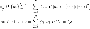 $$\begin{eqnarray}\displaystyle & & \displaystyle \inf _{U}\unicode[STIX]{x1D6FA}[\{w_{i}\}_{i=1}^{N}]=\mathop{\sum }_{i=1}^{N}[\langle w_{i}|\mathbf{r}^{2}|w_{i}\rangle -(\langle w_{i}|\mathbf{r}|w_{i}\rangle )^{2}]\nonumber\\ \displaystyle & & \displaystyle \;\text{subject to}~w_{i}=\mathop{\sum }_{j=1}^{N}\unicode[STIX]{x1D713}_{j}U_{ji},U^{\ast }U=I_{N}.\end{eqnarray}$$
In three-dimensional space, the formula for the functional
 $\unicode[STIX]{x1D6FA}$
should be interpreted as
 $$\begin{eqnarray}\mathop{\sum }_{\unicode[STIX]{x1D6FC}=1}^{3}[\langle w_{i}|\mathbf{r}_{\unicode[STIX]{x1D6FC}}^{2}|w_{i}\rangle -(\langle w_{i}|\mathbf{r}_{\unicode[STIX]{x1D6FC}}|w_{i}\rangle )^{2}]:=\langle w_{i}|(\mathbf{r}-\langle \mathbf{r}\rangle _{i})\cdot (\mathbf{r}-\langle \mathbf{r}\rangle _{i})|w_{i}\rangle ,\end{eqnarray}$$
where
 $\langle \mathbf{r}\rangle _{i}:=\langle w_{i}|\mathbf{r}|w_{i}\rangle$
. Hence the spread functional can be written compactly as
 $$\begin{eqnarray}\unicode[STIX]{x1D6FA}[\{w_{i}\}_{i=1}^{N}]=\mathop{\sum }_{i=1}^{N}\langle w_{i}|(\mathbf{r}-\langle \mathbf{r}\rangle _{i})^{2}|w_{i}\rangle .\end{eqnarray}$$
The functional
 $\unicode[STIX]{x1D6FA}$
characterizes the total spatial spread of the rotated orbitals
 $\{w_{i}\}$
, in terms of the second moment around each centre
 $\langle \mathbf{r}\rangle _{i}$
. A smaller spread value indicates a more localized representation of the Kohn–Sham occupied subspace. Numerically, the localization problem (4.4) can be solved as a constrained minimization problem. One main drawback of the localization procedure above is the reliance on a nonlinear optimization subproblem, and in practice such nonlinear optimization algorithms can frequently get stuck at local minima, which can lead to a qualitatively different physical interpretation.
The selected column of the density matrix (SCDM) method (Damle et al.
Reference Damle, Lin and Ying2015) is a recently developed procedure to overcome this problem. For simplicity we focus on the case of isolated, insulating systems below, and the formulation can be generalized to periodic crystals as well as metallic systems (Damle and Lin Reference Damle and Lin2018). We also assume that the real-space representation is used, and we do not distinguish a continuous vector
 $\unicode[STIX]{x1D713}(\mathbf{r})$
and the corresponding discretized vector
 $\{u(\mathbf{r}_{i})\}_{i=1}^{N_{g}}$
, where the grid point
 $\mathbf{r}_{i}$
also serves as a basis index in the real-space representation.
For an isolated system, the density matrix
 $P$
is a spectral projector of rank
 $N$
to the occupied space. The kernel of the density matrix remains the same under the unitary transformation
 $$\begin{eqnarray}P(\mathbf{r},\mathbf{r}^{\prime })=\mathop{\sum }_{i=1}^{N}w_{i}(\mathbf{r})w_{i}^{\ast }(\mathbf{r}^{\prime }).\end{eqnarray}$$
Thus, if there exists a set of localized orbitals
 $\{w_{i}\}$
,
 $P(\mathbf{r},\mathbf{r}^{\prime })$
also decays rapidly as
 $|\mathbf{r}-\mathbf{r}^{\prime }|\rightarrow \infty$
. Intuitively, if we can select a set of
 $N$
points
 ${\mathcal{C}}:=\{\hat{\mathbf{r}}_{\unicode[STIX]{x1D707}}\}_{\unicode[STIX]{x1D707}=1}^{N}$
so that the corresponding column vectors of the kernel
 $\{P(\mathbf{r},\hat{\mathbf{r}}_{\unicode[STIX]{x1D707}})\}_{i=1}^{N}$
are the ‘most representative’ and well-conditioned column vectors of
 $P$
, these vectors almost form the desired Wannier functions up to the orthonormality condition.
In order to select the set
 ${\mathcal{C}}$
, using a real-space representation, we let
 $\unicode[STIX]{x1D6F9}=[\unicode[STIX]{x1D713}_{1},\ldots ,\unicode[STIX]{x1D713}_{N}]\in \mathbb{C}^{N_{g}\times N}$
be a matrix with orthonormal columns. The corresponding discretized density matrix kernel, still denoted by
 $P$
, is given by
 $P=\unicode[STIX]{x1D6F9}\unicode[STIX]{x1D6F9}^{\ast }$
. From a numerical linear algebra point of view, the most representative column vectors can be identified via a QR factorization with column-pivoting (QRCP) (Golub and Van Loan Reference Golub and Van Loan2013) applied to
 $P$
, that is,
 $$\begin{eqnarray}P\unicode[STIX]{x1D6F1}=\widetilde{Q}\widetilde{R}.\end{eqnarray}$$
Here
 $\unicode[STIX]{x1D6F1}\in \mathbb{R}^{N_{g}\times N_{g}}$
is a permutation matrix,
 $\widetilde{Q}\in \mathbb{C}^{N_{g}\times N_{g}}$
is a unitary matrix, and
 $\widetilde{R}\in \mathbb{C}^{N_{g}\times N_{g}}$
is an upper triangular matrix. The QRCP decomposition is not unique, but the absolute value of the diagonal entries
 $|\widetilde{R}_{ii}|$
should always follow a non-increasing order, i.e.
 $|\widetilde{R}_{11}|\geq |\widetilde{R}_{22}|\geq \cdots \,.$
Note that
 $P$
is a rank-
 $N$
matrix, and hence we must have
 $\widetilde{R}_{n,n}=0,n>N$
. The row indices of the non-zero entries in the first
 $N$
columns of
 $\unicode[STIX]{x1D6F1}$
directly give the set
 ${\mathcal{C}}$
.
One drawback of this method is that the cost of QRCP applied to
 $P$
scales as
 $O(N_{g}^{3})$
, or at least
 $O(N_{g}^{2}N)$
. This becomes prohibitively expensive when a large basis set representation is used. The SCDM method (Damle et al.
Reference Damle, Lin and Ying2015) proposes that the set
 ${\mathcal{C}}$
can be equivalently computed via the QRCP of the matrix
 $\unicode[STIX]{x1D6F9}^{\ast }$
as
 $$\begin{eqnarray}\unicode[STIX]{x1D6F9}^{\ast }\unicode[STIX]{x1D6F1}=QR\equiv Q[R_{1},R_{2}].\end{eqnarray}$$
Here
 $Q\in \mathbb{C}^{N\times N}$
is a unitary matrix of reduced dimension,
 $R_{1}\in \mathbb{C}^{N\times N}$
is an upper triangular matrix, and
 $R_{2}\in \mathbb{C}^{N\times (N_{g}-N)}$
is a rectangular matrix. The cost of the factorization (4.6) only scales as
 $O(N_{g}N^{2})$
, which is similar to the cost of the matrix orthogonalization step in iterative eigensolvers as discussed in Section 4.2. Once the factorization (4.6) is obtained, we readily have
 $$\begin{eqnarray}P\unicode[STIX]{x1D6F1}=\unicode[STIX]{x1D6F9}\unicode[STIX]{x1D6F9}^{\ast }\unicode[STIX]{x1D6F1}=(\unicode[STIX]{x1D6F9}Q)[R_{1},R_{2}].\end{eqnarray}$$
Hence QRCP applied to
 $\unicode[STIX]{x1D6F9}^{\ast }$
implicitly provides a QRCP for the density matrix
 $P$
.
Having chosen
 ${\mathcal{C}}$
, we must now orthonormalize the localized column vectors
 $\{P(\mathbf{r},\hat{\mathbf{r}}_{\unicode[STIX]{x1D707}})\}_{\unicode[STIX]{x1D707}=1}^{N}$
without destroying their locality. Note that
 $$\begin{eqnarray}P(\mathbf{r},\hat{\mathbf{r}}_{\unicode[STIX]{x1D707}})=\mathop{\sum }_{i=1}^{N}\unicode[STIX]{x1D713}_{i}(\mathbf{r})\unicode[STIX]{x1D6EF}_{i,\unicode[STIX]{x1D707}},\end{eqnarray}$$
where
 $\unicode[STIX]{x1D6EF}\in \mathbb{C}^{N\times N}$
has matrix elements
 $$\begin{eqnarray}\unicode[STIX]{x1D6EF}_{i,\unicode[STIX]{x1D707}}=\unicode[STIX]{x1D713}_{i}^{\ast }(\hat{\mathbf{r}}_{\unicode[STIX]{x1D707}}).\end{eqnarray}$$
One way to enforce the orthogonality is
 $$\begin{eqnarray}w_{\unicode[STIX]{x1D707}}(\mathbf{r})=\mathop{\sum }_{i=1}^{N}\unicode[STIX]{x1D713}_{i}(\mathbf{r})U_{i,\unicode[STIX]{x1D707}},\quad U=\unicode[STIX]{x1D6EF}(\unicode[STIX]{x1D6EF}^{\ast }\unicode[STIX]{x1D6EF})^{-1/2}.\end{eqnarray}$$
It is clear that
 $U\in \mathbb{C}^{N\times N}$
is a unitary matrix, and
 $U$
is in fact the minimizer of the orthogonal Procrustes problem:
 $$\begin{eqnarray}U=\text{arg min}_{V^{\ast }V=I}\,\Vert V-\unicode[STIX]{x1D6EF}\Vert _{F}.\end{eqnarray}$$
In the quantum chemistry literature, the solution of the orthogonal Procrustes problem via the matrix square-root transformation in equation (4.8) is called the Löwdin transformation (Löwdin Reference Löwdin1950).
Note that
 $$\begin{eqnarray}(\unicode[STIX]{x1D6EF}^{\ast }\unicode[STIX]{x1D6EF})_{\unicode[STIX]{x1D707},\unicode[STIX]{x1D708}}=\mathop{\sum }_{i=1}^{N}\unicode[STIX]{x1D713}_{i}(\hat{\mathbf{r}}_{\unicode[STIX]{x1D707}})\unicode[STIX]{x1D713}_{i}^{\ast }(\hat{\mathbf{r}}_{\unicode[STIX]{x1D708}})=P(\hat{\mathbf{r}}_{\unicode[STIX]{x1D707}},\hat{\mathbf{r}}_{\unicode[STIX]{x1D708}}).\end{eqnarray}$$
The decay properties of the matrix
 $P$
imply that
 $\{P(\hat{\mathbf{r}}_{\unicode[STIX]{x1D707}},\hat{\mathbf{r}}_{\unicode[STIX]{x1D708}})\}$
is a localized matrix, but of smaller size
 $N\times N$
. If the eigenvalues
 $(\unicode[STIX]{x1D6EF}^{\ast }\unicode[STIX]{x1D6EF})^{-1/2}$
are bounded away from
 $0$
, then
 $(\unicode[STIX]{x1D6EF}^{\ast }\unicode[STIX]{x1D6EF})^{-1/2}$
will itself be localized (E and Lu Reference E and Lu2011, Benzi et al.
Reference Benzi, Boito and Razouk2013), and consequently
 $\{w_{i}\}_{i=1}^{N}$
will be localized, orthonormal Wannier functions. Pseudocode for the SCDM algorithm is given in Algorithm 3.

Below we demonstrate the performance of the SCDM method by computing localized basis functions for two three-dimensional systems. Figure 4.1(a) shows one of the orthogonalized SCDM orbitals, obtained from a silicon crystal with 512 atoms consisting of
 $4\times 4\times 4$
unit cells with a diamond structure, and the dimension of each unit cell is
 $10.26\times 10.26\times 10.26$
a.u. Figure 4.1(b) shows one of the orthogonalized SCDM orbitals, obtained from a water system with
 $64$
molecules in a cubic supercell with dimension
 $22.08\times 22.08\times 22.08$
a.u. The orbitals are very localized in real space and resemble the shape of maximally localized Wannier functions (Marzari and Vanderbilt Reference Marzari and Vanderbilt1997). In fact, in this case the method automatically finds the centres of all localized orbitals, which for the silicon crystal are in the middle of the Si–Si bond, and for water is closer to the oxygen atoms than to the hydrogen atoms.
(Credit: Damle et al.
Reference Damle, Lin and Ying2015.) Isosurface for an orthogonalized SCDM orbital. (a) A silicon crystal with
 $512$
Si atoms (yellow balls). The red isosurface characterizes the localized orbitals located between two Si atoms. (b) A water system with
 $64$
O atoms (red balls) and
 $128$
H atoms (white balls). The yellow and blue isosurfaces characterize the positive and negative portions of localized orbitals.
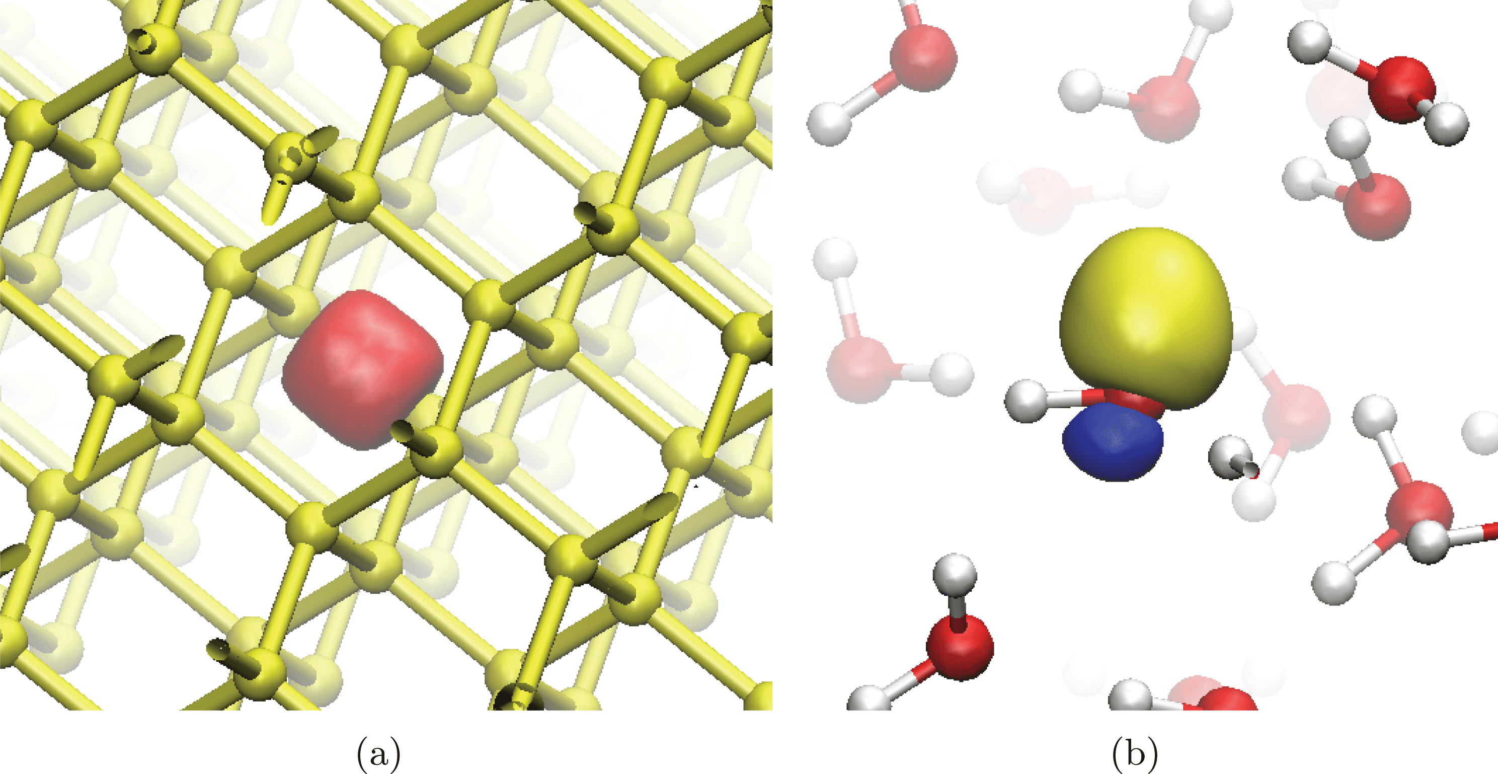
Remarks
Besides using Löwdin transformation, the gauge matrix
 $U$
can also be directly identified from the QRCP (4.6) via a simple choice
 $U=Q$
. This in fact corresponds to another orthogonalization method called the Cholesky-QR factorization, and in this context the Cholesky decomposition can be performed explicitly or implicitly (Golub and Van Loan Reference Golub and Van Loan2013, Damle et al.
Reference Damle, Lin and Ying2017). Numerical results indicate that the two orthogonalization methods have comparable performance. However, the Löwdin transformation can be better when the system has certain spatial symmetries, and can be more easily generalized to periodic crystals.
The numerical methods for finding localized orbitals from the set of occupied orbitals of an insulating systems can be directly generalized to any set of eigenvalues in a given energy interval
 ${\mathcal{I}}$
satisfying the band isolation condition:
 $$\begin{eqnarray}\inf _{\unicode[STIX]{x1D700}_{i}\in {\mathcal{I}},\unicode[STIX]{x1D700}_{i^{\prime }}\notin {\mathcal{I}}}|\unicode[STIX]{x1D700}_{i}-\unicode[STIX]{x1D700}_{i^{\prime }}|:=\unicode[STIX]{x1D700}_{g}>0.\end{eqnarray}$$
When this condition is violated (i.e.
 $\unicode[STIX]{x1D700}_{g}=0$
), the eigenvalues in
 ${\mathcal{I}}$
become entangled. Entangled eigenvalues appear ubiquitously in metallic systems, and also in insulating systems when conduction bands or a selected range of valence bands are considered. The problem now becomes significantly more difficult: to identify a subspace
 ${\mathcal{V}}_{w}$
that admits a localized basis, and to construct such a basis.
The most widely used method to construct localized functions in this scenario is a disentanglement procedure (Souza, Marzari and Vanderbilt Reference Souza, Marzari and Vanderbilt2001). However, the result of the disentanglement procedure may depend sensitively on the initial guess. Often, detailed knowledge of the underlying physical system is required to obtain physically meaningful results. The SCDM method has been extended to handle systems with an entangled band structure in a more robust way (Damle and Lin Reference Damle and Lin2018, Damle, Levitt and Lin Reference Damle, Levitt and Lin2019), using QRCP for a set of ‘quasi’ density matrices. Figure 4.2 demonstrates that the extended SCDM algorithm can accurately interpolate the band structure of graphene, even when zooming in on the region near the Dirac point.
(Credit: Damle and Lin Reference Damle and Lin2018.) Wannier interpolation with SCDM for the band structure for graphene (a) below the Fermi energy and (b) near the Dirac point. Direct calculation (red lines) and SCDM-based Wannier interpolation (blue circles). Here the chemical potential
 $\unicode[STIX]{x1D707}=-2.5$
eV,
 $\unicode[STIX]{x1D70E}=4.0$
eV, and we use a
 $12\times 12\times 1$
 $\mathbf{k}$
-grid to construct the Wannier functions.
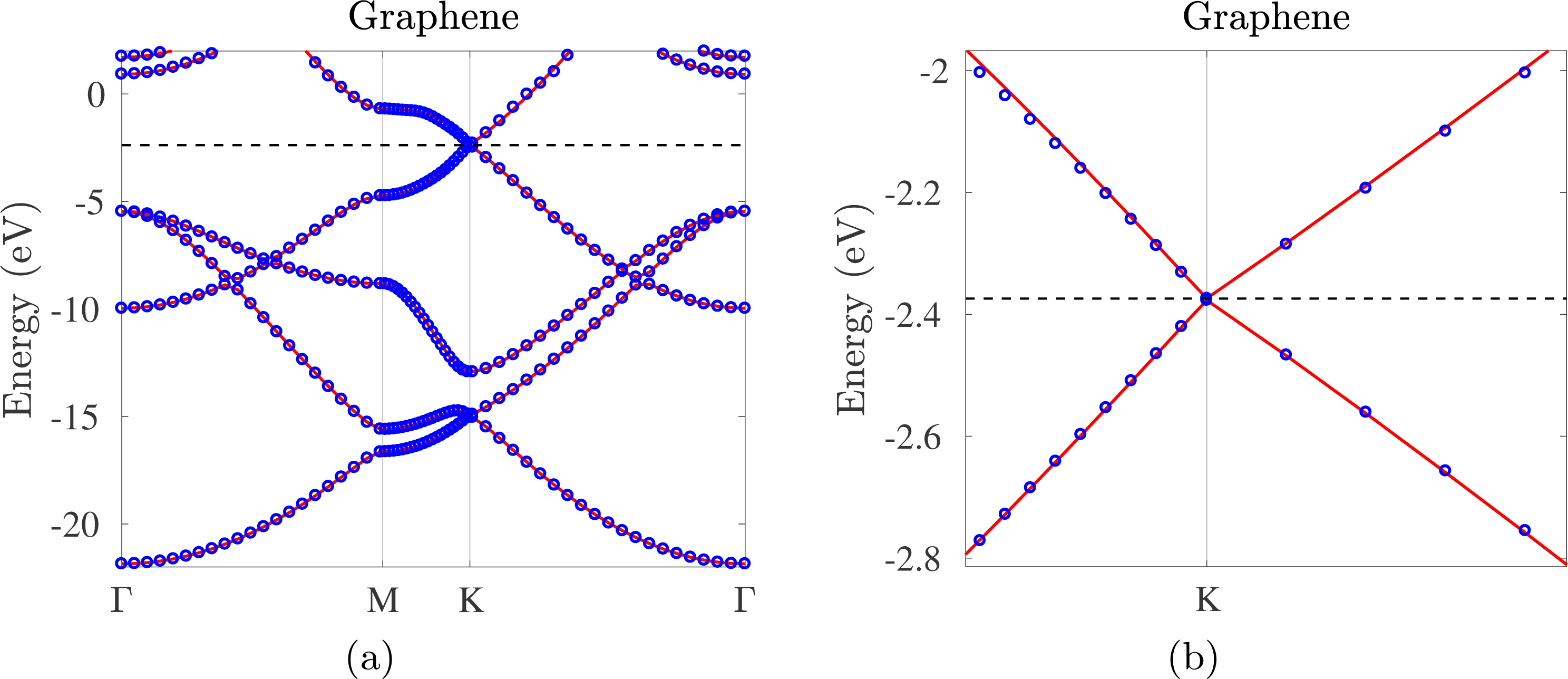
4.4 Interpolative separable density fitting method
Kohn–Sham DFT calculations with rung-4 functionals and beyond often require computing quantities related to the pair product of orbitals, in the form
 $\{\unicode[STIX]{x1D711}_{i}^{\ast }(\mathbf{r})\unicode[STIX]{x1D713}_{j}(\mathbf{r})\}_{i,j=1}^{N}$
. Below we present a technique called interpolative separable density fitting (ISDF) (Lu and Ying Reference Lu and Ying2015, Reference Lu and Ying2016), which allows us to reduce the number of pairs from
 $O(N^{2})$
to
 $O(N)$
in general. This can be used to reduce the cost of rung-4 functional calculations with a large basis set (Hu, Lin and Yang Reference Hu, Lin and Yang2017a
, Dong, Hu and Lin Reference Dong, Hu and Lin2018) (see Section 6.1), as well as RPA correlation energy calculations (Lu and Thicke Reference Lu and Thicke2017a
) (see Section 6.3). It has also been shown to be useful in other contexts such as large-scale phonon calculations (Lin, Xu and Ying Reference Lin, Xu and Ying2017).
To see why it is possible to find a compressed representation of the pair products, let us consider a real-space representation. Note that the number of grid points
 $N_{g}$
to represent the orbital pairs scales linearly with respect to
 $N$
. Hence, as
 $N$
increases, the number of orbital pairs will eventually exceed
 $N_{g}$
. This suggests that the numerical rank of
 $\{\unicode[STIX]{x1D711}_{i}^{\ast }\unicode[STIX]{x1D713}_{j}\}$
, viewed as a matrix of size
 $N_{g}\times N^{2}$
, must scale asymptotically as
 $O(N)$
. On the analytic level, consider the first
 $N$
eigenfunctions
 $\{\unicode[STIX]{x1D713}_{i}\}$
,
 $i=1,\ldots ,N$
of an effective Hamiltonian on a compact domain or closed manifold. Lu, Sogge and Steinerberger (Reference Lu, Sogge and Steinerberger2018) proved that for any
 $\unicode[STIX]{x1D716}$
there exists a subspace
 $B_{N}$
of dimension
 $O_{\unicode[STIX]{x1D6FF}}(\unicode[STIX]{x1D716}^{-\unicode[STIX]{x1D6FF}}N^{1+\unicode[STIX]{x1D6FF}})$
such that
 $$\begin{eqnarray}\Vert \unicode[STIX]{x1D713}_{i}\unicode[STIX]{x1D713}_{j}-\unicode[STIX]{x1D6F1}_{B_{N}}(\unicode[STIX]{x1D713}_{i}\unicode[STIX]{x1D713}_{j})\Vert _{L^{2}}\leq \unicode[STIX]{x1D716},\end{eqnarray}$$
where
 $\unicode[STIX]{x1D6FF}$
is an arbitrary positive constant. In other words, we can approximate the
 $N^{2}$
pair products of eigenfunctions with almost
 $O(N)$
auxiliary basis functions, regardless of the discretization level.
Motivated by the above observation, the ISDF method uses the following compression format:
 $$\begin{eqnarray}\unicode[STIX]{x1D711}_{i}^{\ast }(\mathbf{r})\unicode[STIX]{x1D713}_{j}(\mathbf{r})\approx \mathop{\sum }_{\unicode[STIX]{x1D707}=1}^{N_{\unicode[STIX]{x1D707}}}\unicode[STIX]{x1D711}_{i}^{\ast }(\hat{\mathbf{r}}_{\unicode[STIX]{x1D707}})\unicode[STIX]{x1D713}_{j}(\hat{\mathbf{r}}_{\unicode[STIX]{x1D707}})\unicode[STIX]{x1D701}_{\unicode[STIX]{x1D707}}(\mathbf{r}).\end{eqnarray}$$
Here
 $\{\hat{\mathbf{r}}_{\unicode[STIX]{x1D707}}\}_{\unicode[STIX]{x1D707}=1}^{N_{\unicode[STIX]{x1D707}}}$
is a subset of real-space grid points
 $\{\mathbf{r}_{i}\}_{i=1}^{N_{g}}$
on which the orbitals are evaluated. We will refer to
 $\{\hat{\mathbf{r}}_{\unicode[STIX]{x1D707}}\}_{\unicode[STIX]{x1D707}=1}^{N_{\unicode[STIX]{x1D707}}}$
as the interpolation points, and
 $\{\unicode[STIX]{x1D701}_{\unicode[STIX]{x1D707}}(\mathbf{r})\}_{\unicode[STIX]{x1D707}=1}^{N_{\unicode[STIX]{x1D707}}}$
sampled on
 $\{\mathbf{r}_{i}\}_{i=1}^{N_{g}}$
the interpolation vectors.
The ISDF decomposition can also be understood from the perspective of interpolation. Let
 $\{\hat{\mathbf{r}}_{\unicode[STIX]{x1D707}}\}$
denote a set of grid points in real space, and let
 $\unicode[STIX]{x1D701}_{\unicode[STIX]{x1D707}}(\mathbf{r})$
be the Lagrange interpolation function on these grid points satisfying
 $$\begin{eqnarray}\unicode[STIX]{x1D701}_{\unicode[STIX]{x1D707}}(\hat{\mathbf{r}}_{\unicode[STIX]{x1D707}^{\prime }})=\left\{\begin{array}{@{}ll@{}}1\quad & \unicode[STIX]{x1D707}=\unicode[STIX]{x1D707}^{\prime },\\ 0\quad & \text{otherwise}.\end{array}\right.\end{eqnarray}$$
Then the ISDF decomposition would become sufficiently accurate as one systematically refines the set
 $\{\hat{\mathbf{r}}_{\unicode[STIX]{x1D707}}\}_{\unicode[STIX]{x1D707}=1}^{N_{\unicode[STIX]{x1D707}}}$
. In the worst case, all grid points need to be selected and
 $N_{\unicode[STIX]{x1D707}}=N_{g}$
. However, numerical evidence and analytical results suggest that the decomposition often becomes sufficiently accurate when
 $N_{\unicode[STIX]{x1D707}}\ll N_{g}$
, especially when both
 $\{\unicode[STIX]{x1D711}_{i}(\mathbf{r})\}$
and
 $\{\unicode[STIX]{x1D713}_{i}(\mathbf{r})\}$
consist of functions that are sufficiently smooth.
We first assume that the interpolation points
 $\{\hat{\mathbf{r}}_{\unicode[STIX]{x1D707}}\}$
are given, and discuss how to find the interpolation vectors. Define
 $$\begin{eqnarray}{\{Z_{ij}(\mathbf{r}):=\unicode[STIX]{x1D711}_{i}^{\ast }(\mathbf{r})\unicode[STIX]{x1D713}_{j}(\mathbf{r})\}}_{1\leq i\leq N,1\leq j\leq N},\end{eqnarray}$$
and equation (4.13) can be written as
 $$\begin{eqnarray}Z=\unicode[STIX]{x1D6E9}C,\end{eqnarray}$$
where each column of
 $Z$
is defined by equation (4.15) sampled on real-space grids
 $\{\mathbf{r}_{i}\}_{i=1}^{N_{g}}$
.
 $\unicode[STIX]{x1D6E9}=[\unicode[STIX]{x1D701}_{1},\unicode[STIX]{x1D701}_{2},\ldots ,\unicode[STIX]{x1D701}_{N_{\unicode[STIX]{x1D707}}}]$
contains the interpolating vectors, and each column of
 $C$
with a multi-index
 $(i,j)$
is given by
 $$\begin{eqnarray}[\unicode[STIX]{x1D711}_{i}^{\ast }(\hat{\mathbf{r}}_{1})\unicode[STIX]{x1D713}_{j}(\hat{\mathbf{r}}_{1}),\ldots ,\unicode[STIX]{x1D711}_{i}^{\ast }(\hat{\mathbf{r}}_{\unicode[STIX]{x1D707}})\unicode[STIX]{x1D713}_{j}(\hat{\mathbf{r}}_{\unicode[STIX]{x1D707}}),\ldots ,\unicode[STIX]{x1D711}_{i}^{\ast }(\hat{\mathbf{r}}_{N_{\unicode[STIX]{x1D707}}})\unicode[STIX]{x1D713}_{j}(\hat{\mathbf{r}}_{N_{\unicode[STIX]{x1D707}}})]^{\top }.\end{eqnarray}$$
Equation (4.16) is an over-determined linear systems with respect to the interpolation vectors
 $\unicode[STIX]{x1D6E9}$
. One possible way to solve the over-determined system is to impose the Galerkin condition
 $$\begin{eqnarray}ZC^{\ast }=\unicode[STIX]{x1D6E9}CC^{\ast }.\end{eqnarray}$$
It follows that the interpolating vectors can be obtained from
 $$\begin{eqnarray}\unicode[STIX]{x1D6E9}=ZC^{\ast }(CC^{\ast })^{-1}.\end{eqnarray}$$
Note that the solution given by equation (4.18) is a least-squares approximation to the solution of equation (4.13).
It may appear that the cost of matrix–matrix multiplications
 $ZC^{\ast }$
and
 $CC^{\ast }$
scales as
 $O(N^{4})$
, because the size of
 $Z$
is
 $N_{g}\times N^{2}$
and the size of
 $C$
is
 $N_{\unicode[STIX]{x1D707}}\times N^{2}$
. However, both multiplications can be carried out with fewer operations due to the separable structure of
 $Z$
and
 $C$
, and the computational complexity of computing the interpolation vectors is therefore
 $O(N^{3})$
.
In order to optimize the set of interpolation points, a general strategy is to use the QR factorization with column pivoting (QRCP), as in the case of the SCDM method in Section 4.3. Pseudocode for the ISDF algorithm is given in Algorithm 4.

To demonstrate the interpolation points selected from the QRCP procedure, we consider a water molecule, with
 $N_{\unicode[STIX]{x1D707}}=8$
interpolation points distributed in real space (see Figure 4.3). The choice of interpolation points agrees with chemical intuition: the locations of these points are consistent with the distribution of the electron density, and the points are relatively well separated, so that the set of interpolation vectors do not become linearly dependent.
(Credit: Hu et al.
Reference Hu, Lin and Yang2017a
.) (a) The electron density (yellow isosurfaces) and (b) the interpolation points (green squares)
 $\{\hat{\mathbf{r}}_{\unicode[STIX]{x1D707}}\}_{\unicode[STIX]{x1D707}=1}^{N_{\unicode[STIX]{x1D707}}}$
(
 $N_{\unicode[STIX]{x1D707}}$
= 8) selected from the real-space grid points
 $\{\mathbf{r}_{i}\}_{i=1}^{N_{g}}$
(
 $N_{g}$
= 66
 $^{3}$
) for a water molecule in a 10 Å
 $\times$
10 Å
 $\times$
10 Å box. The white and red balls denote hydrogen and oxygen atoms, respectively.
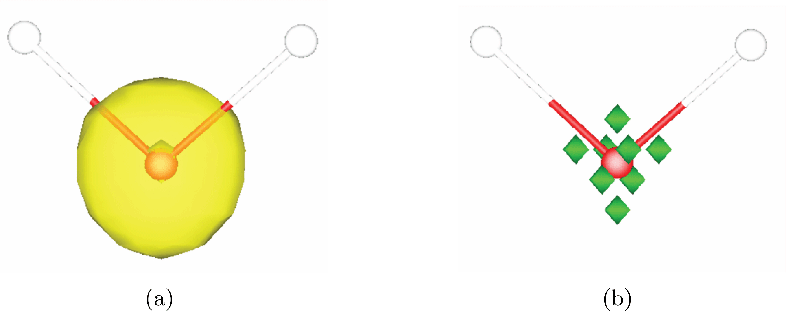
The disadvantage of using equation (4.16) directly is that the storage requirement for the matrix
 $Z$
is
 $O(N^{3})$
and the computational cost associated with a standard QRCP procedure is
 $O(N^{4})$
. One possibility is to lower the cost of QRCP by using a random matrix to subsample columns of the matrix
 $Z$
to form a smaller matrix
 $\widetilde{Z}$
of size
 $N_{g}\times \widetilde{N}_{\unicode[STIX]{x1D707}}$
, where
 $\widetilde{N}_{\unicode[STIX]{x1D707}}$
is only slightly larger than
 $N_{\unicode[STIX]{x1D707}}$
(Lu and Ying Reference Lu and Ying2015, Reference Lu and Ying2016). The reduced matrix size allows the computational cost of the QRCP procedure to be reduced to
 $O(N^{3})$
. Since the QRCP algorithm has been implemented in standard linear algebra software packages such as LAPACK and ScaLAPACK, the implementation and parallelization of ISDF is then relatively straightforward.
Another possibility for choosing interpolation points is to use a heuristic strategy. Note that an effective choice of the set of interpolation points should satisfy the following two conditions.
(1) The distribution of the interpolation points should roughly follow the distribution of the electron density. In particular, there should be more points when the electron density is high, and fewer or even zero points if the electron density is very low.
(2) The interpolation points should not be very close to each other. Otherwise matrix rows represented by the interpolation points are nearly linearly dependent, and the matrix formed by the interpolation vectors become highly ill-conditioned.
The QRCP procedure satisfies both (i) and (ii) simultaneously. On the other hand, the conditions above can also be satisfied via a much simpler centroidal Voronoi tessellation (CVT) procedure applied to a weight vector, such as the electron density. More specifically, in the centroidal Voronoi tessellation (CVT) approach, we may partition the grid points in the global domain into
 $N_{\unicode[STIX]{x1D707}}$
Voronoi cells. The interpolation points can then be simply chosen to be the centroids corresponding to each cell. The CVT procedure can be effectively implemented through a K-Means algorithm (MacQueen Reference MacQueen1967). Besides reduction of the computational cost, the use of a K-Means algorithm also produces a smoother potential energy surface, particularly in the context of ab initio molecular dynamics. We refer to Dong et al. (Reference Dong, Hu and Lin2018) for more details of this approach.
Remarks
As in the SCDM method in Section 4.3, the ISDF method also relies on the real-space representation and smoothness of the orbitals. When small basis sets such as Gaussian-type orbitals are used, one possible way of using ISDF is to first interpolate the orbitals onto a real-space grid. However, in the context of all-electron calculations, the grid size needed to reach chemical accuracy can be exceedingly large. Hence in the quantum chemistry literature, the compression is often performed using the density fitting method (a.k.a. resolution of identity) (Weigend Reference Weigend2002, Ren et al.
Reference Ren, Rinke, Blum, Wieferink, Tkatchenko, Sanfilippo, Reuter and Scheffler2012a
), applied to the basis functions
 $\{\unicode[STIX]{x1D719}_{p}\}_{p=1}^{N_{b}}$
directly. More specifically, density fitting seeks the following decomposition:
 $$\begin{eqnarray}\unicode[STIX]{x1D719}_{p}^{\ast }(\mathbf{r})\unicode[STIX]{x1D719}_{q}(\mathbf{r})\approx \mathop{\sum }_{\unicode[STIX]{x1D707}=1}^{N_{\unicode[STIX]{x1D707}}}C_{\unicode[STIX]{x1D707}}^{pq}\unicode[STIX]{x1D701}_{\unicode[STIX]{x1D707}}(\mathbf{r}),\end{eqnarray}$$
where the number of auxiliary functions
 $N_{\unicode[STIX]{x1D707}}$
is expected to be much smaller than the number of pairs
 $N_{b}^{2}$
. The density fitting method can be viewed as an approximate solution to the singular value decomposition (SVD) of the matrix formed by the product of pairs of orbitals.
We remark that there is an important technical difference between ISDF and standard density fitting methods. In ISDF, the interpolation points
 $\{\hat{\mathbf{r}}_{\unicode[STIX]{x1D707}}\}$
are chosen first, and the auxiliary functions
 $\{\unicode[STIX]{x1D701}_{\unicode[STIX]{x1D707}}\}$
are decided accordingly via a least-squares procedure. The interpolation coefficients in ISDF are obtained directly with a factorized form
 $$\begin{eqnarray}C_{\unicode[STIX]{x1D707}}^{pq}=\unicode[STIX]{x1D719}_{p}^{\ast }(\hat{\mathbf{r}}_{\unicode[STIX]{x1D707}})\unicode[STIX]{x1D719}_{q}(\hat{\mathbf{r}}_{\unicode[STIX]{x1D707}}).\end{eqnarray}$$
In standard density fitting methods, the auxiliary functions are often chosen a priori, and part of the reason is to facilitate the computation of the two-electron integrals in subsequent calculations. The interpolation coefficients
 $\{C_{\unicode[STIX]{x1D707}}^{pq}\}$
are then determined via a least-squares procedure. Since
 $\{C_{\unicode[STIX]{x1D707}}^{pq}\}$
is generally a dense three-way tensor, the computational cost of density fitting scales generally as
 $O(N^{4})$
unless additional locality constraints are enforced (Ren et al.
Reference Ren, Rinke, Blum, Wieferink, Tkatchenko, Sanfilippo, Reuter and Scheffler2012a
).
Another technique to reduce the cost of the density fitting method is the tensor hypercontraction (THC) method (Parrish, Hohenstein, Martínez and Sherrill Reference Parrish, Hohenstein, Martínez and Sherrill2012, Reference Parrish, Hohenstein, Martínez and Sherrill2013), which is closely related to the ISDF method. Conceptually, THC aims at compressing the two-electron integrals directly, without going through intermediate decomposition of the form (4.19) with separable coefficients as in (4.20). However, since the two-electron integrals is a four-way tensor to start with, the computational cost associated with the THC decomposition can be
 $O(N^{5})$
. Once the decomposition is obtained, the THC format can then be used to reduce the cost of post-Hartree–Fock calculations, such as MP2 and coupled cluster theories.
5 Evaluation of the Kohn–Sham map: semi-local functional
When solving Kohn–Sham DFT using the self-consistent field iteration, the most computationally expensive step is the evaluation of the Kohn–Sham map. For a given effective Hamiltonian at the current iteration, one needs to determine the electronic structure, in the form of occupied orbitals or the electron density. In this section we discuss the evaluation of the Kohn–Sham map for semi-local functionals. Given an effective Hamiltonian as a matrix, the straightforward way to obtain the corresponding density is to use conventional direct diagonalization (see Section 4.1) or iterative diagonalization (see Section 4.2) algorithms to obtain the low-lying eigenfunctions and then the electron density. These methods inherently display cubic scaling with respect to the system size, and become computationally expensive or even infeasible for large-scale systems.
To reduce the computational cost, it is important to realize that we require only the electron density in the Kohn–Sham map, but not the eigenfunctions or eigenvalues. More efficient algorithms can thus be developed for the Kohn–Sham map. In Section 5.1, we review filtering methods that are iterative methods not trying to converge to each individual eigenvector, but instead to the occupied subspace, which can often be much more efficient than traditional iterative solvers for eigenvalue problems.
Since we do not need each individual eigenvector, we can use an alternative representation for the occupied subspace, such as the density matrix or localized orbitals. By exploiting the sparsity, it is even possible to achieve linear scaling for insulating systems. We will review such methods in Section 5.2. While linear scaling methods are in principle desirable, it is often challenging to control their accuracy unless the system has a relatively large gap. The pole expansion and selected inversion method (PEXSI) has been developed as a reduced scaling method that yields accurate approximation for general systems, which will be discussed in Section 5.3.
5.1 Filtering methods
Instead of using Krylov-type methods to approximate the low-lying eigenmodes, one can also identify the low eigenmodes by evaluating an appropriate polynomial of the Hamiltonian
 $H$
. The main criterion for choosing such a polynomial
 $p(z)$
is that it should maximize the magnitudes at the eigenvalues
 $\unicode[STIX]{x1D706}_{1},\ldots ,\unicode[STIX]{x1D706}_{N}$
and at the same time minimize the magnitudes at the eigenvalues
 $\unicode[STIX]{x1D706}_{N+1},\ldots ,\unicode[STIX]{x1D706}_{N_{b}}$
. One of the most popular choices is the shifted-and-scaled Chebyshev polynomial
 $P_{k}(z)$
that maps the standard interval
 $[-1,1]$
to
 $[\unicode[STIX]{x1D706}_{N+1},\unicode[STIX]{x1D706}_{N_{b}}]$
, where the subscript
 $k$
denotes the degree of this Chebyshev polynomial (Zhou, Saad, Tiago and Chelikowsky Reference Zhou, Saad, Tiago and Chelikowsky2006). The absolute values of Chebyshev polynomials are bounded by
 $1$
within the interval
 $[-1,1]$
and grow rapidly outside this interval. Hence the shifted-and-scaled Chebyshev polynomial
 $P_{k}(z)$
only amplifies the occupied states of the
 $H$
. In practice, one does not know a priori the values of
 $\unicode[STIX]{x1D706}_{N+1}$
and
 $\unicode[STIX]{x1D706}_{N_{b}}$
. These values need to be estimated from the Kohn–Sham Hamiltonian (e.g. applying a few steps of the Lanczos iteration (Zhou, Chelikowsky and Saad Reference Zhou, Chelikowsky and Saad2014)), and also updated on the fly. When applying the Chebyshev filtering algorithm, we also often choose the number of states
 $N_{s}$
to be slightly larger than the number of occupied orbitals
 $N$
, to accelerate the convergence. Pseudocode for the Chebyshev filtering algorithm is shown in Algorithm 5.

The Chebyshev filtering algorithm is presented here as a diagonalization procedure, that is, one iterates until the low-lying eigenvalues converge. However, in many implementations, due to the existence of the outer SCF iteration, one often performs a handful of iterations (applying Chebyshev polynomials and orthonormalization) and accepts whatever improvement it produces. Sometimes even a single iteration per outer SCF iteration may be sufficient. An equivalent view is that it combines the outer SCF loop with the inner diagonalization loop, without performing accurate diagonalization. For many problems, such a combination does not increase the number of outer SCF iterations and hence may significantly reduce the overall running time.
Application of the Chebyshev polynomial to all occupied states scales as
 $O(N_{b}N)$
. For large problems, the most expensive step is the solution of the Rayleigh–Ritz problem in step 4 (also called the subspace diagonalization step) of Algorithm 5, which scales as
 $O(N^{3})$
. Although the cubic scaling cannot be avoided in the filtering-based approaches, the prefactors can be significantly reduced by the following complementary subspace method (Banerjee et al.
Reference Banerjee, Lin, Suryanarayana, Yang and Pask2018).
In the Chebyshev filtering approach, the density matrix is computed as
 $$\begin{eqnarray}P=Y\tilde{P}Y^{\ast },\end{eqnarray}$$
where
 $\tilde{P}\in \mathbb{R}^{N_{s}\times N_{s}}$
is the projected density matrix, with its eigenvalues given by the occupation numbers
 $\{f_{i}\}_{i=1}^{N_{s}}$
, evaluated according to the Fermi–Dirac distribution in equation (2.66), for example (we switch to the finite temperature case here). Since
 $N_{s}$
is only slightly larger than
 $N$
, most of the occupation numbers are approximately equal to
 $1$
. We denote states
 $1$
to
 $N_{1}$
as those with occupation numbers equal to
 $1$
within numerical tolerance. The remaining states, from
 $N_{1}+1$
to
 $N_{s}$
, have occupation numbers less than
 $1$
. Let
 $N_{t}$
be the number of these fractionally occupied states, i.e.
 $N_{t}=N_{s}-N_{1}$
. The eigenvectors of the projected density matrix are
 $\{\tilde{\unicode[STIX]{x1D713}}_{i}\}_{i=1}^{N_{s}}$
, and we may rewrite the expression for the projected density matrix as
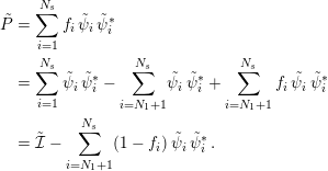 $$\begin{eqnarray}\displaystyle \tilde{P} & = & \displaystyle \mathop{\sum }_{i=1}^{N_{s}}f_{i}\,\tilde{\unicode[STIX]{x1D713}}_{i}\,\tilde{\unicode[STIX]{x1D713}}_{i}^{\ast }\,\nonumber\\ \displaystyle & = & \displaystyle \mathop{\sum }_{i=1}^{N_{s}}\tilde{\unicode[STIX]{x1D713}}_{i}\,\tilde{\unicode[STIX]{x1D713}}_{i}^{\ast }-\mathop{\sum }_{i=N_{1}+1}^{N_{s}}\!\tilde{\unicode[STIX]{x1D713}}_{i}\,\tilde{\unicode[STIX]{x1D713}}_{i}^{\ast }+\mathop{\sum }_{i=N_{1}+1}^{N_{s}}f_{i}\,\tilde{\unicode[STIX]{x1D713}}_{i}\,\tilde{\unicode[STIX]{x1D713}}_{i}^{\ast }\nonumber\\ \displaystyle & = & \displaystyle \tilde{{\mathcal{I}}}-\mathop{\sum }_{i=N_{1}+1}^{N_{s}}(1-f_{i})\,\tilde{\unicode[STIX]{x1D713}}_{i}\,\tilde{\unicode[STIX]{x1D713}}_{i}^{\ast }\,.\end{eqnarray}$$
In equation (5.2) above,
 $\tilde{{\mathcal{I}}}$
is the identity matrix of dimension
 $N_{s}\times N_{s}$
. That the first term of equation (5.2) is the identity matrix follows from the resolution of the identity. Hence, if the
 $N_{t}$
top eigenvectors
 $\tilde{\unicode[STIX]{x1D713}_{i}}$
and corresponding occupation numbers
 $f_{i}$
are known, the projected density matrix
 $\tilde{P}$
may be computed. Thus, instead of determining the full
 $N_{s}\times N_{s}$
set of vectors, we need to determine only an extremal block of vectors (of dimension
 $N_{s}\times N_{t}$
), corresponding to the states
 $i=N_{1}+1$
to
 $N_{s}$
.
Moreover, physical quantities such as the electron density, energy, entropy and atomic force can all be computed by knowing only the top eigenstates. These eigenstates can be efficiently evaluated via several Chebyshev polynomial filtering steps applied to the projected Hamiltonian matrix
 $\tilde{H}$
. Using this complementary subspace strategy with two levels of Chebyshev filtering (CS2CF), for insulating systems, the Rayleigh–Ritz step may be avoided altogether. For metallic systems, the cost of the Rayleigh–Ritz step can also be significantly reduced. Table 5.1 shows that the CS2CF strategy can be applied to insulating and metallic systems with
 $O(10^{4})$
atoms and efficiently parallelized over
 $O(10^{4})$
computational cores. The wall clock time to solution can be more than an order of magnitude faster than parallel dense diagonalization methods such as ELPA for large systems.
(Credit: Banerjee et al. Reference Banerjee, Lin, Suryanarayana, Yang and Pask2018.) Wall clock times for one SCF iteration large systems using the CS2CF strategy in DGDFT.
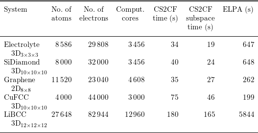
Remarks
The idea of filtering the Hamiltonian matrix also appears in the spectral slicing approach (Zhang, Smith, Sternberg and Zapol Reference Zhang, Smith, Sternberg and Zapol2007, Polizzi Reference Polizzi2009, Schofield, Chelikowsky and Saad Reference Schofield, Chelikowsky and Saad2012, Aktulga et al.
Reference Aktulga, Lin, Haine, Ng and Yang2014). The basic idea is to project matrix functions
 $f_{i}(H)$
to a set of orbitals, where
 $f_{i}(\cdot )$
can be polynomials or rational functions approximately supported only on a small segment
 ${\mathcal{I}}_{i}$
. Then one may perform diagonalization methods to compute the eigenvalues restricted to the segment. Finally, the eigenvalues obtained from different segments of the spectrum are merged together. The spectral splicing approach is naturally suited to massive parallelization. Each core or multiple cores together may focus on calculations associated with one segment, and may significantly reduce the wall clock time. Note that spectral slicing methods may involve multiple parameters, such as the partitioning strategy of the spectrum, the degrees of filtering polynomials, and the merging strategy of different segments of the spectrum. Finding an efficient and robust strategy to determine these parameters is still an active research area.
5.2 Linear scaling methods
Direct diagonalization and iterative methods for solving the Kohn–Sham eigenvalue problem scale cubically with system size. The cubic scaling is the bottleneck for electronic structure calculations of large systems. When a set of localized basis functions such as atomic orbitals and real-space representation are used, the resulting Hamiltonian matrix from the Kohn–Sham eigenvalue problem is localized. For insulating systems, the density matrix is localized and there exist localized representations – Wannier functions – for the subspace spanned by the occupied orbitals, as discussed in Section 4.3. One might hope to obtain the electronic structure, in the form of either a density matrix or localized orbitals, with a computation cost that scales linearly with system size. Such algorithms are referred to as ‘linear scaling methods’. Many algorithms have been proposed and investigated over the past
 $30$
years.
To achieve linear scaling, one needs to bypass the diagonalization of the Kohn–Sham Hamiltonian matrix. The crucial observation is that in the self-consistent iteration, we do not need full information on the eigenvectors. Thus, it is possible to reformulate the Kohn–Sham eigenvalue problem in a way that allows us to exploit the locality of the density matrix or localized orbitals to reduce computational complexity. In the following, we review a few representative linear scaling methods. While the list does not cover all algorithms developed in the literature, the discussion covers most of the existing ideas and strategies to achieve linear scaling. We refer readers to Goedecker (Reference Goedecker1999) and Bowler and Miyazaki (Reference Bowler and Miyazaki2012) for a more extensive review of linear scaling methods.
5.2.1 Divide-and-conquer method
The divide-and-conquer method proposed by Weitao Yang (Yang Reference Yang1991a ,Reference Yang b ) is the first linear scaling method proposed in the literature for Kohn–Sham DFT. The idea of divide-and-conquer is to divide the physical system into several subsystems. The effective Hamiltonian for each subsystem is then solved separately, and the electron density of the whole system is obtained by merging the results of the subsystems together.
The divide-and-conquer method for each SCF step is described in Algorithm 6. Here a real-space representation is assumed. The divide-and-conquer method was originally developed for discretization using localized basis functions (Yang Reference Yang1991a ,Reference Yang b ), in which case the algorithm is slightly different but shares the same spirit.

The divide-and-conquer method relies on the near-sightedness of the electron matter, as formulated by Kohn (Reference Kohn1996). Roughly speaking, the dependence of electron density at
 $\mathbf{r}$
on the effective potential at
 $\mathbf{r}^{\prime }$
is negligible when
 $|\mathbf{r}-\mathbf{r}^{\prime }|$
is large. Hence, in the interior of the domain
 $\unicode[STIX]{x1D6FA}_{\unicode[STIX]{x1D705}}$
, the electron density corresponding to the Hamiltonian
 $H$
is well approximated by that of the truncated Hamiltonian
 $H_{\unicode[STIX]{x1D705}}$
, since
 $H$
agrees with
 $H_{\unicode[STIX]{x1D705}}$
inside
 $\unicode[STIX]{x1D6FA}_{\unicode[STIX]{x1D705}}$
. To make this work, besides requiring that the original system
 $H$
is insulating, we also require that the truncated system
 $H_{\unicode[STIX]{x1D705}}$
does not destroy the energy gap (which could happen in practice, e.g. for heterogeneous systems). See Chen and Lu (Reference Chen and Lu2016) for a mathematical analysis of the divide-and-conquer method, based on the analysis tools developed in E and Lu (Reference E and Lu2011).
Further developments of the divide-and-conquer method and related domain decomposition type method can be found in Yang and Lee (Reference Yang and Lee1995), Wang, Zhao and Meza (Reference Wang, Zhao and Meza2008), Zhao, Meza and Wang (Reference Zhao, Meza and Wang2008), Barrault, Cancès, Hager and Le Bris (Reference Barrault, Cancès, Hager and Le Bris2007) and Bencteux et al. (Reference Bencteux, Barrault, Cancès, Hager, Le Bris, Glowinski and Neittaanmäki2008). A great advantage of the method lies in the intrinsic parallelism of the computation for each subsystem, which has been utilized for large-scale calculations with more than
 $10^{6}$
atoms and
 $10^{12}$
electronic degrees of freedom (Kobayashi and Nakai Reference Kobayashi and Nakai2009, Ohba et al.
Reference Ohba, Ogata, Kouno, Tamura and Kobayashi2012, Shimojo, Kalia, Nakano and Vashishta Reference Shimojo, Kalia, Nakano and Vashishta2008, Shimojo et al.
Reference Shimojo, Ohmura, Nakano, Kalia and Vashishta2011).
The divide-and-conquer method is based on separating the total computational domain into smaller ones and solving the eigenvalue problem for each subdomain. There are other linear scaling methods based on reformulations of the Kohn–Sham problems to bypass the eigenvalue problem, as we will discuss below.
5.2.2 Orbital minimization methods
According to the Courant–Fisher variational principle, the first
 $N$
eigenvectors of the discretized Hamiltonian matrix
 $H$
can be found by solving
 $$\begin{eqnarray}E=\min _{X,\;X^{\ast }X=I}\operatorname{Tr}(X^{\ast }HX),\end{eqnarray}$$
where
 $X\in \mathbb{C}^{N_{b}\times N}$
is the matrix of discretized orbitals. The orthogonality constraint
 $X^{\ast }X=I$
is a bottleneck for linear scaling, as the cost of both the Gram–Schmidt orthogonalization and the Rayleigh–Ritz step scale cubically with respect to the system size.
The orbital minimization method (OMM) (Mauri, Galli and Car Reference Mauri, Galli and Car1993, Ordejón, Drabold, Grumbach and Martin Reference Ordejón, Drabold, Grumbach and Martin1993, Mauri and Galli Reference Mauri and Galli1994, Ordejón, Drabold, Martin and Grumbach Reference Ordejón, Drabold, Martin and Grumbach1995) is based instead on an unconstrained variational formulation,
 $$\begin{eqnarray}E=\min _{X}\operatorname{Tr}((2I-X^{\ast }X)(X^{\ast }(H-\unicode[STIX]{x1D700}_{ max})X)),\end{eqnarray}$$
where
 $\unicode[STIX]{x1D700}_{\max }$
is an upper bound of the eigenvalue of
 $H$
. The shift of the Hamiltonian by
 $-\unicode[STIX]{x1D700}_{\max }$
makes all its eigenvalues negative, so the objective function is bounded from below, while it does not affect the eigenvectors of
 $H$
.
While the OMM variational problem looks rather different from (5.3), it can be shown that the global minimizer
 $X$
of (5.4) spans the eigenspace of the lowest
 $N$
eigenvalues of
 $H$
(assuming non-degeneracy) (Mauri et al.
Reference Mauri, Galli and Car1993, Pfrommer, Demmel and Simon Reference Pfrommer, Demmel and Simon1999). In fact, somewhat surprisingly, while the objective function (5.4) is non-convex, it is proved in Lu and Thicke (Reference Lu and Thicke2017b
) that every local minimum of (5.4) is in fact also a global minimum. Thus it suffices for an optimization algorithm to converge locally.
The OMM minimization can be used as an alternative to direct diagonalization, as a way to obtain the Kohn–Sham map. This is implemented in the library libOMM (Corsetti Reference Corsetti2014) with the preconditioned conjugate gradient algorithm.
More commonly, OMM is combined with truncation of the iterates of
 $X$
to achieve linear scaling by only keeping
 $O(1)$
entries for each column of
 $X$
during the iteration (Mauri et al.
Reference Mauri, Galli and Car1993, Ordejón et al.
Reference Ordejón, Drabold, Grumbach and Martin1993). The hope is that the algorithm converges to the localized representation of the occupied space for insulating systems. However, with truncation, the optimization procedure might get stuck. Strategies to alleviate the problem have been proposed, for examplein Kim, Mauri and Galli (Reference Kim, Mauri and Galli1995), Tsuchida (Reference Tsuchida2007), Gao and E (Reference Gao and E2009) and Lu and Thicke (Reference Lu and Thicke2017b
). The OMM is used in the SIESTA package (Soler et al.
Reference Soler, Artacho, Gale, García, Junquera, Ordejón and Sánchez-Portal2002) to achieve linear scaling.
As in OMM, localization and truncation steps can also be combined with other iterative algorithms that only rely on the subspace (rather than individual eigenvectors) to achieve linear scaling. One such algorithm is the localized subspace iteration algorithm (Li and Lu Reference Li and Lu2010, Garcia-Cervera, Lu, Xuan and E Reference Garcia-Cervera, Lu, Xuan and E2009), based on the Chebyshev filtering method (Algorithm 5). The Rayleigh–Ritz step (i.e. step 4 of Algorithm 5) is replaced by a localization and truncation step to maintain sparsity.
5.2.3 Density matrix minimization methods
Besides using orbitals, one can also use the density matrix in the variational approach for linear scaling algorithms. The starting point is the following variational principle in terms of density matrices:
 $$\begin{eqnarray}\displaystyle & & \displaystyle E=\min _{P}\operatorname{Tr}(PH)\nonumber\\ \displaystyle & & \displaystyle \;\text{subject to}~P^{2}=P,P=P^{\ast },\operatorname{Tr}P=N.\end{eqnarray}$$
In the above minimization, the idempotency constraint
 $P^{2}=P$
is not easy to deal with, similar to the orthogonality constraint for orbitals. The idea is to circumvent the constraint by using some alternative variational principles. One such variational principle is
 $$\begin{eqnarray}\displaystyle & & \displaystyle E=\min _{P}E^{\text{DMM}}[P]:=\min _{P}\operatorname{Tr}((3P^{2}-2P^{3})(H-\unicode[STIX]{x1D707}))\nonumber\\ \displaystyle & & \displaystyle \;\text{subject to}~P=P^{\ast },\end{eqnarray}$$
where
 $\unicode[STIX]{x1D707}$
is the chemical potential assumed to be known, whose determination can be done by solving the constraint that
 $\operatorname{Tr}P=N$
(we will further discuss how to determine the chemical potential at the end of Section 5.2.4). Note that in (5.6) we have replaced
 $P$
in the trace term by the polynomial
 $3P^{2}-2P^{3}$
(this is known as the McWeeny purification polynomial, which will be discussed in more detail in Section 5.2.4) and used a constant shift of the Hamiltonian by the chemical potential. To minimize (5.6), one can typically start with an initial guess (e.g.
 $P_{(0)}={\textstyle \frac{1}{2}}I$
) and employ the conjugate gradient method to minimize the energy.
The energy (5.6) is in fact not bounded from below. Let
 $\unicode[STIX]{x1D700}_{i}$
be one of the eigenvalues of
 $H$
that is larger than
 $\unicode[STIX]{x1D707}$
; we can take
 $P=\sum _{i}f_{i}|\unicode[STIX]{x1D713}_{i}\rangle \langle \unicode[STIX]{x1D713}_{i}|$
and send
 $f_{i}\rightarrow \infty$
to make the energy go to
 $-\infty$
. On the other hand, convergence can be proved with particular choices of initial conditions and minimization algorithms. The variation of (5.6) can be computed as
 $$\begin{eqnarray}\unicode[STIX]{x1D6FF}E^{\text{DMM}}=\operatorname{Tr}\biggl[\displaystyle \frac{\unicode[STIX]{x1D6FF}E^{\text{DMM}}}{\unicode[STIX]{x1D6FF}P}\unicode[STIX]{x1D6FF}P\biggr],\end{eqnarray}$$
where
 $$\begin{eqnarray}\displaystyle \frac{\unicode[STIX]{x1D6FF}E^{\text{DMM}}}{\unicode[STIX]{x1D6FF}P}=3(PH+HP-2\unicode[STIX]{x1D707}P)-2(P^{2}H+PHP+HP^{2}-3\unicode[STIX]{x1D707}P^{2}).\end{eqnarray}$$
When
 $P$
commutes with
 $H$
, equation (5.8) can be simplified as
 $$\begin{eqnarray}\displaystyle \frac{\unicode[STIX]{x1D6FF}E^{\text{DMM}}}{\unicode[STIX]{x1D6FF}P}=(6P-6P^{2})(H-\unicode[STIX]{x1D707})=6P(I-P)(H-\unicode[STIX]{x1D707}).\end{eqnarray}$$
Equation (5.9) suggests that DMM may have many stationary points. In fact, any ‘pure’ density matrix satisfying
 $P^{2}=P$
is a stationary point. Nonetheless, if the initial guess
 $P_{0}$
is not a stationary point, and can be represented as
 $$\begin{eqnarray}P_{0}=\mathop{\sum }_{i}f_{i}\unicode[STIX]{x1D713}_{i}\unicode[STIX]{x1D713}_{i}^{\ast },\end{eqnarray}$$
where
 $0<f_{i}<1$
for all
 $i$
, that is, all the states are fractionally occupied. Then
 $$\begin{eqnarray}\displaystyle \frac{\unicode[STIX]{x1D6FF}E^{\text{DMM}}}{\unicode[STIX]{x1D6FF}P_{0}}=\mathop{\sum }_{i}6(\unicode[STIX]{x1D700}_{i}-\unicode[STIX]{x1D707})f_{i}(1-f_{i})\unicode[STIX]{x1D713}_{i}\unicode[STIX]{x1D713}_{i}^{\ast }.\end{eqnarray}$$
Thus, if
 $\unicode[STIX]{x1D700}_{i}<\unicode[STIX]{x1D707}$
, the gradient direction will increase
 $f_{i}$
, and vice versa. The steepest descent algorithm will then converge to the density matrix corresponding to
 $H$
, if the chemical potential
 $\unicode[STIX]{x1D707}$
is correctly chosen. A common choice of initial condition is
 $P_{0}={\textstyle \frac{1}{2}}I$
, which satisfies the condition
 $0<f_{i}<1$
in general.
We may also understand the OMM functional (5.4) from the perspective of density matrices. Setting
 $P=XX^{\ast }$
, we can rewrite (5.4) as
 $$\begin{eqnarray}\displaystyle & & \displaystyle E=\min _{P}\operatorname{Tr}((2P-P^{2})(H-E_{\max }))\nonumber\\ \displaystyle & & \displaystyle \;\text{subject to}~P=P^{\ast },0\preccurlyeq P\preccurlyeq I,\operatorname{rank}P\leq N.\end{eqnarray}$$
The semi-definite constraint
 $0\preccurlyeq P\preccurlyeq I$
is not easy to deal with (see Lai, Lu and Osher Reference Lai, Lu and Osher2015, Lai and Lu Reference Lai and Lu2016 for some algorithms for zero and finite temperature extensions), and hence in practice the OMM formulation in terms of orbitals is preferred.
Density matrix based algorithms provide a possible route to reduce the computational complexity for the evaluation of the Kohn–Sham map. Note that the gradient of the DMM energy (5.8) only involves matrix–matrix multiplication operations. Hence, if each matrix can be approximated by a sparse matrix, as in the case of insulating systems (see Section 4.3), the computational cost may be significantly reduced. For such systems, the number of non-zero entries of the density matrix only increases linearly with respect to
 $N$
. Therefore with a proper implementation, all matrix–matrix multiplication operations can be carried out with
 $O(N)$
cost, which leads to linear scaling. The DMM algorithm is used by the ONETEP package (Skylaris et al.
Reference Skylaris, Haynes, Mostofi and Payne2005) together with optimization of the localized basis functions.
5.2.4 Density matrix purification
Besides density matrix minimization, another class of density matrix based algorithms is density matrix purification, which works for zero temperature systems, as it directly uses the idempotency of the density matrix.
Let us first consider the problem of constructing an idempotent matrix, starting from a given Hermitian matrix with eigenvalues close to
 $0$
and
 $1$
(but not exactly
 $0$
and
 $1$
). One strategy is McWeeny purification (McWeeny Reference McWeeny1960), which recursively applies the function
 $f_{\text{McW}}(x)=3x^{2}-2x^{3}$
to the matrix, starting from the initial Hermitian matrix
 $P_{0}$
:
 $$\begin{eqnarray}P_{n+1}=f_{\text{McW}}(P_{n})=3P_{n}^{2}-2P_{n}^{3}.\end{eqnarray}$$
To see why McWeeny purification works, note that the iterate remains Hermitian throughout the iteration and the eigenfunctions remain the same; it hence suffices to keep track of the eigenvalues. By focusing on a specific eigenvalue
 $\unicode[STIX]{x1D706}_{0}$
of
 $P_{0}$
, we have
 $$\begin{eqnarray}\unicode[STIX]{x1D706}_{n+1}=f_{\text{McW}}(\unicode[STIX]{x1D706}_{n})=3\unicode[STIX]{x1D706}_{n}^{2}-2\unicode[STIX]{x1D706}_{n}^{3}.\end{eqnarray}$$
The fixed point of this map is given by the solution to
 $$\begin{eqnarray}x=f_{\text{McW}}(x)=3x^{2}-2x^{3},\end{eqnarray}$$
whose three roots are given by
 $0,1/2$
and
 $1$
. Calculating the derivative of
 $f_{\text{McW}}$
shows that
 $$\begin{eqnarray}f_{\text{McW}}^{\prime }(x)=6x-6x^{2}=\left\{\begin{array}{@{}ll@{}}0\quad & x=0,\\ 3/2\quad & x=1/2,\\ 0\quad & x=1.\end{array}\right.\end{eqnarray}$$
Therefore,
 $0$
and
 $1$
are the stable fixed points, while
 $1/2$
is unstable. We also observe that
 $$\begin{eqnarray}\displaystyle & \displaystyle x<f_{\text{McW}}(x)\quad \text{for }x\in (0,1/2), & \displaystyle \nonumber\\ \displaystyle & \displaystyle x>f_{\text{McW}}(x)\quad \text{for }x\in (1/2,1). & \displaystyle \nonumber\end{eqnarray}$$
Hence, the iteration converges to
 $0$
if the initial condition lies in
 $[0,1/2)$
, while it converges to
 $1$
if the initial condition lies in
 $(1/2,1]$
. (See Figure 5.1. In fact, the iteration converges to
 $0$
if starting within
 $[-1/2,1/2)$
and to
 $1$
if starting within
 $(1/2,3/2]$
.)
Given these observations, let us now consider how to use purification to get the density matrix
 $$\begin{eqnarray}P=1_{(-\infty ,0]}(H-\unicode[STIX]{x1D707}).\end{eqnarray}$$
Note that
 $P$
shares the same eigenfunctions as
 $H$
, so this fits into the purification framework. We want to make all the eigenvalues of
 $H$
below the chemical potential
 $\unicode[STIX]{x1D707}$
converge to
 $1$
and all the eigenvalues of
 $H$
above converge to
 $0$
. Algorithm 7 starts from a rescaled version of the matrix
 $\unicode[STIX]{x1D707}-H$
and applies purification.

The initial density matrix
 $$\begin{eqnarray}P_{0}=\displaystyle \frac{\unicode[STIX]{x1D6FC}}{2}(\unicode[STIX]{x1D707}-H)+\displaystyle \frac{1}{2}I\end{eqnarray}$$
with the proper choice of
 $\unicode[STIX]{x1D6FC}$
guarantees convergence. Observe that at the
 $m$
th iteration, the density matrix is approximated by
 $$\begin{eqnarray}P\approx P_{m}=f_{\text{McW}}\circ f_{\text{McW}}\circ \cdots \circ f_{\text{McW}}(P_{0}).\end{eqnarray}$$
This is a polynomial of the Hamiltonian
 $H$
and gives a recursive polynomial approximation to the density matrix. Due to the recursion, the degree of the polynomial becomes quite high: in the
 $m$
th iteration, the polynomial has highest degree monomial
 $x^{3^{m}}$
where
 $2m$
matrix–matrix multiplication is needed. This is useful since our goal is to obtain a polynomial approximation of a Heaviside function (Fermi–Dirac function at zero temperature), hence a high-order polynomial is required to reduce the effect of the Gibbs phenomenon. In fact, the McWeeny purification method can be understood as the Newton–Schultz algorithm for the matrix sign function (Higham Reference Higham2008), and thus gives a fast iterative scheme for the density matrix.
Shape of
 $f_{\text{McW}}$
for McWeeny purification.

One drawback of McWeeny purification and the density matrix minimization discussed above is that they require the chemical potential
 $\unicode[STIX]{x1D707}$
as input. Extensions that do not rely on input chemical potential have been developed, such as the canonical purification (Paler and Manolopoulos Reference Paler and Manolopoulos1998), trace correcting purification (Niklasson Reference Niklasson2002), trace resetting purification (Niklasson, Tymczak and Challacombe Reference Niklasson, Tymczak and Challacombe2003) and generalized canonical purification (Truflandier, Dianzinga and Bowler Reference Truflandier, Dianzinga and Bowler2016). These algorithms are used in large-scale parallel implementations (Chow, Liu, Smelyanskiy and Hammond Reference Chow, Liu, Smelyanskiy and Hammond2015, Dawson and Nakajima Reference Dawson and Nakajima2018). We refer interested readers to Niklasson (Reference Niklasson and Zalesny2011) for a recent review on these methods.
5.2.5 Fermi operator expansion
Another approach to yielding linear scaling algorithms is the Fermi operator expansion (FOE) method. Consider the density matrix at the finite temperature
 $$\begin{eqnarray}P=f_{\unicode[STIX]{x1D6FD}}(H-\unicode[STIX]{x1D707}).\end{eqnarray}$$
The right-hand side is a matrix function with respect to the Hamiltonian matrix
 $H$
. Instead of diagonalizing
 $H$
and evaluating the matrix function using the eigen-decomposition, the basic idea of FOE is to expand the Fermi–Dirac function
 $f_{\unicode[STIX]{x1D6FD}}(\cdot )$
into an
 $m$
-term expansion as
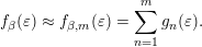 $$\begin{eqnarray}f_{\unicode[STIX]{x1D6FD}}(\unicode[STIX]{x1D700})\approx f_{\unicode[STIX]{x1D6FD},m}(\unicode[STIX]{x1D700})=\mathop{\sum }_{n=1}^{m}g_{n}(\unicode[STIX]{x1D700}).\end{eqnarray}$$
The corresponding matrix function approximation is
 $$\begin{eqnarray}f_{\unicode[STIX]{x1D6FD}}(H-\unicode[STIX]{x1D707})\approx f_{\unicode[STIX]{x1D6FD},m}(H-\unicode[STIX]{x1D707})=\mathop{\sum }_{n=1}^{m}g_{n}(H-\unicode[STIX]{x1D707}).\end{eqnarray}$$
The above formulation is general. We only require each term
 $g_{n}(H-\unicode[STIX]{x1D707})$
to be a simple function, so that the corresponding matrix function can be evaluated directly without diagonalizing the matrix. For instance,
 $g_{n}$
can be chosen to be a polynomial function or a rational function.
The approximation error of the matrix form (5.20) is directly related to that of the scalar form (5.19). Given the eigendecomposition
 $$\begin{eqnarray}H\unicode[STIX]{x1D713}_{i}=\unicode[STIX]{x1D700}_{i}\unicode[STIX]{x1D713}_{i},\end{eqnarray}$$
we have for any vector
 $v$
 $$\begin{eqnarray}(f_{\unicode[STIX]{x1D6FD}}(H-\unicode[STIX]{x1D707})-f_{\unicode[STIX]{x1D6FD},m}(H-\unicode[STIX]{x1D707}))v=\mathop{\sum }_{i}(f_{\unicode[STIX]{x1D6FD}}(\unicode[STIX]{x1D700}_{i}-\unicode[STIX]{x1D707})-f_{\unicode[STIX]{x1D6FD},m}(\unicode[STIX]{x1D700}_{i}-\unicode[STIX]{x1D707}))\unicode[STIX]{x1D713}_{i}\langle \unicode[STIX]{x1D713}_{i}|v\rangle .\end{eqnarray}$$
Thus,
 $$\begin{eqnarray}\displaystyle & & \displaystyle \Vert (f_{\unicode[STIX]{x1D6FD}}(H-\unicode[STIX]{x1D707})-f_{\unicode[STIX]{x1D6FD},m}(H-\unicode[STIX]{x1D707}))v\Vert _{2}^{2}\nonumber\\ \displaystyle & & \displaystyle \quad =\mathop{\sum }_{i}|f_{\unicode[STIX]{x1D6FD}}(\unicode[STIX]{x1D700}_{i}-\unicode[STIX]{x1D707})-f_{\unicode[STIX]{x1D6FD},m}(\unicode[STIX]{x1D700}_{i}-\unicode[STIX]{x1D707})|^{2}|\langle \unicode[STIX]{x1D713}_{i}|v\rangle |^{2}\nonumber\\ \displaystyle & & \displaystyle \quad \leq \sup _{i}|f_{\unicode[STIX]{x1D6FD}}(\unicode[STIX]{x1D700}_{i}-\unicode[STIX]{x1D707})-f_{\unicode[STIX]{x1D6FD},m}(\unicode[STIX]{x1D700}_{i}-\unicode[STIX]{x1D707})|^{2}\mathop{\sum }_{i}|\langle \unicode[STIX]{x1D713}_{i}|v\rangle |^{2}\nonumber\\ \displaystyle & & \displaystyle \quad =\sup _{t\in \operatorname{spec}(H-\unicode[STIX]{x1D707})}|f_{\unicode[STIX]{x1D6FD}}(t)-f_{\unicode[STIX]{x1D6FD},m}(t)|^{2}\Vert v\Vert _{2}^{2}.\end{eqnarray}$$
The equation above can be rewritten as
 $$\begin{eqnarray}\Vert f_{\unicode[STIX]{x1D6FD}}(H-\unicode[STIX]{x1D707})-f_{\unicode[STIX]{x1D6FD},m}(H-\unicode[STIX]{x1D707})\Vert _{2}\leq \Vert f_{\unicode[STIX]{x1D6FD}}(\cdot )-f_{\unicode[STIX]{x1D6FD},m}(\cdot )\Vert _{\infty },\end{eqnarray}$$
where the left-hand side is the operator norm for matrices and the right-hand side is the
 $L^{\infty }$
-norm for scalar functions. Thus the error of the Fermi operator expansion (5.20) will be small as long as the corresponding approximation is small in the sense of expansions for scalar functions (5.19).
One example of FOE is to expand the Fermi–Dirac function into polynomials (Goedecker and Colombo Reference Goedecker and Colombo1994):
 $$\begin{eqnarray}f_{\unicode[STIX]{x1D6FD}}(\unicode[STIX]{x1D700})\approx \mathop{\sum }_{n=1}^{m}c_{n}\unicode[STIX]{x1D700}^{n-1}.\end{eqnarray}$$
The corresponding matrix function version is
 $$\begin{eqnarray}f_{\unicode[STIX]{x1D6FD}}(H-\unicode[STIX]{x1D707})\approx \mathop{\sum }_{n=1}^{m}c_{n}(H-\unicode[STIX]{x1D707})^{n-1}.\end{eqnarray}$$
Note that each term of equation (5.25) is simply a matrix power
 $(H-\unicode[STIX]{x1D707})^{n}$
, which can be evaluated using only matrix–matrix multiplication recursively, without diagonalizing the matrix
 $H$
. In order to implement the FOE (5.25) for a high-order polynomial, it is more efficient and stable to expand
 $f_{\unicode[STIX]{x1D6FD}}(t)$
using Chebyshev polynomials. For insulators, the number of terms needed in equation (5.25) scales as
 $\log \unicode[STIX]{x1D716}^{-1}$
to reach target accuracy
 $\unicode[STIX]{x1D716}$
(Trefethen Reference Trefethen2008). In particular, the number of terms is independent of the system size and can be treated as a constant. When
 $H$
is a sparse matrix, this means that the polynomial approximation to
 $f_{\unicode[STIX]{x1D6FD}}(H-\unicode[STIX]{x1D707})$
is a sparse matrix as well, and the number of non-zeros only scales linearly with respect to the system size. Hence the FOE method (5.25) is a linear scaling algorithm.
Besides expansion using polynomials, another possibility is to approximate the Fermi–Dirac function using rational functions. A rational function can be decomposed into a linear combination of terms of the form
 $(\unicode[STIX]{x1D700}-z)^{-p}$
, where
 $z\in \mathbb{C}$
and
 $p\geq 1$
. In particular, if all terms use
 $p=1$
the resulting expansion is called a simple pole expansion, or just the pole expansion. Compared to polynomial expansion, there are two main advantages in using the rational expansion. First, the number of terms needed for the rational expansion can be much smaller than that needed for polynomial expansion to achieve the same accuracy. This is particularly the case for systems with small gaps. Second, the use of the pole expansion can yield fast algorithms with reduced complexity even for metallic systems. This is called the pole expansion and selected inversion algorithm (PEXSI), which will be discussed in Section 5.3. To our knowledge, PEXSI is so far the only algorithm allowing such complexity reduction.
5.3 Pole expansion and selected inversion method
While linear scaling algorithms in principle yield fast algorithms for the evaluation of Kohn–Sham maps, their accuracy often crucially depends on the decay of orbitals or density matrices, and they are usually only suitable for insulating systems with a large gap. Another practical drawback is that they often require user input on support of truncation and other tuning parameters to achieve a balance between efficiency and accuracy. The pole expansion and selected inversion method (PEXSI) (Lin et al.
Reference Lin, Lu, Ying, Car and E2009b
, Lin, Chen, Yang and He Reference Lin, Chen, Yang and He2013) is a reduced scaling algorithm with computational scaling at most
 $O(N^{2})$
and smaller for lower-dimensional systems. While it has a worse computational scaling than linear, the PEXSI algorithm can be applied to general systems and gives accurate results.
The PEXSI algorithm is one type of FOE method, and uses the following pole expansion to approximate the Fermi–Dirac distribution:
 $$\begin{eqnarray}P\approx \mathop{\sum }_{l=1}^{m}\unicode[STIX]{x1D714}_{l}(H-z_{l})^{-1}.\end{eqnarray}$$
If the band gap is small or zero, the number of terms needed in order for the polynomial expansion to reach a certain target accuracy
 $\unicode[STIX]{x1D716}$
scales as
 $O(\unicode[STIX]{x1D6FD}\unicode[STIX]{x1D6E5}E)$
, where
 $\unicode[STIX]{x1D6E5}E$
is the spectral radius of the shifted operator
 $H-\unicode[STIX]{x1D707}$
(Goedecker Reference Goedecker1999). Although the number of terms of a straightforward construction of the pole expansion also scales as
 $O(\unicode[STIX]{x1D6FD}\unicode[STIX]{x1D6E5}E)$
(Baroni and Giannozzi Reference Baroni and Giannozzi1992), it has subsequently been improved to
 $O((\unicode[STIX]{x1D6FD}\unicode[STIX]{x1D6E5}E)^{1/2})$
(Ozaki Reference Ozaki2007),
 $O((\unicode[STIX]{x1D6FD}\unicode[STIX]{x1D6E5}E)^{1/3})$
(Ceriotti, Kühne and Parrinello Reference Ceriotti, Kühne and Parrinello2008), and finally
 $O(\log (\unicode[STIX]{x1D6FD}\unicode[STIX]{x1D6E5}E))$
(Lin, Lu, Ying and E Reference Lin, Lu, Ying and E2009a
).
In order to obtain such a pole expansion, one possibility is to use the Cauchy contour integral formulation. Note that the Fermi–Dirac function
 $f_{\unicode[STIX]{x1D6FD}}(\unicode[STIX]{x1D700})=1/(1+\text{e}^{\unicode[STIX]{x1D6FD}\unicode[STIX]{x1D700}})$
is a meromorphic function in
 $\mathbb{C}$
, and the only poles are at
 $\unicode[STIX]{x1D700}=(2n+1)\text{i}\unicode[STIX]{x1D70B}/\unicode[STIX]{x1D6FD},n\in \mathbb{Z}$
. Furthermore,
 $f_{\unicode[STIX]{x1D6FD}}(\unicode[STIX]{x1D700})$
can be expanded using the following Matsubara expansion (Mahan Reference Mahan2000):
 $$\begin{eqnarray}f_{\unicode[STIX]{x1D6FD}}(\unicode[STIX]{x1D700})=\displaystyle \frac{1}{2}-\displaystyle \frac{1}{\unicode[STIX]{x1D6FD}}\mathop{\sum }_{n\in \mathbb{Z}}\displaystyle \frac{1}{\unicode[STIX]{x1D700}-(2n+1)\text{i}\unicode[STIX]{x1D70B}/\unicode[STIX]{x1D6FD}}.\end{eqnarray}$$
Note that equation (5.27) only converges conditionally, and the infinite summation must be performed symmetrically with respect to the positive and negative choices of
 $n$
. The number of terms needed in the direct truncation of the Matsubara series naturally scales as
 $O(\unicode[STIX]{x1D6FD}\unicode[STIX]{x1D6E5}E)$
.
The efficiency of the pole expansion can be improved by using a contour integral formulation:
 $$\begin{eqnarray}f_{\unicode[STIX]{x1D6FD}}(H-\unicode[STIX]{x1D707})=\displaystyle \frac{1}{2\unicode[STIX]{x1D70B}\text{i}}\oint _{\mathscr{C}}f_{\unicode[STIX]{x1D6FD}}(z)((z+\unicode[STIX]{x1D707})I-H)^{-1}\,\text{d}z.\end{eqnarray}$$
Here the contour
 $\mathscr{C}$
should be chosen so that it includes all the (real) eigenvalues of
 $H-\unicode[STIX]{x1D707}$
, without including any poles of
 $f_{\unicode[STIX]{x1D6FD}}(z)$
, i.e.
 $(2n+1)\text{i}\unicode[STIX]{x1D70B}/\unicode[STIX]{x1D6FD},n\in \mathbb{Z}$
. This leads to the ‘dumbbell-shaped’ contour used in Lin et al. (Reference Lin, Lu, Ying and E2009a
) (Figure 5.2). The contour is symmetric with respect to the chemical potential
 $\unicode[STIX]{x1D707}$
. The discretization points are chosen to be denser around
 $\unicode[STIX]{x1D707}$
to resolve the sharp transition of the Fermi–Dirac function at
 $\unicode[STIX]{x1D707}$
. At finite temperature, the contour integral formulation remains well-defined for gapless systems, i.e.
 $\unicode[STIX]{x1D700}_{N}=\unicode[STIX]{x1D700}_{N+1}$
.
Contour integral representation and pole expansion for the density matrix at finite temperature.
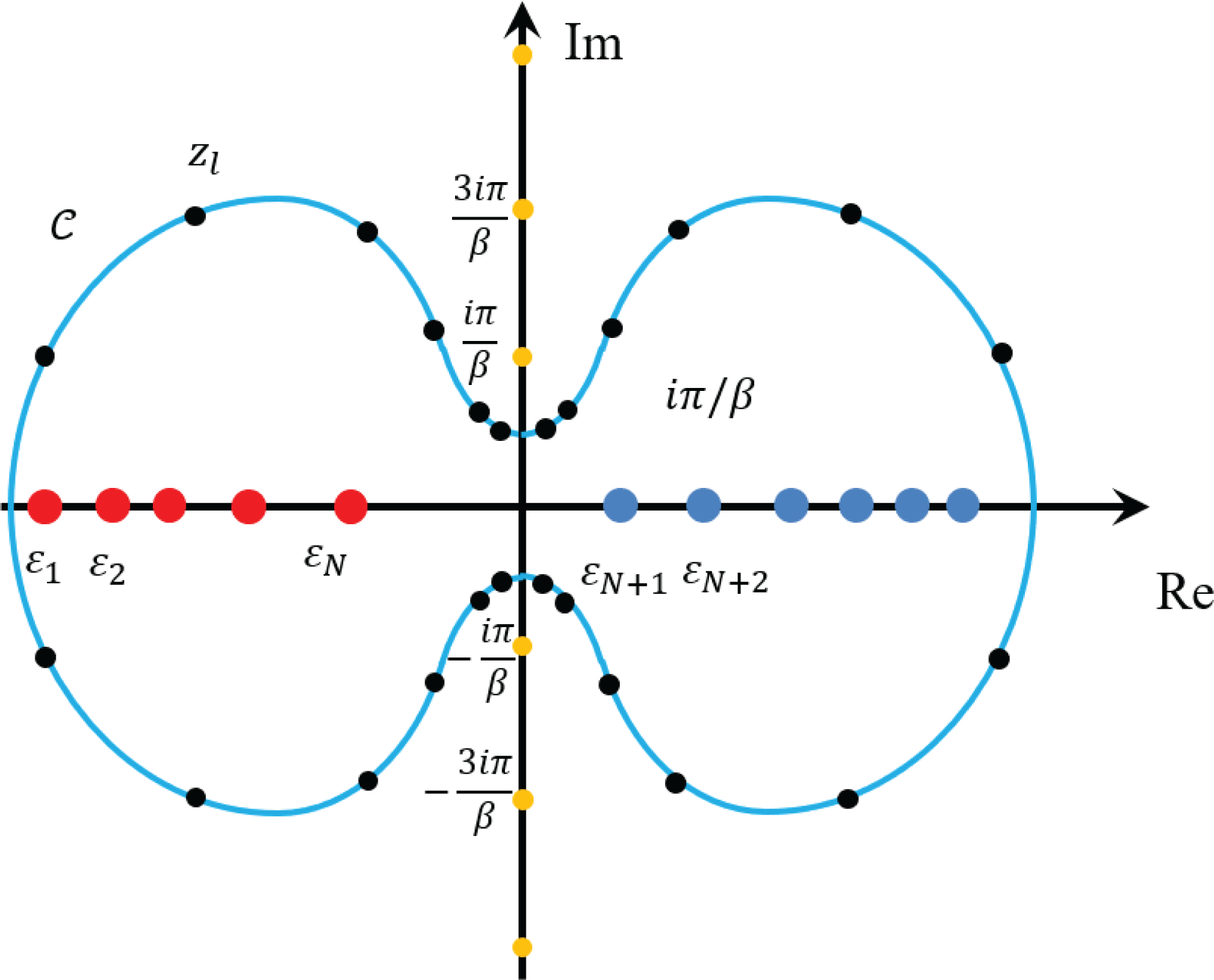
Each term in the pole expansion corresponds to a matrix inverse, or Green’s function
 $(z_{l}-H)^{-1}$
, which can be evaluated directly without diagonalizing the matrix
 $H$
. Equation (5.26) converts the problem of computing
 $P$
to the problem of computing
 $m$
Green’s functions. In order to find the Kohn–Sham map, we do not need the entire density matrix
 $P$
, but only the electron density which corresponds to the diagonal entries of
 $P$
(again for simplicity we assume that the basis set is orthogonal and the overlap matrix
 $S$
is an identity matrix). This amounts to the question of finding the diagonal entries of a Green’s function. Note that even if
 $H$
is a sparse matrix, the matrix inverse
 $G_{l}:=(z_{l}-H)^{-1}$
can be a fully dense matrix. One naive method is to first evaluate each Green’s function and extract its diagonal elements. However, when
 $H$
is a sparse matrix, the computation of diagonal entries, and more generally the entries of
 $G_{l}$
corresponding to the sparsity pattern of
 $H$
, can be evaluated much more efficiently by means of the selected inversion method (Erisman and Tinney Reference Erisman and Tinney1975, Lin et al.
Reference Lin, Lu, Ying, Car and E2009b
, Reference Lin, Yang, Meza, Lu, Ying and E2011, Jacquelin, Lin and Yang Reference Jacquelin, Lin and Yang2016).
Although we assume
 $H$
to be a general Hermitian matrix throughout the paper, for the simplicity of discussion in this section, we assume
 $H$
to be a real symmetric matrix. This makes
 $A=z_{l}-H\in \mathbb{C}^{N_{b}\times N_{b}}$
a complex symmetric, non-singular matrix. For such a matrix, the standard approach to computing
 $A^{-1}$
is to first decompose
 $A$
as
 $$\begin{eqnarray}A=LDL^{\top },\end{eqnarray}$$
where
 $L$
is a unit lower triangular matrix and
 $D$
is a diagonal or a block-diagonal matrix. Equation (5.29) is often known as the
 $LDL^{\top }$
factorization of
 $A$
. Given such a factorization, one can obtain
 $A^{-1}=(x_{1},x_{2},\ldots ,x_{N_{b}})$
by solving a number of triangular systems,
 $$\begin{eqnarray}Ly=e_{j},Dw=y,L^{\top }x_{j}=w,\end{eqnarray}$$
for
 $j=1,2,\ldots ,N_{b}$
, where
 $e_{j}$
is the
 $j$
th column of the identity matrix
 $I$
. The computational cost of such algorithms is generally
 $O(N_{b}^{3})$
. However, when
 $A$
is sparse, we can exploit the sparsity structure of
 $L$
and
 $e_{j}$
to reduce the complexity of computing selected components of
 $A^{-1}$
.
The selected inversion algorithm can be heuristically understood as follows (Lin et al.
Reference Lin, Yang, Meza, Lu, Ying and E2011). Let
 $A$
be partitioned into the
 $2\times 2$
block form
 $$\begin{eqnarray}A=\left(\begin{array}{@{}cc@{}}\unicode[STIX]{x1D6FC} & b^{\top }\\ b & \widetilde{A}\end{array}\right)\!.\end{eqnarray}$$
The first step of an
 $LDL^{\top }$
factorization produces a decomposition of
 $A$
that can be expressed by
 $$\begin{eqnarray}A=\left(\begin{array}{@{}cc@{}}1 & \\ \ell & I\end{array}\right)\left(\begin{array}{@{}cc@{}}\unicode[STIX]{x1D6FC} & \\ & \widetilde{A}-b\unicode[STIX]{x1D6FC}^{-1}b^{\top }\end{array}\right)\left(\begin{array}{@{}cc@{}}1 & \ell ^{\top }\\ & I\end{array}\right)\!,\end{eqnarray}$$
where
 $\unicode[STIX]{x1D6FC}$
is often referred to as a pivot,
 $\ell =b\unicode[STIX]{x1D6FC}^{-1}$
and
 $S=\widetilde{A}-b\unicode[STIX]{x1D6FC}^{-1}b^{\top }$
is known as the Schur complement. The same type of decomposition can be applied recursively to the Schur complement
 $S$
until its dimension becomes
 $1$
. The product of lower triangular matrices produced from the recursive procedure, which all have the form
 $$\begin{eqnarray}\left(\begin{array}{@{}ccc@{}}I & & \\ & 1 & \\ & \ell ^{(i)} & I\end{array}\right)\!,\end{eqnarray}$$
where
 $\ell ^{(1)}=\ell =b\unicode[STIX]{x1D6FC}^{-1}$
, yields the final
 $L$
factor. At this last step the matrix in the middle becomes diagonal, which is the
 $D$
matrix.
From equation (5.32),
 $A^{-1}$
can be expressed by
 $$\begin{eqnarray}A^{-1}=\left(\begin{array}{@{}cc@{}}\unicode[STIX]{x1D6FC}^{-1}+\ell ^{\top }S^{-1}\ell & -\ell ^{\top }S^{-1}\\ -S^{-1}\ell & S^{-1}\end{array}\right)\!.\end{eqnarray}$$
This expression suggests that once
 $\unicode[STIX]{x1D6FC}$
and
 $\ell$
are known, the task of computing
 $A^{-1}$
can be reduced to that of computing
 $S^{-1}$
. Because a sequence of Schur complements is produced recursively in the
 $LDL^{\top }$
factorization of
 $A$
, the computation of
 $A^{-1}$
can be organized in a recursive fashion too. Clearly, the reciprocal of the last entry of
 $D$
is the
 $(N_{b},N_{b})$
th entry of
 $A^{-1}$
. Starting from this entry, which is also the
 $1\times 1$
Schur complement produced in the
 $(N_{b}-1)$
th step of the
 $LDL^{\top }$
factorization procedure, we can construct the inverse of the
 $2\times 2$
Schur complement produced at the
 $(N_{b}-2)$
th step of the factorization procedure, using the recipe given by (5.33). This
 $2\times 2$
matrix is the trailing
 $2\times 2$
block of
 $A^{-1}$
. As we proceed from the lower right corner of
 $L$
and
 $D$
towards their upper left corner, more and more elements of
 $A^{-1}$
are recovered. Finally, we may recover all the diagonal entries of
 $A^{-1}$
exactly. In fact, given the factorization
 $A=LDL^{\top }$
, the selected inversion algorithm can be used to efficiently compute all entries
 $$\begin{eqnarray}\{A_{i,j}^{-1}\;:\;(L+L^{\top })_{i,j}\neq 0\}.\end{eqnarray}$$
The validity of the selected inversion algorithm can be verified by the following statement. For any
 $1\leq k<N_{b}$
, define
 $$\begin{eqnarray}\displaystyle {\mathcal{C}}=\{i\;:\;L_{i,k}\neq 0,i>k\}. & & \displaystyle\end{eqnarray}$$
Then all entries
 $\{A_{i,k}^{-1}\;:\;i\in {\mathcal{C}}\}$
,
 $\{A_{k,j}^{-1}\;:\;j\in {\mathcal{C}}\}$
, and
 $A_{k,k}^{-1}$
can be computed using only the
 $L,D$
factors and
 $$\begin{eqnarray}\{A_{i,j}^{-1}\;:\;(L+L^{\top })_{i,j}\neq 0,i,j>k\}.\end{eqnarray}$$
To see why this is the case, consider
 $\{A_{i,k}^{-1}\;:\;i\in {\mathcal{C}}\}$
. As in equation (5.33) we can derive
 $$\begin{eqnarray}A_{i,k}^{-1}=-\mathop{\sum }_{j=k+1}^{N_{b}}A_{i,j}^{-1}L_{j,k},\quad i\in {\mathcal{C}}.\end{eqnarray}$$
If
 $L_{j,k}\neq 0$
, then
 $A_{i,j}^{-1}$
is needed in the sum. Since we are only interested in computing
 $A_{i,k}^{-1}$
for
 $i\in {\mathcal{C}}$
, the
 $i$
and
 $j$
indices are constrained to satisfy the conditions
 $L_{j,k}\neq 0$
and
 $L_{i,k}\neq 0$
. Due to the non-zero fill-in pattern in the
 $LDL^{\top }$
factorization, we have
 $(L+L^{\top })_{i,j}\neq 0$
and the statement is proved for
 $\{A_{i,k}^{-1}\;:\;i\in {\mathcal{C}}\}$
. The argument is the same for
 $\{A_{k,j}^{-1}\;:\;j\in {\mathcal{C}}\}$
due to symmetry. Finally for the diagonal entry, we have
 $$\begin{eqnarray}A_{k,k}^{-1}=D_{k,k}^{-1}-\mathop{\sum }_{i=k+1}^{N_{b}}L_{i,k}A_{i,k}^{-1},\end{eqnarray}$$
which can be readily computed given
 $\{A_{i,k}^{-1}\;:\;i\in {\mathcal{C}}\}$
is available. This proves the statement above.

In order to understand the asymptotic complexity of the selected inversion algorithm, without loss of generality we assume the sparsity pattern of
 $H$
is similar to that obtained by the second-order central difference discretization of a Laplace operator. The computational cost associated with the
 $LDL^{\top }$
factorization, as well as the selected inversion algorithm, scales as
 $O(N_{b})$
,
 $O(N_{b}^{1.5})$
and
 $O(N_{b}^{2})$
for one-, two- and three-dimensional systems, respectively (Lin et al.
Reference Lin, Lu, Ying and E2009a
). We remark that such a complexity count is robust to changes of the discretization scheme as long as local basis sets are used. Hence for quasi-1D systems (such as nanotubes) and quasi-2D systems (such as monolayer systems and surfaces), the computational cost also scales as
 $O(N_{b})$
and
 $O(N_{b}^{1.5})$
, respectively. Pseudocode for the selected inversion algorithm is given in Algorithm 8.
In practice, a column-based sparse factorization and selected inversion algorithm as illustrated in Algorithm 8 may not be efficient due to the lack of level 3 BLAS operations. For a sparse matrix
 $A$
, the columns of
 $A$
and the
 $L$
factor can be partitioned into supernodes. A supernode is a set of contiguous columns
 ${\mathcal{J}}=\{j,j+1,\ldots ,j+s\}$
of the
 $L$
factor that have the same or similar non-zero sparsity structure below the
 $(j+s)$
th row (Ashcraft and Grimes Reference Ashcraft and Grimes1989). This allows use of matrix–matrix multiplications, which can significantly improve the efficiency.
The pole expansion and selected inversion (PEXSI) method (Lin et al.
Reference Lin, Lu, Ying and E2009a
, Reference Lin, Yang, Meza, Lu, Ying and E2011, Jacquelin et al.
Reference Jacquelin, Lin and Yang2016) therefore combines the pole expansion and the selected inversion, and evaluates the Kohn–Sham map without solving any eigenvalues or eigenfunctions. The selected inversion method is an exact method if exact arithmetic is used, that is, the only error in the selected inversion method is due to round-off errors. Hence the accuracy of the PEXSI method is determined by the pole expansion, which can be systematically improved by increasing the number of poles
 $m$
. The PEXSI method is ideally suited to massively parallel computers. The treatment of the poles can be parallelized in a straightforward fashion, with communication only needed at the end to construct the density matrix. The selected inversion method itself can also be massively parallelizable to thousands of processors (Jacquelin et al.
Reference Jacquelin, Lin and Yang2016), and the total number of processors that can be efficiently used by PEXSI can be over
 $100\,000$
.
The PEXSI software package (available at http://www.pexsi.org, distributed under the BSD license) has now been integrated into electronic structure packages such as BigDFT, CP2K, DGDFT, FHI-aims, QuantumWise ATK and SIESTA, and is part of the ‘Electronic Structure Infrastructure’ (ELSI) package (Yu et al. Reference Yu, Corsetti, García, Huhn, Jacquelin, Jia, Lange, Lin, Lu, Mi, Seifitokaldani, Vazquez-Mayagoitia, Yang, Yang and Blum2018).
In addition to computing the charge density at a reduced computational complexity in each SCF iteration, we can also use PEXSI to compute energy, free energy and the atomic forces efficiently without diagonalizing the Kohn–Sham Hamiltonian, using the same set of poles as those used for computing the charge density (Lin et al. Reference Lin, Chen, Yang and He2013). Another numerical issue associated with the PEXSI technique, as well as the Fermi operator expansion techniques in general, is to determine the chemical potential, so that the condition
 $$\begin{eqnarray}N=N_{\unicode[STIX]{x1D6FD}}(\unicode[STIX]{x1D707}):=\operatorname{Tr}[P]\end{eqnarray}$$
is satisfied. Note that
 $N_{\unicode[STIX]{x1D6FD}}(\cdot )$
is a non-decreasing function of
 $\unicode[STIX]{x1D707}$
. Hence the chemical potential can be determined via a bisection strategy, or Newton’s method. When Newton’s method is used, the chemical potential converges rapidly near its correct value. However, the standard Newton’s method may not be robust enough when the initial guess is far away from the correct chemical potential. It may give, for example, too large a correction when
 $N_{\unicode[STIX]{x1D6FD}}^{\prime }(\unicode[STIX]{x1D707})$
is close to zero, such as when
 $\unicode[STIX]{x1D707}$
is near the edge or in the middle of a band gap.
One way to overcome the above difficulty is to efficiently approximate the function
 $N_{\unicode[STIX]{x1D6FD}}(\unicode[STIX]{x1D700})$
to narrow down the region in which the correct
 $\unicode[STIX]{x1D707}$
must lie. This function can be seen effectively as a (temperature smeared) cumulative density of states, counting the number of eigenvalues in the interval
 $(-\infty ,\unicode[STIX]{x1D700})$
. We can evaluate such a zero temperature limit, denoted by
 $N_{\infty }(\unicode[STIX]{x1D700})$
, again without computing any eigenvalues of
 $H$
. Instead, we perform a matrix decomposition of the shifted matrix
 $H-\unicode[STIX]{x1D700}=LDL^{\top }$
, where
 $L$
is unit lower triangular and
 $D$
is diagonal. It follows from Sylvester’s law of inertia (Sylvester Reference Sylvester1852) that the inertia (the number of negative, zero and positive eigenvalues) of a real symmetric matrix does not change under a congruent transform, that
 $D$
has the same inertia as that of
 $H-\unicode[STIX]{x1D700}$
. Hence, we can obtain
 $N_{\infty }(\unicode[STIX]{x1D700})$
by simply counting the number of negative entries in
 $D$
. Note that the matrix decomposition
 $H-\unicode[STIX]{x1D700}=LDL^{\top }$
can be computed efficiently by using a sparse
 $LDL^{\top }$
or
 $LU$
factorization in real arithmetic. It requires fewer floating point operations than the complex arithmetic direct sparse factorization used in PEXSI.
We apply the parallel PEXSI method to the DG_Graphene_2048 and DG_Graphene_8192 systems, which are disordered graphene systems with
 $2048$
and
 $8192$
atoms, respectively, and compare its performance with a standard approach that requires a partial diagonalization of
 $(H,S)$
. We use a ScaLAPACK subroutine pdsyevr (Vömel Reference Vömel2010), which is based on the multiple relatively robust representations (MRRR) algorithm, to perform the diagonalization.
Figure 5.3 shows that for graphene problems with
 $2048$
and
 $8192$
processors, the PEXSI technique is nearly two orders of magnitude faster than the ScaLAPACK routine pdsyevr, and can be scalable to a much larger number of processors. The advantage of PEXSI becomes even clearer for a disordered graphene system with
 $32\,768$
atoms (see Figure 5.4). For this case, the diagonalization routine is no longer feasible, while the time to solution for the PEXSI technique can be as small as
 $241$
s.
(Credit: Jacquelin et al. Reference Jacquelin, Lin and Yang2016.) Wall clock time versus number of cores for a graphene system.
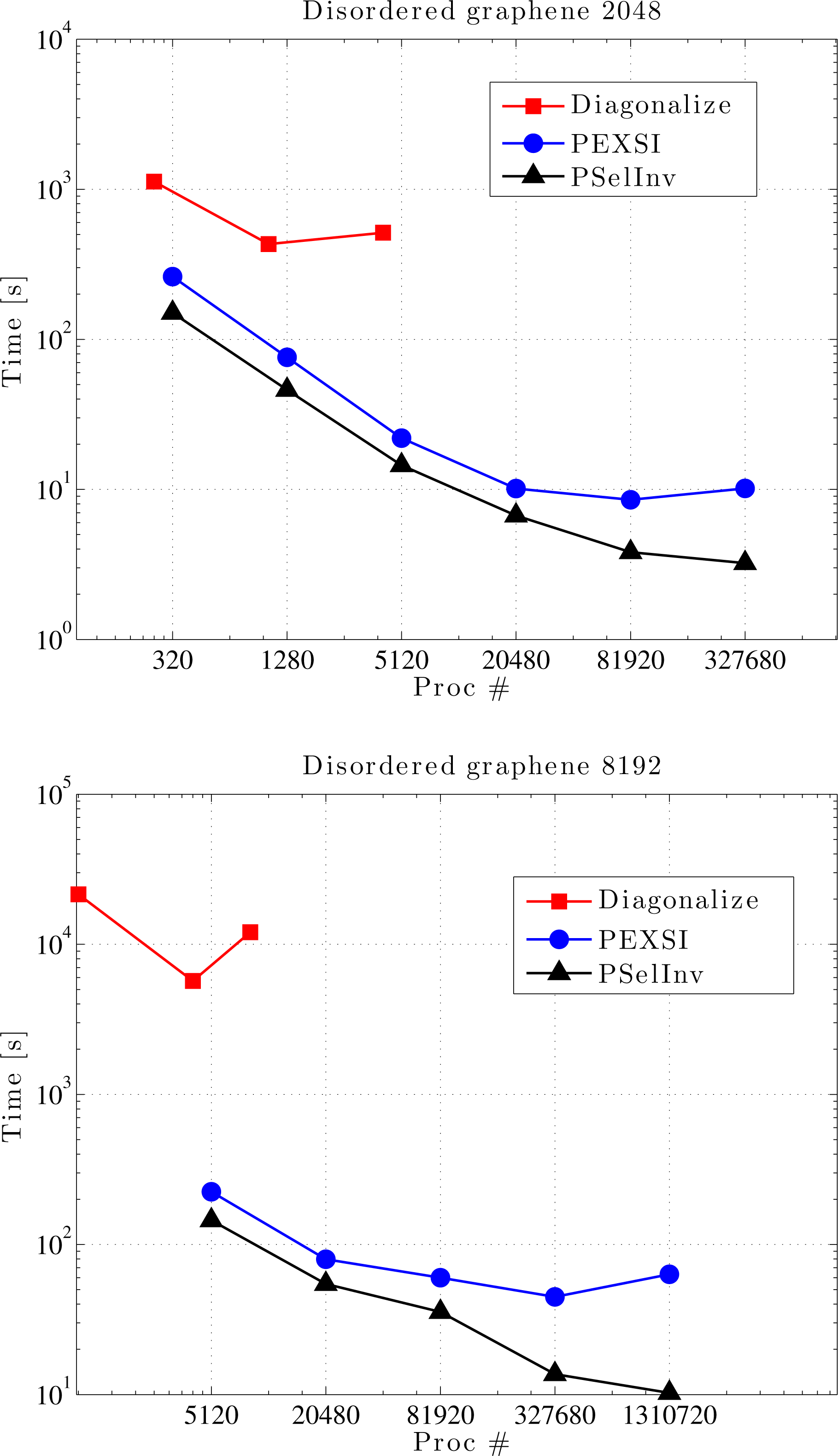
(Credit: Jacquelin et al.
Reference Jacquelin, Lin and Yang2016.) Wall clock time versus number of cores for a graphene system with
 $32\,768$
atoms.
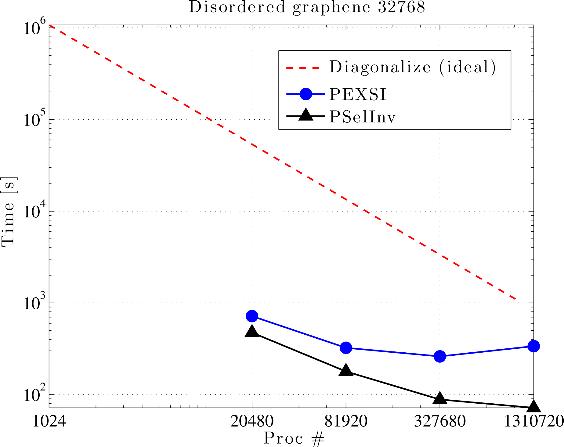
Remarks
Unlike most linear scaling algorithms discussed in this section, the PEXSI method does not rely on the decay properties of the density matrix. Hence the efficiency of PEXSI is roughly the same for metallic, semiconducting and insulating systems. For insulating systems with a relatively large energy gap, PEXSI may become slightly more efficient due to the potentially smaller number of poles needed to approximate the density matrix. The computational cost of PEXSI scales as
 $O(N_{b}^{\unicode[STIX]{x1D6FC}})$
, where
 $\unicode[STIX]{x1D6FC}=1,3/2,2$
for quasi-1D, 2D and 3D systems, respectively, where
 $N_{b}$
is the number of basis functions. Compared to dense eigensolvers which scale as
 $O(N_{b}^{3})$
, the PEXSI method can be highly advantageous for large systems, as demonstrated in numerical results above. On the other hand, recall that iterative diagonalization methods discussed in Section 4.2 scale as
 $O(N_{b}N^{2})$
; we find that the cross-over point between PEXSI and iterative diagonalization methods is roughly at
 $N\sim N_{b}^{(\unicode[STIX]{x1D6FC}-1)/2}$
. This implies that PEXSI is most efficient when small basis sets such as Gaussian-type orbitals are used, and becomes less efficient for large basis sets such as finite elements. This statement is in fact true for most linear scaling methods discussed in Section 5.2.
In the discussion above, we have assumed that
 $H$
is a real symmetric matrix, and hence
 $A=z_{l}-H$
is complex symmetric. This assumption is valid for molecular systems, as well as
 $\unicode[STIX]{x1D6E4}$
point sampling of periodic systems. In a more general situation, such as in the context of
 $\mathbf{k}$
-point sampling for periodic systems, or when the system is magnetic,
 $H$
is a Hermitian matrix, and
 $A=z_{l}-H$
is merely a structurally symmetric matrix. In such a case, the
 $LDL^{\top }$
factorization should be replaced by the
 $LU$
factorization, and the non-symmetric version of the selected inversion algorithm should be used instead (Jacquelin, Lin and Yang Reference Jacquelin, Lin and Yang2018). Besides PEXSI, general-purpose selected inversion algorithms are also available in other software packages such as PARDISO (Schenk and Gartner Reference Schenk and Gartner2006) and MUMPS (Amestoy, Duff, L’Excellent and Koster Reference Amestoy, Duff, L’Excellent and Koster2001). The selected inversion-type algorithms are also used in other contexts such as quantum transport calculations (Li, Ahmed, Klimeck and Darve Reference Li, Ahmed, Klimeck and Darve2008, Petersen et al.
Reference Petersen, Li, Stokbro, Sørensen, Hansen, Skelboe and Darve2009).
Recently it has been shown that the pre-constant of the logarithmic scaling factor can be further reduced to be numerically near-optimal (Moussa Reference Moussa2016). This makes the pole expansion highly efficient for metallic systems, and the number of poles needed in practical calculations is typically only
 $10\sim 40$
.
During the self-consistency field iteration, the zero temperature limit
 $N_{\infty }(\unicode[STIX]{x1D700})$
evaluated from the inertia-counting procedure may be used to construct upper and lower bounds on the chemical potential. Then, coupled with a strategy to evaluate
 $N_{\unicode[STIX]{x1D6FD}}(\unicode[STIX]{x1D700})$
accurately using PEXSI over multiple energy points
 $\unicode[STIX]{x1D700}$
, we may accurately determine the chemical potential within the window specified by the inertia-counting procedure. In particular, it is possible to perform PEXSI calculations over multiple energy points only once per SCF iteration, without sacrificing accuracy at convergence (Jia and Lin Reference Jia and Lin2017).
6 Evaluation of the Kohn–Sham map: non-local functional
Kohn–Sham DFT calculations with non-local functionals, such as rung-
 $4$
functionals (hybrid functionals) and rung-
 $5$
functionals, can be considerably more costly than calculations with exchange-correlation functionals from the first three rungs of the ladder. More specifically, Kohn–Sham equations with local and semi-local functionals can be viewed as eigenvalue problems corresponding to differential operators. When a rung-
 $4$
functional is used, the Kohn–Sham Hamiltonian operator becomes an integro-differential operator due to the Fock exchange term. For rung-
 $5$
functionals, the self-consistency is computationally rather challenging, and most calculations are done as a post-processing step to obtain the correlation energy as a perturbation to the self-consistent solution for a semi-local functional.
Throughout the discussion in this section, we assume that a large basis set such as planewaves or real-space representation is used. We first discuss numerical methods for evaluating the Fock exchange operator in Section 6.1. We introduce an acceleration technique called the adaptive compression method in Section 6.2. We discuss a method for evaluating the RPA correlation energy as an example of the rung-
 $5$
functionals in Section 6.3.
6.1 Fock exchange operator
The Fock exchange operator
 $V_{\text{x}}^{\text{EX}}[P]$
is an integral operator, introduced in equation (2.52), recalled here for readers’ convenience:
 $$\begin{eqnarray}V_{\text{x}}^{\text{EX}}[P](\mathbf{r},\mathbf{r}^{\prime })=-P(\mathbf{r},\mathbf{r}^{\prime })K(\mathbf{r},\mathbf{r}^{\prime }),\end{eqnarray}$$
where
 $$\begin{eqnarray}P(\mathbf{r},\mathbf{r}^{\prime })=\mathop{\sum }_{i=1}^{N}\unicode[STIX]{x1D713}_{i}(\mathbf{r})\unicode[STIX]{x1D713}_{i}^{\ast }(\mathbf{r}^{\prime }).\end{eqnarray}$$
Here we assume the system is an insulating system for simplicity. The kernel of
 $V_{\text{x}}^{\text{EX}}[P]$
is not of low rank due to the Hadamard product (i.e. element-wise product) between the kernels of
 $P$
and
 $K$
. When a small basis set
 $\unicode[STIX]{x1D6F7}=[\unicode[STIX]{x1D719}_{1},\ldots ,\unicode[STIX]{x1D719}_{N_{b}}]$
is used, each occupied orbital is expanded as
 $$\begin{eqnarray}\unicode[STIX]{x1D713}_{i}(\mathbf{r})=\mathop{\sum }_{p}\unicode[STIX]{x1D719}_{p}(\mathbf{r})c_{p,i},\quad i=1,\ldots ,N.\end{eqnarray}$$
The matrix elements of the Fock exchange operator become
 $$\begin{eqnarray}\displaystyle (V_{\text{x}}^{\text{EX}}[P])_{pq} & = & \displaystyle -\int \unicode[STIX]{x1D719}_{p}^{\ast }(\mathbf{r})P(\mathbf{r},\mathbf{r}^{\prime })K(\mathbf{r},\mathbf{r}^{\prime })\unicode[STIX]{x1D719}_{q}(\mathbf{r}^{\prime })\,\text{d}\mathbf{r}\,\text{d}\mathbf{r}^{\prime }\nonumber\\ \displaystyle & = & \displaystyle -\mathop{\sum }_{i=1}^{N}\mathop{\sum }_{r,s}c_{r,i}c_{s,i}^{\ast }\int \unicode[STIX]{x1D719}_{p}^{\ast }(\mathbf{r})\unicode[STIX]{x1D719}_{r}(\mathbf{r})\unicode[STIX]{x1D719}_{s}^{\ast }(\mathbf{r}^{\prime })\unicode[STIX]{x1D719}_{q}(\mathbf{r}^{\prime })K(\mathbf{r},\mathbf{r}^{\prime })\,\text{d}\mathbf{r}\,\text{d}\mathbf{r}^{\prime }\nonumber\\ \displaystyle & := & \displaystyle -\mathop{\sum }_{i=1}^{N}\mathop{\sum }_{r,s}c_{r,i}c_{s,i}^{\ast }\langle ps|rq\rangle .\end{eqnarray}$$
Equation (6.2) defines the two-electron integral tensor
 $\langle ps|rq\rangle$
, which is a fourth-order tensor. Hence the computational cost of constructing the Fock exchange matrix
 $(V_{\text{x}}^{\text{EX}}[P])_{pq}$
typically scales as
 $O(N^{4})$
.
It turns out that when a large basis set is used, the asymptotic complexity associated with the Fock exchange operator can be reduced to
 $O(N^{3})$
without approximation. Note that in such a case, it is often prohibitively expensive to explicitly construct or to store the Fock exchange operator directly. It is only viable to apply it to an occupied orbital
 $\unicode[STIX]{x1D713}_{j}$
as
 $$\begin{eqnarray}(V_{\text{x}}^{\text{EX}}[P]\unicode[STIX]{x1D713}_{j})(\mathbf{r})=-\mathop{\sum }_{i=1}^{N}\unicode[STIX]{x1D711}_{i}(\mathbf{r})\int K(\mathbf{r},\mathbf{r}^{\prime })\unicode[STIX]{x1D711}_{i}^{\ast }(\mathbf{r}^{\prime })\unicode[STIX]{x1D713}_{j}(\mathbf{r}^{\prime })\,\text{d}\mathbf{r}^{\prime },\end{eqnarray}$$
for
 $$\begin{eqnarray}P=\mathop{\sum }_{i=1}^{N}|\unicode[STIX]{x1D711}_{i}\rangle \langle \unicode[STIX]{x1D711}_{i}|.\end{eqnarray}$$
Here we deliberately distinguish the orbitals in the density matrix (
 $\{\unicode[STIX]{x1D711}_{i}\}$
) and the orbitals
 $V_{\text{x}}^{\text{EX}}$
acts on (
 $\{\unicode[STIX]{x1D713}_{j}\}$
) to emphasize that they may correspond to different density matrices before self-consistency is achieved. The integral
 $\int K(\mathbf{r},\mathbf{r}^{\prime })\unicode[STIX]{x1D711}_{i}^{\ast }(\mathbf{r}^{\prime })\unicode[STIX]{x1D713}(\mathbf{r}^{\prime })\,\text{d}\mathbf{r}^{\prime }$
can be implemented by solving
 $N$
Poisson-like equations. Let
 $N_{g}$
denote the grid size, and the computational cost of solving each Poisson-like equation scales as
 $O(N_{g}\log N_{g})$
when fast Fourier transform can be used. When applied to all pairs of occupied orbitals, the computational cost scales as
 $O(N_{g}\log N_{g}N^{2})$
to
 $O(N^{3})$
. Note that the preconstant of this cubic scaling component can be very large. In practical Hartree–Fock calculations, the application of the Fock exchange operator can often take more than
 $95\%$
of the overall computational time.
The Hartree–Fock-like equations require the density matrix
 $P$
to be computed self-consistently. A common strategy is to solve the linearized Hartree–Fock equation by fixing the density matrix
 $P$
so that
 $H[P]$
becomes a fixed operator. Then one solves a nonlinear fixed-point problem to obtain the self-consistent
 $P$
. The most time-consuming step is to solve the linearized Hartree–Fock equation. We will describe the strategy for achieving self-consistency in Section 7.4.
In order to reduce the computational cost of evaluating the Fock exchange operator, one strategy is to compute in parallel with a large number of cores. Note that the
 $N^{2}$
Poisson-like equations associated with the pair products
 $\unicode[STIX]{x1D711}_{i}^{\ast }(\mathbf{r})\unicode[STIX]{x1D713}_{j}(\mathbf{r})$
are independent of each other. Hence one may employ in principle
 $O(N^{2})$
processors to distribute the work (Duchemin and Gygi Reference Duchemin and Gygi2010, Valiev et al.
Reference Valiev, Bylaska, Govind, Kowalski, Straatsma, Van Dam, Wang, Nieplocha, Apra, Windus and De Jong2010). The disadvantage of this approach is that the rest of the components of a Kohn–Sham solver often cannot scale to such a large number of processors, and hence the excessive number of computational cores may not be used efficiently.
In Section 4.3, we have introduced localization techniques to find localized representations of the Kohn–Sham subspace via the density matrix and Wannier functions. These techniques can be used to reduce the computational cost of evaluating the Kohn–Sham map as in Section 5. They can also be used to reduce the cost of applying exchange operators to
 $O(N)$
. More specifically, let
 $\{\unicode[STIX]{x1D711}_{i}\},\{\unicode[STIX]{x1D713}_{j}\}$
be exponentially localized Wannier functions after a proper rotation operation, and the pair product
 $\unicode[STIX]{x1D711}_{i}^{\ast }(\mathbf{r})\unicode[STIX]{x1D713}_{j}(\mathbf{r})$
would vanish if the support sets of
 $\unicode[STIX]{x1D711}_{i}$
and
 $\unicode[STIX]{x1D713}_{j}$
do not overlap with each other. This reduces the number of pairs from
 $O(N^{2})$
to
 $O(N)$
. Furthermore, each Poisson-like equation only needs to be solved on a computational domain that is independent of the system size. Taking both factors into account, we find that the cost of equation (6.3) is reduced to
 $O(N)$
. We refer readers to Wu, Selloni and Car (Reference Wu, Selloni and Car2009) and Dawson and Gygi (Reference Dawson and Gygi2015), for example, for more details of linear scaling hybrid functional calculations. As in the discussion in Section 5.2, linear scaling algorithms typically have a large prefactor, and hence they become advantageous to the cubic scaling methods only for systems of relatively large sizes.
On the other hand, for metallic and semi-conducting systems, the decay rate of the density matrix along the off-diagonal direction can be very slow. This may also introduce a significantly larger number of non-zero entries in the Hamiltonian matrix. Hence Green’s function-based methods, such as the PEXSI method, become less efficient in the context of hybrid functional calculations.
However, the interpolative separable density fitting (ISDF) (Lu and Ying Reference Lu and Ying2015) technique introduced in Section 4.4 can be applicable to insulating, semiconducting and metallic systems. Following the ISDF decomposition equation (4.13), the Poisson-like equation only needs to be solved with
 $\{\unicode[STIX]{x1D701}_{\unicode[STIX]{x1D707}}(\mathbf{r})\}$
on the right-hand side. This reduces the number of Poisson-like equations from
 $O(N^{2})$
to
 $N_{\unicode[STIX]{x1D707}}\sim O(N)$
. Of course, the solutions of these equations need to be reassembled through linear algebra operations to obtain
 $\{V_{\text{x}}^{\text{EX}}[P]\unicode[STIX]{x1D713}_{j}\}_{j=1}^{N}$
. The cost of these linear algebra steps is still
 $O(N^{3})$
but the preconstant can be effectively reduced (Hu et al.
Reference Hu, Lin and Yang2017a
, Dong et al.
Reference Dong, Hu and Lin2018). Hence ISDF is effective when it is relatively costly to solve Poisson-like equations, such as in the context of planewave methods, and even more so for finite difference and finite element methods.
6.2 Adaptive compression method
When a large basis set is used, the standard method for solving Hartree–Fock-like equations self-consistently is the two-level nested SCF method in Section 7.4. The motivation for this method is that the Fock exchange energy is only a small fraction (usually
 $5\%$
or less) of the total energy, although such a contribution is sufficient to result in qualitatively different results for the study of many chemical systems. The main idea is then to separate the self-consistent field (SCF) iteration into two sets of SCF iterations. In the inner SCF iteration, the exchange operation
 $V_{\text{x}}^{\text{EX}}$
defined by a set of orbitals
 $\{\unicode[STIX]{x1D711}_{i}\}_{i=1}^{N}$
is fixed, and the Hamiltonian operator depends only on the density
 $\unicode[STIX]{x1D70C}(\mathbf{r})$
. This allows the use of efficient charge mixing schemes to reduce the number of SCF iterations. In other words, the SCF iteration then proceeds as in Kohn–Sham DFT calculations with a fixed exchange operator. In the outer SCF iteration, the orbitals defining the exchange operator are updated via a fixed-point iteration. Furthermore, each inner SCF iteration requires the solution of a linear eigenvalue problem, which is to be performed with iterative diagonalization methods discussed in Section 4.2 and requires repeated application of the Hamiltonian operator to occupied orbitals. The application of the Fock exchange operator to occupied orbitals according to equation (6.3) appears in this innermost loop, which makes electronic structure calculations with rung-4 functionals much more costly than those with rung-1 to rung-3 functionals.
The adaptively compressed exchange operator (ACE) method (Lin Reference Lin2016) accelerates hybrid functional calculations by reducing the frequency of applications of the Fock exchange operator without compromising the accuracy of the self-consistent solution. This is achieved by constructing a low-rank surrogate operator, denoted by
 $\widetilde{V}_{\text{x}}^{\text{EX}}$
, to approximate the Fock exchange operator
 $V_{\text{x}}^{\text{EX}}$
. Note that
 $V_{\text{x}}^{\text{EX}}$
is generally a dense, full-rank operator. Hence the low-rank surrogate cannot be expected to be accurate when applied to an arbitrary vector. Instead we only require
 $\widetilde{V}_{\text{x}}^{\text{EX}}$
to be accurate when applied to all occupied orbitals.
More specifically, for a given set of orbitals
 $\{\unicode[STIX]{x1D711}_{i}\}_{i=1}^{N}$
defining the density matrix implicitly and thus the exchange operator, we first compute the application of the exchange operator to
 $\{\unicode[STIX]{x1D711}_{i}\}_{i=1}^{N}$
using
 $$\begin{eqnarray}W_{i}(\mathbf{r})=(V_{\text{x}}^{\text{EX}}[\{\unicode[STIX]{x1D711}\}]\unicode[STIX]{x1D711}_{i})(\mathbf{r}),\quad i=1,\ldots ,N.\end{eqnarray}$$
The adaptively compressed exchange operator, denoted by
 $\widetilde{V}_{\text{x}}^{\text{EX}}$
, should satisfy the conditions
 $$\begin{eqnarray}(\widetilde{V}_{\text{x}}^{\text{EX}}\unicode[STIX]{x1D711}_{i})(\mathbf{r})=W_{i}(\mathbf{r})\quad \text{and}\quad \widetilde{V}_{\text{x}}^{\text{EX}}(\mathbf{r},\mathbf{r}^{\prime })=(\widetilde{V}_{\text{x}}^{\text{EX}}(\mathbf{r}^{\prime },\mathbf{r}))^{\ast }.\end{eqnarray}$$
The choice of this surrogate operator is not unique. One possible choice satisfying the conditions (6.5) is given by
 $$\begin{eqnarray}\widetilde{V}_{\text{x}}^{\text{EX}}(\mathbf{r},\mathbf{r}^{\prime })=\mathop{\sum }_{i,j=1}^{N}W_{i}(\mathbf{r})B_{ij}W_{j}^{\ast }(\mathbf{r}^{\prime }),\end{eqnarray}$$
where
 $B=M^{-1}$
is a negative definite matrix, and
 $$\begin{eqnarray}M_{kl}=\int \unicode[STIX]{x1D711}_{k}^{\ast }(\mathbf{r})W_{l}(\mathbf{r})\,\text{d}\mathbf{r}.\end{eqnarray}$$
Perform Cholesky factorization for
 $-M$
, i.e.
 $M=-LL^{\ast }$
, where
 $L$
is a lower triangular matrix. Then we get
 $B=-L^{-\ast }L^{-1}$
. Define the projection vector in the ACE formulation as
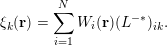 $$\begin{eqnarray}\unicode[STIX]{x1D709}_{k}(\mathbf{r})=\mathop{\sum }_{i=1}^{N}W_{i}(\mathbf{r})(L^{-\ast })_{ik}.\end{eqnarray}$$
Then the adaptively compressed exchange operator is given by
 $$\begin{eqnarray}\widetilde{V}_{\text{x}}^{\text{EX}}(\mathbf{r},\mathbf{r}^{\prime })=-\mathop{\sum }_{k=1}^{N}\unicode[STIX]{x1D709}_{k}(\mathbf{r})\unicode[STIX]{x1D709}_{k}(\mathbf{r}^{\prime }).\end{eqnarray}$$
The ACE can be readily used to reduce the computational cost of the exchange energy, without the need to solve any extra Poisson equations, using
 $$\begin{eqnarray}\displaystyle E_{\text{x}}^{\text{EX}} & = & \displaystyle \displaystyle \frac{1}{2}\mathop{\sum }_{i=1}^{N}\iint \unicode[STIX]{x1D713}_{i}^{\ast }(\mathbf{r})\widetilde{V}_{\text{x}}^{\text{EX}}(\mathbf{r},\mathbf{r}^{\prime })\unicode[STIX]{x1D713}_{i}(\mathbf{r}^{\prime })\,\text{d}\mathbf{r}\,\text{d}\mathbf{r}^{\prime }\nonumber\\ \displaystyle & = & \displaystyle -\displaystyle \frac{1}{2}\mathop{\sum }_{i,k=1}^{N}\biggl|\int \unicode[STIX]{x1D713}_{i}^{\ast }(\mathbf{r})\unicode[STIX]{x1D709}_{k}(\mathbf{r})\,\text{d}\mathbf{r}\biggr|^{2}.\end{eqnarray}$$
Note that once ACE is constructed, the cost of applying
 $\widetilde{V}_{\text{x}}^{\text{EX}}$
to any orbital
 $\unicode[STIX]{x1D713}$
is similar to the application of a non-local pseudopotential operator, thanks to its low-rank structure. ACE only needs to be constructed once per outer iteration, and can be repeatedly used for all the subsequent inner SCF iterations for the electron density, and each iterative step for solving the linear eigenvalue problem. The ACE formulation has been integrated in electronic structure software packages such as Quantum ESPRESSO.
Table 6.1 demonstrates the accuracy of the ACE formulation for Kohn–Sham DFT calculations with the HSE06 (Heyd et al.
Reference Heyd, Scuseria and Ernzerhof2003) hybrid functional, for silicon systems ranging from
 $64$
to
 $1000$
atoms. The ACE formulation can evaluate the HF energy and energy gap accurately (total energy difference is under
 $10^{-4}$
Hartree) even for large systems, and the remaining difference is in fact due to the tolerance of the SCF iteration. Table 6.2 demonstrates that ACE can perform hybrid functional calculations at a fraction of the cost of conventional methods (Hu et al.
Reference Hu, Lin, Banerjee, Vecharynski and Yang2017c
).
Comparison between the conventional hybrid DFT calculations and ACE-enabled hybrid DFT calculations in terms of the HF energy
 $E_{\text{x}}^{\text{EX}}$
(Hartree) and the energy gap
 $E_{\text{gap}}$
(Hartree) for the Si
 $_{64}$
, Si
 $_{216}$
, Si
 $_{512}$
and Si
 $_{1000}$
systems. The corresponding relative errors of the HF energy are shown in parentheses.
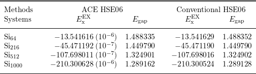
Comparison between the conventional hybrid DFT calculation and an ACE-enabled hybrid DFT calculation in terms of the number of inner SCF iterations and wall clock time spent in each outer SCF iteration for Si
 $_{1000}$
on 2000 cores.
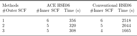
The efficiency of the ACE formulation also rests on the assumption that the magnitude of the Fock exchange operator is relatively small compared to other components of the Hamiltonian. To be more specific, we demonstrate below that in the context of linearized Hartree–Fock-like equations, the ACE formulation leads to desirable convergence properties compared to standard iterative solvers.
To make the discussion more general, we consider the following linear eigenvalue problem (linearized Hartree–Fock-like equations take this form):
 $$\begin{eqnarray}(A+B)v_{i}=\unicode[STIX]{x1D706}_{i}v_{i},\quad i=1,\ldots ,N.\end{eqnarray}$$
Here
 $A,B\in \mathbb{C}^{N_{b}\times N_{b}}$
are Hermitian matrices. The eigenvalues
 $\{\unicode[STIX]{x1D706}_{i}\}$
are real and ordered non-decreasingly. Due to the Pauli exclusion principle we need to compute the eigenpairs
 $(\unicode[STIX]{x1D706}_{i},v_{i})$
corresponding to the lowest
 $N$
eigenvalues, which are assumed to be separated from the rest of the eigenvalues by a positive spectral gap
 $\unicode[STIX]{x1D706}_{g}:=\unicode[STIX]{x1D706}_{N+1}-\unicode[STIX]{x1D706}_{N}$
. The matrix
 $A$
in (6.10) is obtained by discretizing the Hamiltonian operator excluding the exchange operator, while
 $B$
as a discretization of the exchange operator is negative definite.
In order to reduce the number of matrix–vector multiplication operations
 $Bv$
, the simplest idea is to fix
 $w_{i}:=Bv_{i}$
at some stage, and to replace
 $Bv_{i}$
with
 $w_{i}$
for a number of iterations. This leads to the following subproblem:
 $$\begin{eqnarray}Av_{i}+w_{i}=\unicode[STIX]{x1D706}_{i}v_{i},\quad i=1,\ldots ,N.\end{eqnarray}$$
Note that equation (6.11) is not an eigenvalue problem: if
 $v_{i}$
is a solution to (6.11), then
 $v_{i}$
multiplied by a constant
 $c$
is typically not a solution. Equation (6.11) could be solved using optimization-based methods, but such a problem is typically more difficult than a Hermitian eigenvalue problem. In practice, software packages for solving Hartree–Fock-like equations are typically built around eigensolvers, which is another important factor that makes subproblem (6.11) undesirable.
The adaptive compression method re-uses the information in
 $\{w_{i}\}$
in a different way, retaining the structure of the eigenvalue problem (6.10). Define
 $V=[v_{1},\ldots ,v_{N}]$
,
 $W=[w_{1},\ldots ,w_{N}]$
, so
 $V,W\in \mathbb{C}^{N_{b}\times N}$
, and construct
 $$\begin{eqnarray}\widetilde{B}[V]=W(W^{\ast }V)^{-1}W^{\ast }.\end{eqnarray}$$
Since
 $B\prec 0$
,
 $W^{\ast }V\equiv V^{\ast }BV$
has only negative eigenvalues and is invertible.
 $\widetilde{B}[V]$
is Hermitian of rank
 $N$
, and agrees with
 $B$
when applied to
 $V$
as
 $$\begin{eqnarray}\widetilde{B}[V]V=W(W^{\ast }V)^{-1}W^{\ast }V=W=BV.\end{eqnarray}$$
We shall refer to the operation from
 $B$
to
 $\widetilde{B}[V]$
as an adaptive compression. It turns out that the adaptive compression
 $\widetilde{B}[V]$
is the unique rank-
 $N$
Hermitian matrix that agrees with
 $B$
on
 $\operatorname{span}~V$
. Furthermore,
 $B\preccurlyeq \widetilde{B}[V]\preccurlyeq 0$
(Lin and Lindsey Reference Lin and Lindsey2019).
Note that the subspace
 $\text{span}V$
is precisely the solution for (6.10) and is not known a priori. Therefore
 $\widetilde{B}$
needs to be constructed in an adaptive manner. Starting from some initial guess
 $V^{(0)}$
, we will obtain a sequence
 $V^{(k)}$
and corresponding compressed operators
 $\widetilde{B}[V^{(k)}]$
. More specifically, ACE uses a fixed-point iteration given by
 $$\begin{eqnarray}(A+\widetilde{B}[V^{(k)}])v_{i}^{(k+1)}=\unicode[STIX]{x1D706}_{i}^{(k+1)}v_{i}^{(k+1)},\quad i=1,\ldots ,N.\end{eqnarray}$$
In each iteration, after
 $\widetilde{B}[V^{(k)}]$
is constructed, (6.14) can be solved via any iterative eigensolver to obtain
 $V^{(k+1)}$
. The iterative eigensolver only requires application of
 $A$
and the low-rank matrix
 $\widetilde{B}$
to vectors, and does not require any additional application of
 $B$
until
 $V^{(k+1)}$
is obtained. If
 $\text{span }V^{(k)}$
converges to
 $\text{span }V$
, then the consistency condition
 $\widetilde{B}[V]V=BV$
is satisfied, and the adaptive compression method is numerically exact. The adaptive compression method for solving the linear eigenvalue problem (6.10) is given in Algorithm 9, where we initialize
 $V^{(0)}$
by solving the eigenvalue problem in the absence of
 $B$
.

At first glance, the advantage of converting a linear eigenvalue problem (6.10) into a nonlinear eigenvalue problem (6.14) is unclear. The advantage of the adaptive compression method comes from the decoupling of the matrix–vector multiplication operations
 $Av$
and
 $Bv$
, and asymptotically the number of
 $Bv$
operations is independent of the spectral radius
 $\Vert A\Vert _{2}$
. More specifically, starting from an initial density matrix
 $P^{(0)}$
, the asymptotic convergence rate measured by the convergence of the density matrix at the
 $k$
th iteration is given by
 $$\begin{eqnarray}\Vert P-P^{(k)}\Vert _{2}\lesssim \unicode[STIX]{x1D6FE}^{k}\Vert P-P^{(0)}\Vert _{2},\quad \text{where}~\unicode[STIX]{x1D6FE}\leq \displaystyle \frac{\Vert B\Vert _{2}}{\Vert B\Vert _{2}+\unicode[STIX]{x1D706}_{g}}.\end{eqnarray}$$
Furthermore, one may prove that the adaptive compression method converges globally starting from almost every initial guess. We refer readers to Lin and Lindsey (Reference Lin and Lindsey2019) for more details.
Remarks
An alternative way to adaptively reduce the rank of the exchange operator is via a projector-based compression of the exchange operator (Duchemin and Gygi Reference Duchemin and Gygi2010, Boffi, Jain and Natan Reference Boffi, Jain and Natan2016). Compared to the discussion in Section 2.7, we can also find that the Kleinman–Bylander form of the pseudopotential follows the same spirit as that in the ACE formulation to construct a low-rank approximation to the semi-local pseudopotential. However, in the case of the pseudopotential, the orbitals are fixed and are not computed adaptively. The adaptive compression method is also related to the Nyström sketching method in numerical optimization, and can be used to accelerate the convergence rate of optimization-based electronic structure solvers as well (Hu et al. Reference Hu, Jiang, Lin, Wen and Yuan2018).
6.3 RPA correlation energy
After hybrid functionals that involve the exact exchange operator, the next family of approximations to the exchange-correlation functional involves virtual orbitals, such as the random phase approximation to the correlation functional discussed in Section 2.5; see (2.49). The approximate functional form on the fifth rung is still under active development and thus the efficient numerical algorithm for such functionals is also an active research field with many recent ideas and on-going work. It is beyond the scope of this work to review all these developments, and we will restrict our focus to recent work on cubic scaling algorithms for the computation of RPA correlation energy (Lu and Thicke Reference Lu and Thicke2017a ) based on the interpolative separable density fitting, as discussed in Section 4.4.
Several cubic scaling methods to calculate the RPA correlation energy have been developed. Recall that the dynamic polarizability operator is defined as
 $$\begin{eqnarray}\displaystyle \hat{\unicode[STIX]{x1D712}}^{0}(\mathbf{r},\mathbf{r}^{\prime },\text{i}\unicode[STIX]{x1D714})=\mathop{\sum }_{i}^{\text{occ}}\mathop{\sum }_{a}^{\text{vir}}\displaystyle \frac{\unicode[STIX]{x1D713}_{i}^{\ast }(\mathbf{r})\unicode[STIX]{x1D713}_{a}(\mathbf{r})\unicode[STIX]{x1D713}_{a}^{\ast }(\mathbf{r}^{\prime })\unicode[STIX]{x1D713}_{i}(\mathbf{r}^{\prime })}{\unicode[STIX]{x1D700}_{i}-\unicode[STIX]{x1D700}_{a}-\text{i}\unicode[STIX]{x1D714}}+\text{c.c.} & & \displaystyle\end{eqnarray}$$
The general idea is to split up the
 $i$
and
 $a$
dependence in the computation of
 $\hat{\unicode[STIX]{x1D712}}^{0}$
by introducing a new integral. Two different integrals have been utilized for this purpose. The first is
 $$\begin{eqnarray}-\int _{0}^{\infty }\,\text{e}^{\unicode[STIX]{x1D700}_{i}t}\,\text{e}^{-\unicode[STIX]{x1D700}_{a}t}\,\text{e}^{-\text{i}\unicode[STIX]{x1D714}t}\,\text{d}t=\displaystyle \frac{1}{\unicode[STIX]{x1D700}_{i}-\unicode[STIX]{x1D700}_{a}-\text{i}\unicode[STIX]{x1D714}},\end{eqnarray}$$
where
 $\unicode[STIX]{x1D700}_{a}>\unicode[STIX]{x1D700}_{i}$
since the former corresponds to a virtual orbital and the latter to an occupied orbital. Using this integral, one separates the dependence of
 $i$
and
 $a$
in (6.16) into a product of exponentials inside the integral. This leads to the Laplace transform cubic scaling methods. This idea was first applied to RPA calculations by Kaltak, Klimeš and Kresse Reference Kaltak, Klimeš and Kresse2014a
, Reference Kaltak, Klimeš and Kresse2014b
, using a projector augmented wave (PAW) basis. It was later extended to atomic orbitals (Schurkus and Ochsenfeld Reference Schurkus and Ochsenfeld2016, Luenser, Schurkus and Ochsenfeld Reference Luenser, Schurkus and Ochsenfeld2017, Wilhelm, Seewald, Del Ben and Hutter Reference Wilhelm, Seewald, Del Ben and Hutter2016). Another integral decomposition that can be used to break up the
 $i$
and
 $a$
dependence is
 $$\begin{eqnarray}\displaystyle \frac{1}{2\unicode[STIX]{x1D70B}\text{i}}\oint _{\mathscr{C}}\displaystyle \frac{1}{(\unicode[STIX]{x1D706}-\unicode[STIX]{x1D700}_{i}+\text{i}\unicode[STIX]{x1D714})(\unicode[STIX]{x1D706}-\unicode[STIX]{x1D700}_{a})}\,\text{d}\unicode[STIX]{x1D706}=\displaystyle \frac{1}{\unicode[STIX]{x1D700}_{i}-\unicode[STIX]{x1D700}_{a}-\text{i}\unicode[STIX]{x1D714}},\end{eqnarray}$$
where
 $\mathscr{C}$
is a positively oriented closed contour that encloses
 $\unicode[STIX]{x1D700}_{i}-\text{i}\unicode[STIX]{x1D714}$
, but not
 $\unicode[STIX]{x1D700}_{a}$
: an example is shown in Figure 6.1. This idea was first used in the context of cubic scaling RPA in Moussa (Reference Moussa2014), and combined with the ISDF approach in Lu and Thicke (Reference Lu and Thicke2017a
) to further reduce the computational cost by taking advantage of the ‘low-rank’ nature of
 $\hat{\unicode[STIX]{x1D712}}^{0}$
. If the usual density fitting approximation is used, the
 $\hat{\unicode[STIX]{x1D712}}^{0}$
cannot be constructed in
 $O(N^{3})$
since
 $i$
and
 $a$
are coupled in the coefficients of the density fitting method. The solution to this is provided by the interpolative separable density fitting (ISDF) method (Lu and Ying Reference Lu and Ying2015) which keeps the dependence on
 $i$
and
 $a$
separate. We remark that density fitting has been widely used to improve the computational efficiency in electronic structure theory, including rung-
 $5$
functionals (Feyereisen, Fitzgerald and Komornicki Reference Feyereisen, Fitzgerald and Komornicki1993, Weigend, Häser, Patzelt and Ahlrichs Reference Weigend, Häser, Patzelt and Ahlrichs1998, Ren et al.
Reference Ren, Rinke, Blum, Wieferink, Tkatchenko, Sanfilippo, Reuter and Scheffler2012a
); the ISDF has the additional benefit of keeping indices separated to make it more flexible.
(Credit: Lu and Thicke Reference Lu and Thicke2017a
.) An example of contour
 $\mathscr{C}$
. The blue points represent
 $\{\unicode[STIX]{x1D700}_{i}\pm \text{i}\unicode[STIX]{x1D714}\}_{i=1}^{N}$
(for a particular choice of
 $\unicode[STIX]{x1D714}$
) and the green points represent
 $\{\unicode[STIX]{x1D700}_{a}\}_{a=N+1}^{N_{\text{orb}}}$
.
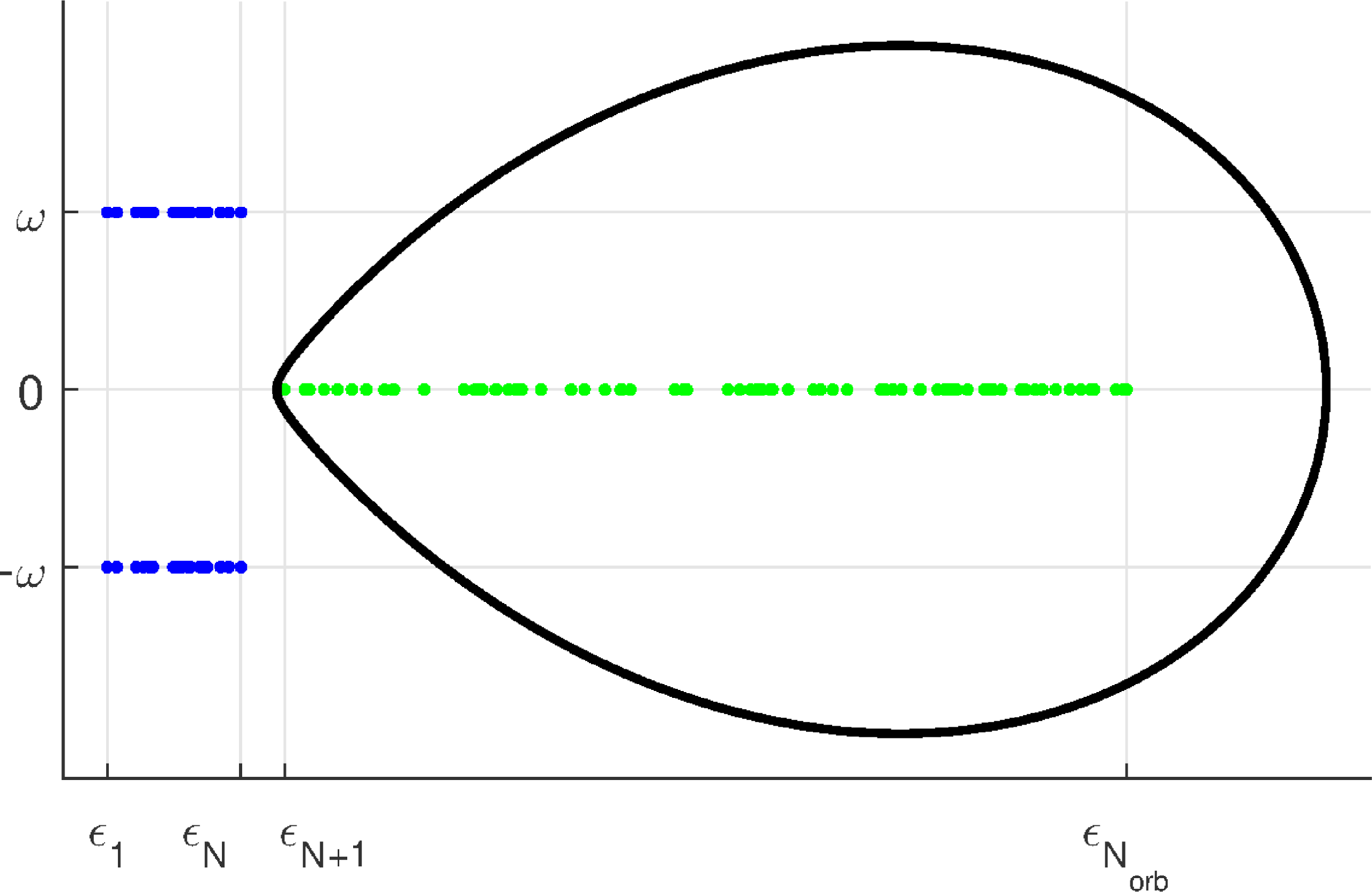
After we choose the contour
 $\mathscr{C}$
and apply Cauchy’s integral formula to split up the dependence of
 $i$
and
 $a$
in the denominator of (6.16), we obtain a reformulation for
 $\hat{\unicode[STIX]{x1D712}}^{0}$
which can be computed in cubic time complexity,
 $$\begin{eqnarray}\displaystyle \langle \mathbf{r}|\hat{\unicode[STIX]{x1D712}}^{0}(\text{i}\unicode[STIX]{x1D714})|\mathbf{r}^{\prime }\rangle & = & \displaystyle \mathop{\sum }_{i}^{\text{occ}}\mathop{\sum }_{a}^{\text{vir}}\displaystyle \frac{\unicode[STIX]{x1D713}_{i}^{\ast }(\mathbf{r})\unicode[STIX]{x1D713}_{a}(\mathbf{r})\unicode[STIX]{x1D713}_{a}^{\ast }(\mathbf{r}^{\prime })\unicode[STIX]{x1D713}_{i}(\mathbf{r}^{\prime })}{\unicode[STIX]{x1D700}_{j}-\unicode[STIX]{x1D700}_{k}-\text{i}\unicode[STIX]{x1D714}}+\text{c.c.}\nonumber\\ \displaystyle & = & \displaystyle \displaystyle \frac{1}{2\unicode[STIX]{x1D70B}\text{i}}\oint _{\mathscr{C}}\biggl(\mathop{\sum }_{i}^{\text{occ}}\displaystyle \frac{\unicode[STIX]{x1D713}_{i}^{\ast }(\mathbf{r})\unicode[STIX]{x1D713}_{i}(\mathbf{r}^{\prime })}{\unicode[STIX]{x1D706}-\unicode[STIX]{x1D700}_{i}+\text{i}\unicode[STIX]{x1D714}}\biggr)\biggl(\mathop{\sum }_{a}^{\text{vir}}\displaystyle \frac{\unicode[STIX]{x1D713}_{a}(\mathbf{r})\unicode[STIX]{x1D713}_{a}^{\ast }(\mathbf{r}^{\prime })}{\unicode[STIX]{x1D706}-\unicode[STIX]{x1D700}_{a}}\biggr)\,\text{d}\unicode[STIX]{x1D706}+\text{c.c.}\end{eqnarray}$$
Similar to that discussed in the case of PEXSI (see Section 5.3), the contour integral can be discretized and the number of quadrature points is logarithmic in
 $(\unicode[STIX]{x1D700}_{N_{\text{orb}}}-\unicode[STIX]{x1D700}_{N})/(\unicode[STIX]{x1D700}_{N+1}-\unicode[STIX]{x1D700}_{N})$
; we refer readers to Lu and Thicke (Reference Lu and Thicke2017a
) for details.
Note that the formula (6.19) already provides a cubic scaling method for calculating
 $\unicode[STIX]{x1D712}^{0}(\text{i}\unicode[STIX]{x1D714})$
. In particular, ignoring logarithmic factors,
 $\unicode[STIX]{x1D712}^{0}(\text{i}\unicode[STIX]{x1D714})$
can be calculated with cost
 $O(N_{\text{orb}}N_{g}^{2})$
, assuming we keep
 $N_{\text{orb}}$
total orbitals in the summation (known as the virtual orbital cut-off). However, the number of grid points
 $N_{g}$
could be much larger than the number of orbitals
 $N_{\text{orb}}$
. This motivates the use of ISDF to reduce the prefactor in the computational cost. We approximate the
 $\hat{\unicode[STIX]{x1D712}}^{0}$
operator by an operator
 $\tilde{\unicode[STIX]{x1D712}}^{0}$
by using the ISDF approximation:
 $$\begin{eqnarray}\displaystyle & & \displaystyle \langle \mathbf{r}|\hat{\unicode[STIX]{x1D712}}^{0}(\text{i}\unicode[STIX]{x1D714})|\mathbf{r}^{\prime }\rangle \nonumber\\ \displaystyle & & \displaystyle =\displaystyle \frac{1}{2\unicode[STIX]{x1D70B}\text{i}}\oint _{\mathscr{C}}\biggl(\mathop{\sum }_{i}^{\text{occ}}\displaystyle \frac{\unicode[STIX]{x1D713}_{i}^{\ast }(\mathbf{r})\unicode[STIX]{x1D713}_{i}(\mathbf{r}^{\prime })}{\unicode[STIX]{x1D706}-\unicode[STIX]{x1D700}_{i}+\text{i}\unicode[STIX]{x1D714}}\biggr)\biggl(\mathop{\sum }_{a}^{\text{vir}}\displaystyle \frac{\unicode[STIX]{x1D713}_{a}(\mathbf{r})\unicode[STIX]{x1D713}_{a}^{\ast }(\mathbf{r}^{\prime })}{\unicode[STIX]{x1D706}-\unicode[STIX]{x1D700}_{a}}\biggr)\,\text{d}\unicode[STIX]{x1D706}+\text{c.c.}\nonumber\\ \displaystyle & & \displaystyle \approx \mathop{\sum }_{\unicode[STIX]{x1D707}\unicode[STIX]{x1D708}}\displaystyle \frac{1}{2\unicode[STIX]{x1D70B}\text{i}}\oint _{\mathscr{C}}\biggl(\mathop{\sum }_{i}^{\text{occ}}\displaystyle \frac{\unicode[STIX]{x1D713}_{i}^{\ast }(\hat{\mathbf{r}}_{\unicode[STIX]{x1D707}})\unicode[STIX]{x1D713}_{i}(\hat{\mathbf{r}}_{\unicode[STIX]{x1D708}})}{\unicode[STIX]{x1D706}-\unicode[STIX]{x1D700}_{i}+\text{i}\unicode[STIX]{x1D714}}\biggr)\biggl(\mathop{\sum }_{a}^{\text{vir}}\displaystyle \frac{\unicode[STIX]{x1D713}_{a}(\hat{\mathbf{r}}_{\unicode[STIX]{x1D707}})\unicode[STIX]{x1D713}_{a}^{\ast }(\hat{\mathbf{r}}_{\unicode[STIX]{x1D708}})}{\unicode[STIX]{x1D706}-\unicode[STIX]{x1D700}_{a}}\biggr)\,\text{d}\unicode[STIX]{x1D706}\,\unicode[STIX]{x1D701}_{\unicode[STIX]{x1D707}}(\mathbf{r})\unicode[STIX]{x1D701}_{\unicode[STIX]{x1D708}}(\mathbf{r}^{\prime })+\text{c.c.}\nonumber\\ \displaystyle & & \displaystyle =:\mathop{\sum }_{\unicode[STIX]{x1D707}\unicode[STIX]{x1D708}}\unicode[STIX]{x1D712}_{\unicode[STIX]{x1D707}\unicode[STIX]{x1D708}}^{0}(\text{i}\unicode[STIX]{x1D714})\unicode[STIX]{x1D701}_{\unicode[STIX]{x1D707}}(\mathbf{r})\unicode[STIX]{x1D701}_{\unicode[STIX]{x1D708}}(\mathbf{r}^{\prime })=:\langle \mathbf{r}|\tilde{\unicode[STIX]{x1D712}}^{0}(\text{i}\unicode[STIX]{x1D714})|\mathbf{r}^{\prime }\rangle ,\end{eqnarray}$$
where the last line defines
 $\unicode[STIX]{x1D712}_{\unicode[STIX]{x1D707}\unicode[STIX]{x1D708}}^{0}$
and
 $\tilde{\unicode[STIX]{x1D712}}^{0}$
. We note that in the above the separability of the ISDF coefficients into the
 $i$
and
 $a$
components is crucial. Without this separability (e.g. if a conventional density fitting were used) we would not be able to calculate
 $\tilde{\unicode[STIX]{x1D712}}^{0}$
in cubic time since the sums over
 $i$
and
 $a$
would not decouple.
We now return our attention to the RPA correlation energy under random phase approximation (2.49). Given
 $\tilde{\unicode[STIX]{x1D712}}^{0}$
sufficiently close to
 $\hat{\unicode[STIX]{x1D712}}^{0}$
, we can approximate
 $\operatorname{Tr}[\ln (I-\hat{\unicode[STIX]{x1D712}}^{0}v_{C})]$
using (with a suitable choice of constant
 $c$
for convergence of the series)
 $$\begin{eqnarray}\displaystyle \ln (I-\tilde{\unicode[STIX]{x1D712}}^{0}v_{C}) & = & \displaystyle \ln [cI-((c-1)I+\tilde{\unicode[STIX]{x1D712}}^{0}v_{C})]\nonumber\\ \displaystyle & = & \displaystyle \ln (c)I+\ln \bigg[I-\displaystyle \frac{1}{c}((c-1)I+\tilde{\unicode[STIX]{x1D712}}^{0}v_{C})\bigg]\nonumber\\ \displaystyle & = & \displaystyle \ln (c)I-\mathop{\sum }_{\ell =1}^{\infty }\displaystyle \frac{[(c-1)I+\tilde{\unicode[STIX]{x1D712}}^{0}v_{C}]^{\ell }}{\ell c^{\ell }}\nonumber\\ \displaystyle & = & \displaystyle \ln (c)I-\mathop{\sum }_{\ell =1}^{\infty }\displaystyle \frac{1}{\ell c^{\ell }}\mathop{\sum }_{p=0}^{\ell }\binom{\ell }{p}(c-1)^{\ell -p}(\tilde{\unicode[STIX]{x1D712}}^{0}v_{C})^{p},\end{eqnarray}$$
and represent each the polynomial in terms of
 $\tilde{\unicode[STIX]{x1D712}}^{0}v_{C}$
on the right-hand side in the auxiliary basis. After some manipulation, this results in our final desired approximation,
 $$\begin{eqnarray}\operatorname{Tr}[\ln (1-\hat{\unicode[STIX]{x1D712}}^{0}(\text{i}\unicode[STIX]{x1D714})v_{C})+\hat{\unicode[STIX]{x1D712}}^{0}(\text{i}\unicode[STIX]{x1D714})v_{C}]\approx \operatorname{Tr}[\ln (1-\unicode[STIX]{x1D712}^{0}(\text{i}\unicode[STIX]{x1D714})v)+\unicode[STIX]{x1D712}^{0}(\text{i}\unicode[STIX]{x1D714})v],\end{eqnarray}$$
where
 $\unicode[STIX]{x1D712}^{0}$
and
 $v$
are the matrix elements in the auxiliary basis.
We present the cubic scaling algorithm for the calculation of the RPA correlation energy as in Algorithm 10. Details of the algorithm can be found in Lu and Thicke (Reference Lu and Thicke2017a ).

Our numerical results use the following test problem. Our two-dimensional spatial grid is
 $10\times 10N$
equally spaced points. First, we solve for the Kohn–Sham orbitals of the periodic system with an external potential consisting of
 $N$
Gaussian potential wells, the centres of which are randomly perturbed from the centres of their respective
 $10\times 10$
box of grid points. Then the eigenvectors of
 $H$
are used as the orbitals in the calculation of the RPA correlation energy.
We investigate the cubic scaling behaviour of the algorithm in Figure 6.2. The quartic scaling method using traditional density fitting is also plotted for comparison. In this example, we choose the virtual orbital cut-off
 $N_{\text{orb}}=0.2N_{g}$
and the system size is scaled up to
 $N=160$
. We observe that the cubic scaling algorithm greatly outperforms the quartic scaling algorithm for large system sizes.
(Credit: Lu and Thicke Reference Lu and Thicke2017a
.) Timing results for the quartic scaling method are plotted with solid lines, and results for the cubic scaling method are plotted with dashed lines. For reference, the purple and green dotted lines represent the slopes of
 $N^{4}$
and
 $N^{3}$
respectively. (a) Comparison of the time required to calculate
 $\unicode[STIX]{x1D712}^{0}$
and the time to perform the respective density fitting schemes for each method. (b) The total running time to calculate
 $E_{\text{c}}^{\text{RPA}}$
for each method.
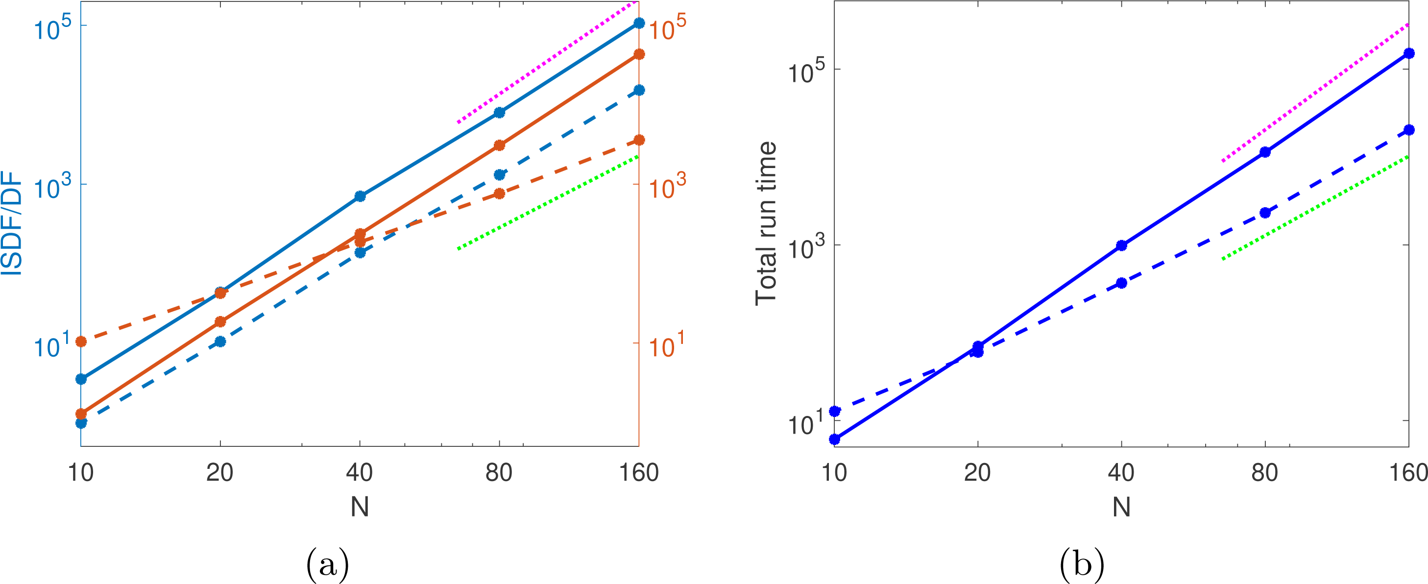
7 Self-consistent field iteration
In this section we discuss numerical methods for performing self-consistent field (SCF) iterations. In Sections 7.1 and 7.2 we introduce basic SCF iteration techniques such as the fixed-point iteration and the simple mixing method, as well as acceleration techniques based on Newton and quasi-Newton methods. We introduce these techniques in the context of semi-local functionals. In Section 7.3 we discuss preconditioning techniques for SCF iterations specific to semi-local functionals using a large basis set. Similarly Section 7.4 introduces SCF techniques specifically for non-local functionals. Throughout the discussion, we will assume a large basis set is used.
7.1 Fixed-point iteration and simple mixing
For a fixed atomic configuration, the self-consistent iteration starts from certain initial electron density denoted by
 $\unicode[STIX]{x1D70C}_{0}$
. We let
 $\unicode[STIX]{x1D70C}_{k},V_{k}$
denote the electron density and the effective potential
 $V_{\text{eff}}$
at the
 $k$
th SCF iteration, respectively. When pseudopotentials are used, since the non-local pseudopotential is independent of
 $\unicode[STIX]{x1D70C}$
,
 $V_{\text{eff}}$
is still a local potential as in equation (2.91). Then the flow of the SCF iteration becomes
 $$\begin{eqnarray}\cdots \rightarrow \unicode[STIX]{x1D70C}_{k}\rightarrow V_{k}=V_{\text{eff}}[\unicode[STIX]{x1D70C}_{k}]\rightarrow \unicode[STIX]{x1D70C}_{k+1}\rightarrow V_{k+1}=V_{\text{eff}}[\unicode[STIX]{x1D70C}_{k+1}]\rightarrow \cdots .\end{eqnarray}$$
Depending on the starting point, the relation (7.1) can be viewed as a mapping from
 $\unicode[STIX]{x1D70C}_{k}$
to
 $\unicode[STIX]{x1D70C}_{k+1}$
, or from
 $V_{k}$
to
 $V_{k+1}$
. The former viewpoint is called density mixing, while the latter is called potential mixing. There is no qualitative difference between the two types of mixing schemes. However, the density mixing has the extra constraint that the density must be non-negative everywhere, and must be normalized to have the correct number of electrons. In practice, this constraint can be easily satisfied by setting all the negative entries of
 $\unicode[STIX]{x1D70C}$
(usually these entries have very small magnitude) to
 $0$
or a small positive number, followed by a normalization step. On the other hand, potential mixing is formally free of such constraints, and hence we will consider potential mixing below. We remark that both density mixing and potential mixing strategies are widely used in electronic structure software packages, and the algorithm below for potential mixing can be used for density mixing as well.
When self-consistency is reached, the converged effective potential is denoted by
 $V_{\star }$
and satisfies the nonlinear equation
 $$\begin{eqnarray}V_{\star }=V_{\text{eff}}[{\mathcal{F}}_{\text{KS}}[V_{\star }]].\end{eqnarray}$$
The simplest version of the SCF iteration is the fixed-point iteration, where the potential at the
 $(k+1)$
th step is directly given by the output potential at the
 $k$
th step:
 $$\begin{eqnarray}V_{k+1}=V_{\text{eff}}[{\mathcal{F}}_{\text{KS}}[V_{k}]].\end{eqnarray}$$
Since the exchange-correlation functional is neither convex nor concave with respect to the electron density, rigorous study of the global convergence properties of SCF schemes in Kohn–Sham DFT calculations is difficult. Hence we consider the linear response regime, where we assume the initial effective potential
 $V_{0}$
is already close to
 $V_{\star }$
. Let
 $$\begin{eqnarray}e_{k}:=V_{k}-V_{\star }\end{eqnarray}$$
be the error of the potential at the
 $k$
th iteration. In order to study the propagation of the error in the fixed-point iteration (7.3), we apply the chain rule
 $$\begin{eqnarray}e_{k+1}=f_{\text{Hxc}}\unicode[STIX]{x1D712}_{0}e_{k}+O(\Vert e_{k}\Vert ^{2}).\end{eqnarray}$$
Here
 $f_{\text{Hxc}}=\unicode[STIX]{x1D6FF}V_{\text{eff}}/\unicode[STIX]{x1D6FF}\unicode[STIX]{x1D70C}$
is the kernel for the Hartree and exchange-correlation contributions, and
 $\unicode[STIX]{x1D712}_{0}=\unicode[STIX]{x1D6FF}{\mathcal{F}}_{\text{KS}}/\unicode[STIX]{x1D6FF}V$
is called the independent particle polarizability operator. In the linear response regime, we assume the
 $O(\Vert e_{k}\Vert ^{2})$
term is small and it is omitted in the following discussion. Then after
 $k$
steps
 $$\begin{eqnarray}e_{k}\approx (f_{\text{Hxc}}\unicode[STIX]{x1D712}_{0})^{k}e_{0}.\end{eqnarray}$$
Hence in the linear response regime, the convergence of the fixed-point iteration requires that the spectral radius of the operator, denoted by
 $r_{\unicode[STIX]{x1D70E}}(f_{\text{Hxc}}\unicode[STIX]{x1D712}_{0})$
, is smaller than
 $1$
. Unfortunately, such a spectral radius is generally much larger than
 $1$
, and the error in the fixed-point iteration will therefore diverge, even if the initial potential is already very close to the self-consistent potential.
In order to achieve the self-consistent solution, the simplest practically usable scheme is the simple mixing method, which introduces a slight modification of the fixed-point iteration, shown in Algorithm 11. The iteration can also be written equivalently as
 $$\begin{eqnarray}V_{k+1}=\unicode[STIX]{x1D6FC}V_{\text{eff}}[{\mathcal{F}}_{\text{KS}}[V_{k}]]+(1-\unicode[STIX]{x1D6FC})V_{k}.\end{eqnarray}$$

In the simple mixing method, the error propagation follows
 $$\begin{eqnarray}e_{k+1}=(I-\unicode[STIX]{x1D6FC}\unicode[STIX]{x1D716}_{d})e_{k}+O(\Vert e_{k}\Vert ^{2}).\end{eqnarray}$$
Here
 $\unicode[STIX]{x1D716}_{d}=I-f_{\text{Hxc}}\unicode[STIX]{x1D712}_{0}$
is called the dielectric operator. Equation (7.7) can be iterated, yielding
 $$\begin{eqnarray}e_{k}\approx (I-\unicode[STIX]{x1D6FC}\unicode[STIX]{x1D716}_{d})^{k}e_{0}.\end{eqnarray}$$
When the exchange-correlation functional contribution is dropped from
 $f_{\text{Hxc}}$
, the resulting approximation is called the random phase approximation (RPA).Footnote
1
Then
 $\unicode[STIX]{x1D716}_{d}$
can be transformed using a similarity transformation to a positive definite matrix. In particular,
 $\unicode[STIX]{x1D716}_{d}$
is diagonalizable with real positive eigenvalues. In order to achieve convergence in the linear response regime, we need each eigenvalue of
 $\unicode[STIX]{x1D716}_{d}$
, denoted by
 $\unicode[STIX]{x1D706}$
, to satisfy
 $$\begin{eqnarray}|1-\unicode[STIX]{x1D6FC}\unicode[STIX]{x1D706}|<1,\end{eqnarray}$$
or equivalently
 $$\begin{eqnarray}0<\unicode[STIX]{x1D6FC}<\displaystyle \frac{2}{\unicode[STIX]{x1D706}}.\end{eqnarray}$$
Let
 $\unicode[STIX]{x1D706}_{\min }$
and
 $\unicode[STIX]{x1D706}_{\max }$
denote the smallest and largest eigenvalues of
 $\unicode[STIX]{x1D716}_{d}$
, respectively, and the spectral radius
 $r_{\unicode[STIX]{x1D70E}}(\unicode[STIX]{x1D716}_{d})$
is then given by
 $\unicode[STIX]{x1D706}_{\max }$
. If
 $$\begin{eqnarray}0<\unicode[STIX]{x1D6FC}<\displaystyle \frac{2}{r_{\unicode[STIX]{x1D70E}}(\unicode[STIX]{x1D716}_{d})}\end{eqnarray}$$
is satisfied, the simple mixing would converge.
It remains to determine the optimal choice of
 $\unicode[STIX]{x1D6FC}$
satisfying the constraint (7.9). This requires the solution of the following minimax problem:
 $$\begin{eqnarray}\min _{\unicode[STIX]{x1D6FC}}\max _{\unicode[STIX]{x1D706}}|1-\unicode[STIX]{x1D6FC}\unicode[STIX]{x1D706}|.\end{eqnarray}$$
The optimal choice of
 $\unicode[STIX]{x1D6FC}$
satisfies
 $$\begin{eqnarray}1-\unicode[STIX]{x1D6FC}\unicode[STIX]{x1D706}_{\min }=\unicode[STIX]{x1D6FC}\unicode[STIX]{x1D706}_{\max }-1,\end{eqnarray}$$
or
 $$\begin{eqnarray}\unicode[STIX]{x1D6FC}=\displaystyle \frac{2}{\unicode[STIX]{x1D706}_{\min }+\unicode[STIX]{x1D706}_{\max }}.\end{eqnarray}$$
Substituting this choice of
 $\unicode[STIX]{x1D6FC}$
into (7.7), we find that the optimal convergence rate of simple mixing is
 $$\begin{eqnarray}\max _{\unicode[STIX]{x1D706}}|1-\unicode[STIX]{x1D6FC}\unicode[STIX]{x1D706}|=\displaystyle \frac{\unicode[STIX]{x1D706}_{\max }-\unicode[STIX]{x1D706}_{\min }}{\unicode[STIX]{x1D706}_{\max }+\unicode[STIX]{x1D706}_{\min }}=\displaystyle \frac{\unicode[STIX]{x1D705}(\unicode[STIX]{x1D716}_{d})-1}{\unicode[STIX]{x1D705}(\unicode[STIX]{x1D716}_{d})+1}.\end{eqnarray}$$
Here
 $\unicode[STIX]{x1D705}(\unicode[STIX]{x1D700}_{d})=\unicode[STIX]{x1D706}_{\max }/\unicode[STIX]{x1D706}_{\min }$
is the condition number of the dielectric operator.
In practical calculations, the condition number might be very large and the simple mixing method converges with a very slow rate. Thus the simple mixing method is rarely used directly in practical electronic structure calculations.
7.2 Newton and quasi-Newton type methods
The convergence of the simple mixing method often requires a rather small mixing constant
 $\unicode[STIX]{x1D6FC}$
. Hence the SCF procedure may take many iterations to converge. One possible acceleration can be achieved by using Newton’s method, which can be written as
 $$\begin{eqnarray}V_{k+1}=V_{k}-{\mathcal{J}}_{k}^{-1}r_{k}.\end{eqnarray}$$
Here
 ${\mathcal{J}}_{k}$
is the Jacobian matrix for the residual map
 $$\begin{eqnarray}\unicode[STIX]{x1D6FF}V\mapsto \unicode[STIX]{x1D6FF}V-V_{\text{eff}}[{\mathcal{F}}_{\text{KS}}[V_{k}+\unicode[STIX]{x1D6FF}V]].\end{eqnarray}$$
Note that at converged potential
 $V_{\star }$
, the Jacobian matrix
 ${\mathcal{J}}_{\star }=\unicode[STIX]{x1D716}_{d}$
. Hence the simple mixing method can also be interpreted as approximating the inverse of the Jacobian matrix
 ${\mathcal{J}}_{k}^{-1}$
simply by
 $\unicode[STIX]{x1D6FC}I$
in the evaluation of the Jacobian matrix for the composition map
 $V_{\text{eff}}\circ {\mathcal{F}}_{\text{KS}}$
. For a system with
 $N$
electrons, the evaluation of the Jacobian matrix requires in principle
 $O(N)$
evaluations of the Kohn–Sham map, which is prohibitively expensive.
The Jacobian-free Newton–Krylov method replaces the need for the explicit evaluation of the Jacobian matrix by solving a linear equation
 $$\begin{eqnarray}{\mathcal{J}}_{k}\unicode[STIX]{x1D6FF}V_{k}=-r_{k}\end{eqnarray}$$
to obtain the Newton update
 $\unicode[STIX]{x1D6FF}V_{k}$
. This can be done using iterative methods for solving linear equations, such as the generalized minimal residual method (GMRES) (Saad and Schultz Reference Saad and Schultz1986). In order to compute the matrix–vector multiplication related to the Jacobian matrix, one can use the finite difference approximation
 $$\begin{eqnarray}{\mathcal{J}}_{k}\unicode[STIX]{x1D6FF}V_{k}\approx \unicode[STIX]{x1D6FF}V_{k}-(V_{\text{eff}}[{\mathcal{F}}_{\text{KS}}[V_{k}+\unicode[STIX]{x1D6FF}V_{k}]]-V_{\text{eff}}[{\mathcal{F}}_{\text{KS}}[V_{k}]]).\end{eqnarray}$$
The finite difference calculation requires at least one additional function evaluation of
 ${\mathcal{F}}_{\text{KS}}(V_{k}+\unicode[STIX]{x1D6FF}V)$
per iteration step. Therefore, even though Newton’s method may exhibit local quadratic convergence, each Newton iteration may take many inner iterations in order to solve the linear equation (7.15).
A widely used alternative to Newton’s method is the class of quasi-Newton methods, which replace
 ${\mathcal{J}}_{k}^{-1}$
with an approximate matrix
 $C_{k}$
that is easy to compute and apply. Then the updating strategy becomes
 $$\begin{eqnarray}V_{k+1}=V_{k}-C_{k}r_{k}.\end{eqnarray}$$
Using Broyden’s techniques (Nocedal and Wright Reference Nocedal and Wright1999), one can systematically approximate
 ${\mathcal{J}}_{k}$
or
 ${\mathcal{J}}_{k}^{-1}$
. In Broyden’s second method,
 $C_{k}$
is obtained by performing a sequence of low-rank modifications to some initial approximation
 $C_{0}$
of the Jacobian inverse using a recursive formula (Fang and Saad Reference Fang and Saad2009, Marks and Luke Reference Marks and Luke2008). At each step,
 $C_{k}$
is obtained by solving the following constrained optimization problem:
 $$\begin{eqnarray}\displaystyle & & \displaystyle \min _{C}\displaystyle \frac{1}{2}\Vert C-C_{k-1}\Vert _{F}^{2}\nonumber\\ \displaystyle & & \displaystyle \;\text{subject to}~S_{k}=CY_{k},\end{eqnarray}$$
where
 $C_{k-1}$
is the approximation to the Jacobian constructed in the
 $(k-1)$
th Broyden iteration. The matrices
 $S_{k}$
and
 $Y_{k}$
above are defined as
 $$\begin{eqnarray}S_{k}=(s_{k},s_{k-1},\ldots ,s_{k-\ell }),\quad Y_{k}=(y_{k},y_{k-1},\ldots ,y_{k-\ell }),\end{eqnarray}$$
where
 $s_{j}$
and
 $y_{j}$
are defined by
 $s_{j}=V_{j}-V_{j-1}$
and
 $y_{j}=r_{j}-r_{j-1}$
respectively. The number
 $\ell$
is the length of history used in Broyden’s method, which is typically set to
 $5\sim 20$
in practical calculations.
Equation (7.18) is a constrained optimization problem and can be solved using the method of Lagrange multipliers, given by
 $$\begin{eqnarray}C_{k}=C_{k-1}+(S_{k}-C_{k-1}Y_{k})Y_{k}^{\dagger }.\end{eqnarray}$$
Here
 $Y_{k}^{\dagger }$
denotes the Moore–Penrose pseudo-inverse of
 $Y_{k}$
, that is,
 $Y_{k}^{\dagger }=(Y_{k}^{\ast }Y_{k})^{-1}Y_{k}^{\ast }$
. We remark that in practice
 $Y_{k}^{\dagger }$
is not constructed explicitly since we need only apply
 $Y_{k}^{\dagger }$
to a residual vector
 $r_{k}$
. This operation can be carried out by solving a linear least-squares problem with appropriate regularization (e.g. through a truncated singular value decomposition).
A variant of Broyden’s method is Anderson’s method (Anderson Reference Anderson1965), which is widely used in electronic structure software packages. Anderson’s method fixes
 $C_{k-1}$
to the initial approximation
 $C_{0}$
when solving (7.18) during each iteration. It follows from equation (7.17) that Anderson’s method updates the potential as
 $$\begin{eqnarray}V_{k+1}=V_{k}-C_{0}(I-Y_{k}Y_{k}^{\dagger })r_{k}-S_{k}Y_{k}^{\dagger }r_{k}.\end{eqnarray}$$
In particular, if
 $C_{0}$
is set to
 $\unicode[STIX]{x1D6FC}I$
, we obtain Anderson’s method,
 $$\begin{eqnarray}V_{k+1}=V_{k}-\unicode[STIX]{x1D6FC}(I-Y_{k}Y_{k}^{\dagger })r_{k}-S_{k}Y_{k}^{\dagger }r_{k},\end{eqnarray}$$
commonly used in Kohn–Sham DFT solvers. Pseudocode for Anderson’s method is shown in Algorithm 12.

An alternative way to derive Broyden’s method is through a technique called direct inversion of iterative subspace (DIIS). The technique was originally developed by Pulay to accelerate Hartree–Fock calculations (Pulay Reference Pulay1980). Hence it is often referred to as Pulay mixing. The motivation of Pulay’s method is to minimize the residual
 $V-V_{\text{eff}}[{\mathcal{F}}_{\text{KS}}(V)]$
within the subspace spanned by
 $\{V_{k-\ell -1},\ldots ,V_{k}\}$
. In Pulay’s original work (Pulay Reference Pulay1980), the optimal approximation to
 $V$
is expressed as
 $$\begin{eqnarray}V_{\text{opt}}=\mathop{\sum }_{j=k-\ell -1}^{k}\unicode[STIX]{x1D6FC}_{j}V_{j},\end{eqnarray}$$
where
 $V_{j}$
(
 $j=k-\ell -1,\ldots ,k$
) are previous approximations to
 $V$
, and the coefficients
 $\unicode[STIX]{x1D6FC}_{j}$
are chosen to satisfy the constraint
 $\sum _{j=k-\ell -1}^{k}\unicode[STIX]{x1D6FC}_{j}=1$
.
When the
 $V_{j}$
are all sufficiently close to the fixed-point solution,
 $$\begin{eqnarray}V_{\text{eff}}\bigg[{\mathcal{F}}_{\text{KS}}\biggl(\mathop{\sum }_{j}\unicode[STIX]{x1D6FC}_{j}V_{j}\biggr)\bigg]\approx \mathop{\sum }_{j}\unicode[STIX]{x1D6FC}_{j}V_{\text{eff}}[{\mathcal{F}}_{\text{KS}}(V_{j})]\end{eqnarray}$$
holds approximately. Hence we may obtain
 $\unicode[STIX]{x1D6FC}_{j}$
(and consequently
 $V_{\text{opt}}$
) by solving the following quadratic programming problem:
 $$\begin{eqnarray}\displaystyle & & \displaystyle \min _{\{\unicode[STIX]{x1D6FC}_{j}\}}\biggl\|\mathop{\sum }_{j=k-\ell -1}^{k}\unicode[STIX]{x1D6FC}_{j}r_{j}\biggr\|_{2}^{2}\nonumber\\ \displaystyle & & \displaystyle \;\text{subject to}~\mathop{\sum }_{j=k-\ell -1}^{k}\unicode[STIX]{x1D6FC}_{j}=1,\end{eqnarray}$$
where
 $r_{j}=V_{j}-V_{\text{eff}}[{\mathcal{F}}_{\text{KS}}(V_{j})]$
.
Note that (7.22) can be reformulated as an unconstrained minimization problem if
 $V_{\text{opt}}$
is required to take the form
 $$\begin{eqnarray}V_{\text{opt}}=V_{k}+\mathop{\sum }_{j=k-\ell }^{k}\unicode[STIX]{x1D6FD}_{j}(V_{j}-V_{j-1}),\end{eqnarray}$$
where
 $\unicode[STIX]{x1D6FD}_{j}$
can be any unconstrained real number. Again, if we assume
 $V_{\text{eff}}[{\mathcal{F}}_{\text{KS}}(V)]$
is approximately linear around
 $V_{j}$
and let
 $b=(\unicode[STIX]{x1D6FD}_{k-\ell },\ldots ,\unicode[STIX]{x1D6FD}_{k})^{\top }$
, minimizing
 $\Vert V_{\text{opt}}-V_{\text{eff}}[{\mathcal{F}}_{\text{KS}}(V_{\text{opt}})]\Vert$
with respect to
 $\{\unicode[STIX]{x1D6FD}_{j}\}$
yields
 $b=-Y_{k}^{\dagger }r_{k}$
, where
 $Y_{k}$
is the same as that defined in (7.19). Then Pulay’s method for updating
 $V$
is thus
 $V_{k+1}=V_{\text{opt}}$
. More generally, we may introduce a
 $C_{0}$
matrix as
 $$\begin{eqnarray}V_{k+1}=V_{\text{opt}}-C_{0}(V_{\text{opt}}-V_{\text{eff}}[{\mathcal{F}}_{\text{KS}}(V_{\text{opt}})]).\end{eqnarray}$$
Substituting
 $V_{\text{opt}}=V_{k}-S_{k}Y_{k}^{\dagger }r_{k}$
into (7.23), together with the linearity assumption of
 $V_{\text{eff}}[{\mathcal{F}}_{\text{KS}}(V)]$
, yields exactly Anderson’s updating formula (7.21).
The matrix
 $C_{0}$
plays the role of a preconditioner, and hence a better
 $C_{0}$
can be chosen to accelerate the convergence of Anderson’s method in practical electronic structure calculations, as will be discussed in Section 7.3.
It is worthwhile remarking that a variant of the Pulay method above can be derived by taking other definitions of the residual vector
 $r$
. This leads to the commutator-DIIS (C-DIIS) method (Pulay Reference Pulay1982), which defines the residual as the commutator of the Hamiltonian operator and the density matrix. This is the most widely used method in quantum chemistry software packages for achieving self-consistency. On the other hand, the C-DIIS method requires explicit storage of the density matrix and the Hamiltonian matrix for a few iterations, and hence is only feasible for calculations with small basis sets.
In the C-DIIS method, the residual, now written as
 $R$
, is the commutator between
 $H[P]$
and
 $P$
, that is,
 $$\begin{eqnarray}R[P]=H[P]P-PH[P].\end{eqnarray}$$
Note that the Hamiltonian matrix
 $H[P]$
and the effective potential
 $V_{\text{eff}}[P]$
contain the same information. Let
 $H_{k}$
denote the approximate Hamiltonian produced at step
 $k$
. We define a new Hamiltonian
 $\tilde{H}_{k+1}$
at step
 $(k+1)$
as a linear combination of previous approximations to the Hamiltonian, that is,
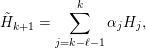 $$\begin{eqnarray}\tilde{H}_{k+1}=\mathop{\sum }_{j=k-\ell -1}^{k}\unicode[STIX]{x1D6FC}_{j}H_{j},\end{eqnarray}$$
where
 $\unicode[STIX]{x1D6FC}_{j}$
satisfies the constraint
 $\sum _{j=k-\ell -1}^{k}\unicode[STIX]{x1D6FC}_{j}=1$
. Each Hamiltonian matrix
 $H_{j}$
defines a density matrix
 $P_{j}$
via the generalized Kohn–Sham map. Before self-consistency is reached, the residual
 $R_{j}=R[P_{j}]$
defined by equation (7.24) is non-zero. However, when all the Hamiltonian matrices
 $\{H_{j}\}$
are close to the self-consistent Hamiltonian operator
 $H_{\star }$
, it is reasonable to expect the residual associated with
 $\tilde{H}_{k+1}$
to be well approximated by
 $\tilde{R}_{k+1}\equiv \sum _{j=k-\ell -1}^{k}\unicode[STIX]{x1D6FC}_{j}R_{j}$
. The C-DIIS method determines
 $\{\unicode[STIX]{x1D6FC}_{j}\}$
by minimizing
 $\tilde{R}_{k+1}$
, that is, we solve the following constrained minimization problem in each C-DIIS iteration:
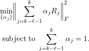 $$\begin{eqnarray}\displaystyle & & \displaystyle \min _{\{\unicode[STIX]{x1D6FC}_{j}\}}\biggl\|\mathop{\sum }_{j=k-\ell -1}^{k}\unicode[STIX]{x1D6FC}_{j}R_{j}\biggr\|_{F}^{2}\nonumber\\ \displaystyle & & \displaystyle \;\text{subject to}~\mathop{\sum }_{j=k-\ell -1}^{k}\unicode[STIX]{x1D6FC}_{j}=1.\end{eqnarray}$$
Here the Frobenius norm is defined as
 $\Vert A\Vert _{F}^{2}=\operatorname{Tr}[A^{\ast }A]$
.
As in the comparison between Anderson’s method and Pulay’s method above, the constraint in (7.26) can be eliminated by rewriting equation (7.25) as
 $$\begin{eqnarray}\tilde{H}_{k+1}=H_{k}+\mathop{\sum }_{j=k-\ell }^{k}\unicode[STIX]{x1D6FD}_{j}(H_{j-1}-H_{j}).\end{eqnarray}$$
Define
 $Y_{j}=R_{j-1}-R_{j}$
for
 $k-\ell +1\leq j\leq k$
. Then the constraint minimization problem (7.26) becomes an unconstrained minimization problem:
 $$\begin{eqnarray}\min _{\{\unicode[STIX]{x1D6FD}_{j}\}}\biggl\|R_{k}+\mathop{\sum }_{j=k-\ell +1}^{k}\unicode[STIX]{x1D6FD}_{j}Y_{j}\biggr\|_{F}^{2}.\end{eqnarray}$$
As a result, equation (7.28) has an analytic solution,
 $$\begin{eqnarray}\unicode[STIX]{x1D6FD}=-M^{-1}b,\end{eqnarray}$$
where the
 $\ell \times \ell$
matrix
 $M$
and the vector
 $b$
are defined as
 $$\begin{eqnarray}M_{ij}=\operatorname{Tr}[Y_{i}^{\ast }Y_{j}],\quad b_{j}=\operatorname{Tr}[Y_{j}^{\ast }R_{k}],\end{eqnarray}$$
respectively.
7.3 Preconditioning techniques
From the analysis of the simple mixing method we observe that the convergence rate is determined by the condition number of
 $\unicode[STIX]{x1D716}_{d}={\mathcal{J}}_{\star }$
. Hence we should examine the dependence of
 $\unicode[STIX]{x1D705}({\mathcal{J}}_{\star })$
with respect to the system size. Here we mainly examine periodic systems, of which the system size is often characterized by the number of unit cells in the computational domain. To simplify our discussion, we assume the unit cell to be a simple cubic cell with a lattice constant
 $L$
. For non-periodic systems such as molecules, we can construct a fictitious (cubic) supercell that encloses the molecule and periodically extend the supercell so that properties of the system can be analysed via Fourier analysis. In both cases, we assume the number of atoms in each supercell is proportional to
 $L^{3}$
.
When
 ${\mathcal{J}}_{\star }$
is similar to a positive definite matrix, the smallest eigenvalue
 $\unicode[STIX]{x1D706}_{\min }$
is often independent of the system size, but the largest eigenvalue
 $\unicode[STIX]{x1D706}_{\max }$
may depend sensitively on the system size. For instance, for the jellium system (or uniform electron gas),
 ${\mathcal{J}}_{\star }$
becomes a diagonal matrix in the Fourier space, and the eigenvalues can be evaluated explicitly as (Ziman Reference Ziman1979)
 $$\begin{eqnarray}\unicode[STIX]{x1D706}_{\mathbf{q}}=1+\biggl(\displaystyle \frac{4\unicode[STIX]{x1D70B}}{q^{2}}+\unicode[STIX]{x1D705}^{2}\biggr)\unicode[STIX]{x1D6FE}F_{L}(q),\quad \mathbf{q}\in \mathbb{R}^{3},\end{eqnarray}$$
where
 $q=|\mathbf{q}|$
,
 $\unicode[STIX]{x1D6FE},\unicode[STIX]{x1D705}$
are constants, and
 $F_{L}(q)$
is known as the Lindhard response function, which satisfies
 $$\begin{eqnarray}\lim _{q\rightarrow 0}F_{L}(q)=1,\quad \lim _{q\rightarrow \infty }F_{L}(q)=0.\end{eqnarray}$$
The above formulation is formally valid when the system size is infinite. Note that the smallest possible value
 $q$
is
 $2\unicode[STIX]{x1D70B}/L$
, and then
 $\unicode[STIX]{x1D706}_{\max }$
is bounded by
 $1+\unicode[STIX]{x1D6FE}(L^{2}/\unicode[STIX]{x1D70B}+\unicode[STIX]{x1D705}^{2})$
. As a result, the convergence of SCF iteration schemes becomes slower as the system size increases. If the mixing parameters are not adjusted properly, the long wavelength modes (corresponding to small
 $q$
) tend to be amplified as the SCF iteration proceeds. This phenomenon is called ‘charge sloshing’.
In order to accelerate the convergence, one can replace the scalar
 $\unicode[STIX]{x1D6FC}$
in the simple mixing method with a matrix
 $C_{0}$
, and the convergence rate is then determined by the condition number of the matrix
 $C_{0}{\mathcal{J}}_{\star }$
. As discussed in Section 7.2, the choice of the matrix
 $C_{0}$
in Anderson’s method plays the role of a preconditioner. The ideal preconditioner is
 $C_{0}={\mathcal{J}}_{\star }^{-1}$
as
 $\unicode[STIX]{x1D705}(C_{0}{\mathcal{J}}_{\star })=1$
. This corresponds to Newton’s method. To overcome charge sloshing, a widely used preconditioner is the Kerker preconditioner (Kerker Reference Kerker1981), which is much easier to apply. It assigns a smaller weight to the long wavelength Fourier modes in order to attenuate charge sloshing. More specifically, the Kerker preconditioner is a diagonal matrix in the Fourier space, and its eigenvalues are given by
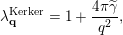 $$\begin{eqnarray}\unicode[STIX]{x1D706}_{\mathbf{q}}^{\text{Kerker}}=1+\displaystyle \frac{4\unicode[STIX]{x1D70B}\widetilde{\unicode[STIX]{x1D6FE}}}{q^{2}},\end{eqnarray}$$
where
 $\widetilde{\unicode[STIX]{x1D6FE}}>0$
is an adjustable parameter. For the uniform electron gas, the matrix
 $C_{0}{\mathcal{J}}_{\star }$
is a diagonal matrix in the Fourier space, and its eigenvalues are
 $$\begin{eqnarray}\widetilde{\unicode[STIX]{x1D706}}_{\mathbf{q}}=\displaystyle \frac{q^{2}+\unicode[STIX]{x1D6FE}F_{L}(q)(4\unicode[STIX]{x1D70B}+\unicode[STIX]{x1D705}^{2}q^{2})}{q^{2}+4\unicode[STIX]{x1D70B}\widetilde{\unicode[STIX]{x1D6FE}}}.\end{eqnarray}$$
The eigenvalue
 $\widetilde{\unicode[STIX]{x1D706}}_{\mathbf{q}}$
becomes approximately
 $1$
for large
 $q$
and
 $F_{L}(q)\unicode[STIX]{x1D6FE}/\widetilde{\unicode[STIX]{x1D6FE}}$
for small
 $q$
. Hence, after preconditioning, the eigenvalues can be bounded by constants independent of the system size. In practice it is found that the Kerker preconditioner is an effective preconditioner for simple metals such as sodium (Na) or aluminium (Al).
However, the Kerker preconditioner is not an appropriate preconditioner for insulating systems. Although in general the Jacobian associated with the insulating system cannot be diagonalized by the Fourier basis, it can be shown that
 $\text{e}^{\text{i}\mathbf{q}\cdot \mathbf{r}}$
is an approximate eigenfunction of the independent particle polarizability operator
 $\unicode[STIX]{x1D712}_{0}$
with the corresponding eigenvalue
 $-\unicode[STIX]{x1D709}q^{2}$
(Pick, Cohen and Martin Reference Pick, Cohen and Martin1970, Ghosez, Gonze and Godby Reference Ghosez, Gonze and Godby1997) for small
 $q$
, where
 $\unicode[STIX]{x1D709}>0$
is a constant factor. If we neglect the contribution from the exchange-correlation kernel,
 $\text{e}^{\text{i}\mathbf{q}\cdot \mathbf{r}}$
is also an approximate eigenfunction of
 ${\mathcal{J}}_{\star }$
with the corresponding eigenvalue
 $1+(4\unicode[STIX]{x1D70B}/q^{2})q^{2}\unicode[STIX]{x1D709}=1+4\unicode[STIX]{x1D70B}\unicode[STIX]{x1D709}$
for small
 $q$
. If
 $C_{0}$
is chosen to be the Kerker preconditioner, then the corresponding eigenvalue of
 $C_{0}{\mathcal{J}}_{\star }$
for small
 $q$
is approximately
 $$\begin{eqnarray}\widetilde{\unicode[STIX]{x1D706}}_{\mathbf{q}}=\displaystyle \frac{q^{2}}{q^{2}+4\unicode[STIX]{x1D70B}\widetilde{\unicode[STIX]{x1D6FE}}}(1+4\unicode[STIX]{x1D70B}\unicode[STIX]{x1D709}).\end{eqnarray}$$
As the system size
 $L$
increases, the smallest eigenvalue
 $\widetilde{\unicode[STIX]{x1D706}}_{\mathbf{q}}\sim L^{-2}$
, and thus the condition number
 $\unicode[STIX]{x1D705}(C_{0}{\mathcal{J}}_{\star })$
increases as the system size increases. For simple insulating systems, one good preconditioner is simply a constant, as the convergence of the simple mixing method is already independent of the system size.
As in the above discussion, simple insulating and metallic systems call for different types of preconditioners to accelerate the convergence of a fixed-point iteration for solving the Kohn–Sham problem. A natural question one may ask is how we should construct a preconditioner for a complex material that may contain both insulating and metallic components or metal surfaces. This leads to the elliptic preconditioner (Lin and Yang Reference Lin and Yang2013) as one promising strategy.
Note that under RPA (neglecting the exchange-correlation kernel), we may approximate
 ${\mathcal{J}}_{\star }^{-1}$
as
 $$\begin{eqnarray}\widetilde{{\mathcal{J}}}_{\star }^{-1}=(v_{C}^{-1}-\unicode[STIX]{x1D712}_{0})^{-1}v_{C}^{-1}.\end{eqnarray}$$
Since the Coulomb kernel
 $v_{C}^{-1}=-\unicode[STIX]{x1D6E5}/(4\unicode[STIX]{x1D70B})$
, applying
 $\widetilde{{\mathcal{J}}}_{\star }^{-1}$
to a residual vector
 $r_{k}$
simply amounts to solving the equation
 $$\begin{eqnarray}(-\unicode[STIX]{x1D6E5}-4\unicode[STIX]{x1D70B}\unicode[STIX]{x1D712}_{0})\tilde{r}_{k}=-\unicode[STIX]{x1D6E5}r_{k}.\end{eqnarray}$$
To construct a preconditioner, we will replace
 $\unicode[STIX]{x1D712}_{0}$
with a simpler operator. In many cases, we can choose the approximation to be a local (diagonal) operator defined by a function
 $b(\mathbf{r})$
, although other types of more sophisticated operators are possible. To compensate for the simplification of
 $\unicode[STIX]{x1D712}_{0}$
, we replace the Laplacian operator on the left of (7.35) by
 $-\unicode[STIX]{x1D6FB}\cdot (a(\mathbf{r})\unicode[STIX]{x1D6FB})$
for some appropriately chosen function
 $a(\mathbf{r})$
. This additional change yields the following elliptic PDE:
 $$\begin{eqnarray}(-\unicode[STIX]{x1D6FB}\cdot (a(\mathbf{r})\unicode[STIX]{x1D6FB})+4\unicode[STIX]{x1D70B}b(\mathbf{r}))\tilde{r}_{k}=-\unicode[STIX]{x1D6E5}r_{k}.\end{eqnarray}$$
Because our construction of the preconditioner involves solving an elliptic equation, equation (7.36) is called an elliptic preconditioner.
The elliptic preconditioner is naturally compatible with previous preconditioners for simple metals or insulators. For example, for uniform electron gas, setting
 $a(\mathbf{r})=1$
and
 $b(\mathbf{r})=-\widetilde{\unicode[STIX]{x1D6FE}}$
for some constant
 $\widetilde{\unicode[STIX]{x1D6FE}}>0$
yields
 $$\begin{eqnarray}(-\unicode[STIX]{x1D6E5}+4\unicode[STIX]{x1D70B}\widetilde{\unicode[STIX]{x1D6FE}})\tilde{r}_{k}=-\unicode[STIX]{x1D6E5}r_{k}.\end{eqnarray}$$
The solution of the above equation is exactly the same as that produced by the Kerker preconditioner. For simple insulating system, setting
 $a(\mathbf{r})=\unicode[STIX]{x1D6FC}^{-1}$
and
 $b(\mathbf{r})=0$
yields
 $$\begin{eqnarray}-\unicode[STIX]{x1D6FC}^{-1}\unicode[STIX]{x1D6E5}\tilde{r}_{k}=-\unicode[STIX]{x1D6E5}r_{k}.\end{eqnarray}$$
The solution to the above equation is simply
 $$\begin{eqnarray}\tilde{r}_{k}=\unicode[STIX]{x1D6FC}r_{k}.\end{eqnarray}$$
Such a solution corresponds to simple mixing with a mixing parameter
 $\unicode[STIX]{x1D6FC}$
.
For a complex system that consists of both insulating and metallic components, it is desirable to choose approximations to
 $a(\mathbf{r})$
and
 $b(\mathbf{r})$
that are spatially dependent. The asymptotic behaviour of
 $\unicode[STIX]{x1D712}$
with respect to the sizes of both insulating and metallic systems suggests that
 $a(\mathbf{r})$
and
 $b(\mathbf{r})$
should be chosen to satisfy
 $a(\mathbf{r})\geq 1$
and
 $b(\mathbf{r})\geq 0$
.
The implementation of the elliptic preconditioner only requires solving an elliptic equation, for instance through an iterative linear solver, such as the conjugate gradient method. In particular, fast algorithms such as multigrid (Brandt Reference Brandt1977), the fast multipole method (FMM) (Greengard and Rokhlin Reference Greengard and Rokhlin1987), hierarchical matrix solvers (Hackbusch Reference Hackbusch1999) and hierarchical semi-separable (HSS) matrix solvers (Chandrasekaran, Gu and Pals Reference Chandrasekaran, Gu and Pals2006) can be used to solve (7.36) in
 $O(N)$
arithmetic operations.
7.4 Rung-
$4$
functionals

As discussed in Section 7.2, the C-DIIS method is the most widely used method for Kohn–Sham DFT calculations with non-local functionals using a small basis set, such as Gaussian-type orbitals and atomic orbitals. However, it requires the explicit storage of the density matrix and the Hamiltonian matrix, and thus cannot be used in the setting of a large basis set such as planewaves. On the other hand, one cannot simply take the output Kohn–Sham orbitals from one SCF iteration and use them as the input Kohn–Sham orbitals for the next SCF iteration. As analysed in Section 7.1, such a fixed-point iteration is vulnerable to large eigenvalues of the Jacobian matrix and can suffer from the ‘charge sloshing’ problem. In practice, the most commonly used method for converging Kohn–Sham DFT calculations with a large basis set is a two-level nested SCF procedure. This is implemented, for instance, in the Quantum ESPRESSO software package. The motivation for using a two-level SCF procedure is to apply advanced charge mixing schemes to the electron density in the inner iteration to mitigate charge sloshing, and to use a fixed-point iteration to update the Kohn–Sham orbitals and consequently the exchange potential in the outer iteration. The update of the exchange potential is more costly, even though its contribution to total energy is typically much smaller.

The two-level nested SCF method is summarized in Algorithm 13. In each outer iteration, the exchange operator
 $V_{X}[P]$
is updated. This is implicitly done by updating a set of orbitals
 $\{\unicode[STIX]{x1D711}_{i}\}_{i=1}^{N}$
defining the density matrix as
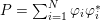 $P=\sum _{i=1}^{N}\unicode[STIX]{x1D711}_{i}\unicode[STIX]{x1D711}_{i}^{\ast }$
. We remark that this set of orbitals may be different from the Kohn–Sham orbitals in the inner SCF iteration. The update is done through a fixed-point iteration, that is,
 $\{\unicode[STIX]{x1D711}_{i}\}_{i=1}^{N}$
are given by the output Kohn–Sham orbitals in the previous outer iteration. In the inner SCF iteration, with the exchange operator fixed, the Hamiltonian
 $H$
depends only on the electron density
 $\unicode[STIX]{x1D70C}$
. Charge mixing schemes for
 $\unicode[STIX]{x1D70C}$
can be performed in a similar fashion to what is done in a standard Kohn–Sham DFT calculation without the exchange operator in the inner SCF iteration. Finally, within each inner iteration, with both
 $P$
and
 $\unicode[STIX]{x1D70C}$
fixed, the Hartree–Fock-like equation becomes a linear eigenvalue problem and can be solved by an iterative eigensolver discussed in Section 4.2. The outer SCF iteration continues until convergence is reached, which can be monitored using the change in the exchange energy, for example.
Recently, a new method, called the projected commutator DIIS (PC-DIIS) method, has been introduced so that the C-DIIS method can be used for Kohn–Sham DFT calculations with non-local functionals performed with a large basis set (Hu, Lin and Yang Reference Hu, Lin and Yang2017b
). Since it is not possible to explicitly store or mix the density matrices in such calculations, it is tempting to perform the DIIS procedure on the
 $N_{b}\times N$
orbital matrix
 $\unicode[STIX]{x1D6F9}=[\unicode[STIX]{x1D713}_{1},\ldots ,\unicode[STIX]{x1D713}_{N}]$
. However, one key difference between the density matrix and the orbital matrix is that the former is gauge-invariant. That is, if we replace
 $\unicode[STIX]{x1D6F9}$
with
 $\unicode[STIX]{x1D6F9}U$
, where
 $U$
is an
 $N\times N$
unitary gauge matrix, the density matrix
 $P=\unicode[STIX]{x1D6F9}\unicode[STIX]{x1D6F9}^{\ast }=\unicode[STIX]{x1D6F9}UU^{\ast }\unicode[STIX]{x1D6F9}^{\ast }$
does not change. Therefore, it is completely safe to combine two density matrices constructed from
 $\unicode[STIX]{x1D6F9}$
that differ by a gauge transformation, as the total energy is gauge-invariant.
However, since the orbital matrix
 $\unicode[STIX]{x1D6F9}$
is not gauge-invariant, combining successive approximations to
 $\unicode[STIX]{x1D6F9}$
that differ by a gauge transformation may hinder the stability of the SCF iteration. To overcome this difficulty, we introduce an auxiliary orbital matrix
 $\unicode[STIX]{x1D6F7}$
that spans the same subspace spanned by
 $\unicode[STIX]{x1D6F9}$
. This orbital matrix is obtained by applying the orthogonal projection operator associated with
 $\unicode[STIX]{x1D6F9}$
to a reference orbital matrix
 $\unicode[STIX]{x1D6F7}_{\text{ref}}$
to be specified later. That is,
 $\unicode[STIX]{x1D6F7}$
is chosen to be
 $$\begin{eqnarray}\unicode[STIX]{x1D6F7}=P\unicode[STIX]{x1D6F7}_{\text{ref}}=\unicode[STIX]{x1D6F9}(\unicode[STIX]{x1D6F9}^{\ast }\unicode[STIX]{x1D6F7}_{\text{ref}}).\end{eqnarray}$$
We require
 $\unicode[STIX]{x1D6F7}_{\text{ref}}$
to be fixed throughout the entire SCF procedure. Note that
 $\unicode[STIX]{x1D6F7}$
is invariant to any gauge transformation applied to
 $\unicode[STIX]{x1D6F9}$
. Therefore, the auxiliary orbital matrices obtained in successive SCF iterations can be safely combined to produce a better approximation to the desired invariant subspace. The columns of
 $\unicode[STIX]{x1D6F7}$
are generally not orthogonal to each other. However, as long as the columns of
 $\unicode[STIX]{x1D6F7}$
are not linearly dependent, both
 $\unicode[STIX]{x1D6F9}$
and
 $\unicode[STIX]{x1D6F7}$
span the range of the density matrix
 $P$
, which can also be written as
 $$\begin{eqnarray}P=\unicode[STIX]{x1D6F7}(\unicode[STIX]{x1D6F7}^{\ast }\unicode[STIX]{x1D6F7})^{-1}\unicode[STIX]{x1D6F7}^{\ast }.\end{eqnarray}$$
The PC-DIIS method constructs a new approximation to
 $\unicode[STIX]{x1D6F7}$
in the
 $k$
th SCF iteration by taking a linear combination of the auxiliary orbital matrices
 $\unicode[STIX]{x1D6F7}_{k-\ell },\ldots ,\unicode[STIX]{x1D6F7}_{k}$
obtained in the most recent
 $\ell +1$
iterations, that is,
 $$\begin{eqnarray}\tilde{\unicode[STIX]{x1D6F7}}_{k+1}=\mathop{\sum }_{j=k-\ell }^{k}\unicode[STIX]{x1D6FC}_{j}\unicode[STIX]{x1D6F7}_{j}.\end{eqnarray}$$
The coefficients
 $\{\unicode[STIX]{x1D6FC}_{j}\}$
in (7.41) are determined by minimizing the residual associated with
 $\tilde{\unicode[STIX]{x1D6F7}}_{k+1}$
, which, under the assumption that
 $\unicode[STIX]{x1D6F7}_{j}$
are sufficiently close to the solution of the Kohn–Sham equations, is well approximated by
 $R\equiv \sum _{j=k-\ell }^{k}\unicode[STIX]{x1D6FC}_{j}R_{\unicode[STIX]{x1D6F7}_{j}}$
, where the residual associated with an auxiliary orbital matrix
 $\unicode[STIX]{x1D6F7}$
is defined by
 $$\begin{eqnarray}R_{\unicode[STIX]{x1D6F7}}=H[P]P\unicode[STIX]{x1D6F7}_{\text{ref}}-PH[P]\unicode[STIX]{x1D6F7}_{\text{ref}}=(H[P]\unicode[STIX]{x1D6F9})(\unicode[STIX]{x1D6F9}^{\ast }\unicode[STIX]{x1D6F7}_{\text{ref}})-\unicode[STIX]{x1D6F9}((H[P]\unicode[STIX]{x1D6F9})^{\ast }\unicode[STIX]{x1D6F7}_{\text{ref}}).\end{eqnarray}$$
Note that evaluation of the residual in equation (7.42) only requires multiplying
 $H[P]$
by
 $\unicode[STIX]{x1D6F9}$
and the multiplications of matrices of sizes
 $N_{b}\times N$
and
 $N\times N$
only. These operations are already used in iterative methods for computing the desired eigenvectors
 $\unicode[STIX]{x1D6F9}$
of
 $H$
. The PC-DIIS algorithm does not require
 $P,H[P]$
or
 $R$
to be constructed or stored explicitly.
An interesting observation is that if
 $\unicode[STIX]{x1D6F7}_{\text{ref}}=\unicode[STIX]{x1D6F9}$
then
 $\unicode[STIX]{x1D6F9}^{\ast }H[P]\unicode[STIX]{x1D6F9}$
is a diagonal matrix denoted by
 $\unicode[STIX]{x1D6EC}$
. Consequently, the projected commutator takes the form
 $$\begin{eqnarray}R_{\unicode[STIX]{x1D6F7}}=H[P]\unicode[STIX]{x1D6F9}-\unicode[STIX]{x1D6F9}\unicode[STIX]{x1D6EC}.\end{eqnarray}$$
This expression coincides with the standard definition of the residual associated with an approximate eigenpair
 $(\unicode[STIX]{x1D6EC},\unicode[STIX]{x1D6F9})$
. Hence the PC-DIIS method can also be viewed as an extension of an iterative eigensolver for nonlinear problems.
As in the reformulation of the constrained minimization problem into an unconstrained minimization problem in the C-DIIS method, the constrained minimization problem
 $$\begin{eqnarray}\displaystyle & & \displaystyle \min _{\{\unicode[STIX]{x1D6FC}_{j}\}}\biggl\|\mathop{\sum }_{j=k-\ell }^{k}\unicode[STIX]{x1D6FC}_{j}R_{\unicode[STIX]{x1D6F7}_{j}}\biggr\|_{F}^{2}\nonumber\\ \displaystyle & & \displaystyle \;\text{subject to}~\mathop{\sum }_{j=k-\ell }^{k}\unicode[STIX]{x1D6FC}_{j}=1,\end{eqnarray}$$
to be solved in the PC-DIIS method can also be reformulated as an unconstrained minimization problem. Using the same change of variable as that presented in Section 7.2, we can write
 $$\begin{eqnarray}\tilde{\unicode[STIX]{x1D6F7}}_{k+1}=\unicode[STIX]{x1D6F7}_{k}+\mathop{\sum }_{j=k-\ell +1}^{k}\unicode[STIX]{x1D6FD}_{j}(\unicode[STIX]{x1D6F7}_{j-1}-\unicode[STIX]{x1D6F7}_{j}).\end{eqnarray}$$
If we let
 $Y_{\unicode[STIX]{x1D6F7}_{j}}=R_{\unicode[STIX]{x1D6F7}_{j-1}}-R_{\unicode[STIX]{x1D6F7}_{j}}$
, the coefficients
 $\unicode[STIX]{x1D6FD}_{j}$
in (7.45) can be retrieved from the vector
 $\unicode[STIX]{x1D6FD}=-(M^{\unicode[STIX]{x1D6F7}})^{-1}b^{\unicode[STIX]{x1D6F7}}$
, where
 $$\begin{eqnarray}M_{ij}^{\unicode[STIX]{x1D6F7}}=\operatorname{Tr}[Y_{\unicode[STIX]{x1D6F7}_{i}}^{\ast }Y_{\unicode[STIX]{x1D6F7}_{j}}],\quad b_{j}^{\unicode[STIX]{x1D6F7}}=\operatorname{Tr}[Y_{\unicode[STIX]{x1D6F7}_{j}}^{\ast }R_{\unicode[STIX]{x1D6F7}_{k}}].\end{eqnarray}$$
Once
 $\tilde{\unicode[STIX]{x1D6F7}}_{k+1}$
is obtained, a density matrix associated with this orbital matrix is implicitly defined through equation (7.40). This implicitly defined density matrix allows us to construct a new Hamiltonian from which a new set of Kohn–Sham orbitals
 $\unicode[STIX]{x1D6F9}_{k+1}$
and auxiliary orbitals
 $\unicode[STIX]{x1D6F7}_{k+1}$
can be computed.
We now discuss how to choose the gauge-fixing matrix
 $\unicode[STIX]{x1D6F7}_{\text{ref}}$
. Note that in hybrid functional calculations, the contribution from the exchange operator is relatively small. Hence the density matrix associated with Kohn–Sham orbitals obtained from a DFT calculation that uses a local or semi-local exchange-correlation functional is already a good initial guess for the density matrix required in a hybrid functional calculation. Therefore, we may use these orbitals as
 $\unicode[STIX]{x1D6F7}_{\text{ref}}$
. Compared to the two-level nested loop structure, the PC-DIIS method only requires one level of SCF iteration. The PC-DIIS method is summarized in Algorithm 14.
The discussion above is applicable when
 $\unicode[STIX]{x1D6F9}$
only contains the occupied orbitals. When
 $\unicode[STIX]{x1D6F9}$
also involves the virtual orbitals, we use the fact that the density matrix defining the Fock exchange operator only involves the occupied orbitals, and we need only apply the PC-DIIS method to the occupied orbitals. We also remark that the PC-DIIS method is not yet applicable for finite temperature calculations with fractionally occupied orbitals.

8 Conclusion and future directions
In this paper, we have reviewed some basic aspects and recent developments of numerical strategies for solving Kohn–Sham DFT. Most of the numerical methods focus on large systems, either due to the presence of a large number of electrons (thousands to tens of thousands), or due to the use of a large basis set (such as the planewave basis set). In this sense, the numerical algorithms in this paper are more suitable for applications in quantum physics and materials science, which often favour a large basis set and relatively large system sizes. On the other hand, the quantum chemistry literature often favours a small basis set (such as Gaussian-type orbitals) and relatively small system sizes, partly due to their focus on post-Hartree–Fock and post-DFT methods, which can be much more accurate but also more costly than DFT calculations. Even so, we remark that there has been growing interest in large system sizes and large basis sets in quantum chemistry (Sun, Berkelbach, McClain and Chan Reference Sun, Berkelbach, McClain and Chan2017, Stoudenmire and White Reference Stoudenmire and White2017, Mardirossian, McClain and Chan Reference Mardirossian, McClain and Chan2018), and the methods or ideas reviewed in this paper may then become applicable as well.
Although many advanced numerical methods have been implemented in mature DFT software packages, there are still many outstanding challenges for solving Kohn–Sham DFT. Below we provide our own perspectives organized according to the contents of this review.
(1) Numerical discretization. The pseudopotential approximation greatly facilitated the efficient discretization of the Kohn–Sham Hamiltonian. Nonetheless, it is not a systematic approximation, and is regarded by many as one of the ‘artistic’ components for solving Kohn–Sham DFT. Efficient discretizations that allow efficient all-electron calculations to be performed accurately, such as the numerical atomic basis sets, wavelets, and recent development of the Gausslet basis set (White Reference White2017), are still very much of interest. A key challenge would be to effectively control the number of degrees of freedom, so that calculations can still be performed efficiently for large systems.
(2) Evaluation of the Kohn–Sham map with semi-local functionals. The cross-over point of linear scaling methods and reduced scaling methods over conventional cubic scaling methods is still large, especially for three-dimensional bulk systems. Note that some key factors affecting the cross-over point, such as the decay rate of the density matrix, are determined by physical systems under consideration rather than numerical algorithms. Hence one cannot realistically expect the cross-over point to be reduced to below several hundreds of atoms in general. Nonetheless, many physical processes, such as the battery degradation process, require large simulation of systems with thousands to tens of thousands of atoms. Therefore further improvement of numerical algorithms and their parallel scalability, particularly for metallic systems, may enable a wide range of applications beyond reach today.
(3) Evaluation of the Kohn–Sham map with non-local functionals. The applicability range of Kohn–Sham DFT is ultimately determined by the choice of exchange-correlation functionals, and an increasing number of numerical calculations are now performed using rung-
$4$
and rung-
$5$
functionals. In some sense, the precise form of these functionals is still under development and somewhat debated in the literature. For instance, the self-consistently screened hybrid functional (Brawand, Vörös, Govoni and Galli Reference Brawand, Vörös, Govoni and Galli2016) was only developed in recent years, and there is as yet no consensus on the formulation of self-consistent rung-
$5$
functionals. In particular, rung-
$5$
functionals are closely related to Green’s function methods such as those in the many-body perturbation theory (MBPT) (Hedin Reference Hedin1965, Onida, Reining and Rubio Reference Onida, Reining and Rubio2002), which are often treated as post-DFT methods. For strongly correlated systems, novel exchange-correlation functionals such as those based on the strictly correlated electron (SCE) limit (Seidl, Gori-Giorgi and Savin Reference Seidl, Gori-Giorgi and Savin2007, Malet and Gori-Giorgi Reference Malet and Gori-Giorgi2012) offer new perspectives on the design of exchange-correlation functionals, though they have yet to be shown to be effective for practically relevant chemical systems.(4) Self-consistent field iterations. For large-scale heterogeneous systems with a small or zero energy gap, the SCF iteration often converges slowly, or fails to converge at all. This is particularly problematic for geometry optimization and molecular dynamics simulation, where a large number of iterations need to be performed at each step. It remains challenging to design efficient and robust approaches for self-consistency for large-scale systems. From this perspective, optimization based algorithms with guaranteed reduction of energy at each step could be more effective and robust.
(5) Numerical analysis. Due to the nonlinearity of the exchange-correlation functional, numerical analysis of Kohn–Sham DFT can be very challenging. Much progress has been made for simplified models such as the Thomas–Fermi-type models and reduced Hartree–Fock models (see e.g. Cancès, Deleurence and Lewin Reference Cancès, Deleurence and Lewin2008, Cancès and Lewin Reference Cancès and Lewin2010, Cancès and Mourad Reference Cancès and Mourad2014). Even so, there are still many basic questions from numerical analysis that remain to be answered, such as the convergence analysis of self-consistent field iterations beyond the linear response regime.


Finally, we would like to emphasize again the fact that although ‘Kohn–Sham DFT’ has become synonymous with ‘electronic structure theory’ in many contexts, it is only one of the many branches of electronic structure theories. We have not touched upon most of the wavefunction methods in the quantum chemistry literature, nor the methods for excited states or time-dependent problems. The fact that Kohn–Sham DFT has become so widely used today is because it strikes the right balance between efficiency, accuracy and general applicability so far. This balance has been constantly reshaped together with the development of many other theories, and will continue to be further reshaped in the future. Let us mention two possibilities.
Recently, there has been rapid surge of interest in applying machine learning tools to electronic structure theories. In the past few years there has been considerable progress in building inter-atomic potentials, for which the quality can be comparable to a first-principles simulation (see e.g. Bartók, Payne and Csányi Reference Bartók, Payne and Csányi2010, Zhang et al. Reference Zhang, Han, Wang and Car2018). Although machine learning based methods will still require electronic structure calculations to generate the training data, it is possible that in future we will not need to perform a monolithic, long-time first-principles molecular dynamics simulation for a large system. Instead it may be efficient enough to perform long molecular dynamics calculations for many small- to medium-sized systems in parallel, or for large systems but at many discontinuous snapshots. This may enable DFT calculations on a massively parallel scale, and many large systems beyond reach today might then become feasible. It may also be possible to use machine learning tools to build better density functionals or to more efficiently solve DFT. The interaction between physical modelling, data and numerical algorithms promises to further improve the predictive power of electronic structure theories for materials and chemical systems.
Another possibility is the fusion of DFT methods with other physical theories. In the quantum physics and chemistry literature, such multiscale-like theories are called ‘quantum embedding theories’. Kohn–Sham DFT can be combined with more coarse-grained theories such as molecular mechanics to simulate large-scale systems such as biological systems. These ‘quantum mechanics / molecular mechanics’ (QM/MM) methods began in the 1970s (Warshel and Levitt Reference Warshel and Levitt1976) and were recognized by the Nobel Prize in Chemistry in 2013. Kohn–Sham DFT can also be combined with more accurate post-DFT methods, such as coupled cluster methods, density matrix renormalization group methods, quantum Monte Carlo methods and exact diagonalization methods (Sun and Chan Reference Sun and Chan2016, Georges, Kotliar, Krauth and Rozenberg Reference Georges, Kotliar, Krauth and Rozenberg1996, Kotliar et al. Reference Kotliar, Savrasov, Haule, Oudovenko, Parcollet and Marianetti2006, Knizia and Chan Reference Knizia and Chan2012, Manby, Stella, Goodpaster and Miller III Reference Manby, Stella, Goodpaster and Miller2012) to solve strongly correlated systems. As of today, these methods certainly still lack the ease of use and general applicability compared to Kohn–Sham DFT. There are challenges as well as opportunities for applied mathematicians to make contributions.
Notation