2. Data

The 2 per cent national sample of the 1851 census generated by Anderson and colleagues was at the time seen as a mammoth exercise in data collection and manipulation. The full dataset, which covered the censuses of both England and Wales, and Scotland, and included some 82,500 households and 400,000 individuals, was one of the largest of its kind. Yet for his Continuity and Change article, due to the complexities of coding and classification, a 1 in 2,000 household sub-sample of just 2,067 households and 9,828 individuals was abstracted from the full dataset. Much has changed due to increased and cheaper computer power and capacity in the past 30 years. The I-CeM data used in this article is not a sample, but rather a transcription of the complete census records that survive for the period 1851–1911. As a result, the English and Welsh elements of the I-CeM data collection currently extend to 38,662,750 households and 187,720,820 individuals, over 15,000 times the amount that was available to Anderson.Footnote ⁴ The sheer size of the I-CeM data collection brings its own complexities, but the greater temporal coverage and depth equally allows insights not previously available.

One of the strengths of I-CeM is that it is not just a raw transcription of the information contained within the census enumerators’ books. The information has been extensively coded and standardised to make subsequent analysis easier. In addition, the data has been enhanced by the addition of a series of derived and imputed variables based on the combination of individuals found within each household. Of particular importance in the case of this article, a program – much like the software package (CENDEP) used by Anderson for his sub-sample of 2,067 householdsFootnote ⁵ – has been developed in conjunction with the I-CeM data, which identifies, where possible, conjugal family units (CFUs) within households. This identifies offspring living with a parent or parents, regardless of headship.Footnote ⁶ While the vast majority of such CFUs are formed by a combination of Head, Spouse, Daughter(s) and/or Son(s), the program also allows for kin combinations where the senior member of the CFU is not a Head of household, for example, ‘Daughter, Son-in-Law and Grandchild’ or ‘Brother (widowed) and Niece’, as well CFUs formed within boarder and lodger groups in which these exist. The formation of CFUs is not just based on the designation of relationship to the head of the household, since it is important to undertake consistency checks using surnames, marital status and especially age difference between (potential) husband and wife pairs and parent and child pairs. In making such consistency checks, account was also taken of the possibility of ‘shifting’ relationships, when the recorded relation is not that relative to the head of household, but rather to the preceding person within the household. For example, ‘Head, Daughter, Daughter’ (where the second daughter is in fact a grand-daughter of the head) or ‘Head, Lodger, Daughter, Son’ (where the children are those of the lodger, not the head). While relatively rare, such practice is not unknown in the nineteenth-century CEBs.Footnote ⁷ Once completed, the allocation of CFUs is used to calculate the Hammel-Laslett typology of household classification,Footnote ⁸ as well as to generate a series of individual level variables that are important in the analysis of familial structures, indicating if individuals are resident with other categories of persons, such as mother, father, offspring, kin, servants, and so on.

Given the focus on households and families in this article, it is important to note that in the censuses in the second half of the nineteenth century there was some confusion over the identification of households.Footnote ⁹ For the censuses of the mid-nineteenth century, the census office promoted the notion of occupiers in relation to both households and families, defining the latter in 1851 as: ‘the persons under one head; who is the occupier of the house, the householder, master, husband, or father; while the other members of the family are, the wife, children, servants, relatives, visitors, and persons constantly or accidentally in the house’.Footnote ¹⁰

Leaving aside the expectation that heads of household – the occupier – would be male, which as analysis shows was not always the case, this definition is ambiguous about the position of boarders and lodgers. The former were usually taken as those who took meals with the main family, while the later were those who rented a room or rooms within the house but who functioned independently of the main family. In practice, a clear-cut division between boarders and lodgers was not possible. In 1851 census enumerators were instructed to leave a separate household schedule with each occupier, meaning ‘either the resident owner or any person who pays rent, whether (as a tenant) for the whole of a house or (as a lodger) for any distinct floor or apartment’. This did little to resolve the ambiguity over and distinction between lodgers and boarders, especially if they shared parts of the building/house with their landlord rather than having a distinct ‘floor or apartment’. The census of 1861 made an attempt to rectify this confusion by distinguishing between types of lodging, instructing enumerators to leave householder schedules: ‘for a family consisting of a man, his wife, and children, [or] of parents, children, servants and visitors; for a family consisting of parents and children, with boarders at the same table, and the servants of the family, if any; for a lodger alone, or two or more lodgers boarding together’. While this wording was undoubtedly clearer, the census office rather undermined this clarity by depicting a solitary lodger not only as part of a household attached to the main familial group, but also as a separate household in the exemplar illustrating how the CEBs were to be compiled. This was repeated in the two subsequent censuses and clearly created confusion with enumerators and householders alike, as was recognised in the Report of 1891:

Definitions and instructions were changed yet again in 1901, and repeated in 1911, in order to reinforce the view that lodgers, either alone or living with other lodgers should be treated as separate independent households, emphasised by the introduction of mechanical tabulation technology in 1911 which treated every separate schedule a de facto ‘household’ unit.Footnote ¹²

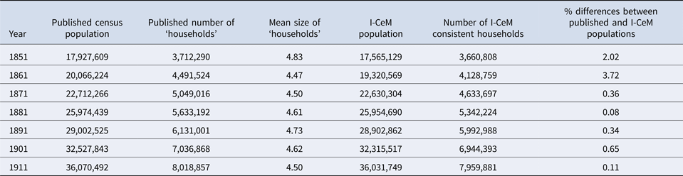
These multiple changes in definition mean that official census office data at the household level may not be consistent over the period under consideration, which may be one of the reasons why the Victorian Census Office published hardly any statistical tables with the household as the unit of observation.Footnote ¹³ The effect of these changing enumeration practices can be seen in Table 1, where ‘observed’ mean household sizes move, in part, in accordance with the prevailing way in which schedules were distributed and completed. Thus, in order to facilitate meaningful comparison over successive census years it is critically important to define household boundaries in as uniform a way as possible within the I-CeM data.Footnote ¹⁴ Rather than taking each schedule as a separate household regardless of census year, information across schedules has been amalgamated if the address on the successive schedules is the same and first named individual on the second (or subsequent) schedule is designated under relationship to head as either lodger/boarder/servant or visitor. The effect of this can be seen by comparing the ‘observed’ mean household sizes given in Table 1 with the modified means presented in Table 3, which are discussed later.

Table 1.

Population and household counts compared (1851–1911)

Note: The difference between the published census populations and the I-CeM populations (rightmost column) is mainly due to original manuscript census pages having been lost or destroyed. In 1851 and 1861 there are some cases of whole enumeration districts and parishes being affected.

Source: The 1851–1911 published population figures are taken from the 1921 census report, Census of England and Wales, 1921, Preliminary report including tables of the population enumerated in England and Wales (administrative and parliamentary areas) and in Scotland, the Isle of Man, and the Channel Islands on 19–20th June 1921. BPP 1921 XVI (Cmd.1485) 1. http://www.histpop.org/ohpr/servlet/PageBrowser?path=Browse/Census%20(by%20date)/1921&active=yes&mno=165&tocstate=expandnew&tocseq=1500&display=sections&display=tables&display=pagetitles&pageseq=first-nonblank [accessed 21 May 2017]. Note, in the nineteenth century the population totals given in retrospective census reports are invariably slightly different to the initial reports of the given census year because of subsequent corrections. The population counts in this table include institutions and well as ‘private’ households. It is impossible to tell from the published returns what the size of the institutional population was at any census. For a discussion of this issue, see text.

Clarification is also needed concerning the treatment of institutions in the censuses. In every census between 1851 and 1911 institutions were enumerated separately from ‘private’ households, yet included in the overall population counts (Table 1). However, what counted as an institution was inconsistent not only over different census years, but also within the same census, since the census office effectively identified institutions partly by function and partly by size.Footnote ¹⁵ Thus, for example, a hotel, boarding house, or prison, could be enumerated as either a ‘private’ household, or an institution depending on both the number size of persons it contained and the enumerator's discretion. Again, in order to facilitate comparisons between census years, in the I-CeM data every attempt has been made to identify and treat institutions consistently, according to function. Thus, various ‘private households’ enumerated in standard CEBs rather than in the special institution books have been re-designated as institutions.Footnote ¹⁶ In Tables 1–3, most take households or individuals within households as their denominator; individuals residing in institutions are therefore excluded, unless otherwise specifically mentioned.

Lastly, before moving to the analyses it is important to note that while the I-CeM data are voluminous, they are not totally complete. The extent of the data missing or, to use the archival term, ‘wanting’ in each year is shown in Table 1. The reasons for these discrepancies are mainly twofold: either the original CEBs have been lost or destroyed, partially or in full; or a CEB, or part of it – maybe a page or even a line here and there – was not transcribed. The worst year in terms in incompleteness is 1861 when it is known that a number of CEBs have been lost in their entirety, including in some cases complete Registration Sub-Districts, yet even this year is still over 96 per cent complete. For the purpose of the analyses presented here, the more important issue is whether the missing census tracts introduce any bias into the results. As far as it is possible to tell, the missing data seem to be entirely random.

3. A note on terminology

Before presenting results and findings, it is worth making some generic remarks about definitions and terminology. For the avoidance of confusion, this article uses terms in accordance with the definitions as set out in Laslett's 1972 essay on comparative household structure.Footnote ¹⁷ Consequently, a ‘household’ is defined as consisting of a head, plus a spouse if present, any co-resident children and other kin, as well as servants. The term ‘houseful’ is used to distinguish the household from the larger grouping of household plus other residents attached to but not within the household: namely boarders, lodgers and any visitors. Thus, housefuls can be larger than households. Any individuals residing in institutions, both private and public, are not considered in either the count of households or housefuls in subsequent tables and figures.

Any never-married children of a head and their spouse are designated by the term ‘offspring’, and are distinguished from ever-married children, who are treated as relatives. The term ‘relative’ includes all co-resident individuals specified as being related, who are neither spouse nor offspring of the head. The term ‘kin’ differs from relative in that the latter are co-resident with the head, whereas kin implies both co-resident and non-resident related individuals, and is thus a wider group (and one which is impossible to define precisely). ‘Servants’ are those seen to be in the employment of, and co-resident with, the head (or their spouse, offspring or relative). While live-in domestic servants are by far the majority in this category, it is a generic term that also includes, where relevant, live-in farm servants, apprentices, journeymen, journeywomen and other identifiable employees in the ‘service’ of the household. Another generic term that is used is ‘inmate’. This is defined as a person outside of the household, but attached to it in some residential and contractual way, essentially lodgers and boarders. ‘Visitors’, who are seen as temporary residents, are excluded from this category and treated separately from any other members of the co-resident group. Some previous detailed community-based studies reconstructing kin groups have demonstrated that some individuals who are identified as either visitor or servant in the Victorian CEBs were actually related to the head.Footnote ¹⁸ The same is most likely true of some inmates as well, but unfortunately it is impossible to say how widespread such cases were, or how such reporting may have changed over time. As a consequence, in the analyses that follow, all servants, visitors and inmates designated as such are treated as recorded on the basis that this is how the household head perceived them (and enumerator).

4. Fertility and mortality

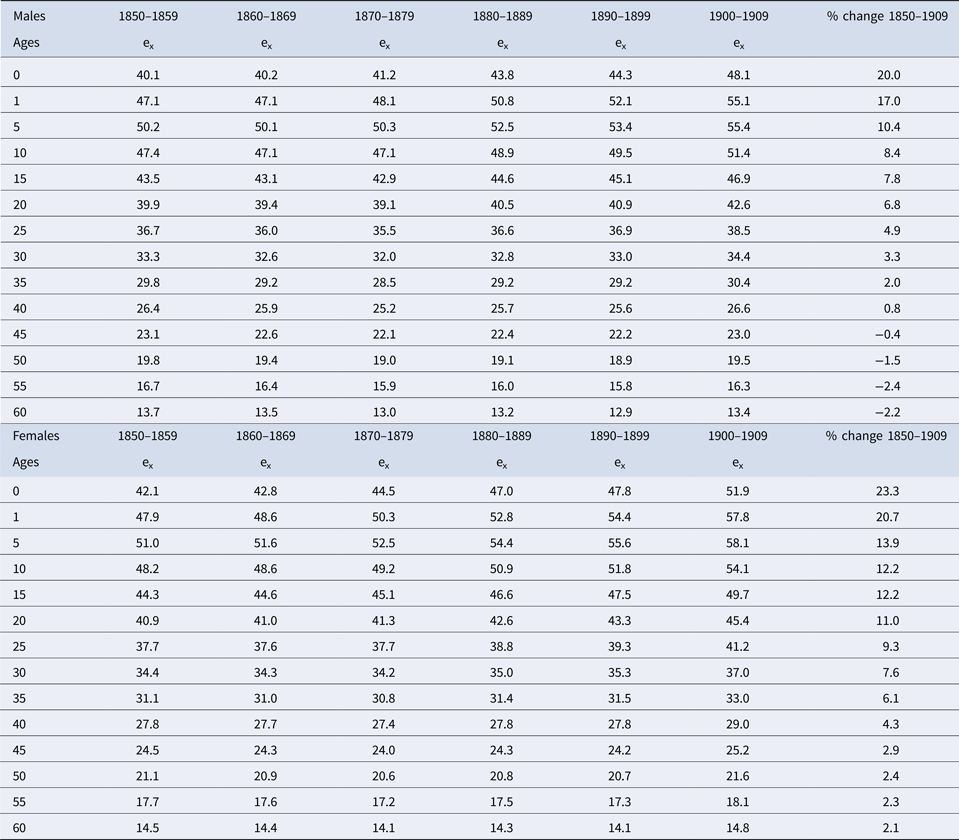
While the key subject matter of this article is household and family structures, clearly changes in the dynamics of household structure over time will be conditioned by the underlying mortality and fertility regimes. Consequently, in order to provide context to the discussion on family structures that follows, it is important to outline the key demographic changes in the period in question. At a national level, Table 2 summarises the improvement in mortality witnessed in the 60-year period. Expectation of life at birth (e ₀) for males remained relatively unchanged between the 1850s and the 1870s but thereafter fluctuated before improving at the end of the nineteenth century and beginning of the twentieth century, increasing by some 8 years from 40.1 in the 1850s to 48.1 in the period 1900–1909.Footnote ¹⁹ While the broad trend was similar, the expectation of life for females improved at a faster rate than for males, increasing by some 10.2 years from 42.1 years to 51.9, with the result that the differential mortality between the sexes increased gradually over the period, widening from 2 years in the 1850s to 3.8 years by the early twentieth century.Footnote ²⁰ However, these improvements in mortality were not even in terms of age structure. In general terms, improvement was initially the result of a decreasing mortality rates for children, adolescents and even those in their early twenties (5–24). This was followed by an improvement in adult mortality (25–39), initially for females, with adult male mortality (25–49) improving slightly in the last quarter of the century. While declines in the levels of child mortality were seen before the end of the century, one of the key contributors to life expectancy figures, infant mortality, did not start to decline significantly before the end of the century – but once underway, the decline was extremely rapid.Footnote ²¹

Table 2.

Expectation of life at key ages (e _x) (1850–1909)

Source: Human Mortality Database developed by the University of California, Berkeley (US) and the Max Planck Institute for Demographic Research (Germany), available at www.mortality.org [accessed 22 May 2017].

Turning to fertility, it is important first to consider nuptiality, which affects fertility through exposure to the risk of pregnancy. Marriage ages for men, as indicated by the Singulate Mean Age at Marriage (SMAM), rose gradually throughout the period, from 26.1 in 1851 to reach 26.6 by 1881, 27.2 by 1901, and a high of 27.6 by 1911. In comparison, the SMAM for women fell slightly between 1851 and 1861, from 25.5 to 25.2, then remained level before increasing to 25.8 in 1891 and 26.2 in 1901, after which point it remained level again through to 1911.Footnote ²² In conjunction with these changes in the age of marriage, the percentage of the population remaining unmarried aged 45–54 – which had risen steadily during the first half of the nineteenth century, to reach levels of around 11.7 and 11.2 for males and females respectively by 1851 – declined in the case of men from the mid-century to reach levels of around 9.3 in 1881, before rising steadily again to reach a level by 1911 similar to that of 1851 (11.8). The trajectory for females was slightly different, the percentage of never-married increasing very slightly from 1851–1911 (11.2 to 11.6), rising more sharply thereafter, reaching 15.6 by 1911.Footnote ²³ Thus, especially from 1881 through to 1911, higher ages of marriage were accompanied by high proportions of individuals never-marrying. Simultaneously, and unaffected by changes in nuptiality, marital fertility rates witnessed a steady decline, starting in the 1870s through to the end of the period of study and beyond, declining more sharply in the twentieth century. Therefore overall fertility levels, which are determined by both nuptiality and marital fertility, faced downward pressure from both these elements, particularly the latter.Footnote ²⁴

Mortality and fertility rates and patterns of nuptiality all varied geographically in this period, in some cases quite dramatically. However, as the focus in this article is essentially at the national level any detailed discussion of local and regional variation over time will not be considered. It is important, however, to make three general points.Footnote ²⁵ First, as might be expected, mortality levels tended to be higher in Victorian towns and cities relative to the countryside, but the relationship between population density and mortality levels was far from linear. Likewise, fertility levels were generally higher in agricultural areas and mining areas than in urban areas, but this broad generalisation needs to be tempered by consideration of class and place. Within high fertility areas, those in the professional classes tended to lower their fertility first; but place mattered too for them in that they lowered their fertility less than professionals living in low fertility areas. Similar qualifications could also be made in the case of mortality. Lastly, and this is probably the most important point for the discussion in this article, spatial differences in some cases narrowed over time, especially at the very end of the nineteenth century and turning into the twentieth.

This outline of the prevailing demographic trends between 1851 and 1911 helps us to understand their impact on household and family. Evidentially, residential household groups may be shaped as much by demographic possibility as by cultural or social desire or influence.Footnote ²⁶ Using demographic simulations, this point has been forcefully demonstrated by Zhongwei Zhao, who contrasted the experiences of a theoretical birth cohort from 1851 with one from 1901, to represent pre- and post-demographic transition regimes.Footnote ²⁷ He illustrated this point by demonstrating that in the 1851 birth cohort, some 10 per cent of girls would have lost both parents by the age of 10 through death, and 18 per cent would have done so by age 15. Sixty years on, improvements in mortality had reduced this figure to 2 per cent at age 10 with little further rise by age 15.Footnote ²⁸ Likewise, in relation to the possibility of children knowing their grandparents, by age 30, when many women were raising a family, only 34 per cent of the 1851 cohort had both parents alive, compared to 60 per cent of the later cohort.Footnote ²⁹ However, the demographic simulations also make it clear that higher fertility levels lead to higher overall kin availability, as measured by the mean number of kin an individual will have at different ages, in the pre-transition regime than in the post – significantly so for both lateral and descending kin, and marginally so for ascending kin.Footnote ³⁰ Thus, in the discussion of household and family experience that follows, some of the change described may have been driven by fluctuating demographic constraints and opportunities, yet it is important to realise that simply because kin exist does not necessarily mean that they had the possibility to actually live in the same household or to offer forms of support – migration, which as will be discussed below, increased over the period in question, would have separated families; and some family members may have been simply unwilling to live with or provide assistance to their relatives.Footnote ³¹

5. Household size

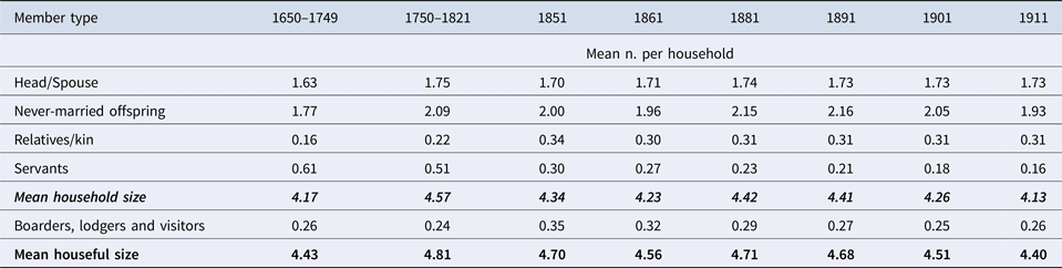
Table 3 presents the mean number of individuals in each of the most basic categories of household membership, adjusted where possible to reflect a consistent definition of household over time. This clearly demonstrates that in terms of household and houseful sizes the period 1851–1911 was one of relative stability. There was a small decline in the size of households, both with and without attached inmates and visitors, but this was quite slender: just over 5 per cent in the case of the former and some 6.5 per cent in the case of the latter. Comparing the I-CeM data with Laslett and Wall's ‘100 standard’ English communities for 1650 to 1821 also emphasises continuity rather than change, in many ways confirming Laslett's early suggestion that the English household was basically unchanged prior to the twentieth century. Perhaps ironically, in terms of measures of overall household size, the figures for 1911 were more like the data from 1650 to 1749 than those for 1851. The decline in household size was proportionally slightly greater between the selected communities for 1750–1821 and 1851 than it was between 1851 and 1911. Thus, if one is looking for a peak in English household sizes (since the early modern period) it is, perhaps unsurprisingly, in the period of rapid population growth between the late eighteenth and early nineteenth centuries that one should conduct the search. Overall mean household size remained relatively stable over the second half of the nineteenth century and not dramatically different from the historic ‘small’ household sizes gleaned from parish listings for the pre-nineteenth-century period. While household sizes in England and Wales today are almost half (47.5 per cent) of what they were at their recorded peak in 1750–1821, it is only as one enters the twentieth century that one sees household sizes beginning to fall significantly. Yet even then the decline was initially slow – household sizes fell by just 6.8 per cent between 1891 and 1911. Thereafter the pace of the decrease was considerably faster, declining by 42.8 per cent between 1911 and 1951 (Mean Household Size [MHS] in 1951 = 3.2) and falling by a further quarter between 1951 and 2016 (MHS in 2016 = 2.4).Footnote ³² Referring to the changing mean sizes of the different member types comprising households in Table 3, as will be examined later, the main structural changes with regard to household size over the period 1851–1911 were in the fluctuating mean number of offspring present within households, and in particular, a sharp decline in the mean number of residential servants.

Table 3.

Mean household size (1650–1911)

Source: I-CeM database; R. Wall, ‘The household: demographic and economic change in England, 1650–1970’, in R. Wall, J. Robin and P. Laslett eds., Family forms in historic Europe (Cambridge, 1983), 493–512 (497, Table 16.2). Wall's figures for the two periods 1650–1749 and 1750–1821 are based on a subset of the parish listings held by the Cambridge Group, which provide more detailed information on household membership.

Not only did mean household and houseful sizes change little at the national level over the course of the nineteenth century, but the distribution of those living in households and housefuls of different sizes also remained fairly constant. The percentage of individuals living in households with fewer than four persons fluctuated around the 24 mark from 1851–1891; around 29–30 per cent of persons lived in households of four or five persons; and around 46–7 per cent in households containing six or more persons. This last figure compares to 53 per cent of individuals living in households of six or more in the Cambridge Group's 100 ‘English standard’ communities for the period 1574–1821.Footnote ³³ Thus, while households were predominantly small as measured by their mean size, variance in size was such that throughout the nineteenth century a significant proportion of individuals continued to live in relatively large family and household groupings.

Moving into the twentieth century, however, a decline in larger households was witnessed, with a compensating increase in smaller groupings, initially gradually, then more sharply. In 1901, the percentage living in households of less than four persons rose to 25 per cent, while those in households of six or more persons fell to 44 per cent. This is a marked contrast to the current situation in England and Wales where 79 per cent of the population reside in a household of less than four persons, and 21 per cent in those of four persons or more. The difference between small and large households was accentuated in 1911 by which time 31 per cent of individuals were living in households of fewer than four persons and 40 per cent in households containing six or more persons. The proportion of individuals living in very large households (eight or more persons) also began to fall sharply in the early twentieth century. Such households accounted for around one in five persons in the period 1851–1881, then rose to a peak of 22 per cent of the population in 1891, before falling to 16.6 per cent by 1911. The overall trend in mean experienced houseful sizes, unsurprisingly, mirrored that of household size. In 1851 18.1 per cent of the population lived in a houseful of fewer than four persons; 28.3 per cent in a houseful of four or five persons and 53.5 in a houseful of six or more persons. By 1911, the respective percentage figures were 21.7, 32.9 and 45.5 with the relative changes again occurring in the early twentieth century. Thus, although smaller households became more numerous as the nineteenth century moved into the twentieth, for most of the second half of the nineteenth century, a higher proportion of the population lived in or was attached to a large houseful (eight or more persons) than a small houseful (fewer than four persons). It was not until 1911 that the proportion of the population living in large versus small housefuls became more balanced, with around a fifth of the population living in each of these two extremes, with the remaining 60 per cent of the population in housefuls with between four and seven members.

It is of course the case that households do not only change in size over time, but also over an individual's lifetime. In other words, household sizes vary according to the ages of their co-resident members, invariably following a life-cycle model. This is shown in Figure 1, which provides mean household size by age for both 1851 and 1911. In both years the classic double inverted U-shape curve is present, with peaks in household size occurring in what might be called mid-childhood, when an individual lives with most of his or her siblings and usually one or both parents. Mirroring this, individuals in their late thirties to mid-forties have the majority of their offspring still residing in the parental home. While the two curves retain basically the same shape in both years, in 1911 the peaks of the inverted U are lower, which is consistent with the summary data on household structure in Table 3 – indicating that the key drivers for this change were the declining numbers of live-in domestic servants and the rise and subsequent fall in the numbers of residential offspring. The latter was, in part, a combination of changes in demographic rates, as discussed earlier, but also importantly, as will be discussed in more detail later, changes in the age of leaving the parental home.

Figure 1.

Mean household sizes by age, 1851 and 1911 and 1850/51 birth cohort size.

Source: I-CeM database.

Both the curves for 1851 and 1911 in Figure 1 are, of course, period measures. They combine mean household sizes for individuals at different ages at a single point in time. Given that I-CeM provides complete or near-complete national data for the period 1851–1911, we can, for the first time at a national level, construct synthetic birth cohorts, allowing the changing household experience to be charted over the life cycle by birth cohort. This is done for those born in 1850/51 by the hashed line in Figure 1. What this demonstrates is that the experience of this birth cohort was actually very close to the period measure for 1851, which in turn suggests relative stability in the household experience of individuals for that cohort over the course of much of the nineteenth century. It is only when the 1850/51 cohort reach their sixties that the cohort and period measures start to deviate suggesting that living arrangements in later life had changed over time.Footnote ³⁴ This further suggests that the differences between the period curves for 1851 and 1911 in Figure 1 were also cohort-specific. In other words, those born between c. 1860 and 1880 experienced a different household situation when aged 30 to 50 than those in the 1850/1 birth cohort at similar ages. This will be explored in the following sections in which attention is turned to developments in family (as opposed to household) structure and composition.

6. Family composition

In recent times one of the most dramatic changes in household composition has been in the growth of single person households. In 2016 it was estimated that some 11.8 per cent of the population (7.7 million persons), lived alone in the UK.Footnote ³⁵ This equates to 28 per cent of households being solitary in nature. The proportion of solitary households has risen sharply in the past 40 years, it being estimated that in 1971 17 per cent of households in Great Britain (rather than the UK) contained just one person. The historical context of this rise in solitary living has been explored most recently by Keith Snell, who placed the main rise in solitary households in the twentieth century ‘after about 1911, and more so from 1931 onwards. The greatest rise, because it broke entirely with historical precedent, came from the 1960s.’Footnote ³⁶ The trend in increased living alone is not unique to the UK but is a phenomenon witnessed to a greater or lesser extent across most of western Europe and north America.Footnote ³⁷ While currently in Britain nearly half of those living alone are elderly (47.5 per cent are aged 65 or over) – the majority of whom (67.5 per cent) are women – the fastest growing group of solitaries are those aged 45 to 64. This group grew by 51 per cent between 1996 and 2016, and included more men than women, potentially as a result of increased rates of divorce and separation in the aging baby boom generation of the 1960s.Footnote ³⁸

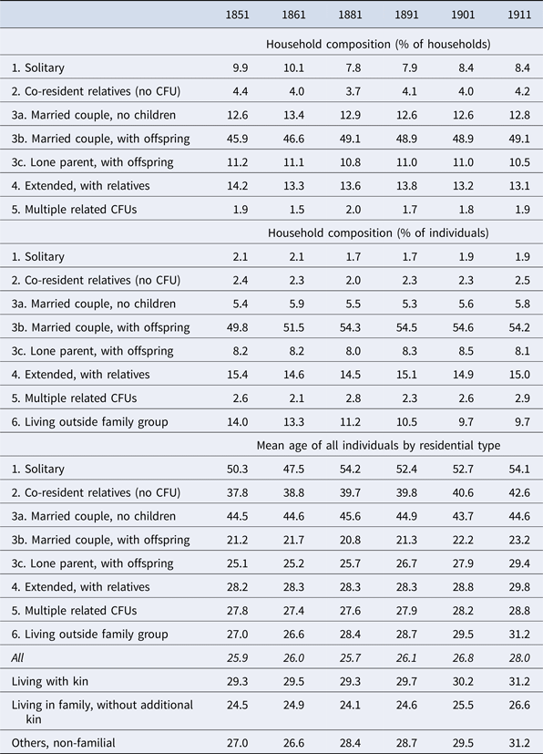
Table 4 presents a breakdown of household composition in England and Wales from 1851–1911 according to the familiar Hammel-Laslett household classification scheme. The top panel confirms that the increased proportions of solitary households does not have its roots in the second half of the nineteenth century. The proportion of solitary households remained relatively stable over the period, ranging from around 8 to 10 per cent of all households, with the period 1891–1911 actually witnessing a very small rise in the proportion of solitary households.Footnote ³⁹ However because different household types by definition vary by size, using the household as the denominator may obscure the relative importance of groups within the population as a whole.Footnote ⁴⁰ This is particularly true of solitary households, and the contrast is demonstrated by comparison with the middle panel of Table 4. This shows that the proportion of the population living in solitary households was actually small and quite insignificant for the entire period, remaining unchanged at around 2 per cent. Yet even this figure is potentially misleading from a long-term comparative perspective, since the Hammel-Laslett household classification focuses essentially on families and their co-resident relatives. Thus, in this classification scheme, solitaries (and those in other household types) could live with any number of servants, boarders and lodgers. An extreme example of this is the ‘solitary’ household of the Earl of Lonsdale, who, in 1787 was recorded as living in Lowther (Westmorland) on his own, but attended by 49 servants.Footnote ⁴¹

Table 4.

Household classification (1851–1911)

Source: I-CeM database.

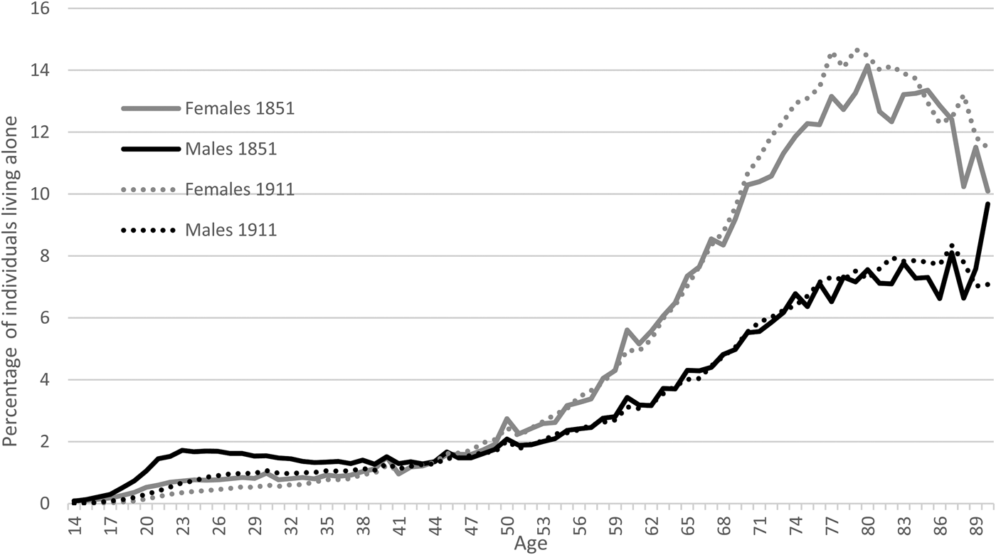
A more realistic picture of those living a solitary life is presented in Figure 2, which shows the proportion living totally alone, by age and sex, in 1851 and 1911. As in contemporary society, living alone was a feature primarily of later life. Prior to age 45, the numbers of either sex living alone were negligible. However, between 1851 and 1911 the proportions of younger people living alone actually decreased, especially in the case of men in their twenties. It was only after age 45 that the chances of living alone began to rise significantly for both men and women: rates rising quite rapidly for women, by some 2 per cent every five years, yet less so for men. In this respect, it is important to realise that due to a combination of falling levels of fertility and improved mortality, especially for females, as discussed earlier, the population of the country as a whole started to age gradually towards the end of the period under examination. As shown in the lower panel of Table 4, between 1851 and 1891 the mean age was little changed – from 25.9 to 26.1, yet thereafter it rose slowly to reach 26.8 by 1901 and 28 by 1911. Despite this slight ageing of the population, little change in the experience of living alone was witnessed between 1851 and 1911; levels of living alone peaked at around age 85 at 8 per cent for males, while for women the peak was around 14 per cent at age 80, and was slightly higher in 1911. The last was most probably as a result of the improved female mortality in the ages from approximately 55 to 80 relative to that for males, combined with the fact that women tend to marry men who are older. Women are therefore more likely to be widowed than men are. Interestingly, after age 80 – unlike men – the proportions of women living alone fell almost as rapidly as they had previously risen, suggesting that in extreme old age some women who may previously lived alone changed their residential arrangements. This characteristic now seems to be the norm for both sexes in the UK: in 2014 the proportion of males living alone decreased from 18.2 per cent for those aged 65 to 74, to 8.8 per cent for those 75 and over, while for women, the respective figures were 31.8 and 25 per cent.Footnote ⁴² Residing in an institution – primarily a workhouse – accounted for some of the age and gender differences in living alone. In 1851, 2.4 per cent of females aged 60 and over where recorded as living in an institution, compared to 4.1 per cent of men. By 1911 the respective figures were 4.1 and 7.6 per cent. So, while elderly men were more likely to be resident in institutions than women, the percentage of both men and women living in institutions increased over time despite the fact that in the population as a whole the proportion of individuals aged 65 and over living alone rose slightly between 1851 and 1911. It might be expected that the introduction of old age pensions in 1909 had an impact on the proportion of elderly living alone given their potential greater financial independence.Footnote ⁴³ From January 1909 British nationals aged 70 or over who had resided in the UK (except the Channel Island and the Isle of Man) for at least 20 years, could apply for a pension. A means test was applied (for which accommodation support from relatives counted towards income) and those who had been in receipt of poor relief in the past year, with various exceptions, were ineligible.Footnote ⁴⁴ Despite this, there was little change in the overall proportions of elderly older than 70 living in institutions between 1901 and 1911, and most of the change was accounted for by males: the percentage of women aged 70 or over in institutions being 5.7 in 1901 and 5.2 in 1911, the respective figures for elderly men being 9.5 and 8.2 per cent.Footnote ⁴⁵ Rather than creating greater independence, the proportion of those aged 70 and over living as a lone head of household (with or without servants or boarders) fell very slightly between 1901 and 1911 from 18.3 to 17.3 per cent in the case of women and 9.5 to 8.6 per cent for men. In contrast, there was a very small increase for those 70 or over living with children or other relatives, from 65.6 to 67.2 per cent for women and from 50.8 to 53.5 per cent for men between 1901 and 1911 (most of whom were daughters). These small changes in the situation of the elderly between 1901 and 1911 would seem to support the notion that in the years immediately following the introduction of old age pensions in 1909 relatively few moved from indoor relief to pension. The most likely explanations for this are the relative amounts available from the new pension scheme, and moreover, the lack of alternatives. From a survey of some 12 workhouses just prior to the Pensions Act, Edith Sellers estimated that some 45 per cent of inmates were infirm to the extent that they required continued medical support and care, a further 20 per cent had no living relative and an additional 16.5 per cent had no relative living close by.Footnote ⁴⁶ Indeed, local evidence suggests that many elderly workhouse inmates decided not to claim the new pension as they perceived themselves to be better off retaining their current arrangement, due to their medical care needs or to the lack of alternative appropriate arrangements. Workhouse boards were reluctant or powerless to force inmates to take their pension instead of staying in the institution.Footnote ⁴⁷ In short, few of the patterns in living alone presented in Figure 2 can be explained by changes in institutional living resulting from the provision of old age pensions in 1909.

Figure 2.

Percentage of population living alone: males and females (1851–1911).

Note: Includes individuals within institutions.Source: I-CeM database.

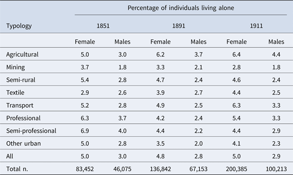
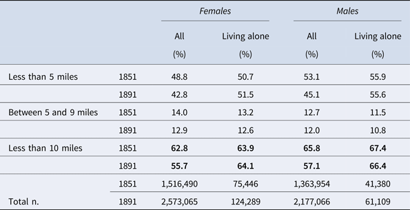
While, for the sake of brevity, the focus of this article is not on geographical variation, in relation to solitary living, Snell has commented on a significant shift in the geography of living alone in Great Britain between the nineteenth century and the present. He notes that historically higher proportions of solitary households tended to be found in rural areas and areas where low-wage rates dominated, in contrast, solitary living is today concentrated in the south and south-west of England – mainly coastal, retirement areas – as well as in large cities.Footnote ⁴⁸ Exploring this transformation further, Table 5 examines the geography of living alone by ‘typologies’. This is a classification based on Registration Sub-Districts (RSDs), into which the country was divided for the administration of the census and the registration of births, marriages and deaths. There were 2,176 RSDs in England and Wales in 1851 and 2,009 in 1911. Each RSD has been assigned to one of eight categories according to the mix of occupations observed in the RSD, together with population density, and the resulting typology for each RSD then allocated to the households within it.Footnote ⁴⁹ It should also be noted the proportion of the population living in the different typologies changes over time, so the relative population share of each typology will vary across census years. In particular, the number of RSDs classed as agricultural falls over time, as one might expect, as a result of urban growth and related rural depopulation. While the proportion of individuals living alone in the agricultural RSDs increased over time and by 1911 recorded the largest proportions of living alone, the rural/urban switch in living alone noted by Snell is perhaps not so straightforward. The situation in 1851 is one in which there is no clear distinction between those RSDs that could be classed as rural in comparison with those that might be considered urban. The distinction between the two is only evident later in the nineteenth century. One feature of note in urban areas was the relative lack of living alone in areas typified by textile working, especially in the case of women in 1851. It would be reasonable to speculate that the dislocation of families resulting from rural-urban migration flows may have caused the relative increase of living alone in agricultural areas in the late nineteenth and early twentieth centuries. As shown in Table 6, as the century progressed, fewer people were living locally as a whole – that is, born within the parish in which they resided or perhaps a neighbouring parish. In 1851 some 63 per cent of females and 66 per cent of males aged 45 and over (and both within England and Wales) lived within ten miles of their place of birth, yet by 1891 these figures had fallen to some 55 per cent and 57 per cent, respectively. Yet for those living alone, no such decline was witnessed, thus by the end of the century those living alone were, pro rata, more likely than the population as a whole to be living locally. This may be indicative that rural depopulation among the younger generations was isolating the elderly. It could also potentially indicate that elderly individuals born locally, especially those in rural areas, were able to live alone because they had kin close by or were an acknowledged part of a community that could provide support if it was needed. Being a local may also have presented individuals with greater opportunity to receive alms of varying kinds and greater access to subsidised housing.

Table 5.

Percentage of females and males aged 45 and over living alone, by type of place: 1851, 1891 and 1911

Source: I-CeM database.

Table 6.

Women and men aged 45 and over by distance from birthplace, 1851 and 1891

Note: The distances calculated in this table are straight-line ‘as the crow flies’ distances measured between the centroid of the parish of enumeration and the place of birth. Distances are only calculated for given birthplaces in England and Wales. Thus, all those recorded as being born outside of England and Wales, or with missing of incomplete birthplace information (such as giving county of birth only) are excluded from the table. The numbers excluded account from between 9 and 10 per cent in both years and for both genders. Overall, of these, roughly 1 per cent were born in Scotland, 1.6 per cent in Ireland, 0.6 per cent elsewhere overseas and 6.4 per cent recorded an incomplete or unknown birthplace. The proportions alone and living with others was roughly equal pro rata for each of these groups in both years.

Source: I-CeM database.

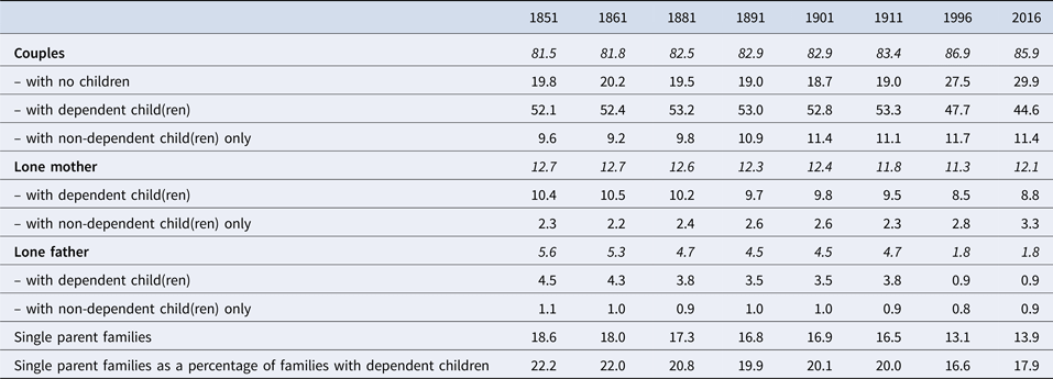
It is relevant to focus on solitary individuals and households given the increased importance of this household type over the past sixty or so years. However, historically living alone was always the experience of the minority, even among the elderly. Returning to Table 4, we can see that throughout the period 1851–1911 the nuclear family – consisting of just a single CFU with no additional family members (3a, 3b and 3c in Table 4) – was by far the most dominant household type, and increasingly so, accounting for some 70–3 per cent of all households in the period, which in turn accommodated between 63 and 69 per cent of the population. Within this, the proportion of lone-parent households (those with a head and offspring but with no spouse or additional family members) was remarkably unchanged over time, accounting for some 11 per cent of households and 8 per cent of the population. However, as shown in Table 4, the average age of individuals living in such family groups did rise over the period in question, especially between 1891 (26.7) and 1911 (29.4). This was due (as discussed in the earlier Fertility and Mortality section) to a combination of small improvements in adult mortality, especially in the case of adult women, increasingly delayed exit from the parental home, as will be discussed later, but moreover declining fertility levels from the 1870s onwards – the population was becoming older in this period primarily because there were fewer infants and very young children within the population.Footnote ⁵⁰ In recent years in the UK concern has been raised about an increase in the number of single-parent households, and in particular the number of children living in such households, linking this familial type with all manner of social ills.Footnote ⁵¹ However, estimating the number of lone-parent families (rather than households) for the contemporary period is not without difficulty. Table 7 shows that the proportion based on the evidence of the Labour Force Surveys (LFS) has changed little in the past 20 years, fluctuating generally around the 13–14 per cent mark. Yet using a combination of surveys, John Haskey has estimated that some 25 per cent of families with dependent children were headed by a single parent in 2000, up from around 1 in 7 in 1991 and 1 in 5 in 1996, noting also that ‘it is clear that it (the rate of increase) has slowed down somewhat since the late 1980s and early 1990s’.Footnote ⁵² In comparison, the proportions of single-parent families in the period 1851–1911 were higher than the official modern-day LFS-based figures, although decreasing slightly over time, from 18.6 to 16.5 per cent. The figures for 1851–1911 compare broadly with those reported for England in the three hundred years before 1851, perhaps being very slightly lower.Footnote ⁵³ The more significant change over time is not in the numbers of single parent families but the structure of lone parenthood. While declining slightly from 5.6 to 4.7, the proportion of families headed by lone fathers in the 1851–1911 period was some three times that recorded for present-day families. This key difference points to the change in the main cause of single parenthood – the switch to marriages being ended by marital dissolution rather than the death of a spouse. This also explains the low levels of lone-parent families recorded in the 20 or so years following the Second World War, a time when mortality levels in the years spanning married life had improved but divorce rates remained at low levels prior to the passing of the Divorce Reform Act of 1969. Anderson has demonstrated this point by estimating the mean duration of marriages showing that the average length of marital unions steadily declined in the four decades following 1945, by which time they reached durations similar to those estimated for the nineteenth century.Footnote ⁵⁴ Equally, the change in the gender difference between lone mothers and fathers over time will have been influenced by patterns of re-marriage. In the nineteenth century widowers were more likely to re-marry than widows, whereas in the modern era of divorce, children are more likely to be recorded as living with their mother than father, post marital dissolution.

Table 7.

Percentages of families of different types, 1851 to 1911, 1996 and 2016

Note: The figures for couples in 1996 and 2016 include opposite sex and same-sex cohabitating couples, and in 2016 civil partner couples. The percentage of recorded same-sex and civil partner couple families is, however, very small, being just 0.6 per cent of all families in 2016. Dependent children are defined in 1996 and 2016 as being never-married and aged under 16 or between 16 and 19 (under 19) and undertaking full-time education. For 1851–1911 those recorded as ‘scholars’ aged 16 to 19 are treated as dependent in order to facilitate comparison.

Source: I-CeM database; Office for National Statistics, Families and households in the UK: 2016 (London, 2016), https://www.ons.gov.uk/peoplepopulationandcommunity/birthsdeathsandmarriages/families/bulletins/familiesandhouseholds/2016

7. Co-resident kin

The subject of relatives living within the household holds a special position in the literature relating to the history of the English family. This is because it was the observed lack of co-resident relatives in two listings for the parish of Clayworth for 1676 and 1688, contained within the rector's book for that parish, which spurred Peter Laslett to embark on the research project that eventually led to the publication of Household and family in past time (HFPT) – encouraging him to challenge the then orthodox view that the small nuclear family was a comparatively recent phenomenon, resulting from capitalist-driven urban industrialisation.Footnote ⁵⁵ Laslett's famous announcement in HFPT in the form of a null hypothesis that ‘the present state of evidence forces us to assume that its [the family's] organization was always and invariably nuclear unless the contrary can be proven’Footnote ⁵⁶ threw down a gauntlet to others to either confirm or contradict this assertion.

The continued predominance of the small nuclear family was demonstrated in the previous section. However we have seen that while it was dominant it was not all pervasive, nor were all households small. Indeed, Steven Ruggles has claimed that ‘a new myth has replaced the old one’, going on to suggest that the dominance of the nuclear family in the English (and American) past has been over-stated, claiming that the ‘frequency of extended-family households increased from the preindustrial period to the late nineteenth century’.Footnote ⁵⁷ This assertion is based on a graphFootnote ⁵⁸ showing the percentage of ‘extended kin’ within households combining English and American data and the claim that they experienced similar demographic regimes. The best-fit curve for the assembled data peaks around 1880 when approximately 21 per cent of households had extended kin. However, if American data points are excluded, the English peak would be in 1871, at around 23 per cent – based on just five places or data points. This is in comparison with the pre-industrial part of the curve that shows that between 1600 and 1750 consistently around 8 per cent of households had extended kin. The inclusion of data for American places again pulls this down somewhat, and if excluded the line would rise to around the 10 per cent mark.

The fact that percentages of extended households were higher in the nineteenth century than in the small sample of parish listings worked by Laslett and his associates had previously been noted by Anderson in his contribution to the Household and family in past time volume as well as by Laslett in the same volume, although the data on which these observations were based was limited.Footnote ⁵⁹ The far more comprehensive I-CeM data confirm the higher incidence of extended family households in the second half of the nineteenth century in comparison with the relatively slender evidence for the period 1600–1750. However, it did not peak in the 1870s (nor the 1880s) and then decline rapidly as Ruggles suggests. Rather, as shown by Table 4, the proportion of extended households in England and Wales was relatively flat, declining only very slightly across the period 1851–1911, from 16 to 15 per cent. Throughout this period, female-headed households, the vast majority of which were headed by widows, were less likely to be extended than those headed by males. In 1851 14.9 per cent of households headed by women were extended against 16.4 for men. By 1911 the respective figures were 13.8 and 15.3. Moreover, given that the overall number of male heads in each census year was five or more times that of females, the overwhelming majority of extended households were headed by men – 82.7 per cent in 1851 and 83.8 per cent in 1911.

It has already been noted that due to a combination of demographic changes, the population as a whole aged slightly over the course of the last two decades covered by the I-CeM data. The bottom panel of Table 4 illustrates that this rise in average ages affected both those individuals living with kin and those not living with kin, indeed, the rise was lower for those in the former category than the latter. Between 1891 and 1911 the mean age of individuals living with kin rose slightly from 29.7 to 31.2, while the mean age of those living with nuclear family members increased from 24.6 to 26.6. Indeed, the group most affected by the slight ageing of the population was those individuals living apart from other family members altogether.

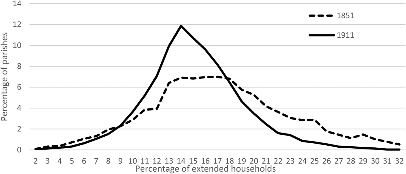
Turning to geographical variance, Figure 3 shows that the more important change in the period was not in the overall proportion of extended family households (as illustrated by Table 4) but rather the fact that the proportion of such households by place changed significantly over time. Essentially what Figure 3 illustrates is that in 1851 there were quite wide geographical variations in the incidence of extended households, with a sizable proportion of parishes experiencing quite high percentages of extended households, yet by 1911 the variance had substantially changed, with the proportion of extended households for the majority of parishes being much closer to the national mean. In effect the distribution curve of the proportion of extended households by parish for 1911 is close to a typical bell-shaped normal distribution, while in 1851 the curve was flatter and skewed to the right. This transformation appears to have taken place gradually between the two dates. Thus, over time geographical variance diminished. In 1851 half of all parishes recorded an extended household rate of 16 per cent of more; a quarter had rates of 19 per cent of more; a tenth of all parishes recorded rates upwards of 22 per cent and a twentieth had one in four or more households extended. In comparison, the respective figures in 1911 were 15, 17, 19 and 20 per cent.Footnote ⁶⁰

Figure 3.

Frequency of parishes with different percentages of extended households, 1851 and 1911.

Source: I-CeM database.

The changing shape of the curves depicted in Figure 3 may also have relevance for the interpretation of the relatively scarce household composition data for the pre-industrial period. What we know of this earlier period is based on a small number of household listings analysed primarily by Laslett and Wall. Neither would have claimed the surviving listings to be anything approaching a representative sample. However, we now know that the distribution curve of the incidence of extended households by parish in 1851, the nearest we have at a representative national level to any earlier, pre-industrial period, is not a normal shaped distribution curve. If the curve for the pre-industrial age was similar to this, or flatter still, then where the parishes for which early records survive lie on this curve becomes critically important. Given that one might reasonably expect geographic variation of household forms to be as least as great in the pre-industrial age as in 1851 – if not greater – than it would be equally reasonable to expect there to have been places experiencing much higher levels of extended households than the few surviving records and documentary evidence suggest.

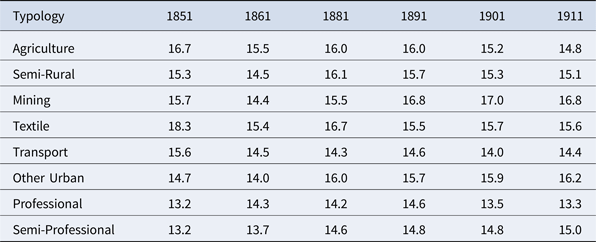
In an attempt to throw light on the nature of this shift in distribution, the situation of extended households is examined by geographical typology, as shown in Table 8. This analysis shows that agricultural areas had slightly higher proportions of extended households from 1851–1881, especially in 1851 when agriculture was at its greatest extent, accounting for two thirds of all RSDs,Footnote ⁶¹ after which the proportion of RSDs dominated by agriculture declines slightly. In contrast, the proportion of extended households in mining areas increased by a small margin. Yet what is particularly striking is that in the mid-nineteenth century, textile areas recorded the highest proportions of extended family households, while urbanised Professional and Semi-Professional areas were consistently low by comparison.

Table 8.

Percentage of extended households within each Registration Sub-District typology (1851–1911)

Source: I-CeM database.

Turning attention to individual occupation groups, continuities are revealed, but also some interesting changes. Looking first at male-headed extended households in 1851 (in which year 16.4 per cent of male-headed households were extended compared to 14.9 per cent of female-headed households), these indicate broad similarities with the data for the period 1750–1821 obtained by Wall from six rural or semi-rural communities.Footnote ⁶² In 1851, the occupations with the highest percentages of extended households were inn and hotel keepers and publicans (24.3 per cent – beer sellers were 21.2 per cent) and farmers (23.1 per cent, farm bailiffs also recorded 17.1 per cent), while other top 25 occupations included builders (21.2 per cent), grocers (19 per cent), confectioners (18.9 per cent), as well as bakers, wheelwrights and greengrocers (16.8–16.9 per cent), all of which could be typified as ‘family’ businesses.Footnote ⁶³ However, the top 25 individual occupations also included cotton weavers (20 per cent), cotton spinners (17.9 per cent), wool weavers (17.5 per cent), wool carders and combers (17.4 per cent) and general weavers (17.2 per cent), together with hosiers (18.3 per cent). Earthenware manufacturer households also recorded high levels of extension (17.9 per cent).Footnote ⁶⁴ Those occupations with the lowest levels of extended households – ranging between 12.7–10.5 per cent – include a range of service-orientated occupations such as coachmen, grooms, stablemen, as well as railway porters and labourers, and police, whose ability to offer accommodation to relatives might have been constrained because their employer may have provided and controlled their housing. Further, working-class occupations with low levels of extended households included general labourers (14 per cent), plasterers (14 per cent), messengers and watchmen (12.8 per cent), bricklayer's labourers (13.3 per cent) and hawkers (13.6 per cent). Households headed by agricultural labourers, the most numerous of all household types, were in the middle of the distribution (15.6 per cent). However, by 1911, while inn keepers and publicans, beer sellers and farmers still held the top three positions (at 20–2 per cent) and family-orientated occupations such as greengrocers, confectioners, builders and bakers each held their own, the top 30 individual occupations for household extension now included a number of traditional working-class occupations – including chimney sweeps, coal miners (above and below ground), road labourers, town drainage and sewerage workers, harbourmen and bargemen. Interestingly, cotton and wool workers had fallen out of the top ranked occupations with extended households, but earthenware workers remained. At the other end of the spectrum, as might be expected, were again a number of service-related occupations, together with police, and now also soldiers (8.9 per cent),Footnote ⁶⁵ but these were joined by a number of higher social status occupations: bankers (13.1 per cent), bank officials (12.5 per cent), physicians (12 per cent), solicitors (10.8 per cent), and lowest of all except the service occupations, clergymen (10.7 per cent). While shifts in the proportion of extended households between occupation groups can be observed over time, it is also clearly the case that extended households can be found across all occupational groups in the period under study.

Large numbers of the females heading extended family households recorded no occupation at all – 46 per cent in 1851, rising to 63 per cent by 1911 – in part a feature of the fact that a large percentage of females heads were aged 65 or over. Those who did record an occupation – current or previous – exhibited a number of characteristics similar to their male counterparts. At both the start and the end of the period the households of those recorded as farmers and inn keepers were more likely to be extended – with levels of generally around 24 per cent – than those of women in other occupations. The households of tradeswomen also record a relatively high percentage of extended households (1851: bakers, 21.9 per cent; grocers, 16 per cent; 1911: greengrocers, 21.9 per cent; butchers, 20.1 per cent; grocers, 17.2 per cent) over the period, but generally the households of women who recorded an occupation were less likely to be extended that those of their male counterparts.

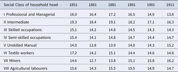
The variations over time in extended households by ‘typology’ are, in part, confirmed by Table 9, which displays proportions of extended households by the social class of the household head.Footnote ⁶⁶ This confirms that textile workers in 1851 experienced high levels of extended households and that levels declined thereafter, while the figures for miners rose throughout the period. Social class II consistently recorded the highest proportion of extended households. This class not only includes farmers but also most of the tradesmen and dealers, such as bakers, shopkeepers and innkeepers. The professional and managerial household heads of social class I (in contrast to the classification by RSD typology) show the lowest counts of extended households only towards the end of the period in question, while at the other end of the social spectrum the unskilled workers of social class V consistently record the lowest proportion of extended households in the period 1851–1891, but then, like miners, display an increase.

Table 9.

Percentage of extended households by social class of household head (1851–1911)

Source: I-CeM database.

Thus, while there was relatively little change in the overall proportion of households with extended co-resident relatives nationally over the period 1851–1911, this masks previously hidden structural change. Setting aside farmers, tradesmen and shopkeepers, the period in question was one that witnessed the households of the working class become, pro rata, more likely to be extended, and those in professional occupation less likely. As discussed in the earlier section commenting on the situation of living alone, changes in institutional care and the introduction of old age pensions in 1909 did not result in any significant shifts in patterns of familial co-residence. Rather these may have been an artefact of demographic changes: declines in fertility in the professional classes may have also limited married children living with parents, while improved mortality among working-class families may have increased the ability of generations to co-reside. To an extent, this would also fit with the experience of those living in textile-dominated areas, who witnessed a rapid and sharp decline in their total marital fertility rates from 1881, yet would not explain the experience of miners’ households, which – while falling – recorded the highest levels of fertility of all occupations throughout the period.Footnote ⁶⁷ However, before exploring these changing relationships further, it is important to consider who these extended kin were.

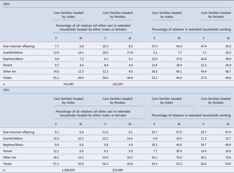
So who were these extended kin? Curiously, given the attention accorded to extended households, this question seems to have been seldom addressed. Anderson, in his Continuity and Change article states that in 1851 most co-residing relatives were drawn from a narrow band of close kin – mainly ever-married children, grandchildren, parents, siblings, nieces and nephews – suggesting that, as for the pre-1851 period, most were young individuals separated from their own families either by death or work.Footnote ⁶⁸ However, co-resident relatives are not quite the same as extended kin. Following the standard definition of an extended household, the extension is from the core CFU and how this is defined will depend on the assignment of headship. Thus, for example, if an extended household comprised a head plus married daughter, son-in-law and grandchild, it is the head who should be treated as the extension to main family, not the son-in-law and grandchild.Footnote ⁶⁹ Applying these rules, Table 10 identifies those who formed the extension to the principal family. This illustrates that extended kin were slightly more likely to be female – more so by the end of the period. Grandchildren formed the largest group, and pro rata were more numerous in female-headed households than males, yet diminished in importance over time in both male- and female-headed households, probably due to improvements in mortality with fewer children being rendered ‘parentless’ at young ages. Applying the definition of extension as used in the definition of extended households reveals that those banded together under the ‘other kin’ heading – the majority of whom were females – were more important in terms of extension than ever-married sons and daughters. This runs contrary to the suggestion made earlier by Anderson. Many of these were siblings of the head, yet also included in their number were a wide spectrum of aunts, uncles, cousins and even grandparents. Moreover, over time, this group increased in relative importance in both male- and female-headed households, especially in the case of female ‘other kin’ in households headed by males. This may be a feature of changing demography, with sisters marrying later or not at all being more prone to join the household of their brother towards the end of the period.Footnote ⁷⁰ Ever-married daughters were more likely to be present than sons in both male- and female-headed extended families, proportionally more so in the case of the latter. While male-headed extended families tended to outnumber those headed by a female by some 4.5:1, in the case of the latter both grandchildren and ever-married sons and daughters can be seen to form a larger element of the extended group of relatives in comparison to male-headed extended families. In this regard, male-headed extended families can be seen to have been more varied in their composition, incorporating a broader range of relatives than female-headed extended families, however, this diversity diminished over time.

Table 10.

Extended family members by sex of household head and if working, 1851 and 1911.

Note: See text for definition of extended family members. This table counts just the extended family members, not the core CFU from which they are extended. For the small number of households that are multiple in type and contain two of more CFUs (between 1.5–2 per cent in each census year, see Table 4), the first CFU is taken as the core family, as per the Hammel-Laslett household classification scheme.

Source: I-CeM database.

The right hand side of Table 10 indicates which of the extended kin group were recorded as working with an occupation and which were not. Perhaps not surprisingly, males in the extended group were more likely to be recorded as working than females, but only the proportions of men in employment increased significantly over time, the proportion of females working remaining at around a quarter in both male- and female-headed households. Where married sons (and sons-in-law) co-resided as an extension to the core family, they were nearly always working, but increasingly so were nephews, ‘other kin’ (largely brothers) and even fathers. In the case of working women, nieces, while less important numerically, overtook ever-married daughters in the extended kin group in terms of contributing to the household budget by the end of the period,Footnote ⁷¹ and other female kin were important too as workers, especially in male-headed extended households by 1911.

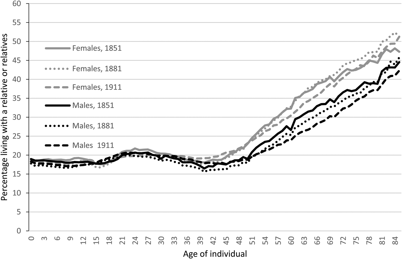
In general terms, the presence of an extended co-resident kin group can be seen as one generation supplementing or supporting another. This is illustrated in outline via Figure 4, which shows the proportions of those living with a relative by age (in essence all co-resident kin living in extended or multiple type households, not extended kin per se). The pattern is virtually the same for both sexes and unchanged over time for those aged under 40. From birth up until the age of around 20 the proportion of individuals living with a relative largely fluctuated around the 17–18 per cent level. Thereafter the levels rose slightly to reach a mini peak at around age 25 with levels of around 20–1 per cent. Then they fell back to a slightly broader range of between 15.5–19 per cent at age 40. From this age the percentage living with relatives rose steadily, yet at different rates for males compared to females. By age 50 the difference between males and females was around 4–5 per cent (M 18–9 per cent; F 23 per cent). In 1851 this gender difference remained at around 5 to 6 percentage points at subsequent ages being around 32 and 27 per cent respectively for females and males at age 50, 39 and 34 per cent at age 70 and 44 and 39 per cent at age 80. Yet by 1911 the overall levels of those in later life co-residing with relatives had declined and the gender differential had increased – the levels for females and males respectively being 30 and 24 at age 60; 38 and 30 at age 70 and 45.5 and 37 at age 80. Although it is impossible to say with certainty what may have caused the relative rise in the proportions of kin working within the household shown in Table 10, it may have been due to a shift in the balance of extended households from being more supportive (providing support to the extension) in the earlier period, to being increasingly supporting (receiving support from the extension) in the latter period. This is consistent with the increased likelihood of extended households being working class as the period progressed.

Figure 4.

Percentages of males and females living with a relative, by age: 1851, 1881 and 1911.

Note: A relative is defined as any co-resident kin member who is not in an individual's own CFU. Thus, in an extended household all the co-resident kin are in effect viewed as living with a relative. For example, in a household headed by a widowed mother living together with her son and his wife, the mother is the relative of both the son and his wife as she is an extension to their CFU, while, reciprocally, they are relatives to the mother.Source: I-CeM database.

These significant temporal shifts in the structure of the extended family household require further analysis beyond this general overview of the period. However, it is important to relate these new findings to previous work on nineteenth-century households. In his classic study of the cotton manufacturing mill town of Preston in 1851, Anderson observed what can now be seen as high levels of households with co-resident relatives, some 23 per cent.Footnote ⁷² While this is consistent with the high proportions of extended households experienced by textile workers in 1851 as demonstrated earlier, it also suggests that the example of Preston was more of an exception than the norm.Footnote ⁷³ In explaining the presence of co-residing relatives Anderson suggested that this may be accounted for by relatives helping to mind and look after young children in order to allow their mother to undertake factory work.Footnote ⁷⁴ Likewise, Eilidh Garrett has pointed to a similar residential arrangement for the woollen mill town of Keighley on the other side of the Pennines, where the availability of work for (married) women was also an important factor.Footnote ⁷⁵ The fact that the rapid and sharp declines in marital fertility experienced in textile areas from the 1880s onwards is mirrored by a decreasing importance in extended family households in these areas may not be coincidental. Linked to this, it is interesting to note that of those women working in textile-related occupations in 1851, 29.5 per cent were married, of whom 69.6 per cent had one or more co-resident offspring. By 1901 the proportion of female textile workers who were married had dropped to 17.7 per cent, of whom 60.5 per cent had a never-married child living with them. In 1911 the figures remained similar to those of 1901, being 21 and 59.5 per cent respectively. Overall, in 1851 married women with co-resident offspring accounted for 20 per cent of the female labour force in textiles, by 1911 this had reduced to 12.4 per cent.

It has also been suggested that extended household arrangements and co-residence were largely the result of conditions of extremis – usually of a short- to medium-term nature during which the household in question was experiencing a situation that required or could offer support. These were varied in nature and cause: accommodating family members newly migrant to a rapidly growing industrial town; receiving an extra wage earner or pair of hands in a time of crisis, such as sickness or bereavement; supporting newly-weds or childbirth – all in the context of the New Poor Law. The I-CeM data suggest that while there is some limited support for the notion of migrants being supported by kin in that greater proportions of extended family members were non-local than their fellow household members, the difference between the two groups was slight. Perhaps ironically, given the original proposal is mainly based on 1851 data, the difference is greater in later nineteenth and early twentieth centuries than the mid-nineteenth century.Footnote ⁷⁶ Yet the main enigma about the otherwise compelling extremis theory is why this should apparently apply to textile workers at the beginning of our period but apparently not to the bulk of the working class in social class V, who recorded the lowest levels of household extension for much of the nineteenth century, and whom one might expect to be most vulnerable and at risk of domestic instability caused by unemployment (or underemployment), sickness or mortality. However, an answer to this conundrum may lie not in vulnerability per se but in the switch from the supportive nature of kin in the earlier period, to a more supporting role in the latter period.Footnote ⁷⁷ Equally, the nature of married mothers in textile-related occupations, especially in the mid-nineteenth century, made textile communities the exception rather than the norm in many instances.

8. The position of children and residence pre-marriage

Children in all societies and at all times need the support of others. Historically, as now, this has invariably been provided by parents or a parent. However, due to one or other parent dying, in 1851 the proportion of children, boys and girls, living with both parents never reached higher than 87 per cent (Figure 5a). At that time only around three quarters of all children aged ten were living with both of their parents. As the mortality statistics presented earlier indicate, females experienced a more favourable and improving mortality situation than their male counterparts. Yet the age-specific mortality differences between males and females were such that it was not until the twentieth century that children aged 15 and under were more likely to experience the death of their father than their mother.Footnote ⁷⁸ However, the 1851 census data indicate that the proportion of children (both boys and girls) living only with their mothers rose from just over 5 to 10 per cent between birth and age ten, while those living only with their fathers rose from some 2 to 5 per cent. In the absence of mortality as an explanatory factor, differential patterns of residence following widowhood and re-marriage is the most likely explanation of this difference, with young children staying with a widowed mother, but not necessarily a widowed father. In this regard it is also noticeable that the proportions of children under the age of 16 living with a relative (but not a parent) was slightly higher than those living with a widowed father.Footnote ⁷⁹ This would point to a significant number of young children being placed with relatives in the event of their mother dying, rather than staying with their widowed father.Footnote ⁸⁰ Comparisons with Figures 5b (1881) and 5c (1911), suggest that this practice did not diminish with time, but if anything, increased slightly. From Figures 5a–c it can also be seen that a small but important proportion of the young lived without the support of either their parents or their wider family. This was more so for boys than girls, especially for boys in their teens, with the trend increasing from 1851 to the 1880s and 1890s before declining. In interpreting these trends it is important to stress that these are not all children living in workhouses, as the data in Figures 5a–c (due to the relatively small proportions) aggregate together all those in what might best be labelled as institutional care. Such establishments include not only workhouses, but also orphanages, schools, hospitals, borstals and large boarding and lodging establishments. In I-CeM it is difficult to distinguish between them since most were enumerated by the census authorities in special institutional books and cannot easily be differentiated within the data – separate institutions can be identified, but there is no standard descriptor which defines which type of institution is which.

Figure 5a.

Percentages of girls and boys with different residential arrangements by age, 1851.

Source: I-CeM database.

Figure 5b.

Percentages of girls and boys with different residential arrangements by age, 1881.

Source: I-CeM database.

Figure 5c.

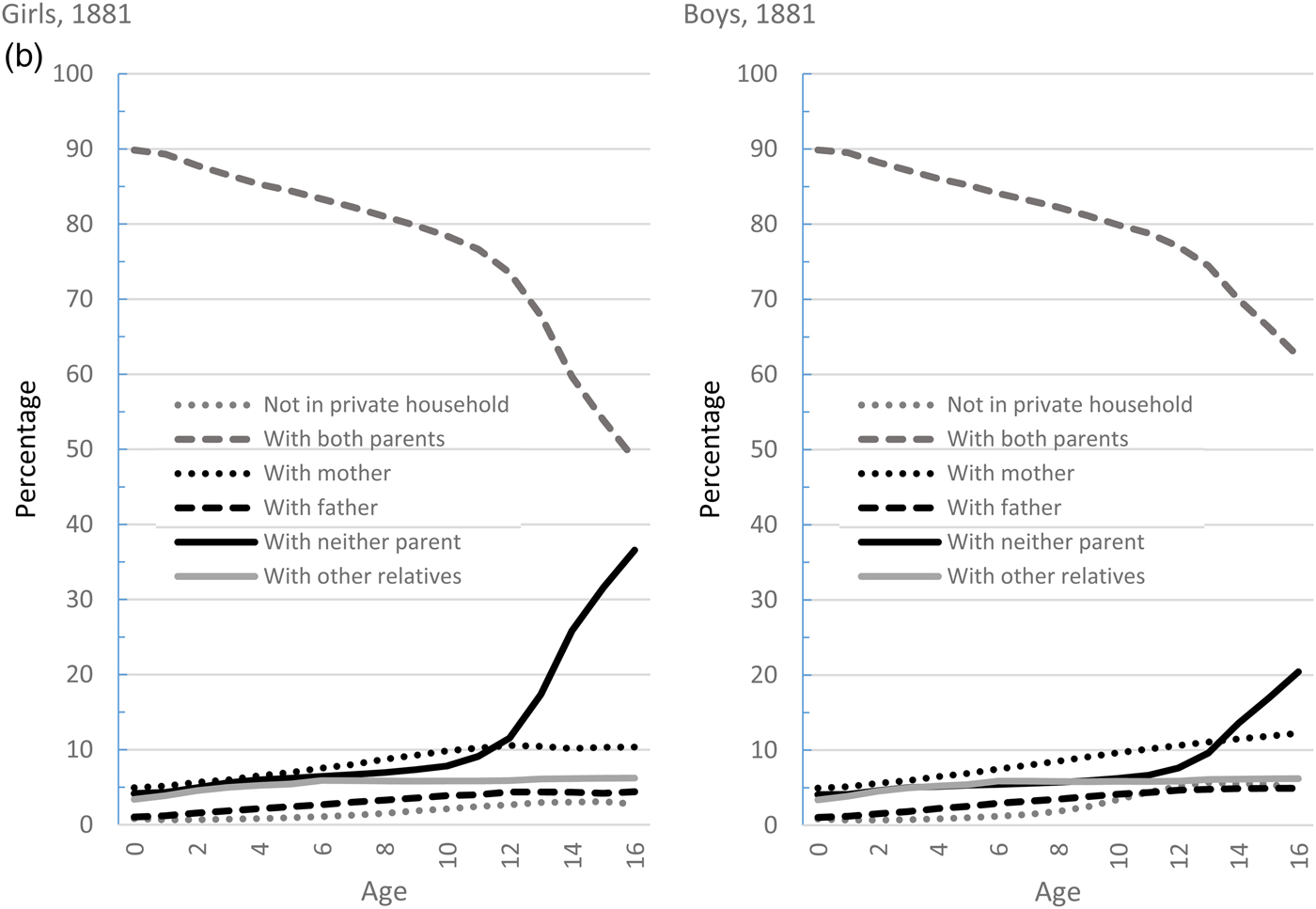
Percentages of girls and boys with different residential arrangements by age, 1911.

Source: I-CeM database.

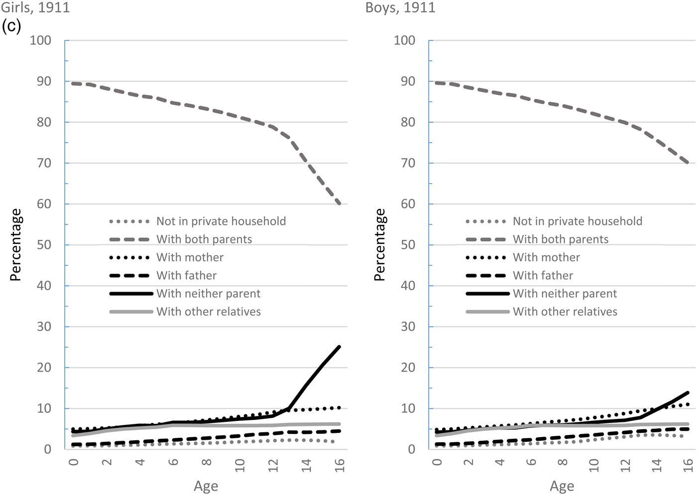
Comparing all three Figures 5a–c also demonstrates the impact of improving mortality on the family life of the young. By 1881 the proportion of boys and girls living with both parents at age ten had risen to just under 80 per cent and by 1911 was up to 82 (from 74) per cent in 1851. This progressive improvement in parental mortality and its impact on the living arrangements of young children in the period 1851–1911 can also be seen in Figure 6, which shows the proportions living with neither parent for all available census years. For those aged under ten, Figure 6 shows for boys and girls, that the curves move gradually downwards over time. This is essentially a mortality effect with greater proportions of young children living with both parents moving from 1851–1911. However, of course, parental death is not the only reason why children may not have been living with their parents. As indicated above, a few – boys more than girls – were sent away to schools, but rarely before the age of ten.Footnote ⁸¹ Young children may also have been sent to live with relatives, maybe at times when the mother was working (as may have been the case in textile towns) or equally following the birth of a new addition to the family or an illness in the family. Such relocations may have been of a short-lived and temporary nature. However, for most, the key break from the parental home came as a result of leaving home. The pace of leaving home is indicated by the slope of the respective lines in Figure 6 showing the proportion of males and females not living with either parent. From this the general trend is clear. Departure from the parental home was later for boys than girls, and became progressively later for both sexes between 1851 and 1911, even though by 1851 the age of leaving home was significantly later than in the eighteenth and early nineteenth centuries.Footnote ⁸² This general trend in the course of leaving the parental home is measured in Table 11, which shows that the singulate mean age of leaving the parental home (SMAL) rose by over two years for males between 1851 and 1911, from 18.9 to reach 21.2 by 1911.Footnote ⁸³ While leaving home for females was invariably a year to two years earlier than that of their brothers, the trend for females was similar to that of males, with female age at leaving the parental home also gradually rising by some two years from 17.6 in 1851 to reach 19.7 by 1911. These figures are, of course, average ages and, like any singulate mean, are produced on period rather than cohort numbers. It is therefore instructive to look also at what might be called the ‘take-off’ age, or the age at which the rate of leaving home started to change rapidly. In essence, with reference to the lines of the graphs presented in Figure 6, it is trying to measure the point at which the trajectory of the various lines shown switched from being a gradual (scarcely more than horizontal) rise to rising rapidly (and virtually vertically). Estimates of the ages at which this transition took place are also given in Table 11. These, together with the graphs in Figure 6, suggest that while the age of leaving home for girls became gradually later over the period, the process of leaving started early for girls. Even by 1911 girls started to leave home at 13 or 14, younger still in the nineteenth century, most usually destined for work in service of one kind or another. In contrast, for their brothers, departure from home was usually later and also a more gradual process for those under 16, and becoming more so over time.

Figure 6.

Percentages of males and females living without either parent (1851–1911).

Note: The six lines on each graph run progressively from 1851, 1861, 1881, 1891, 1901 and 1911 left to right.Source: I-CeM database.

Table 11.

Age at leaving the parental home: males and females (1851–1911)

Note: The start of the leaving home process, or ‘take-off’ age, is calculated as the age (x) at which the increase in the proportion not living with both parents between age x and x + 1 is 3 or more percent, and the difference between age x + 1 and x + 2 is 4 or more percent.

Source: I-CeM database.

Table 12.

Singulate mean number of years spent between leaving parental home and marriage: males and females (1851–1911)

Source: I-CeM database.

One of the most significant effects of the delay in leaving home and changes in the process of leaving home, was that the number of years adolescent children and young men and women spent apart from their parents and family home prior to establishing a home of their own diminished. This is shown visually by Figure 7, which contrasts the experience of living with parents with that of living with a spouse, for those aged under 35. For both males and females, the gap between the lines narrows over time, indicating that for many, the time spent between living with one's parent(s), leaving home and subsequent marriage and starting a new home was narrowing – a trend that had most likely been taking place since the late eighteenth century, or earlier.Footnote ⁸⁴ An attempt to measure the extent of this process is provided in Table 12, which gives the singulate mean number of years spent between leaving the parental home and marriage. Given that this figure calculates the difference between two period measures for events that happen at different stages of the life cycle (being calculated from the difference between SMAM and SMAL by age) it is not a measure of ‘true’ experience, and with age at leaving home in the period being delayed, it will invariably underestimate the real time spent between leaving home and marriage. Thus, a girl leaving for service at the age of 12 in 1851, would in all probability not marry before the age of 23 in 1872, maybe later, giving rise to a gap between the two events of 11 years or more. Yet despite this problem, the figures are still indicative of the broader trends over time. In outline, the gap was nearly always greater for females than males, yet at the start of the period was the same for both sexes.Footnote ⁸⁵ Over time the duration of the average gap between leaving home and marriage shortened slightly faster for men in relation to women, especially in the third quarter of the century. Thus, while the rise in the age at marriage over the period 1851–1911 was largely mirrored by later departure from the parental home, the latter out-paced the former, slightly more so for boys than girls, for whom service, although declining, remained an important employment pre-marriage (see Table 3, which shows the mean number of servants per household drop from 0.3 in 1851, to 0.21 by 1891 and 0.16 by 1911). Overall, the time spent apart from family prior to marriage was reduced and while the social consequences of this are difficult to determine, such a shift may have been influential in the dramatic decline of illegitimate fertility rates, which coincided with this change.Footnote ⁸⁶ The combined effect of the processes of leaving home and of onset of marriage is depicted in Figure 8, which captures the changing experience of those in their teens and early twenties. The percentage living away from family, either parent(s) or other relatives, at these ages dropped significantly after 1851, especially in the early years of the twentieth century. For males, the percentage living apart from their family and relatives at age 20 was halved between 1851 and 1911, dropping from 34 to 17 per cent. For females, the decline at age 20 was not as marked, being around a third, but still important – from 37 to 27 per cent – and matched by a similar decline at age 15, from 25 to 14 per cent. Yet the biggest change in experience, perhaps one of the most important changes in terms of family life in the period, was those in their earlier teens who – as a result of decreased employment, increased schooling, delayed departure from the family home, and, in part, increased survival of their parents – remained part of the family of their childhood for longer.Footnote ⁸⁷

Figure 7.

Percentages of males and females living apart from a parent and living with a spouse, 1851 and 1911.

Source: I-CeM database.

Figure 8.

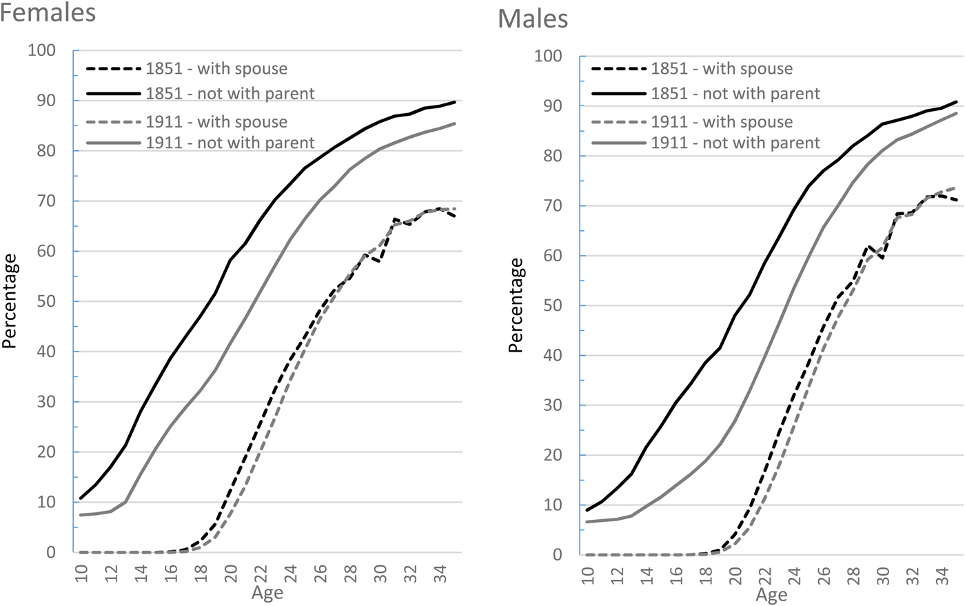
Percentages of males and females living separate from other family members: 1851, 1891 and 1911.

Source: I-CeM database.