




1. Introduction
This article has been prepared in recognition of Mark Ablowitz’s 80th birthday. It is inspired by his works establishing important connections between nonlinear waves, integrable systems and functions of a complex variable. Although it is not about waves and integrable systems per se, it presents new connections between analytic functions and numerical methods (especially for quadrature and differentiation). These computational tools can be used in a variety of settings, with nonlinear wave models a promising direction that mostly remains to be explored.
Formulas for derivative approximations and for numerical quadrature that are specific to analytic functions in the complex plane can be far more effective than traditional formulas that do not utilize these properties. Some of these are described in Sections 2 and 3, respectively. This is followed in Section 4 with a discussion of some features that generalize from the 2-D complex plane to harmonic functions in higher dimensions (motivated by us living in a 3-D world, and with many physical field variables satisfying the 3-D Laplace equation). The last section contains some concluding remarks.
The next three subsections of this Introduction contain some brief remarks on traditional aspects of Finite Differences (FD), the Trapezoidal Rule (TR) and the Euler–Maclaurin (EML) formula.
1.1. Finite differences
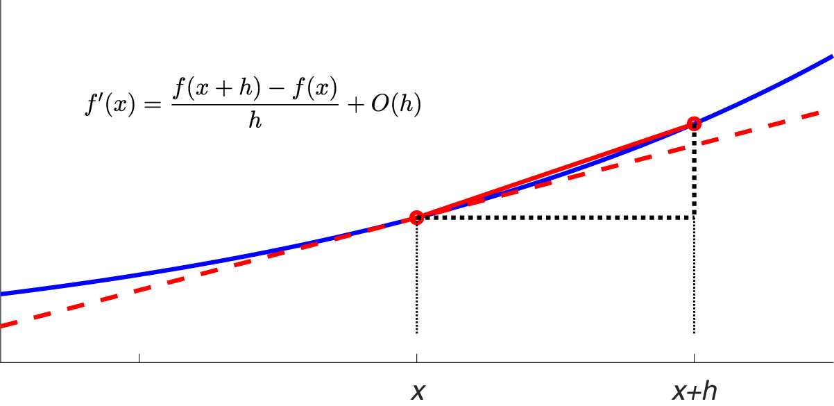
The first use of FD formulas is usually attributed to Jost Bürgi around 1592, in the contexts of interpolation and creating trigonometric tables. The classical definition of the first derivative is illustrated in Figure 1. With the step length  $h$ small but not infinitesimal, it amounts to a very simple case of a finite difference (FD) formula. The first order accuracy of this approximation (local error
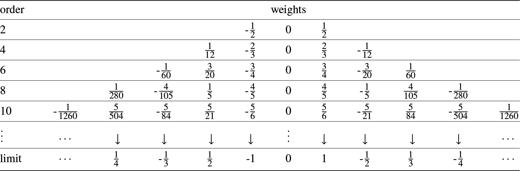
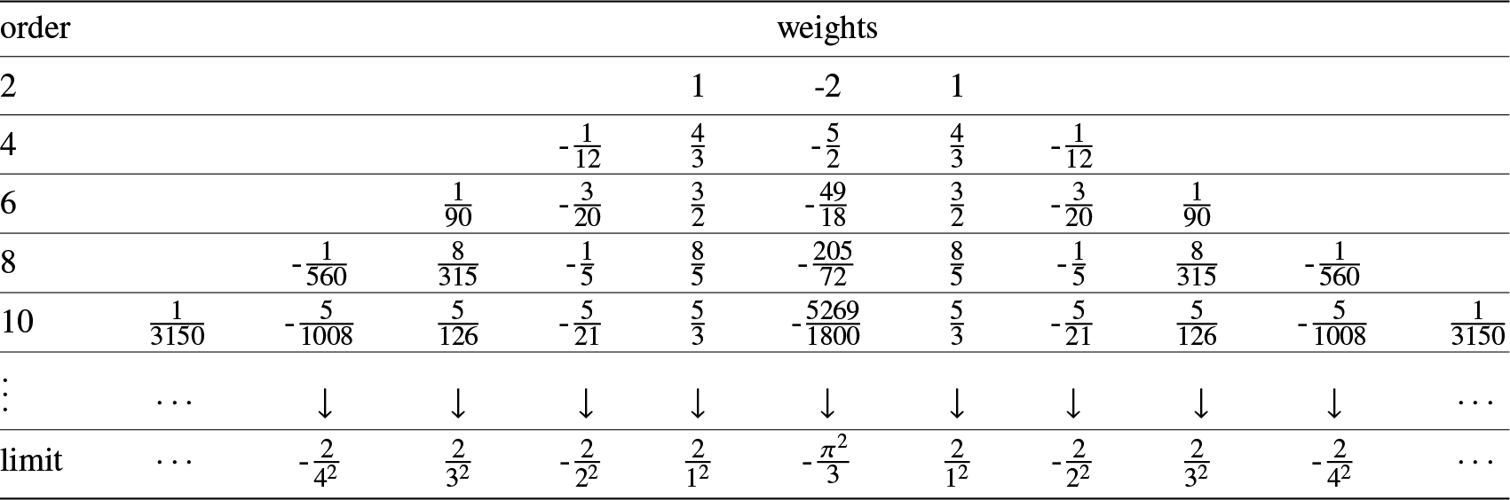
 $O(h^{1})$) makes it grossly inefficient in almost all cases. FD formulas of higher orders of accuracy are generally far more effective. Some centred approximations are illustrated in Tables 1 and 2. A striking feature in these tables is that each column converges to a well-defined limit. With
 $k$ denoting the distance of a node to the stencil centre, weights for odd-order derivatives decay as
 $O(1/k)$ and for even order derivatives as
 $O(1/k^{2})$. Both decay rates are problematically slow, as a derivative is a completely local property of a function, and should not be strongly dependent on distant features. For one-sided stencils, the situation is much worse still, with some weights diverging exponentially with the accuracy order of the approximation.
Weights for centred FD approximations to the first derivative on a grid with spacing h (omitting the factor 1 ${/}$h)

Table 1 Long description
The table lists coefficient sets for centered finite-difference approximations of the first derivative on an evenly spaced grid, with the overall scaling by the grid spacing omitted. Each row gives the weights for a chosen accuracy order, arranged symmetrically around the center point. For second order, three points are used with negative weight on the left, zero at the center, and positive weight on the right. As the order increases to fourth, sixth, eighth, and tenth, the stencil widens to five, seven, nine, and eleven points, respectively, while keeping a zero center weight and opposite-sign pairs at equal distances. The largest magnitudes occur at the nearest neighbors to the center, and the weights decrease in magnitude as points move farther away. Signs alternate as you move outward from the center, reflecting cancellation that improves accuracy. The final row indicates a limiting pattern for an infinitely wide stencil, where weights continue outward with decreasing magnitude. Values are coefficients only; to obtain the derivative approximation they must be combined with sampled function values and then scaled by the reciprocal of the grid spacing.
1.2. The trapezoidal rule
With equi-spaced nodes  $x_{k}=x_{0}+kh$,
 $k=0,1,\ldots,n$, the trapezoidal rule (TR) can be written as
 \begin{equation}
\int_{x_{0}}^{\,x_{n}}f(x)dx=h\left\{\frac{1}{2}f(x_{0})+1\cdot f(x_{1})+1\cdot f(x_{2})+\ldots+1\cdot f(x_{n-1})+\frac{1}{2}f(x_{n})\right\} +O(h^{2}),
\end{equation}
A simple FD formula, serving when  $h\rightarrow0$ as a definition of the first derivative.

Weights for centred FD approximations to the second derivative (omitting the factor  $1{/}$h2)

Table 2 Long description
The table lists coefficient sets used in centered finite-difference approximations of a second derivative, with a common scaling factor omitted. Each row gives the weights for a chosen accuracy order, arranged from left offsets through the center point to right offsets, and the pattern is symmetric about the center. For second order, the three-point stencil uses weights one, negative two, one. For fourth order, a five-point stencil adds small negative outer weights and larger positive inner weights, with a more negative center weight than the second-order case. For sixth, eighth, and tenth order, the stencil expands to seven, nine, and eleven points, respectively, with alternating signs as you move outward and with magnitudes decreasing toward the farthest points. Across increasing order, the center coefficient becomes increasingly negative while the nearest-neighbor positive weights increase, reflecting a sharper central curvature estimate balanced by more surrounding points. The final “limit” row indicates the trend as order grows: weights follow an alternating pattern that decays with distance from the center, while the center approaches a fixed negative constant. Values are presented as exact fractions, and because the common scaling factor is omitted, the numbers must be combined with the appropriate grid-spacing factor when used in calculations.
or more schematically as
 \begin{equation}
\int f(x)dx=h\left\{\frac{1}{2}\quad1\quad1\quad1\;\ldots\;1\quad\frac{1}{2}\right\} f+O(h^{2}).
\end{equation}
Babylonian astronomers used this approximation already around 50 BC, noting the subtlety of halving the first and last entries [Reference Ossendrijver10]. As in the case of FD approximations, computational effectiveness requires the accuracy order to be considerably higher. Modern textbooks usually focus on the Simpson and Newton-Cotes enhancements. In the notation of (2), the former can be summarized as
 \begin{equation}
\int f(x)dx=\frac{h}{3}\left\{1\quad4\quad2\quad4\;\ldots\;4\quad1\right\} f+O(h^{4}),
\end{equation}
typically derived by fitting parabolas to nodes  $\left\{x_{0},x_{1},x_{2}\right\} ,\;\left\{x_{2},x_{3},x_{4}\right\} ,\ldots$ and integrating these exactly. This formula was written down by Simpson in 1715 based on posthumous notes by Newton. The method was however used long before by Kepler (1571-1630) for the non-astronomical task of estimating volumes of wine barrels. The Newton-Cotes (NC) sequence of methods uses similarly piecewise cubics, quartics, etc. This is conceptually severely flawed for several reasons, including
(1) Essentially all errors in the TR come from the ends (cf., Section 1.3); one should do corrections there and not ‘contaminate’ throughout the entire interior of the interval,
(2) For periodic problems (and with smooth functions), Simpson gives roughly half the number of correct digits compared to TR; next NC method gives only one third, etc. This can be seen as follows: There are for periodic analytic functions no boundary effects and
 $\textrm{TR}(h)$ becomes spectrally accurate, with error
$O(e^{-c/h})$,
$c$ constant [Reference Trefethen and Weideman12]. The accuracy loss for Simpson’s approximation
$S(h)$ then follows from writing it as
$S(h)=\frac{1}{3}(4\:\textrm{TR}(h)-\textrm{TR}(2h))$. The results for higher order NC methods follow similarly.
(3) The NC methods become very unstable for increasing accuracy orders, with weights of large magnitude and alternating signs.


A much better follow-up to the TR was given by James Gregory already in 1670, and is described in more detail in Section 3.1. Gregory was a Scottish astronomer and mathematician (1638-1675). He described his quadrature method well over decade before Leibniz and Newton first described calculus (in 1684 and 1687, respectively). Gregory is well remembered in the astronomical community (as a telescope designer), but is mostly forgotten among mathematicians [Reference Fornberg6].
1.3. The Euler–Maclaurin formula
Around 1640, L. Euler and C. Maclaurin independently discovered the following asymptotic error expansion for the TR:
 \begin{align}
\int_{x_{0}}^{\:x_{n}} & \sim h\left\{f(x_{0})+f(x_{1})+f(x_{2})+\ldots+f(x_{n})\right\} \nonumber \\
& \quad-\;\;\frac{h}{2}\;\;\;\;\;\left\{f(x_{0})+f(x_{n})\right\} \nonumber \\
& \quad+\;\frac{h^{2}}{12}\;\:\;\;\left\{f^{(1)}(x_{0})-f^{(1)}(x_{n})\right\}\nonumber\\
& \quad-\:\frac{h^{4}}{720}\;\;\left\{f^{(3)}(x_{0})-f^{(3)}(x_{n})\right\} \nonumber \\
& \quad+\frac{h^{6}}{30240}\left\{f^{(5)}(x_{0})-f^{(5)}(x_{n})\right\} +\ldots
\end{align}
When truncated and with  $h\rightarrow0$, the error will be dominated by the first omitted term. The top two lines provide the TR. The subsequent lines show how its formal order of accuracy can be improved to any level by end corrections only. The coefficients are expressible in terms of Bernoulli numbers, with several derivations given in appendix A of [Reference Fornberg1].
2. FD formulas in the complex plane
Analytic functions form a very important special case of functions defined over a 2-D  $x,y$-plane. A function
 $f(z)$ with
 $z=x+iy$ is said to be analytic if
 $\frac{df}{dz}=\lim_{\triangle z\rightarrow0}\frac{f(z+\triangle z)-f(z)}{\triangle z}$ is uniquely defined, no matter from which direction in the complex plane
 $\triangle z$ approaches zero. One immediate consequence is that one need not distinguish
 $\frac{\partial f}{\partial x}$ from
 $\frac{\partial f}{\partial y}$ (apart from by a factor of
 $i$). Another one is that, separating
 $f(z)$ into real and imaginary parts
 \begin{equation}
f(z)=u(x,y)+i\:v(x,y),
\end{equation}
these parts will satisfy the Cauchy-Riemann (CR) equations
 \begin{equation}
\frac{\partial u}{\partial x}=\frac{\partial v}{\partial y},\qquad\frac{\partial u}{\partial y}=-\frac{\partial v}{\partial x}.
\end{equation}
Any function  $f(x)$ that possesses a Taylor expansion at some
 $x$-location can be extended to an analytic function, with a vast range of further consequences. Advantages in FD contexts include:
(1) A derivative
$f^{(k)}(z_{0})$ depends equally much on data from all directions surrounding
$z_{0}$, i.e., stencils need not extend far out just along a single line, but can surround the point
$z_{0}$.(2) The CR equations (6) strongly limit the range of functions these formulas need to be accurate for (compared to all smooth functions of two variables).


Let  $L$ be a linear operator that we wish to approximate at some point (which, without loss of generality, we set to
 $z=0$) by using weights
 $w_{k}$ at surrounding nodes
 $z_{k},$
 $k=1,2,\ldots,N$ (which typically will include
 $z=0$). Examples of such operators include derivatives
 $\frac{d^{k}}{dz^{k}}$,
 $k=1,2,3,\ldots$. Two straightforward ways to determine the weights
 $w_{k}$ (neither requiring more than about 3-4 lines of code) for analytic function FD stencils are as follows (with additional methods given in Section 1.2.1 of [Reference Fornberg5]):
- Method 1:
Form and solve the linear system that enforces the exact result when applied to as many of the test functions
$1,\:z,\:z^{2},\:z^{3},\:\ldots$ as possible, and- Method 2:
Enforce that the Taylor expansion (in
$\xi$) of
$\sum_{k=1}^{N}w_{k}e^{z_{k}\,\xi}$ matches that of
$\left.Le^{z\,\xi}\right|_{z=0}$ to as many powers of
$\xi$ as possible.


The weights  $w_{k}$ will in both methods be obtained by the solution of a linear system of equations (differing only in the scalings of their equations). In both methods, the coefficient matrix becomes of Vandermonde type
 \begin{equation*}
A=\left[\begin{array}{cccc}
1 & 1 & \cdots & 1\\
z_{1}^{1} & z_{2}^{1} & & z_{N}^{1}\\
\vdots & & & \vdots\\
z_{1}^{N-1} & z_{2}^{N-1} & \cdots & z_{N}^{N-1}
\end{array}\right].
\end{equation*}
Matrices of this type are non-singular, as long as the nodes  $z_{k}$ are distinct.
2.1. Examples of centred FD stencils
By any of the methods for calculating weights, one obtains, for example, the following  $3\times3$ stencils (i.e., with
 $N=9$; centred at the origin and with grid spacing
 $h$):
 \begin{equation}
f'(0)=\frac{1}{40h}\left[\begin{array}{ccc}
-1-i & -8i & 1-i\\
-8 & 0 & 8\\
-1+i & 8i & 1+i
\end{array}\right]\;f+O(h^{8}),
\end{equation}
 \begin{equation}
f''(0)=\frac{1}{20h^{2}}\left[\begin{array}{ccc}
i & -8 & -i\\
8 & 0 & 8\\
-i & -8 & i
\end{array}\right]\;f+O(h^{8}),
\end{equation}
 \begin{equation}
f^{(3)}(0)=\frac{3}{40h^{3}}\left[\begin{array}{ccc}
1-i & 16i & -1-i\\
-16 & 0 & 16\\
1+i & -16i & -1+i
\end{array}\right]\;f+O(h^{8}),
\end{equation}
 \begin{equation}
f^{(4)}(0)=\frac{3}{10h^{4}}\left[\begin{array}{ccc}
-1 & 16 & -1\\
16 & -60 & 16\\
-1 & 16 & -1
\end{array}\right]\;f+O(h^{8}),
\end{equation}
etc., up through
 \begin{equation}
f^{(8)}(0)=\frac{504}{h^{8}}\left[\begin{array}{ccc}
1 & 4 & 1\\
4 & -20 & 4\\
1 & 4 & 1
\end{array}\right]\;f+O(h^{4}).
\end{equation}
Some counterpart formulas for  $5\times5$ stencils are given in the appendix. The orders of accuracy for these
 $N=(2n+1)\times(2n+1)$ size stencils,
 $n=1,2,3,\ldots$, are the same for the first 4 derivative orders, then drop by 4 orders of accuracy, etc. [Reference Wegert13].
2.2. Accuracy
When a stencil’s accuracy is given as, say,  $O(h^{4})$, the
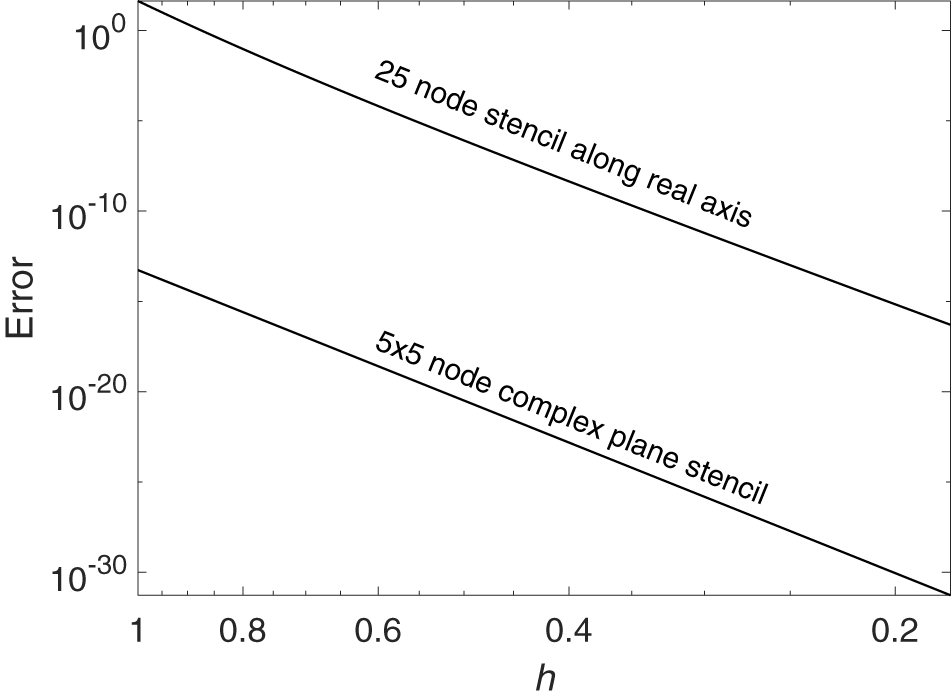
 $O$-symbol contains a hidden proportionality constant. This constant is strikingly low for the complex plane FD formulas. As an example, Figure 2 shows the error when approximating
 $\left.\frac{d^{4}}{dz^{4}}e^{2z}\right|_{z=0}$ with centred 25-node stencils (extending along the real axis vs. in a
 $5\times5$ complex plane square layout). The slopes of the two lines are very similar, but their vertical shift shows a gain of 15 orders of magnitude. Since complex plane FD formulas easily produce results that are accurate to typical machine precision
 $O(10^{-16})$, they are in many cases attractive as alternatives to numerically evaluating exact formulas for derivatives (which for certain functions may be algebraically complicated, if at all available) [Reference Wegert14].
Error comparison between 25-node FD stencils for approximating the  $4^{\textrm{th}}$ derivative, along the real line vs. in the complex plane.

2.3. Magnitude of weights
An explanation for the much better error constant illustrated in Figure 2 can be found in the fact that the weights in complex plane FD formulas decay to zero vastly faster than the  $O(1/k)$ and
 $O(1/k^{2})$ rates mentioned in Section 1.1. For increasing stencil sizes on a unit-spaced grid, the magnitude of the complex plane FD stencil weight at location
 $\mu+i\nu$,
 $\mu,\nu$ integer, is of size
 $O(e^{-\frac{\pi}{2}(\mu^{2}+\nu^{2})})$, proven in different ways in [Reference Fornberg3] and [Reference Fornberg4]. Already about 6 node points away from the stencil centre, weights for complex plane FD stencils fall below typical machine precision.
3. Gregory’s quadrature formulas
3.1. The classical Gregory quadrature formulas
Already 70 years before the EML formula was discovered, Gregory understood that the errors of TR, to all algebraic orders, arise from the interval endpoints. His idea was to look for improved TR formulas (here focusing on the left end of an integration interval and for simplicity of notation using step  $h=1$) of the form
 \begin{equation}
\int_{0}^{\infty}f(x)dx\sim\left(\sum_{k=0}^{\infty}f(k)\right)+\left[b_{0}\varDelta^{0}+b_{1}\varDelta^{1}+b_{2}\varDelta^{2}+\ldots\right]\,f(0)\;
\end{equation}
where  $\varDelta$ represents a forward difference, i.e.,
 \begin{equation}
\begin{array}{ll}
\varDelta^{0}f(0) & =f(0)\\
\varDelta^{1}f(0) & =f(1)-f(0)\\
\varDelta^{2}f(0) & =f(2)-2f(1)+f(0)\\
\varDelta^{3}f(0) & =f(3)-3f(2)+3f(1)-f(0)\\
\quad\vdots & \qquad\vdots
\end{array}
\end{equation}
By the method of generating functions (substitute  $f(x)=e^{-z\:x}$ into (12) followed by the variable change
 $w=(1-e^{-z})$ and series expansion about
 $w=0$), it follows by equating coefficients that
 \begin{equation}
b_{0}=-\frac{1}{2},\;b_{1}=\frac{1}{12},\;b_{2}=-\frac{1}{24},\;b_{3}=\frac{19}{720},\;b_{4}=-\frac{3}{160},\;b_{5}=\frac{863}{60480},\;b_{6}=-\frac{275}{24192},\ldots
\end{equation}
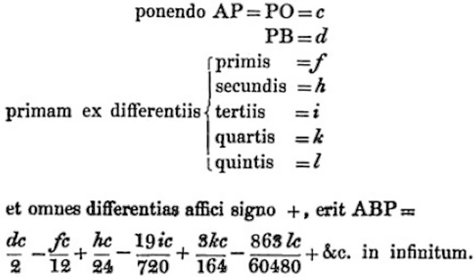
The passage shown in Figure 3 appears in a letter that James Gregory wrote in 1670. We recognize here exactly the same content as in (12), (13) and (14).
Brief extract from the bottom of page 208 and the top of page 209 in [Reference Rigaud11], transcribing a letter from Gregory to Collins dated November 23, 1670. There is a mistake in the next-to-last denominator - should be 160 instead of 164.

Figure 3 Long description
Scanned printed text in an old-style serif typeface. ponendo AP equals PO equals c; PB equals d; { primis equals f, secundis equals h, tertiis equals i, quartis equals k, quintis equals l } prima ex differentiis et omnes differentias affici signo plus, erit ABP equals (dc) divided by 2 minus (fc) divided by 12 plus (hc) divided by 24 minus (19ic) divided by 720 plus (3kc) divided by 164 minus (868lc) divided by 60480 plus etc., in infinitum.
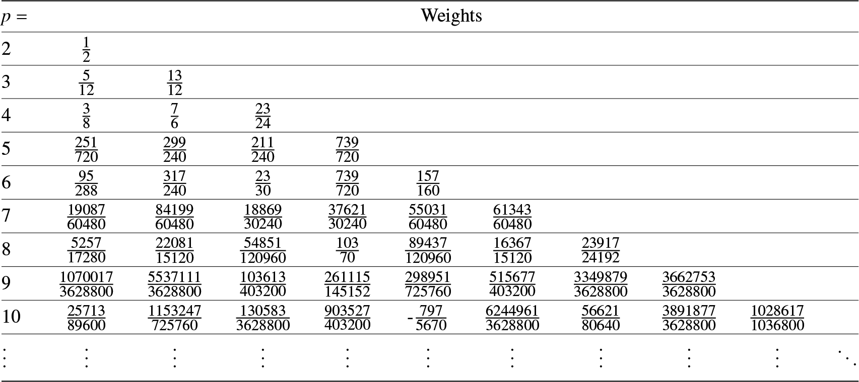
Table 3 gives the nontrivial Gregory weights up through accuracy order  $p=10$ (to be followed by ones, and all multiplied by the step length
 $h$). For order
 $p$, these are obtained by truncating the last sum in (12) after the term
 $b_{p-1}\varDelta^{p-1}$. In case of a finite interval, the weights are used in reversed order at the right end. In the top line, corresponding to accuracy order
 $p=2$, we recognize the TR. Corrections to all weights equal to one from the two ends can overlap.
The non-trivial Gregory weights up through order p  $=10$ (for the left end of an interval, to be followed by ones). The middle entry for accuracy order p
 $=10$ shows the first occurrence of a negative weight

Table 3 Long description
The table lists the non-trivial Gregory endpoint weights for increasing accuracy orders from 2 through 10, with each row giving the sequence of weights used at the left end of an interval. As the order increases, the number of listed weights grows from 1 weight at order 2 to 9 weights at order 10. Most weights are positive fractions and many are close to 1, especially in the later positions of each row. Early rows show simple fractions, while higher orders use larger numerators and denominators, indicating more complex coefficients. A notable exception occurs at order 10, where the fifth listed weight is negative, marking the first negative entry in the table. The final row uses ellipses to indicate that the pattern continues beyond order 10 and that additional weights exist for higher orders.
Numerical analysis textbooks from about half a century or more ago routinely describe Gregory’s method, while modern textbooks typically omit it (in favour of the Newton-Cotes approach, possibly for the unsatisfactory reason that its error analysis is more elementary). Error analysis for Gregory’s quadrature method is given in [Reference Martensen9].
3.2. Gregory quadrature formulas extended to the complex plane
Method 1: The derivatives in (4) can be approximated by complex plane FD stencils. One decides on a stencil size (such as  $3\times3$ or
 $5\times5$) and then approximates as many terms/derivatives as that size permits, followed by adding these up according to their coefficients.
With no loss of generality, we set  $x_{0}=0$ and schematically write the regular TR in the style of (2) as
 \begin{equation}
\int_{0}^{\infty}f(x)dx=h\left\{\frac{1}{2}{\quad{{1}\quad{{1}}\quad{{1}}\quad{{1}}\quad{{1}}},\;\ldots\ldots}\right\} f+O(h^{2}).
\end{equation}
For example, with  $3\times3$ stencils, odd-order derivatives up through
 $f^{(7)}(0)$ can be approximated. Added together, we obtain an end correction to the trapezoidal rule (TR) that can similarly be summarized as
 \begin{equation}\begin{aligned}
\int_{0}^{\infty}f(x)dx=h\left\{\left[{\begin{array}{ccc}
{{\boxed{\tfrac{-821-779i}{403200}}}} & {{{\boxed{{-\tfrac{1889i}{100800}}}}}} & {{\boxed{\tfrac{821-779i}{403200}}}}\\
{{{{\boxed{{-\tfrac{1511}{100800}}}}}}} & {{\left\{\begin{array}{c}
\\
\\
\end{array}\right.\dfrac{1}{2}\begin{array}{c}
\\
\\
\end{array}}} & 1\;{{{\boxed{{+\tfrac{1511}{100800}}}}}}\\
{{{\boxed{{\tfrac{-821+779i}{403200}}}}}} & {{{\boxed{{\tfrac{1889i}{100800}}}}}} & {{{\boxed{{\tfrac{821+779i}{403200}}}}}}
\end{array}}\right]{\quad{{1}\quad{{1}}\quad{{1}}\quad{{1}}},\;\ldots\ldots}\left.\begin{array}{c}\\
\\
\end{array}\right\} \right\} f+O(h^{10}),
\end{aligned}
\end{equation}
where the added correction terms have been boxed. This approach is discussed in [Reference Fornberg2], in the context of integrating an analytic function along finite line segments on an equi-spaced grid. With a  $5\times5$ stencil, the accuracy becomes
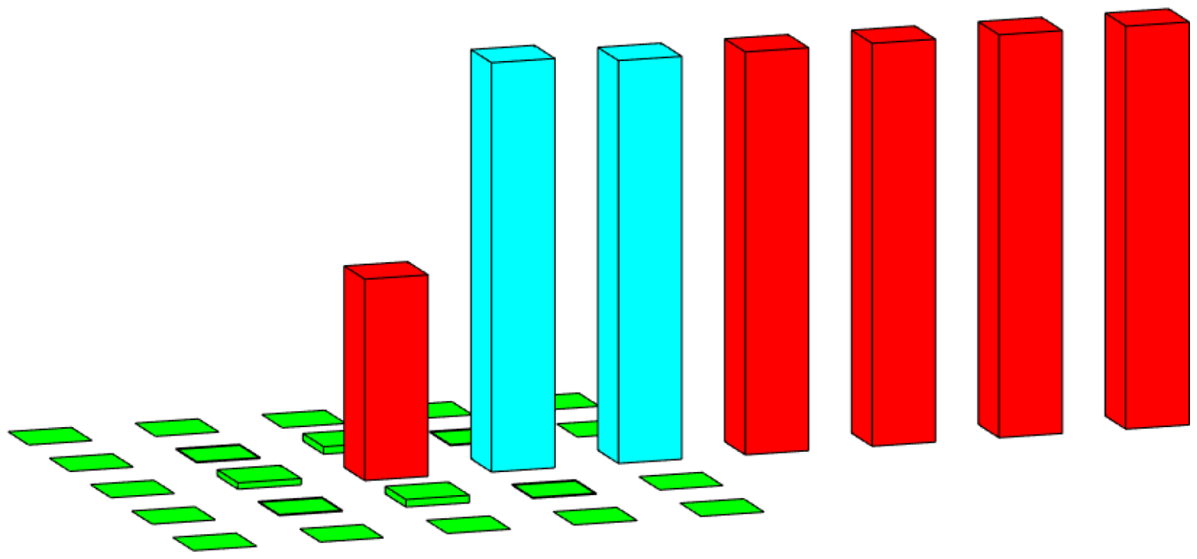
 $O(h^{26})$. Roughly speaking, the grid density needed for a reasonably resolved graphical display of a function turns out to be comparable to what is needed for double precision integration accuracy. Figure 4 illustrates that the correction coefficients are numerically very small compared to the regular weights in the TR.
Illustration of the magnitudes of the weights in the  $5\times5$ case of TR end correction. Entries belonging to the TR formula are shown in red, to the correction stencil in green, and the overlapping entries in blue. Compared to the TR weights (1/2 at the end point(s), and 1 otherwise), the correction stencil weights are two (or more) orders of magnitude smaller. The exact correction weights in this
 $5\times5$ stencil case are given in [Reference Fornberg2].

Method 2: This produces identical TR corrections more directly, as it requires no knowledge of the EML expansion. The LHS of (12), applied to  $e^{z\,\xi}$, becomes (when converging)
 $\int_{0}^{\infty}e^{z\,\xi}dz-h\sum_{k=0}^{\infty}e^{kh\xi}=\frac{h}{e^{h\,\xi}-1}-\frac{1}{\xi}$. With correction stencil nodes at
 $z_{k},$
 $k=1,2,\ldots,N$, match as many powers of
 $\xi$ as possible between the Taylor expansion of this function and of
 $\sum_{k=1}^{N}w_{k}e^{z_{k}\,\xi}$.
4. FD formulas for harmonic functions
Attempts to generalize complex variables to higher dimensions (e.g., quaternions) lead to severe restrictions, such as loss of commutativity for multiplication, absence of a counterpart to Cauchy’s integral formula, etc. However, a key feature of analytic functions is that their real and imaginary parts are harmonic functions (i.e., satisfy Laplace’s equation). Harmonic functions are ubiquitous also in higher-dimensional physical applications (e.g., for the components of gravitational and electric fields). For this class of functions, specialized FD stencils with some similarity to the ones for analytic functions are again available. We describe next a couple of approaches for constructing such formulas before listing some illustrative examples.
4.1. FD stencil generation via Taylor expansions
As a starting point, we can note that all the coefficients in (10) are real (which is not the case for any of the lower-order derivatives). This stencil will thus approximate  $f^{(4)}(0)$ with accuracy
 $O(h^{8})$ for any real-valued 2-D harmonic function, without the need for any knowledge about a matching harmonic conjugate part. Direct Taylor expansion verifies this, since
 \begin{align}
&\color{red}{\frac{3}{10h^{4}}
\left[
\begin{array}{ccc}
-1 & 16 & -1\\
16 & -60 & 16\\
-1 & 16 & -1
\end{array}
\right]f}
\nonumber\\
&\quad=
\frac{21}{5h^{2}}
\color{green}{\left(
\frac{\partial^{2}}{\partial x^{2}}
+\frac{\partial^{2}}{\partial y^{2}}
\right)}f
+\color{red}{\frac{\partial^{4}f}{\partial x^{4}}}
-\frac{1}{20}
\left(
13\frac{\partial^{2}}{\partial x^{2}}
-7\frac{\partial^{2}}{\partial y^{2}}
\right)
\color{green}{\left(
\frac{\partial^{2}}{\partial x^{2}}
+\frac{\partial^{2}}{\partial y^{2}}
\right)}f
\nonumber\\
&\quad+
\frac{3h^{2}}{1800}
\left(
7\frac{\partial^{4}}{\partial x^{4}}
-22\frac{\partial^{4}}{\partial x^{2}\partial y^{2}}
+7\frac{\partial^{4}}{\partial y^{4}}
\right)
\color{green}{\left(
\frac{\partial^{2}}{\partial x^{2}}
+\frac{\partial^{2}}{\partial y^{2}}
\right)}f
\nonumber\\
&\quad+
\frac{3h^{4}}{14400}
\left(
\frac{\partial^{2}}{\partial x^{2}}
-2\frac{\partial^{2}}{\partial x\partial y}
-\frac{\partial^{2}}{\partial y^{2}}
\right)
\left(
\frac{\partial^{2}}{\partial x^{2}}
+2\frac{\partial^{2}}{\partial x\partial y}
-\frac{\partial^{2}}{\partial y^{2}}
\right)
\color{green}{\left(
\frac{\partial^{2}}{\partial x^{2}}
+\frac{\partial^{2}}{\partial y^{2}}
\right)^{2}}f
\nonumber\\
&\quad+
\frac{3h^{6}}{907200}
\left(
7\frac{\partial^{8}}{\partial x^{8}}
-52\frac{\partial^{8}}{\partial x^{6}\partial y^{2}}
-158\frac{\partial^{8}}{\partial x^{4}\partial y^{4}}
-52\frac{\partial^{8}}{\partial x^{2}\partial y^{6}}
+7\frac{\partial^{8}}{\partial y^{8}}
\right)
\color{green}{\left(
\frac{\partial^{2}}{\partial x^{2}}
+\frac{\partial^{2}}{\partial y^{2}}
\right)}f
\nonumber\\
&\qquad+
\color{red}{O(h^{8})}.
\end{align}
On the second line, we see  $\frac{\partial^{4}f}{\partial x^{4}}$, and all other terms up to the final
 $O(h^{8})$ have
 $\left(\frac{\partial^{2}}{\partial x^{2}}+\frac{\partial^{2}}{\partial y^{2}}\right)f$ as factor, i.e., vanish when the stencil is applied to a harmonic function. This second line could alternatively have been written as
 ${\color{red}+}{\color{red}{\frac{\partial^{4}f}{\partial y^{4}}}}+\frac{1}{20}\left(7\frac{\partial^{2}}{\partial x^{2}}-13\frac{\partial^{2}}{\partial y^{2}}\right){\color{green}{\left(\frac{\partial^{2}}{\partial x^{2}}+\frac{\partial^{2}}{\partial y^{2}}\right)}}f$, consistent with the fact that, for
 $f(x,y)$ harmonic,
 $\frac{\partial^{4}f}{\partial x^{4}}=\frac{\partial^{4}f}{\partial y^{4}}$. The expansion suggests a strategy for creating FD stencils that are specific to harmonic functions (and not just for the
 $4^{\textrm{th}}$ derivative as in this example). If a 2-D FD stencil is to be accurate for all 2-D functions
 $f(x,y),$ all error terms up through its accuracy order need to vanish identically. The requirement for harmonic function-specific stencils is much milder - successive error terms need just contain
 $\left(\frac{\partial^{2}}{\partial x^{2}}+\frac{\partial^{2}}{\partial y^{2}}\right)$ as a factor (similarly the factor
 $\left(\frac{\partial^{2}}{\partial x^{2}}+\frac{\partial^{2}}{\partial y^{2}}+\frac{\partial^{2}}{\partial z^{2}}\right)$ in 3-D, etc.). With a symbolic algebra system (such as Mathematica and Maple), it is straightforward to create stencil weights with this type of error expansions. One finds, for example:
 \begin{equation*}
\left[\begin{array}{ccc}
0 & 1 & 0\\
1 & 2 & 1\\
0 & 1 & 0\\
\hline 0 & 0 & 0\\
0 & 0 & 0\\
0 & 0 & 0\\
\hline 0 & -1 & 0\\
-1 & -2 & -1\\
0 & -1 & 0
\end{array}\right]\frac{f}{12h}=\frac{\partial f}{\partial z}+\frac{h^{2}}{6}\frac{\partial}{\partial z}\left(\frac{\partial^{2}}{\partial x^{2}}+\frac{\partial^{2}}{\partial y^{2}}+\frac{\partial^{2}}{\partial z^{2}}\right)f+O(h^{4})
\end{equation*}
and
 \begin{equation*}
\left[\begin{array}{ccc}
0 & 1 & 0\\
1 & 8 & 1\\
0 & 1 & 0\\
\hline 0 & -2 & 0\\
-2 & -16 & -2\\
0 & -2 & 0\\
\hline 0 & 1 & 0\\
1 & 8 & 1\\
0 & 1 & 0
\end{array}\right]\frac{f}{12h^{2}}=\frac{\partial^{2}f}{\partial z^{2}}+\frac{h^{2}}{12}\frac{\partial^{2}}{\partial z^{2}}\left(\frac{\partial^{2}}{\partial x^{2}}+\frac{\partial^{2}}{\partial y^{2}}+\frac{\partial^{2}}{\partial z^{2}}\right)f+O(h^{4}).
\end{equation*}
By rotating these stencils, we immediately obtain similar approximations for derivatives in the other spatial directions. Corresponding  $5\times5\times5$ stencils become accurate to
 $O(h^{10})$. Vast number of variations are available, such as
 $5\times5\times3$ stencils, different grid spacings in the different spatial directions, etc.
4.2. FD stencil generation via basis function expansions
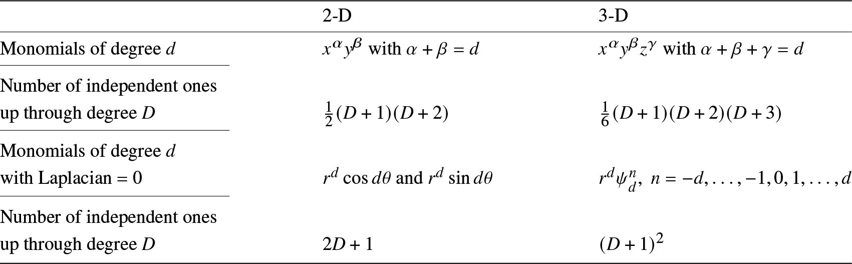
As noted above, a simple approach to calculating FD weights is to form the linear system that enforces the exact result for monomials up to a desired degree. Table 4 compares how many such monomials there are in 2-D and 3-D, in cases when we want to obtain stencils that are accurate for arbitrary functions vs. when we are only interested in harmonic functions. For any number of stencil weights, it is clear from the table how high the degree of monomials will be that can be accommodated exactly. The FD stencils obtained by solving the resulting linear system need not be grid based.
Number of independent monomials without and with the constraint that Laplacian equals to zero

Table 4 Long description
The table compares how many independent polynomial-like terms exist in two dimensions versus three dimensions, both with no constraint and with the constraint that the Laplacian is zero. Without the constraint, it counts all monomials up to a chosen maximum degree, giving a quadratic growth pattern in two dimensions and a cubic growth pattern in three dimensions. With the Laplacian-zero constraint, it instead counts harmonic terms: in two dimensions these come as paired sine and cosine angular modes for each degree, while in three dimensions they come as spherical-harmonic modes spanning orders from negative degree through positive degree. Under this constraint, the number of independent terms up to the maximum degree grows linearly in two dimensions and quadratically in three dimensions. Overall, the constraint greatly reduces the number of independent terms compared with the unconstrained case, and it changes the growth rate in both dimensions. The counts are expressed as functions of the maximum degree, so the table conveys trends rather than specific numeric totals for a particular degree.
4.3. Magnitude of stencil weights
As noted in Section 1.1, the magnitude of standard FD weights decay very slowly with the distance from the stencil centre. The complex case (Section 2.3) is strikingly different, with stencils of increasing order staying highly local. FD stencils specific to harmonic functions fall in-between these two cases. Precise formulas are presently lacking, but numerical calculations suggest exponential decay rates - sufficient to make derivative approximations well localized (further discussed and illustrated in [Reference Fornberg and Jacobs7]).
5. Conclusions
While all the ingredients in the present discussion (finite differences, the trapezoidal rule, the complex plane, analytic and harmonic functions, etc.) have long histories, there has been surprisingly little attention paid in the past to consider certain combinations, such as finite differences applied as 2-D stencils in the complex plane. We have here noted that such combinations can provide very effective novel computational opportunities, still insufficiently explored. One recent application concerns numerical approximation of fractional order derivatives of analytic functions [Reference Fornberg and Piret8].
Appendix: Examples of size
$5\times5$ stencils for analytic functions

 \begin{equation*}
f'(0)=\frac{1}{h}\left[\begin{array}{ccccc}
\frac{1+i}{477360} & \frac{4(-1-i)}{29835} & \frac{i}{1326} & \frac{4(1-i)}{29835} & \frac{-1+i}{477360}\\
\frac{4(-1-i)}{29835} & \frac{8(-1-i)}{351} & \begin{array}{c}
\\
\\
\end{array}\frac{-8i}{39}\begin{array}{c}
\\
\\
\end{array} & \frac{8(1-i)}{351} & \frac{4(1-i)}{29835}\\
\frac{1}{1326} & \frac{-8}{39} & 0 & \frac{8}{39} & \frac{-1}{1326}\\
\frac{4(-1+i)}{29835} & \frac{8(-1+i)}{351} & \begin{array}{c}
\\
\\
\end{array}\frac{8i}{39}\begin{array}{c}
\\
\\
\end{array} & \frac{8(1+i)}{351} & \frac{4(1+i)}{29835}\\
\frac{1-i}{477360} & \frac{4(-1+i)}{29835} & \frac{-i}{1326} & \frac{4(1+i)}{29835} & \frac{-1-i}{477360}
\end{array}\right]f+O(h^{24}),
\end{equation*}
 \begin{equation*}
f''(0)=\frac{1}{h^{2}}\left[\begin{array}{ccccc}
\frac{-i}{477360} & \frac{8(-1+3i)}{149175} & \frac{1}{1326} & \frac{8(-1-3i)}{149175} & \frac{i}{477360}\\
\frac{8(1+3i)}{149175} & \frac{16i}{351} & \begin{array}{c}
\\
\\
\end{array}\frac{-16}{39}\begin{array}{c}
\\
\\
\end{array} & \frac{-16i}{351} & \frac{8(1-3i)}{149175}\\
\frac{-1}{1326} & \frac{16}{39} & 0 & \frac{16}{39} & \frac{-1}{1326}\\
\frac{8(1-3i)}{149175} & \frac{-16i}{351} & \begin{array}{c}
\\
\\
\end{array}\frac{-16}{39}\begin{array}{c}
\\
\\
\end{array} & \frac{16i}{351} & \frac{8(1+3i)}{149175}\\
\frac{i}{477360} & \frac{8(-1-3i)}{149175} & \frac{1}{1326} & \frac{8(-1+3i)}{149175} & \frac{-i}{477360}
\end{array}\right]f+O(h^{24}),
\end{equation*}
 \begin{equation*}
f^{(3)}(0)=\frac{1}{h^{3}}\left[\begin{array}{ccccc}
\frac{-1+i}{636480} & \frac{8(7-i)}{248625} & \frac{-i}{884} & \frac{8(-7-i)}{248625} & \frac{1+i}{636480}\\
\frac{8(1-7i)}{248625} & \frac{8(1-i)}{117} & \begin{array}{c}
\\
\\
\end{array}\frac{16i}{13}\begin{array}{c}
\\
\\
\end{array} & \frac{8(-1-i)}{117} & \frac{8(-1-7i)}{248625}\\
\frac{1}{884} & \frac{-16}{13} & 0 & \frac{16}{13} & \frac{-1}{884}\\
\frac{8(1+7i)}{248625} & \frac{8(1+i)}{117} & \begin{array}{c}
\\
\\
\end{array}\frac{-16i}{13}\begin{array}{c}
\\
\\
\end{array} & \frac{8(-1+i)}{117} & \frac{8(-1+7i)}{248625}\\
\frac{-1-i}{636480} & \frac{8(7+i)}{248625} & \frac{i}{884} & \frac{8(-7+i)}{248625} & \frac{1-i}{636480}
\end{array}\right]f+O(h^{24}),
\end{equation*}
 \begin{equation*}
f^{(4)}(0)=\frac{1}{h^{4}}\left[\begin{array}{ccccc}
\frac{1}{318240} & \frac{32(-9-13i)}{1243125} & \frac{-1}{442} & \frac{32(-9+13i)}{1243125} & \frac{1}{318240}\\
\frac{32(-9+13i)}{1243125} & \frac{-32}{117} & \begin{array}{c}
\\
\\
\end{array}\frac{64}{13}\begin{array}{c}
\\
\\
\end{array} & \frac{-32}{117} & \frac{32(-9-13i)}{1243125}\\
\frac{-1}{442} & \frac{64}{13} & \frac{-92937}{5000} & \frac{64}{13} & \frac{-1}{442}\\
\frac{32(-9-13i)}{1243125} & \frac{-32}{117} & \begin{array}{c}
\\
\\
\end{array}\frac{64}{13}\begin{array}{c}
\\
\\
\end{array} & \frac{-32}{117} & \frac{32(-9+13i)}{1243125}\\
\frac{1}{318240} & \frac{32(-9+13i)}{1243125} & \frac{-1}{442} & \frac{32(-9-13i)}{1243125} & \frac{1}{318240}
\end{array}\right]f+O(h^{24}).
\end{equation*}
For this stencil size, one can approximate up through  $f^{(24)}(0)$, which becomes fourth order accurate.









 Open access

