1 Introduction
Electron heating mechanisms in capacitive discharges are widely discussed in the literature (Lieberman & Lichtenberg Reference Lieberman and Lichtenberg2005; Chabert & Braithwaite Reference Chabert and Braithwaite2011). In the commonly accepted models at low pressure, the stochastic heating resulting from the interaction of the electrons with the oscillating sheath dominates. During the expansion of the sheaths the electrons close to the electrodes are accelerated, forming beams that transfer energy to the plasma bulk. The beams are observed both experimentally and in particle-in-cell (PIC) models (see e.g. Vender & Boswell Reference Vender and Boswell1990; Schulze et al. Reference Schulze, Schüngel, Donkó, Luggenhölscher and Czarnetzki2010). Generation of multiple beams during one phase of the sheath expansion is studied in (Vender & Boswell Reference Vender and Boswell1992; Wilczek et al. Reference Wilczek, Trieschmann, Schulze, Schuengel, Brinkmann, Derzsi, Korolov, Donkó and Mussenbrock2015, Reference Wilczek, Trieschmann, Eremin, Brinkmann, Schulze, Schuengel, Derzsi, Korolov, Hartmann and Donkó2016). The ohmic heating is the governing mechanism at higher pressures.
Despite the fact that the heating mechanisms have been studied for decades, recently, a series of new results contributed significantly to their better understanding, changing even the basis of the traditional models. From the first two moments of the Boltzmann equation the importance of the role of the pressure heating is outlined (Turner Reference Turner1995; Lafleur, Chabert & Booth Reference Lafleur, Chabert and Booth2014; Lafleur & Chaber Reference Lafleur and Chaber2015). Applying the same method, in Schulze et al. (Reference Schulze, Donkó, Lafleur, Wilczek and Brinkmann2018), it is shown that the ambipolar electric fields outside the sheaths play a key role in the electron power absorption.
Depending on the role of the secondary electrons, alpha and gamma modes are distinguished. In the alpha mode at relatively low applied voltage the ionization is in the plasma volume. At higher voltage a transition to the gamma mode, in which the secondary electrons play an important role, is observed. Additionally, the case when the ionization is caused mainly by ohmic heating is called the omega mode (Hemke et al. Reference Hemke, Eremin, Mussenbrock, Derzsi, Donkó, Dittmann, Meichsner and Schulze2013). Specific modes observed in discharges in electronegative gases are the drift-ambipolar operation mode in Schulze et al. (Reference Schulze, Derzsi, Dittmann, Hemke, Meichsner and Donkó2011) and striation mode in Liu et al. (Reference Liu, Schüngel, Korolov, Donkó, Wang and Schulze2016, Reference Liu, Korolov, Schüngel, Wang, Donkó and Schulze2017). The mode transition leads to changes of the plasma density and average electron energy, the profile of the electron concentration and of the electron energy probability function (EEPF).
The mode transitions are studied both experimentally and theoretically. In the experiments, probe diagnostics are widely used (Godyak, Piejak & Alexandrovich Reference Godyak, Piejak and Alexandrovich1992) for the determination of the EEPF and optical emission spectroscopy, and especially phase resolved optical emission spectroscopy (PROES), for the dynamics of the excitation processes (Schulze et al. Reference Schulze, Schüngel, Donkó, Luggenhölscher and Czarnetzki2010).
The results in Schulze et al. (Reference Schulze, Derzsi, Dittmann, Hemke, Meichsner and Donkó2011) show that, in addition to the electron beams in the expanding sheaths in argon discharges, in electronegative discharges ionization inside the plasma bulk is also observed. The result is explained by the strong drift electric field in the discharge centre due to the low direct current (dc) conductivity caused by the low electron concentration. In the current work, a strong drift electric field in the discharge centre is obtained in argon discharge. In contrast to the electronegative discharges in Schulze et al. (Reference Schulze, Derzsi, Dittmann, Hemke, Meichsner and Donkó2011) the low electron concentration here is due to the radial particle losses in a small radius discharge tube. The simultaneously acting ohmic and stochastic heating are discussed also in Kawamura, Lieberman & Lichtenberg (Reference Kawamura, Lieberman and Lichtenberg2014). In our paper it is demonstrated that each of the two mechanisms could dominate in different parts of the discharge, causing the corresponding changes of the plasma parameters.
The motivation for the current work is the experimental results in Tarnev et al. (Reference Tarnev, Koleva, Lishev, Paunska, Iordanova and Shivarova2012). A small-radius planar-coil inductively driven discharge in hydrogen for fusion application (Lishev et al.
Reference Lishev, Paunska, Shivarova and Tarnev2012) is studied by PROES. As is known, the capacitive mode of the inductive discharge is similar to a capacitive discharge. The experimental results show that the time variation of the
 $H_{\unicode[STIX]{x1D6FC}}$
spectral line intensity could be approximated by a sum of two functions
 $f=f_{1}+f_{2}$
. The first function
 $f_{1}=A_{1}\sin \unicode[STIX]{x1D714}t$
for
 $\sin \unicode[STIX]{x1D714}t>0$
and 0 for
 $\sin \unicode[STIX]{x1D714}t<0$
resembles the light intensity caused by the electron beams, i.e. one maximum per radio-frequency (rf) period close to each electrode. The second function is
 $f_{2}=A_{2}\sin ^{2}(\unicode[STIX]{x1D714}t+\unicode[STIX]{x1D719}_{0})$
with two maxima per rf period which describes the modulation of the energy in the case of sinusoidal variation of the electric field. The first interpretation of the experimental results was that this is an E- to H- mode transition in an inductive discharge but later it was found that it is a result of a superposition of two different heating mechanisms in a capacitive mode. Part of the experimental results not published in Tarnev et al. (Reference Tarnev, Koleva, Lishev, Paunska, Iordanova and Shivarova2012) are presented in § 4.
The goal of the model developed in the current work is to prove that in small radius capacitive discharges with a large distance between the electrodes the two heating mechanisms – stochastic heating in the sheath-plasma boundary and ohmic heating in the plasma bulk – could act simultaneously. The distance between the electrodes is increased to 15 cm in contrast to the traditionally studied cases with a discharge gap of a few centimetres. A wide range of tube radii from infinity to 1.5 cm is studied at low pressures of 2.5–40 Pa.
Strictly speaking, the modelling of small radius capacitive discharges requires a three-dimensional (3-D) or at least 2-D axisymmetric model. Here, a simpler approach is used. The model is one-dimensional and works with radially averaged values of the plasma parameters. The radial particle losses are estimated assuming ambipolar diffusion in the radial direction.
The paper is structured as follows. In § 3.1 the case of infinite radius is studied for the role of the pressure and the distance between the electrodes. In 3.2 the distance between the electrodes is 15 cm and the tube radius is reduced to very small values. In 3.3 the dependence on the pressure for the case of small radius and large gap is investigated. In § 4 are presented experimental results.
2 Description of the model
The developed model is a 1D3v (one dimensional in space and three dimensional in velocity space) particle-in-cell model with Monte Carlo collisions (PIC/MCC) (Verboncoeur Reference Verboncoeur2005; Longo Reference Longo2006; Turner Reference Turner2006; Donkó Reference Donkó2011). A radio frequency voltage
 $U=U_{0}\cos \unicode[STIX]{x1D714}t$
with amplitude
 $U_{0}=150~\text{V}$
and frequency 13.56 MHz are applied at the left electrode. The right electrode is grounded. The distance
 $L$
between the electrodes is divided into 1000 cells for
 $L=3~\text{cm}$
and 4500 cells for
 $L=15~\text{cm}$
. For the plasma densities in the model, the Debye length is several times bigger than the cell size. As the goal of the model is to describe the basic properties of long capacitive discharges, the model is in argon with a relatively small number of elementary processes taken into account. Elastic collisions with neutral atoms and inelastic collisions for excitation and ionization are considered for the electrons and elastic and charge exchange collisions for the ions. The data for the cross-sections are from Phelps (Reference Phelps1994, Reference Phelps2017). The null-collision method is applied. The particles that reach one of the electrodes are removed from the simulation. Secondary electrons and electron–electron collisions are not included in the model.
In § 3.1 the case of infinite radius is studied, i.e. the radial losses are neglected and the discharge is described by a 1-D model, as is usual in PIC models of capacitive discharges. In the case of small discharge radius in §§ 3.2 and 3.3 the radial particle losses are estimated using the following procedure. First, the average electron energy
 $\langle E_{k}\rangle$
is calculated and then the effective electron temperature
 $T_{e\,eff}$
is determined from
 $\langle E_{k}\rangle =3/2kT_{e\,eff}$
(
 $k$
is the Boltzmann constant) and the ambipolar diffusion coefficient
 $D_{A}$
is calculated with this temperature. Assuming a Bessel radial profile of the plasma density
 $$\begin{eqnarray}n=n_{0}\text{J}_{0}\left(\frac{2.4}{R}r\right)\end{eqnarray}$$
the number of the electron and ion superparticles
 $N_{wall}$
lost on the side wall in a time step
 $\unicode[STIX]{x0394}t$
is given by:
 $$\begin{eqnarray}N_{wall}=ND_{A}\left(\frac{2.4}{R}\right)^{2}\unicode[STIX]{x0394}t.\end{eqnarray}$$
 $N$
is the total number of the ion superparticles,
 $R$
is the discharge radius and 2.4 is the first zero of the Bessel function
 $\text{J}_{0}$
. The superparticles removed from the simulation are randomly chosen. A more precise approach requires the electrons with the highest radial energy (i.e. with the highest total energy calculated from the sum of the kinetic energy of the radial velocity components and of the potential energy in the radial ambipolar potential) to be removed from the simulation. Working with radially averaged values of the plasma parameters the energy of the electrons in the radial ambipolar potential is not known and the total energy could not be calculated in our model. Therefore, our model estimates correctly the particle flux to the side wall and underestimates the electron energy flux.
The simulation starts with a relatively small number of superparticles with Maxwellian velocity distribution with temperature 2 eV for the electrons and 300 K for the ions. After reaching a quasi-stationary solution, the charge and the mass of each superparticle is divided by 2. The next run of the code starts with an approximately doubled number of superparticles with the velocity and spatial distributions obtained in the previous run. The procedure is repeated until the plasma parameters do not change anymore with the number of superparticles.
After the final solution is reached, the code is run for 10 more rf periods. The results presented in the next section are from these runs averaged over the rf period.
3 Results
3.1 Infinite radius
First, the case of infinite discharge radius is studied, i.e. the radial losses are neglected.
The changes of the profile of the electron concentration with the distance between the electrodes are shown in figure 1. In the case of a relatively small discharge gap of 3 cm and gas pressures of 10 Pa (figure 1
a) and 40 Pa (figure 1
b) a result that is well known from the literature is obtained (see e.g. Hwang, Lee & Lee Reference Hwang, Lee and Lee2014; Sun, Becker & Loffhagen Reference Sun, Becker and Loffhagen2016): with the pressure increase the profile of the electron concentration in the plasma bulk becomes flatter. The increase of the discharge gap leads to a similar result (figure 1
c,d), i.e. the plasma density profile becomes flatter with the gap increase. Therefore, this is an indication that the increased distance between the electrodes acts similarly to the pressure increase. This result is in accordance with the scaling laws, i.e. the gas discharge behaviour depends on the product
 $pL$
.
Profiles of the electron concentration for
 $p=10~\text{Pa}$
and gap 3 cm (a), 10 cm (c), 15 cm (d) and
 $p=40~\text{Pa}$
and gap 3 cm (b).

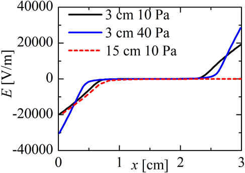
The wall sheaths are clearly seen in the profiles of the electric field in figure 2 which are averaged over the rf period. Comparing the discharges with a gap of 3 cm and pressures 10 Pa and 40 Pa, at the higher pressure the wall sheath is narrower because of the lower mobility of the electrons. As the voltage applied on the left electrode is the same in all cases, the same potential drop on a narrower sheath leads to stronger electric field at 40 Pa. The increase of the discharge gap leads to an increase of the part of the profile with
 $E\approx 0$
(only the first 3 cm of the profile with
 $L=15~\text{cm}$
is shown in figure 2). The small deviations of the profiles of the electric field in the sheath at 10 Pa result from the slightly different plasma density.
Time averaged profile of the electric field. The discharge gaps and the pressures as indicated in the figure.

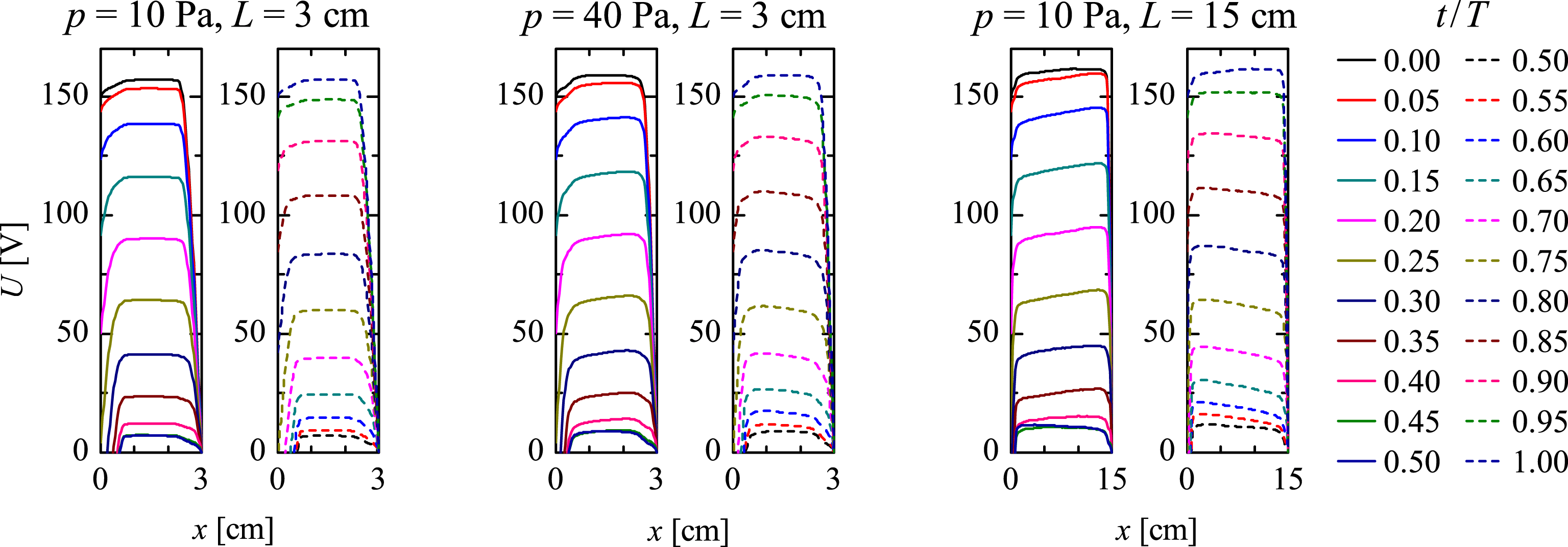
Additional information for the processes in the plasma is provided by the dynamics of the plasma potential in figure 3. As mentioned above, the voltage on the left electrode changes as
 $U=U_{0}\cos \unicode[STIX]{x1D714}t$
with
 $U_{0}=150~\text{V}$
and
 $\unicode[STIX]{x1D714}=2\unicode[STIX]{x03C0}/T$
being the angular frequency. The time interval between the lines of the electric potential in figure 3 is
 $T/20$
. The left figure of each pair represents the first half-cycle (from
 $t=0$
to
 $t=T/2$
, solid lines) when the voltage decreases, while in the right figures the voltage increases (dashed lines). In order to show more clearly the behaviour in the plasma bulk, the presentation is limited only to the positive values of the potential.
Profiles of the potential for pressures and discharge gaps as given in the figure. The interval between the profiles in the figures is
 $T/20$
. The left figure of each pair (solid lines) corresponds to the first half-period when the voltage on the left electrode decreases from
 $+150~\text{V}$
to
 $-150~\text{V}$
. The right figures (dashed lines) are for the second half-cycle when the voltage increases.

In the case
 $p=10~\text{Pa}$
,
 $L=3~\text{cm}$
the potential in the plasma bulk is almost constant, i.e. the electric field
 $E\approx 0$
. For the other two cases in figure 3 there is a gradient of the potential in the bulk and, therefore, non-zero electric field.
According to the general properties of the capacitive discharges the electron velocity in the plasma bulk chances its direction with the changes of the polarity of the voltage on the powered electrode to compensate the external electric field. However, the flow of the electrons is caused by different mechanisms in the three cases in figure 3. At low pressure and small discharge gap the mean free path of the charged particles is large and the electrons accelerated in the expanding sheaths cross the entire plasma bulk, i.e. they move in the central part of the discharge with a certain velocity even at zero local electric field. The plasma conductivity in this case is non-local: the current at a given position depends on the electric field not only at this position but on the field along the entire trajectories of the electrons between two collisions. At higher pressure the mean free path decreases and the electrons from the sheaths cannot penetrate deep into the plasma bulk. The drift velocity there is a result of the local electric field. At low pressure and large discharge gap the mean free path of the charged particles is large but still smaller than the discharge length and the electrons from the sheaths do not reach the discharge centre. In this case the motion of the electrons in the discharge centre also is due to the local electric field.
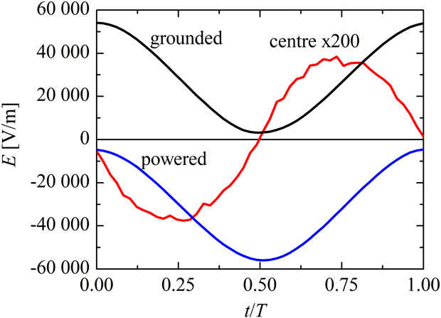
The electric field on the grounded and on the powered electrodes and in the centre of the discharge at
 $x=1.5~\text{cm}$
for
 $p=40~\text{Pa}$
and
 $L=3~\text{cm}$
. In order to be shown on the same graph, the values in the centre are multiplied by a factor of 200.

The electric field in the plasma bulk is shifted in phase with respect to the field close to the electrodes (figure 4). In general, the phase shift depends on the gas discharge conditions as the resistance and the inductance of the plasma bulk depend on the plasma parameters.
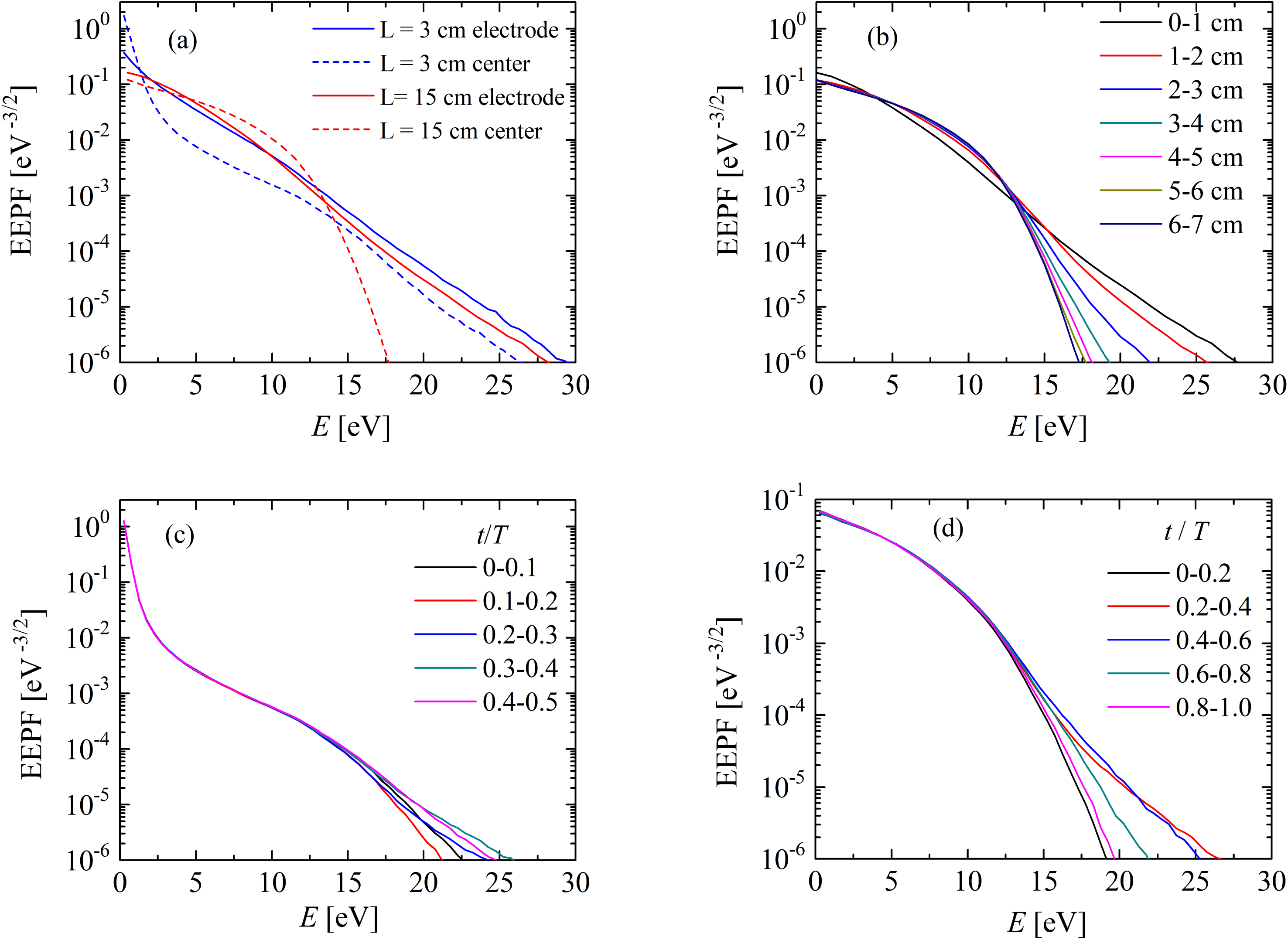
The electric field in the plasma bulk also modifies the EEPF (figure 5). In figure 5(a,b), the EEPF is calculated in small
 $x$
-intervals: 0.5 cm for the case with
 $L=3~\text{cm}$
and 1 cm for the case with
 $L=15~\text{cm}$
. Close to the electrodes the EEPFs are almost straight lines in both cases. However, in the plasma bulk the behaviour is completely different. At small discharge gap the well-known result from the literature (see e.g. Godyak et al.
Reference Godyak, Piejak and Alexandrovich1992; Hwang et al.
Reference Hwang, Lee and Lee2014) for a bi-Maxwellian EEPF is obtained. The two slopes of the EEPF correspond to the high-energy electrons accelerated in the expanding sheaths and to the low-energy electrons trapped between the sheaths. At large discharge gap the result is a Druyvesteyn-like EEPF. In this case, the centre of the discharge is far enough from the electrodes and the electrons accelerated in the sheaths cannot reach it. The EEPF is formed mainly from the local electric field. Here, it should be mentioned that a Druyvesteyn-like EEPF is typical for the positive column of a dc discharge and some rf and microwave discharges at similar conditions in argon (Karoulina & Lebedev Reference Karoulina and Lebedev1988; Kortshagen, Parker & Lawler Reference Kortshagen, Parker and Lawler1996; Petrova et al.
Reference Petrova, Benova, Petrov and Zhelyazkov1999). The transition from Maxwellian to Druyvesteyn-like EEPF is gradual from the electrode to the discharge centre (figure 5
b). The number of high-energy electrons decreases with the distance from the electrodes. In the case
 $p=40~\text{Pa}$
,
 $L=3~\text{cm}$
the electron beams from the sheaths do not reach the central part of the discharge too and the EEPF there is Druyvesteyn-like, determined by the local electric field. The transition from bi-Maxwellian to Druyvesteyn-like EEPF with the pressure is well known from the literature (see e.g. Godyak et al.
Reference Godyak, Piejak and Alexandrovich1992; Hwang et al.
Reference Hwang, Lee and Lee2014). The new effect here is the similar behaviour with the increase of the discharge gap at fixed low pressure. More results for the axial variation of the EEPF are given in Pavlova, Gilev & Tarnev (Reference Pavlova, Gilev and Tarnev2018). The axial variation of the EEPF in capacitive discharges is experimentally observed by Zhu et al. (Reference Zhu, Chen, Li, Cheng and Pu2012).
(a) The EEPF close to the electrodes (solid lines) and in the centre of the discharge (dashed lines) for discharge gaps 3 cm (blue lines) and 15 cm (red lines) and
 $p=10~\text{Pa}$
. (b) Axial variation of the EEPF from the powered electrode to the discharge centre for
 $L=15~\text{cm}$
and
 $p=10~\text{Pa}$
. (c) Time variation of the EEPF for
 $L=3~\text{cm}$
and
 $p=10~\text{Pa}$
in the central part of the discharge between
 $x=1~\text{cm}$
and
 $x=2~\text{cm}$
. (d) Time variation of the EEPF for
 $L=15~\text{cm}$
and
 $p=10~\text{Pa}$
close to the electrode between
 $x=0$
and
 $x=3~\text{cm}$
.

Concentration of the high-energy electrons in
 $\text{m}^{-3}$
(only electrons with energies higher than the ionization energy for argon 15.76 eV are shown). Spatio-temporal plot for
 $p=10~\text{Pa}$
,
 $L=3~\text{cm}$
in (a);
 $p=40~\text{Pa}$
,
 $L=3~\text{cm}$
in (b) and
 $p=10~\text{Pa}$
,
 $L=15~\text{cm}$
in (c). Averaged over the rf period normalized concentration of the high-energy electrons in (d). Case
 $p=10~\text{Pa}$
,
 $L=3$
in black,
 $p=40~\text{Pa}$
,
 $L=3~\text{cm}$
in blue and
 $p=10~\text{Pa}$
,
 $L=15~\text{cm}$
in red.

The electric field in the plasma bulk is important for the transport processes but the high-energy electrons are formed mainly in the expanding sheaths. The concentration of electrons with energies higher than the ionization threshold is shown in figure 6. Spatio-temporal plots in Pavlova et al. (Reference Pavlova, Gilev and Tarnev2018) show a similar distribution for the ionizing collisions. Clearly seen are the electron beams starting from the electrodes in all cases. However, in the case
 $p=10~\text{Pa}$
,
 $L=3~\text{cm}$
in (figure 6
a) the beams cover the entire plasma bulk, while in the other cases they do not reach the plasma centre. At higher pressure, the reason is the decreased electron mobility (figure 6
b). At larger discharge gap (figure 6
c), the beams are even longer than in figure 6(a) but, similarly to the case with higher pressure, the ionization is mainly close to the electrodes (figure 6
d).
The variation of the EEPF during the rf period is shown in figure 5(c,d). In the central part of the discharge (figure 5
c for
 $L=3~\text{cm}$
) the time variation of the EEPF is relatively weak. As the capacitive discharge in our model is symmetric, the effects of the beams from the powered and from the grounded electrode on the EEPF in the central part of the discharge are equivalent and the EEPF there changes with a period of
 $T/2$
. Hence, in figure 5(c) only the first half-period of the rf field is shown. The increase of the high-energy part of the EEPF at
 $t/T=0.3{-}0.4$
(and 0.8–0.9) corresponds to the two beams in figure 6(a). Between the beams at
 $t/T=0.1{-}0.2$
(and 0.6–0.7) the concentration of the high-energy electrons decreases. At larger distances between the electrodes, the role of the beams in the central part of the discharge decreases and the EEPF is almost constant in time. Close to the electrodes the time variation of the EEPF is stronger (figure 5
d for
 $L=15~\text{cm}$
). The high-energy part of the EEPF increases at
 $t/T=0.2{-}0.6$
with the beam from the powered electrode and has a minimum after the beam at
 $t/T=0{-}0.2$
and 0.8–1.0. The behaviour of the EEPF is similar for the other distances between the electrodes.
3.2 The role of the finite radius
In this section the radial particle losses are taken into account. The presented results are for pressure
 $p=10~\text{Pa}$
.
First, a simple analysis based on the continuity equation is performed. Assuming a constant electron temperature in the plasma bulk and constant diffusion coefficient
 $D$
and ionization frequency
 $\unicode[STIX]{x1D708}_{i}$
, the continuity equation in cylindrical coordinates
 $-D\unicode[STIX]{x0394}n_{e}=\unicode[STIX]{x1D708}_{i}n_{e}$
is written in the form
 $$\begin{eqnarray}D\frac{\unicode[STIX]{x2202}^{2}n_{e}}{\unicode[STIX]{x2202}^{2}x}=-\unicode[STIX]{x1D708}_{i}n_{e}-D\unicode[STIX]{x1D6E5}_{r}n_{e}.\end{eqnarray}$$
Here,
 $\unicode[STIX]{x1D6E5}_{r}$
is the radial part of the Laplacian. For a radial Bessel profile of the plasma density of the type
 $n_{e}(x,r)=n_{e0}(x)\text{J}_{0}(2.4r/R)$
 $$\begin{eqnarray}D\frac{\unicode[STIX]{x2202}^{2}n_{e0}(x)}{\unicode[STIX]{x2202}^{2}x}=-\unicode[STIX]{x1D708}_{i}n_{e0}(x)+D\left(\frac{2.4}{R}\right)^{2}n_{e0}(x).\end{eqnarray}$$
Therefore, the sign of the second derivative of
 $n_{e0}$
on the left-hand side of (3.2) is negative when the ionization dominates (first term on the right-hand side) and positive if the radial losses dominate (second term on the right-hand side).
In the case of infinite radius the second term on the right-hand side of (3.2) is zero and the second derivative of
 $n_{e0}$
is negative along the entire discharge (figure 7). As commented above, the maximum of the ionization is close to the electrodes. The number of charged particles created in the plasma bulk is relatively small. However, without volume and radial losses, these particles are lost on the electrodes.
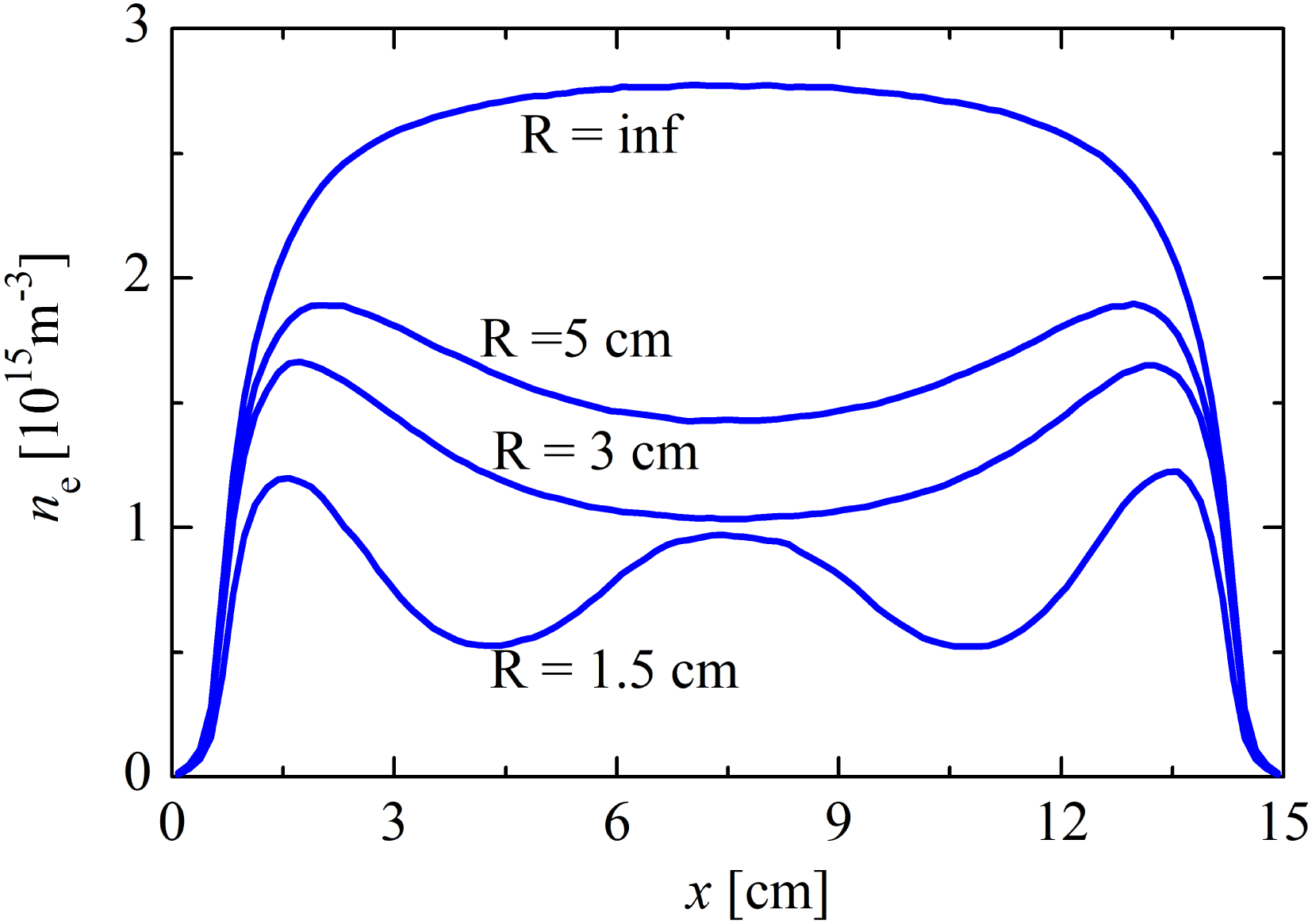
In the case of finite radius, the increased particle losses (due to the radial ambipolar diffusion in the model) lead to lower electron concentration (figure 7). For radii
 $R=5~\text{cm}$
and
 $R=3~\text{cm}$
in the vicinity of the plasma–sheath boundary the ionization is the dominant process in (3.2) and the second derivative of
 $n_{e0}$
is negative. In the main part of the plasma bulk the radial losses dominate and the second derivative of
 $n_{e0}$
is positive. This means that the newly created charged particles in the plasma bulk cannot compensate for the radial losses and a minimum of the electron concentration appears in the discharge centre. The discharge there is sustained mainly by the longitudinal fluxes from the plasma–sheath boundary.
Profiles of the electron concentration averaged over the rf period for
 $p=10~\text{Pa}$
and different discharge radii as indicated in the figure.

The solution of (3.2) in the case
 $\unicode[STIX]{x1D708}_{i}=0$
is of the type
 $$\begin{eqnarray}n_{e0}(x)\sim \exp \left(-\frac{2.4}{R}x\right)\end{eqnarray}$$
i.e. the slopes of the profiles of the decreasing electron concentration from the plasma–sheath boundary to the discharge centre increase with the radius decrease as also figure 7 shows.
A new behaviour is observed at a very small radius (
 $R=1.5~\text{cm}$
in figure 7). A simple analytical model (Heil, Brinkmann & Czarnetzki Reference Heil, Brinkmann and Czarnetzki2008) explains the dependence of the electric field in the plasma bulk on the electron concentration
 $n_{e}$
and electron neutral collision frequency
 $\unicode[STIX]{x1D708}_{m}$
. From the electron momentum equation:
 $$\begin{eqnarray}m_{e}\frac{\text{d}v}{\text{d}t}=eE(t)-m_{e}\unicode[STIX]{x1D708}_{m}v\end{eqnarray}$$
replacing the velocity from the expression for the current density
 $j=en_{e}v$
 $$\begin{eqnarray}E(t)=\frac{m_{e}}{\text{e}^{2}n_{e}}\left(\frac{\text{d}j}{\text{d}t}+v_{m}j\right).\end{eqnarray}$$
Because of the lower electron concentration
 $n_{e}$
, the rf electric field in the discharge centre increases. At
 $R=1.5~\text{cm}$
the field is strong enough to cause significant ionization, which is higher than the radial losses. The sign of the second derivative of the electron concentration in (3.2) is negative and a local maximum at the discharge centre appears.
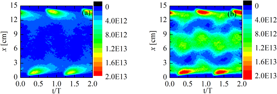
In figure 8 the concentration of the high-energy electrons (with
 $E_{k}>15.76~\text{eV}$
) is shown. For the case
 $R=5~\text{cm}$
(figure 8
a) the electron beams from the sheaths are similar to that in figure 6(c) and only weak variations in the plasma bulk are observed. Completely different is the situation at
 $R=1.5~\text{cm}$
in figure 8(b). In addition to the beams close to the electrodes, there is a maximum of the concentration of the high-energy electrons in the central part of the discharge. The maximum is not stationary and its position and magnitude oscillate with the frequency of the rf field.
Concentration of the high-energy electrons in
 $\text{m}^{-3}$
. Spatio-temporal plot for
 $p=10~\text{Pa}$
,
 $L=15~\text{cm}$
,
 $R=5~\text{cm}$
in (a) and
 $R=1.5~\text{cm}$
in (b).

The finite radius causes changes in the time averaged electric field in the plasma bulk (figure 9). The comparison with the results in figure 7 shows that the field in figure 9 is zero at the positions of the extrema of the electron concentration. According to the general properties of the gas discharges, the direction of the time averaged electric field coincides with the direction of the time averaged particle fluxes. Results in Tarnev & Pavlova (Reference Tarnev and Pavlova2018) also confirm that the shape of the ion velocity profiles coincides with the shape of the time averaged electric field.
Electric field in the plasma bulk averaged over the rf period. The maximum and the minimum values in the sheaths (not shown in the chosen scale in the figure) are at approximately
 $\pm 20\,000~\text{V}~\text{m}^{-1}$
.

In the case of an infinite radius the longitudinal particle flux is directed from the discharge centre to the electrodes. For
 $R=5~\text{cm}$
the longitudinal particle fluxes in the plasma bulk are directed from the maxima at the plasma–sheath boundary to the discharge centre. For
 $R=1.5~\text{cm}$
the charged particles move to the concentration minima at approximately
 $x=4.5~\text{cm}$
and 10.5 cm. Of course, in all cases the particle fluxes in the sheaths are directed to the electrodes.
3.3 The role of the pressure
In this section we present the results for a discharge radius 2 cm and pressure varying from 2.5 Pa to 40 Pa. With the pressure increase the electron concentration increases (figure 10 a) because of the lower diffusion and mobility coefficients and, therefore, reduced particle losses. The two types of electron concentration profiles discussed in the previous section are observed here too. At lower pressures and low electron–neutral collision frequency, according to (3.5), the electric field in the plasma bulk is small. The radial particle losses are high and the ionization does not compensate them. A minimum is formed in the discharge centre. At higher pressure the collision frequency increases, leading to increase of the electric field in the plasma bulk. The increased ionization in the plasma bulk and lower radial losses cause the local maximum in the discharge centre.
With the pressure increase the electron mobility decreases and the electron beams accelerated in the expanding sheaths do not penetrate so deep into the plasma. This is clearly seen from the results in figure 10(a) for the maxima of the electron concentration and in figure 10(b–d) for the concentration of the high-energy electrons. The velocity of the beams also decreases with the pressure.
The results in figure 10(b–d) could be compared with the experimental results in figure 11. As the experimental and modelling results are obtained at very different conditions their comparison is only qualitative, i.e. the structures corresponding to the stochastic and ohmic heating are observed in both cases with similar behaviour. In the experiment the part of the discharge close to the right electrode is not seen by the camera. The results for the concentration of the high-energy electrons in figure 10(b) averaged over the rf period correspond to the results in figure 11(a,b). At the lower pressure of 2.5 Pa the maximum close to the electrode followed by a decrease of the concentration to the plasma bulk is confirmed also by the experimental results in figure 11(a). (The maximum in the experiment is shifted by approximately 1 cm to the right.) At the higher pressure of 20 Pa (figure 11 b) the maximum moves closer to the electrode, as in the model. The second smaller maximum in the plasma bulk is also experimentally observed.
In the analysis of the spatio-temporal plots we should have in mind that the electronics of the camera cause an additional phase shift. At low pressure electron beams accelerated once in a rf period from each electrode are observed in the model (figure 10
c) and in the experiment (figure 11
c). At higher pressure the beams still exists but in addition there is a second heating mechanism in the central part of the discharge. As the variation of the electric field in the discharge is of the type
 $E\sim \cos \unicode[STIX]{x1D714}t$
the energy of the electrons should be modulated as
 $E_{k}\sim \cos ^{2}\unicode[STIX]{x1D714}t$
and two maxima per period should be seen in the spatio-temporal plots. Therefore, the maxima in the central part of the discharge in figures 10(d) and 11(d) result from the electric field in the plasma bulk. In conclusion, the results in figures 10(d) and 11(d) are clear evidence for the simultaneous existence of two heating mechanisms: stochastic heating close to the electrodes and ohmic heating in the plasma bulk.
Profiles of the time averaged electron concentration (a) and concentration of the high-energy electrons (b) at pressures as indicated in the figures. Spatio-temporal plot for the concentration (in
 $\text{m}^{-3}$
) of the high-energy electrons for
 $p=2.5~\text{Pa}$
(c) and
 $p=20~\text{Pa}$
(d).

Experimental results for the excitation function (a.u.) for neutral gas pressure 2.5 Pa (a,c) and 20 Pa (b,d). Values averaged over the rf period in (a,b) and spatio-temporal plots in (c,d).

4 Experimental results
The measurements have been carried out in a hydrogen discharge with a tube radius of 2.25 cm and a total length of 20 cm. A power 200 W at 27 MHz is applied to the active electrode (left electrode in the figures at
 $x=0$
). The tube is connected to a second bigger chamber and its metal wall plays the role of the grounded right electrode.
In the experiments the intensity of the
 $H_{\unicode[STIX]{x1D6FC}}$
spectral line is measured by a Princeton Instruments PI-MAX ICCD camera, using an interference optical filter. The camera is positioned at approximately 60 cm from the side wall of the discharge collecting data from the first 10 cm from the powered electrode. With a gate width of 2.05 ns, the camera registers 18 frames per rf cycle. From the time variation of the spectral line intensity, the excitation function
 $$\begin{eqnarray}E_{0}(x,z,t)=n_{e}k_{13}\end{eqnarray}$$
is calculated according to the general theory of the PROES method (Schulze et al.
Reference Schulze, Schüngel, Donkó, Luggenhölscher and Czarnetzki2010). In (4.1),
 $n_{e}$
is the electron concentration and
 $k_{13}$
is the rate coefficient for excitation of the level
 $n=3$
from the ground state of the hydrogen atom. As the threshold energy for excitation of the level
 $n=3$
is 12.09 eV (Janev, Reiter & Samm Reference Janev, Reiter and Samm2003) the results for the excitation function give an indication of the variations in space and time of the concentration of the high-energy electrons.
The modelling and experimental results could not be compared quantitatively as the experimental method requires hydrogen discharge while in order to avoid the difficulties with the three types of positive hydrogen ions the model is in argon. Additionally, the experiment is for capacitive mode of inductive discharge while the model is for capacitive discharge.
5 Conclusion
The first result from the developed PIC model is that the role of the electric field in the plasma bulk increases with the increase of the distance between the electrodes. As discussed also in Schulze et al. (Reference Schulze, Derzsi, Dittmann, Hemke, Meichsner and Donkó2011), the role of the field grows at low plasma conductivity. In Schulze et al. (Reference Schulze, Derzsi, Dittmann, Hemke, Meichsner and Donkó2011) the decrease of the plasma conductivity could be caused by a lower electron concentration in electronegative gasses and/or higher electron–neutral collision frequency at higher pressure. In the current work, the mechanism leading to a electric field strong enough to cause significant ionization in the discharge centre is different: the conductivity in the plasma bulk is lower because of the low electron concentration caused by the radial particle losses in small radius discharges. The pressure increase causes an additional decrease of the plasma conductivity and the role of the ionization by ohmic heating in the plasma bulk increases.
The results from the model also show that under the studied conditions – large discharge gap and small tube radius at relatively low pressure – the discharge is sustained by two heating mechanisms acting simultaneously. At low pressures and small discharge gaps the stochastic heating is a well-studied phenomenon. The same mechanism – electron beams accelerated in the expanding sheaths – exists also in the case of a large gap. At fixed pressure, the shapes and the velocities of the beams are not influenced by the size of the discharge gap. However, while at small gaps the beams cross the plasma bulk, at large gaps they cover a relatively small part of the discharge and the stochastic heating is the dominant mechanism only close to the electrodes. The ionization in the plasma bulk is a result of the ohmic heating in the local rf electric field. The two heating mechanisms lead to corresponding changes of the plasma density with a maximum at the discharge centre and two maxima close to the electrodes.
Having in mind the scaling laws, the conclusions could be extended to the case of a smaller discharge gap and higher pressures (but still low enough to permit stochastic heating) with the corresponding rescaling of the tube length and radius.
Acknowledgements
K.T. is deeply grateful to Professor U. Czarnetzki and Dr Ts. Tsankov for the stimulating discussions.