1 Introduction
There are three classical paradigmatic systems to study thermally driven flows: Rayleigh–Bénard convection (RBC) (see, e.g. Bodenschatz, Pesch & Ahlers Reference Bodenschatz, Pesch and Ahlers2000; Ahlers, Grossmann & Lohse Reference Ahlers, Grossmann and Lohse2009; Chillà & Schumacher Reference Chillà and Schumacher2012), vertical convection (VC) (Yu, Li & Ecke Reference Yu, Li and Ecke2007; Ng et al. Reference Ng, Ooi, Lohse and Chung2015; Shishkina Reference Shishkina2016) and horizontal convection (HC) (Hughes & Griffiths Reference Hughes and Griffiths2008). In RBC and VC, heating and cooling of a fluid layer takes place through two different parallel surfaces of the layer. More precisely, in RBC the fluid is heated from the bottom and cooled from the top, while in VC the heat supply is through one and heat removal is through another vertical surface of the fluid layer. In HC heat is supplied and removed exclusively through a single, top or bottom, surface of a fluid layer.
HC is important in geophysical systems, in particular, in the large-scale ocean circulation, as heat is supplied to and removed from the ocean mainly through its upper surface, where the ocean contacts the atmosphere (Rossby Reference Rossby1965; Cushman-Roisin & Beckers Reference Cushman-Roisin and Beckers2011; Scotti & White Reference Scotti and White2011). This type of convection is relevant also in different astrophysical systems, e.g. in planetary atmospheres, such as in the atmosphere of Venus, see Houghton (Reference Houghton1977), Hanasoge, Gizon & Sreenivasan (Reference Hanasoge, Gizon and Sreenivasan2016). It also drives many engineering processes, for example glass melting (Gramberg, Howell & Ockendon Reference Gramberg, Howell and Ockendon2007; Chiu-Webster, Hinch & Liter Reference Chiu-Webster, Hinch and Liter2008). All this motivates numerical and experimental studies of HC under different boundary conditions (BCs), see, e.g. Wang & Huang (Reference Wang and Huang2005), Griffiths, Maher & Hughes (Reference Griffiths, Maher and Hughes2011), Sheard & King (Reference Sheard and King2011), Griffiths, Hughes & Gayen (Reference Griffiths, Hughes and Gayen2013), Gayen, Griffiths & Hughes (Reference Gayen, Griffiths and Hughes2014), Shishkina & Wagner (Reference Shishkina and Wagner2016).
HC systems, in which the heat exchange is through the bottom plate, are determined by the Rayleigh number,
 $$\begin{eqnarray}\displaystyle & \mathit{Ra}\equiv \unicode[STIX]{x1D6FC}g\unicode[STIX]{x1D6E5}L^{3}/(\unicode[STIX]{x1D705}\unicode[STIX]{x1D708}), & \displaystyle\end{eqnarray}$$
the Prandtl number,
 $$\begin{eqnarray}\displaystyle & \mathit{Pr}\equiv \unicode[STIX]{x1D708}/\unicode[STIX]{x1D705}, & \displaystyle\end{eqnarray}$$
and geometry of the cell; in particular, the length-to-height aspect ratio
 $$\begin{eqnarray}\displaystyle & \unicode[STIX]{x1D6E4}=L/H & \displaystyle\end{eqnarray}$$
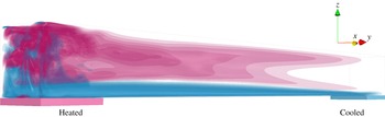
and the relative areas of the heated and cooled surfaces compared to the bottom area, see figure 1. Here
 $\unicode[STIX]{x1D708}$
denotes the kinematic viscosity,
 $\unicode[STIX]{x1D705}$
the thermal diffusivity,
 $\unicode[STIX]{x1D6FC}$
the isobaric thermal expansion coefficient of the fluid,
 $g$
the acceleration due to gravity,
 $L$
is the length and
 $H$
the height of the convection cell and
 $\unicode[STIX]{x1D6E5}\equiv (T_{+}-T_{-})$
with
 $T_{+}$
the temperature of the heated part of the bottom and
 $T_{-}$
the temperature of the cooled part of the bottom.
Sketch of an HC set-up together with the velocity
 $u_{y}$
in the horizontal
 $y$
-direction, as obtained in the direct numerical simulations of HC for
 $\mathit{Pr}=1$
,
 $\mathit{Ra}=10^{11}$
,
 $\unicode[STIX]{x1D6E4}=10$
. Pink colour reflects the flow away from the heated part of the bottom plate (
 $u_{y}>0$
) and blue corresponds to the flow away from the cooled part of the bottom (
 $u_{y}<0$
).

Convection cell configurations, or imposed BCs, are known to significantly influence the mean convective heat transport and momentum transport measured by the Nusselt number (
 $\mathit{Nu}$
) and Reynolds number (
 $\mathit{Re}$
), respectively (see, e.g. Grossmann & Lohse Reference Grossmann and Lohse2000; Daya & Ecke Reference Daya and Ecke2001; Gibert et al.
Reference Gibert, Pabiou, Chillà and Castaing2006; Song & Tong Reference Song and Tong2010; Boffetta & Ecke Reference Boffetta and Ecke2012; He et al.
Reference He, Funfschilling, Nobach, Bodenschatz and Ahlers2012; Stevens et al.
Reference Stevens, van der Poel, Grossmann and Lohse2013; Hassanzadeh, Chini & Doering Reference Hassanzadeh, Chini and Doering2014; Horn & Shishkina Reference Horn and Shishkina2015; Huang et al.
Reference Huang, Wang, Xi and Xia2015; Shishkina Reference Shishkina2016; Shishkina & Horn Reference Shishkina and Horn2016). How
 $\mathit{Nu}$
and
 $\mathit{Re}$
scales with
 $\mathit{Ra}$
and
 $\mathit{Pr}$
for different configurations is one of the main issues in investigations of thermally driven flows.
In Shishkina, Grossmann & Lohse (Reference Shishkina, Grossmann and Lohse2016) a theoretical model for heat and momentum transport scalings in HC was proposed, which is based on the ideas of Grossmann & Lohse (Reference Grossmann and Lohse2000, Reference Grossmann and Lohse2001) applied to HC flows. The model suggests multiple scaling regimes, including the Rossby (Reference Rossby1965) scaling for laminar flows and the ultimate scaling for fully turbulent flows (Siggers, Kerswell & Balmforth Reference Siggers, Kerswell and Balmforth2004). In particular, for laminar HC the scalings
 $$\begin{eqnarray}\displaystyle & \mathit{Re}\sim \mathit{Ra}^{2/5}\mathit{Pr}^{-4/5},\quad \mathit{Nu}\sim \mathit{Ra}^{1/5}\mathit{Pr}^{1/10} & \displaystyle\end{eqnarray}$$
for small
 $\mathit{Pr}$
with a transition to
 $$\begin{eqnarray}\displaystyle \mathit{Re}\sim \mathit{Ra}^{1/2}\mathit{Pr}^{-1},\quad \mathit{Nu}\sim \mathit{Ra}^{1/4}\mathit{Pr}^{0} & & \displaystyle\end{eqnarray}$$
for large
 $\mathit{Pr}$
were predicted. Here the Nusselt number is defined as
 $$\begin{eqnarray}\displaystyle & \displaystyle \mathit{Nu}\equiv -\frac{\langle \unicode[STIX]{x2202}T/\unicode[STIX]{x2202}z\rangle _{+}}{\unicode[STIX]{x1D6E5}/L}=\frac{\langle \unicode[STIX]{x2202}T/\unicode[STIX]{x2202}z\rangle _{-}}{\unicode[STIX]{x1D6E5}/L} & \displaystyle\end{eqnarray}$$
and the Reynolds number as
 $$\begin{eqnarray}\displaystyle & \mathit{Re}\equiv (\overline{\boldsymbol{u}\boldsymbol{\cdot }\boldsymbol{u}})^{1/2}L/\unicode[STIX]{x1D708}, & \displaystyle\end{eqnarray}$$
where
 $T$
is the temperature and
 $\boldsymbol{u}\equiv (u_{x},u_{y},u_{z})$
the velocity vector function,
 $z$
denotes the vertical direction,
 $\langle \cdot \rangle _{+}$
the averaging over the heated part of the bottom and in time,
 $\langle \cdot \rangle _{-}$
the averaging over the cooled part of the bottom and in time and the bar denotes the time and volume averages. The existence of the scaling regimes (1.4) and (1.5) was proved in numerical simulations of laminar HC by Shishkina & Wagner (Reference Shishkina and Wagner2016).
Another important issue in HC studies is the global flow structure, that is, the spatial distributions of the main flow characteristics like the temperature, velocity, kinetic energy, thermal and kinetic dissipation rates. In the present work we report
 $\mathit{Pr}$
- and
 $\mathit{Ra}$
-dependences of the global flow structures in HC, based on direct numerical simulations (DNS), and discuss how HC flows become transitional and turbulent for sufficiently large
 $\mathit{Ra}$
and
 $\unicode[STIX]{x1D6E4}$
. Apart from this, we also investigate the boundary layer (BL) contributions to the total thermal and kinetic dissipation rates in HC and show that for unsteady HC flows they gradually decrease with growing
 $\mathit{Ra}$
. This is consistent with the theoretical predictions from Shishkina et al. (Reference Shishkina, Grossmann and Lohse2016), where the dominance of the bulk contributions to the total thermal and kinetic dissipation rates is assumed in fully turbulent scaling regimes in HC.
2 Results
We consider the following equations in a Cartesian coordinate system
 $(x,y,z)\equiv (x_{1},x_{2},x_{3})$
, which describe an HC flow in Oberbeck–Boussinesq approximation:
 $$\begin{eqnarray}\displaystyle & \unicode[STIX]{x2202}\boldsymbol{u}/\unicode[STIX]{x2202}t+\boldsymbol{u}\boldsymbol{\cdot }\unicode[STIX]{x1D735}\boldsymbol{u}+\unicode[STIX]{x1D735}p=\unicode[STIX]{x1D708}\unicode[STIX]{x1D6FB}^{2}\boldsymbol{u}+\unicode[STIX]{x1D6FC}g\unicode[STIX]{x1D703}\boldsymbol{e}_{z}, & \displaystyle\end{eqnarray}$$
 $$\begin{eqnarray}\displaystyle & \unicode[STIX]{x2202}\unicode[STIX]{x1D703}/\unicode[STIX]{x2202}t+\boldsymbol{u}\boldsymbol{\cdot }\unicode[STIX]{x1D735}\unicode[STIX]{x1D703}=\unicode[STIX]{x1D705}\unicode[STIX]{x1D6FB}^{2}\unicode[STIX]{x1D703}, & \displaystyle\end{eqnarray}$$
 $$\begin{eqnarray}\displaystyle & \unicode[STIX]{x1D735}\boldsymbol{\cdot }\boldsymbol{u}=0, & \displaystyle\end{eqnarray}$$
where
 $p$
the kinetic pressure and
 $\boldsymbol{e}_{z}\equiv (0,0,1)^{\text{T}}$
. Further,
 $\unicode[STIX]{x1D703}$
is the reduced temperature,
 $\unicode[STIX]{x1D703}\equiv T-T_{m}$
with
 $T_{m}\equiv (T_{+}+T_{-})/2$
. On the domain boundaries no-slip BCs are considered,
 $\boldsymbol{u}=0$
. At the bottom heated part
 $S_{+}$
holds
 $\unicode[STIX]{x1D703}=\unicode[STIX]{x1D6E5}/2$
, while
 $\unicode[STIX]{x1D703}=-\unicode[STIX]{x1D6E5}/2$
on the cooled bottom part
 $S_{-}$
. At the rest of the bottom and at the top and side walls
 $\unicode[STIX]{x2202}\unicode[STIX]{x1D703}/\unicode[STIX]{x2202}\boldsymbol{n}=0$
holds with
 $\boldsymbol{n}$
the unit normal vector. The area
 $|S|$
of the bottom
 $S$
and the area
 $|S_{+}|$
of the heated part of the bottom are related as
 $|S|=\unicode[STIX]{x1D6E4}|S_{+}|$
, and the areas of the heated and cooled parts are equal,
 $|S_{+}|=|S_{-}|$
. Finally, the length, height and width of a parallelepiped computational domain are related as
 $\unicode[STIX]{x1D6E4}$
: 1 : 1 (see figure 1).
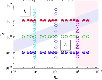
Sketch of the conducted DNS (symbols) and the phase diagram in an (
 $\mathit{Ra}$
,
 $\mathit{Pr}$
) plane for laminar regimes
 $\boldsymbol{I}_{\ell }$
and
 $\boldsymbol{I}_{\ell }^{\ast }$
, according to Shishkina et al. (Reference Shishkina, Grossmann and Lohse2016). Transition to turbulent regimes in HC is shown with the vertical pink stripe. The purple inclined stripe shows a transition from
 $\boldsymbol{I}_{\ell }$
to
 $\boldsymbol{I}_{\ell }^{\ast }$
with a slope
 $\mathit{Pr}\sim \mathit{Ra}^{1/2}$
. Different symbols reflect different DNS data sets, presented in figures 8 and 10.

For the system (2.1)–(2.3) the following holds:
 $$\begin{eqnarray}\displaystyle & \overline{u_{z}\unicode[STIX]{x1D703}}=\unicode[STIX]{x1D705}(\langle \unicode[STIX]{x1D703}\rangle _{z=H}-\langle \unicode[STIX]{x1D703}\rangle _{z=0})/H=B(\unicode[STIX]{x1D6E4}-1)\unicode[STIX]{x1D705}\unicode[STIX]{x1D6E5}/L. & \displaystyle\end{eqnarray}$$
Here
 $\langle \cdot \rangle _{z}$
denotes the averaging in time and over a horizontal cross-section at the height
 $z$
and
 $B$
is a certain constant,
 $0<B\leqslant 1$
. The constant
 $B$
is equal to 1 only if
 $\langle \unicode[STIX]{x1D703}\rangle _{z=H}=\unicode[STIX]{x1D6E5}/2$
and the temperature of the adiabatic part of the bottom equals
 $(-\unicode[STIX]{x1D6E5}/2)$
. From (2.1) and (2.4) it follows, in particular, that
 $$\begin{eqnarray}\displaystyle & \overline{\unicode[STIX]{x1D716}_{u}}=\unicode[STIX]{x1D6FC}g\overline{u_{z}\unicode[STIX]{x1D703}}=B(\unicode[STIX]{x1D6E4}-1)\unicode[STIX]{x1D6FC}g\unicode[STIX]{x1D705}\unicode[STIX]{x1D6E5}L^{-1}=\unicode[STIX]{x1D708}^{3}L^{-4}B(\unicode[STIX]{x1D6E4}-1)\mathit{Ra}\,\mathit{Pr}^{-2}. & \displaystyle\end{eqnarray}$$
Here
 $\unicode[STIX]{x1D716}_{u}\equiv \unicode[STIX]{x1D708}\sum _{i,j}(\unicode[STIX]{x2202}u_{j}/\unicode[STIX]{x2202}x_{i})^{2}$
is the kinetic dissipation rate. Note that in RBC in a similar equality an extra factor
 $(\mathit{Nu}-1)$
is present in the right-hand side. Therefore, for the same
 $\mathit{Ra}$
and
 $\mathit{Pr}$
, the mean kinetic dissipation rate in HC is smaller than in RBC. All this leads to generally smaller exponents in the
 $\mathit{Nu}$
versus
 $\mathit{Ra}$
scalings, see details in Shishkina et al. (Reference Shishkina, Grossmann and Lohse2016).
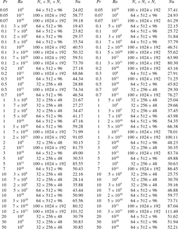
Parameters of the conducted DNS of HC:
 $\mathit{Pr}$
,
 $\mathit{Ra}$
and the number of nodes in each direction of the computational mesh,
 $N_{x}\times N_{y}\times N_{z}$
, together with the obtained
 $\mathit{Nu}$
.

In the DNS we use the finite-volume code goldfish and investigate HC flows for
 $\unicode[STIX]{x1D6E4}=10$
and
 $\mathit{Ra}$
from
 $3\times 10^{8}$
to
 $3\times 10^{11}$
and
 $\mathit{Pr}$
from 0.05–50, i.e. more than 3 decades in
 $\mathit{Ra}$
and
 $\mathit{Pr}$
, see Shishkina & Wagner (Reference Shishkina and Wagner2016). A sketch of the conducted DNS and of the phase diagram in an (
 $\mathit{Ra}$
,
 $\mathit{Pr}$
) plane are presented in figure 2. Details on the simulations are given in table 1. The computational meshes in the directions
 $(x,y,z)$
range from
 $32\times 256\times 48$
for small
 $\mathit{Ra}$
and large
 $\mathit{Pr}$
to
 $100\times 1024\times 192$
nodes for large
 $\mathit{Ra}$
and small
 $\mathit{Pr}$
. They are sufficiently fine to resolve the Kolmogorov microscale
 $\unicode[STIX]{x1D702}_{K}$
and Batchelor microscale
 $\unicode[STIX]{x1D702}_{B}$
in the DNS (Shishkina et al.
Reference Shishkina, Stevens, Grossmann and Lohse2010),
 $$\begin{eqnarray}\displaystyle & \unicode[STIX]{x1D702}_{K}\equiv (\unicode[STIX]{x1D708}^{3}/\unicode[STIX]{x1D716}_{u})^{1/4},\quad \unicode[STIX]{x1D702}_{B}\equiv (\unicode[STIX]{x1D708}\unicode[STIX]{x1D705}^{2}/\unicode[STIX]{x1D716}_{u})^{1/4}. & \displaystyle\end{eqnarray}$$
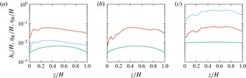
In particular, in figure 3 one can see the mesh spacing in the vertical
 $z$
-direction (
 $h_{z}$
) which is plotted against the Kolmogorov microscale (
 $\unicode[STIX]{x1D702}_{K}$
) and Batchelor microscale (
 $\unicode[STIX]{x1D702}_{B}$
), averaged in the horizontal directions
 $x$
and
 $y$
.
Mesh spacing in the vertical
 $z$
-direction (
 $h_{z}$
, green) compared to the Kolmogorov microscale (
 $\unicode[STIX]{x1D702}_{K}$
, blue) and Batchelor microscale (
 $\unicode[STIX]{x1D702}_{B}$
, red), averaged in the horizontal directions
 $x$
and
 $y$
, for (a)
 $\mathit{Pr}=0.05$
and
 $\mathit{Ra}=10^{10}$
, (b)
 $\mathit{Pr}=1$
and
 $\mathit{Ra}=2\times 10^{11}$
and (c)
 $\mathit{Pr}=50$
and
 $\mathit{Ra}=10^{10}$
. In (b) for
 $\mathit{Pr}=1$
holds
 $\unicode[STIX]{x1D702}_{K}=\unicode[STIX]{x1D702}_{B}$
and the corresponding curves coincide.

From (2.5) and (2.6) if follows that the mean Kolmogorov microscale in HC scales with
 $\mathit{Ra}$
and
 $\mathit{Pr}$
as
 $$\begin{eqnarray}\displaystyle & \overline{\unicode[STIX]{x1D702}_{K}}\sim \mathit{Pr}^{1/2}\mathit{Ra}^{-1/4}, & \displaystyle\end{eqnarray}$$
while the mean Batchelor microscale scales as
 $$\begin{eqnarray}\displaystyle & \overline{\unicode[STIX]{x1D702}_{B}}\sim \mathit{Pr}^{0}\mathit{Ra}^{-1/4}, & \displaystyle\end{eqnarray}$$
i.e. is independent from
 $\mathit{Pr}$
. Thus, to study HC for a fixed
 $\mathit{Ra}$
in the DNS, one generally needs much finer meshes for
 $\mathit{Pr}\ll 1$
than is required in the case of
 $\mathit{Pr}\sim 1$
or
 $\mathit{Pr}\gg 1$
. Although for
 $\mathit{Pr}\gg 1$
one can use similar meshes as for
 $\mathit{Pr}\sim 1$
, the DNS are generally slower for
 $\mathit{Pr}\gg 1$
, since a finer time stepping is needed in the case
 $\mathit{Pr}\gg 1$
, due to the numerical von Neumann stability (Shishkina Reference Shishkina2007) of the used time discretization schemes.
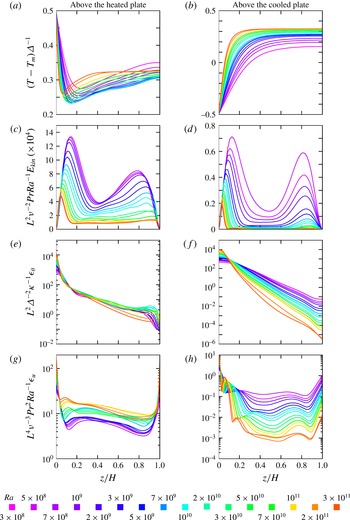
Vertical profiles of the normalized (a,b) temperature, (c,d) kinetic energy, (e,f) thermal dissipation rate and (g,h) kinetic dissipation rate, as obtained in the DNS for
 $\mathit{Pr}=1$
and different
 $\mathit{Ra}$
(the colour scale is on the bottom of the figure). All profiles are averaged in time and in the
 $x$
-direction, and additionally either above the heated part of the bottom,
 $0\leqslant y/L\leqslant 0.1$
(a,c,e,g), or above the cooled part of the bottom,
 $0.9\leqslant y/L\leqslant 1$
(b,d,f,h).

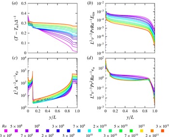
Horizontal profiles (along the HC cell) of the normalized (a) temperature, (b) kinetic energy, (c) thermal dissipation rate and (d) kinetic dissipation rate, as obtained in the DNS for
 $\mathit{Pr}=1$
and different
 $\mathit{Ra}$
(the colour scale is on the bottom of the figure). All profiles are averaged in time and in the
 $x$
- and
 $z$
-directions.

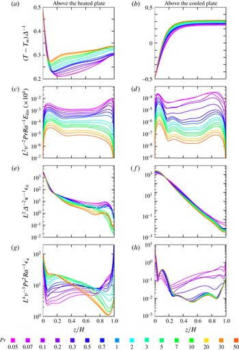
Vertical profiles of the normalized (a,b) temperature, (c,d) kinetic energy, (e,f) thermal dissipation rate and (g,h) kinetic dissipation rate, as obtained in the DNS for
 $\mathit{Ra}=10^{10}$
and different
 $\mathit{Pr}$
(the colour scale is on the bottom of the figure). All profiles are averaged in time and in the
 $x$
-direction, and additionally either above the heated part of the bottom,
 $0\leqslant y/L\leqslant 0.1$
(a,c,e,g), or above the cooled part of the bottom,
 $0.9\leqslant y/L\leqslant 1$
(b,d,f,h).

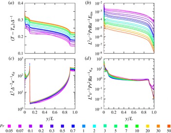
Horizontal profiles (along the HC cell) of the normalized (a) temperature, (b) kinetic energy, (c) thermal dissipation rate and (d) kinetic dissipation rate, as obtained in the DNS for
 $\mathit{Ra}=10^{10}$
and different
 $\mathit{Pr}$
(the colour scale is on the bottom of the figure). All profiles are averaged in time and in the
 $x$
- and
 $z$
-directions.

In figures 4 and 5 the time-averaged profiles of the temperature
 $T$
, kinetic energy
 $E_{kin}\equiv \boldsymbol{u}\boldsymbol{\cdot }\boldsymbol{u}$
, thermal dissipation rate
 $\unicode[STIX]{x1D716}_{\unicode[STIX]{x1D703}}\equiv \unicode[STIX]{x1D705}\sum _{i}(\unicode[STIX]{x2202}T/\unicode[STIX]{x2202}x_{i})^{2}$
and kinetic dissipation rate
 $\unicode[STIX]{x1D716}_{u}$
are presented for different
 $\mathit{Ra}$
and
 $\mathit{Pr}=1$
, while in figures 6 and 7 similar dependences are shown for a fixed
 $\mathit{Ra}=10^{10}$
and different
 $\mathit{Pr}$
. The profiles, averaged in the
 $x$
-direction and
 $0\leqslant y/L\leqslant 0.1$
, i.e. above the heated part of the bottom, are presented in the left columns of figures 4 and 6, while those, averaged in the
 $x$
-direction and
 $0.9\leqslant y/L\leqslant 1$
, i.e. above the cooled part of the bottom, are presented in the right columns of these figures. These profiles are functions of the distance
 $z$
from the bottom. Figures 5 and 7 present the profiles that depend on the coordinate
 $y$
and are averaged in the
 $x$
and
 $z$
directions. They show how the main flow characteristics change while moving from one vertical wall, which is attached to the heated part of the bottom, to the opposite vertical wall, which is attached to the cooled part of the bottom.
The DNS show that the vertical temperature profiles above the heated plate (figures 4
a and 6
a) are non-monotonic functions of
 $z$
and have their minimum at a certain distance from the bottom. We define the thermal BL thickness
 $\unicode[STIX]{x1D706}_{\unicode[STIX]{x1D703}}$
as the distance from the bottom, at which the global minimum of the temperature profile as in figure 4(a) is obtained. Obviously, the values of
 $\unicode[STIX]{x1D706}_{\unicode[STIX]{x1D703}}$
are smaller for larger
 $\mathit{Ra}$
(figure 4
a) and larger
 $\mathit{Pr}$
(figure 6
a).
For small
 $\mathit{Pr}$
the mixing in the core part of the domain is more effective and therefore, the drop of the temperature from that at the heated bottom (
 $z=0$
) to that at half height (
 $z=H/2$
) is larger for smaller
 $\mathit{Pr}$
(figure 6
a). At
 $z=0$
the slopes of the temperature profiles at the heated part of the bottom are steeper for larger
 $\mathit{Ra}$
(figure 4
a) and almost unaffected by
 $\mathit{Pr}$
(figure 6
a). This is consistent with the scaling
 $\mathit{Nu}\sim \mathit{Ra}^{1/4}\mathit{Pr}^{0}$
for laminar HC flows with
 $\mathit{Pr}\gtrsim 0.1$
(Shishkina & Wagner Reference Shishkina and Wagner2016). Since the Nusselt number measured at the heated part of the bottom is the same as that at the cooled part, the slopes of the temperature profiles at the cooled part of the bottom behave similarly to those at the heated part: they are steeper for larger
 $\mathit{Ra}$
(figure 4
b) and only weakly depend on
 $\mathit{Pr}$
(figure 6
b). In the upper region of the convection cell, above the cooled bottom part, the temperature is generally larger for larger
 $\mathit{Ra}$
(figure 4
b) and larger
 $\mathit{Pr}$
(figure 6
b). In the bulk, the temperature profiles along the cell are almost linear functions of
 $y$
(figures 5
a and 7
a), those slopes, being gentler for larger
 $\mathit{Ra}$
(figure 5
a), are mainly determined by
 $\mathit{Pr}$
(figure 7
a). Generally, the mean temperature of the bulk is larger for larger
 $\mathit{Ra}$
(figure 5
a) and
 $\mathit{Pr}$
(figure 7
a).
The kinetic energy profile in the vertical
 $z$
direction above the heated plate (figures 4
c and 6
c), is also a non-monotonic function of
 $z$
. A point of its local maximum, which is closest to the bottom, determines the thickness
 $\unicode[STIX]{x1D706}_{u}$
of the bottom viscous BL. Analogously, the thickness of the top viscous BL is defined as the distance from the top of the convection cell to the nearest point of maximum of the kinetic energy. One can see that for a fixed
 $\mathit{Pr}$
, the slopes of
 $(L/\unicode[STIX]{x1D708})^{2}\mathit{Pr}\mathit{Ra}^{-1}E_{kin}$
at the hot plate (figure 4
c) and at the cold plate (figure 4
d) are independent of
 $\mathit{Ra}$
, but the absolute values of the maxima are determined by
 $\mathit{Ra}$
, which are smaller for larger
 $\mathit{Ra}$
. This means that with growing
 $\mathit{Ra}$
, the magnitude of the maximum kinetic energy above the plates scales slower than
 ${\sim}\mathit{Ra}$
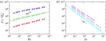
. This is in conformity with the scaling with the Rayleigh number of the total time- and volume-averaged kinetic energy
 $\overline{E_{kin}}\sim (\unicode[STIX]{x1D708}/L)^{2}\mathit{Ra}^{0.68}$
, see figure 8. The thicknesses of the viscous BLs are generally larger for smaller
 $\mathit{Ra}$
(figures 4
c and 4
d) and larger
 $\mathit{Pr}$
(figures 6
c and 6
d). In the bulk
 $(L/\unicode[STIX]{x1D708})^{2}\mathit{Pr}\mathit{Ra}^{-1}E_{kin}$
decreases with increasing
 $y$
, i.e. while moving from the hot plate toward the cold plate, and its absolute values are generally smaller for larger
 $\mathit{Ra}$
and
 $\mathit{Pr}$
(figures 5
b and 7
b).
(a)
 $\mathit{Ra}$
-dependences and (b)
 $\mathit{Pr}$
-dependences of the normalized time- and volume-averaged kinetic energy, as obtained in the DNS for (a)
 $Pr=0.1$
(lower-half-filled circles),
 $Pr=1$
(open circles),
 $Pr=10$
(upper-half-filled circles) and for (b)
 $Ra=10^{9}$
(down-pointing triangles),
 $Ra=10^{10}$
(diamonds) and
 $Ra=10^{11}$
(up-pointing triangles).

(a)
 $\mathit{Ra}$
-dependences for
 $\mathit{Pr}=1$
and (b)
 $\mathit{Pr}$
-dependences for
 $\mathit{Ra}=10^{10}$
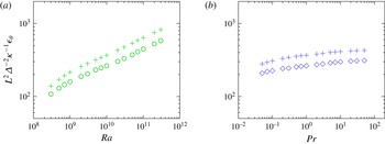
of the normalized thermal dissipation rate
 $\unicode[STIX]{x1D716}_{\unicode[STIX]{x1D703}}$
(circles and diamonds), averaged in time and in the
 $x$
- and
 $z$
-directions and evaluated at
 $y=0.9L$
, i.e. at the boundary between the cold and adiabatic parts of the bottom. Pluses in (a,b) show the corresponding estimates
 $(L/\unicode[STIX]{x1D6E5})^{2}(\unicode[STIX]{x2202}T/\unicode[STIX]{x2202}z|_{z=0})^{2}(\unicode[STIX]{x1D706}_{\unicode[STIX]{x1D703},c}/H)$
, averaged in time and in the
 $x$
-direction and above the cooled part of the bottom,
 $0.9\leqslant y/L\leqslant 1$
. Here
 $\unicode[STIX]{x1D706}_{\unicode[STIX]{x1D703},c}$
is the thickness of the thermal BL at the cooled bottom plate, evaluated with the slope method, equation (2.9).

Normalized thermal dissipation rate
 $(L/\unicode[STIX]{x1D6E5})^{2}\unicode[STIX]{x1D705}^{-1}\unicode[STIX]{x1D716}_{\unicode[STIX]{x1D703}}$
decreases monotonically and fast with increasing distance from the bottom (figures 4
e, 4
f, 6
e and 6
f). Its slope is steeper for larger
 $\mathit{Ra}$
. The behaviour of
 $\unicode[STIX]{x1D716}_{\unicode[STIX]{x1D703}}$
along the cell is much more complicated (figures 5
c and 7
c) and is determined by the processes close to the bottom. Figure 1 helps to understand the global flow structure in HC and the corresponding distribution of
 $\unicode[STIX]{x1D716}_{\unicode[STIX]{x1D703}}$
. Close to the bottom the flow goes from the right to the left, i.e. from the cooled part towards the heated part of the bottom. Above the cooled plate,
 $\unicode[STIX]{x1D716}_{\unicode[STIX]{x1D703}}$
is constantly large due to the presence of the thermal BL. Since at the adiabatic central piece of the bottom there is no thermal BL, the thermal dissipation rate gradually decreases while moving from the right to the left. At
 $y/L=0.1$
, where the adiabatic bottom plate meets the heated plate,
 $\unicode[STIX]{x1D716}_{\unicode[STIX]{x1D703}}$
has a sudden peak. Its origin is caused by an invasion of the lower cold flow of the hot thermal boundary layer, which leads to very large temperature gradients. As expected, above the heated part of the bottom (
 $0\leqslant y/L\leqslant 0.1$
) and above the cooled part (
 $0.9\leqslant y/L\leqslant 1$
), the thermal dissipation rate
 $\unicode[STIX]{x1D716}_{\unicode[STIX]{x1D703}}$
is larger for larger
 $\mathit{Ra}$
(figure 5
c).
Note that above the cooled part of the bottom, the HC flows are laminar for the studied
 $\mathit{Ra}$
-range. Therefore, the thermal dissipation rate, averaged in time and in the
 $x$
- and
 $z$
-directions, is mainly determined by the temperature gradients at the bottom and the thickness of the thermal BL at the cooled bottom plate,
 $\unicode[STIX]{x1D706}_{\unicode[STIX]{x1D703},c}$
, evaluated with the slope method, see figure 9. More precisely,
 $\unicode[STIX]{x1D706}_{\unicode[STIX]{x1D703},c}$
is evaluated from
 $$\begin{eqnarray}\displaystyle \unicode[STIX]{x1D706}_{\unicode[STIX]{x1D703},c}\langle \unicode[STIX]{x2202}T/\unicode[STIX]{x2202}z|_{z=0}\rangle _{-}=T_{-}^{\ast }-T_{-}, & & \displaystyle\end{eqnarray}$$
where
 $T_{-}^{\ast }$
is the temperature at the top plate (
 $z=H$
), averaged in time, in the
 $x$
-direction and above the cooled part of the bottom,
 $0.9\leqslant y/L\leqslant 1$
.
The viscous dissipation rate
 $\unicode[STIX]{x1D716}_{u}$
generally decreases with increasing
 $y$
, i.e. while moving along the cell from the heated plate towards the cooled one (figures 5
d and 7
d). It is large at the rigid top and bottom walls (figures 4
g and 6
g), while having its absolute minimum close to the bottom if
 $\mathit{Pr}$
is small or close to the top if
 $\mathit{Pr}$
is large (figure 6
g).
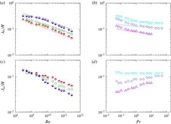
In figure 10 one can see the dependences on
 $\mathit{Ra}$
and
 $\mathit{Pr}$
of the thicknesses of the thermal and viscous BLs, attached to the heated part of the bottom. Obviously,
 $\unicode[STIX]{x1D706}_{u}$
and
 $\unicode[STIX]{x1D706}_{\unicode[STIX]{x1D703}}$
decrease with increasing
 $\mathit{Ra}$
(figure 10
a,c). Since
 $\unicode[STIX]{x1D706}_{\unicode[STIX]{x1D703}}$
is defined by the point of minimum of the vertical temperature profiles above the heated plate (figures 4
a and 6
a) and not using the slope method, the
 $\mathit{Pr}$
- and
 $\mathit{Ra}$
-dependences of
 $\unicode[STIX]{x1D706}_{\unicode[STIX]{x1D703}}$
do not replicate those of
 $\propto \mathit{Nu}^{-1}$
(cf. symbols and dashed lines in figure 10
a,b), but in general
 $\unicode[STIX]{x1D706}_{\unicode[STIX]{x1D703}}$
and
 $\mathit{Nu}^{-1}$
behave very similar. Here the Nusselt number is evaluated at the heated part of the bottom plate, according to the definition of
 $\mathit{Nu}$
(1.6). As expected, for a fixed
 $\mathit{Ra}$
,
 $\unicode[STIX]{x1D706}_{\unicode[STIX]{x1D703}}$
decreases and
 $\unicode[STIX]{x1D706}_{u}$
increases with growing
 $\mathit{Pr}$
(figure 10
b,d).
(a,c)
 $\mathit{Ra}$
-dependences and (b,d)
 $\mathit{Pr}$
-dependences of the normalized time-averaged thicknesses of (a,b) the thermal BLs and (c,d) the viscous BLs above the heated part of the bottom, as obtained in the DNS for (a,c)
 $\mathit{Pr}=0.1$
(lower-half-filled circles),
 $\mathit{Pr}=1$
(open circles),
 $\mathit{Pr}=10$
(upper-half-filled circles) and for (b,d)
 $\mathit{Ra}=10^{9}$
(down-pointing triangles),
 $\mathit{Ra}=10^{10}$
(diamonds) and
 $\mathit{Ra}=10^{11}$
(up-pointing triangles). Dash lines in (a,b) show the corresponding fits
 $\propto \mathit{Nu}^{-1}$
, where
 $\mathit{Nu}$
is evaluated at the heated part of the bottom, according to its definition (1.6).

One can see that with varying Rayleigh number and Prandtl number, the tendencies in the global flow structures changes are similar in the cases of HC and RBC. Thus, the flows are more fluctuating with growing
 $\mathit{Ra}$
and decreasing
 $\mathit{Pr}$
in both cases. The thicknesses of the boundary layers decrease with growing
 $\mathit{Ra}$
and the balance of the thermal to viscous BL thicknesses is determined by
 $\mathit{Pr}$
in a similar way, in HC as well as in RBC. Although RBC and HC flows are similar to a certain extent, there are several very important differences between these flows. Below we highlight some of the features of the HC flow structures that differ them from the RBC ones.
It is well known that for sufficiently large
 $\mathit{Ra}$
, a RBC flow within the Oberbeck–Boussinesq approximation is convectively unstable in the whole domain. In contrast to this, in HC, also under the Oberbeck–Boussinesq approximation, there always exists a region in the convection cell, where the flow is convectively stable. This is a region above the cooled and adiabatic parts of the domain, see figure 1. As a result, in HC a more fluctuating flow develops above the heated plate compared to that above the cooled plate, while in RBC one observes symmetry with this respect.
Further, in HC the magnitudes of the kinetic energy and viscous dissipation rates near the heated and cooled plates are very different, being significantly larger near the heated plate, see figures 4(c,d,g,h) and 6(c,d,g,h). The distributions of the kinetic energy, thermal and viscous dissipation rates along the HC cell, i.e. along the imposed temperature gradient, are not symmetric with respect to the vertical plane located at a half-distance between the heated and cooled parts of the bottom (
 $y=L/2$
), see figures 5(b–d) and 7(b–d). Contrary to that, in RBC the distributions of these quantities along the imposed temperature gradient, i.e. along the vertical direction
 $z$
, are symmetric with respect to a plane located at a half-distance between the heated bottom and cooled top (
 $z=H/2$
). Moreover, the distribution of the thermal dissipation rate in the
 $y$
-direction in HC has several extrema and a sudden peak at the boundary between the heated and adiabatic parts of the bottom, while the corresponding distribution in RBC is smooth, having its maxima at the isothermal walls.
Asymmetry also takes place in the temperature and velocity distributions in HC. Thus, in the largest part of the HC cell the fluid moves in the direction from the heated bottom plate to the cooled one and the fluid with the temperature larger than the arithmetic mean of the temperature of the heated and cooled bottom plates occupies more than a half of the HC cell volume. Generally, the time- and volume-averaged temperature of the HC flow is larger than this arithmetic mean, being larger for larger
 $\mathit{Pr}$
and
 $\mathit{Ra}$
, see figures 5(a) and 7(a). Opposite to this, in Oberbeck–Boussinesq RBC, the fluid with the temperature larger than the arithmetic mean of the top and bottom temperatures occupies on average a half of the RBC cell.
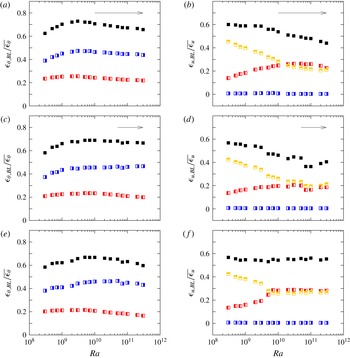
Thermal BL contributions (
 $\unicode[STIX]{x1D716}_{\unicode[STIX]{x1D703},\text{BL}}$
) and viscous BL contributions (
 $\unicode[STIX]{x1D716}_{u,\text{BL}}$
) to the total time- and volume-averaged (a,c,e) thermal dissipation rate
 $\overline{\unicode[STIX]{x1D716}_{\unicode[STIX]{x1D703}}}$
and (b,d,f) viscous dissipation rate
 $\overline{\unicode[STIX]{x1D716}_{u}}$
, as obtained in the DNS for (a,b)
 $\mathit{Pr}=0.1$
, (c,d)
 $\mathit{Pr}=1$
and (e,f)
 $\mathit{Pr}=10$
and different
 $\mathit{Ra}$
. Red left-half-filled squares: contributions from (a,c,e) the thermal BL or (b,d,f) the top and bottom viscous BLs above the heated part of the bottom,
 $0\leqslant y/L\leqslant 0.1$
. Blue right-half-filled squares: contributions from (a,c,e) the thermal BL or (b,d,f) the top and bottom viscous BLs above the cooled part of the bottom,
 $0.9\leqslant y/L\leqslant 1$
. Yellow upper-half-filled squares: (b,d,f) contributions from the top and bottom viscous BLs above the middle adiabatic part of the bottom,
 $0.1<y/L<0.9$
. Black filled squares: contributions from (a,c,e) the whole thermal BL or (b,d,f) from the whole top and bottom viscous BLs. Arrows show the regions, where the HC flows are unsteady.

3 Discussion
Above we have described the global flow structures in horizontal convection, based on the DNS for
 $\unicode[STIX]{x1D6E4}=10$
and
 $\mathit{Ra}$
from
 $3\times 10^{8}$
to
 $3\times 10^{11}$
and
 $\mathit{Pr}$
from 0.05 to 50. The HC flows above the heated part of the domain are convectively unstable. For sufficiently high
 $\mathit{Ra}$
this leads to the development of a transitional and later on of a turbulent flow in this region. In contrast to this, the rest (largest) part of the domain remains convectively stable. The region above the adiabatic bottom part and close to the heated part is disturbed by eddies developed in the region above the heated plate and the induced waves propagate in the core part of the domain. Further, the upwind flow above the heated part of the domain pushes the fluid in the upper region of the HC cell towards the cooled region. As a result, two horizontal flows along the convection cell develop, which are a warm fluid in the upper region of the cell that flows towards the cooled region, and a cooled fluid in the near the bottom region that flows towards the heated bottom part (see figure 1
a). With increasing
 $\mathit{Ra}$
these induced shear flows become stronger.
Although for the studied combinations of
 $\mathit{Ra}$
and
 $\mathit{Pr}$
, the HC flows are found to be laminar in the region above the adiabatic and cooled parts of the bottom, we can expect the development of a turbulent flow also there, for sufficiently high
 $\mathit{Ra}$
, by the following reasons. The upper warmer and lower colder fluid layers shear against each other, which leads to the Kelvin–Helmholtz instability at the interface of these two fluid layers. Such a two-layer shear flow is known to be unconditionally unstable. Around the interface of these two fluid layers, the interfacial waves induce flow perturbations, which form an internal mixing zone. The height of this zone is of the order of the wavelength of the longest unstable interfacial wave, which is proportional to the squared relative velocity of the two-layer shear flow (see, e.g. Cushman-Roisin & Beckers Reference Cushman-Roisin and Beckers2011). Since this velocity (or
 $\mathit{Re}$
) gradually increases with increasing
 $\mathit{Ra}$
, for sufficiently large
 $\mathit{Ra}$
and
 $\unicode[STIX]{x1D6E4}$
, a turbulent mixing zone can develop, the vertical extent of which is of the order of the height of the HC cell. In small-
 $\mathit{Pr}$
(less viscous) fluids we can expect transition to turbulence in HC for smaller
 $\mathit{Ra}$
than in the case of large-
 $\mathit{Pr}$
fluids.
With developing turbulent processes, as
 $\mathit{Ra}$
increases, the bulk contributions to the time- and volume-averaged dissipation rates also increase. This is supported by the DNS results presented in figure 11, where the BL contributions to the total
 $\unicode[STIX]{x1D716}_{\unicode[STIX]{x1D703}}$
and
 $\unicode[STIX]{x1D716}_{u}$
are shown. One can see that with growing
 $\mathit{Ra}$
, the BL contributions to the total
 $\unicode[STIX]{x1D716}_{\unicode[STIX]{x1D703}}$
and
 $\unicode[STIX]{x1D716}_{u}$
gradually decrease, as soon as the HC flows are unsteady, although the absolute values of the thermal and viscous dissipation rates at the heated plate increase with
 $\mathit{Ra}$
(figures 4
e and 4
g). From this one expects a dominance of the bulk contributions to
 $\unicode[STIX]{x1D716}_{\unicode[STIX]{x1D703}}$
and
 $\unicode[STIX]{x1D716}_{u}$
for sufficiently large
 $\mathit{Ra}$
and, hence, the scalings of
 $\mathit{Nu}$
and
 $\mathit{Re}$
with
 $\mathit{Ra}$
and
 $\mathit{Pr}$
as proposed in Shishkina et al. (Reference Shishkina, Grossmann and Lohse2016) for the turbulent regimes. Further numerical and experimental studies are needed to investigate in detail transition to turbulence in horizontal convection.
Acknowledgements
O.S. is grateful to G. Ahlers, E. Bodenschatz, E. Ching, M. Emran, L. Gizon, S. Grossmann, X. He, S. Horn, D. Lohse, S. Wagner, S. Weiss and K.-Q. Xia for useful discussions and acknowledges Leibniz Supercomputing Centre (LRZ) for providing computing time and the Deutsche Forschungsgemeinschaft (DFG) for financial support under the grant Sh405/4 – Heisenberg fellowship.