2.1 LNS

The first linear model is obtained by first substituting a Reynolds decomposition into the Navier–Stokes equations and then subtracting the mean equations, which gives

(2.2) $$\begin{eqnarray}\frac{\unicode[STIX]{x2202}\boldsymbol{u}}{\unicode[STIX]{x2202}t}+(\boldsymbol{U}\boldsymbol{\cdot }\unicode[STIX]{x1D735})\boldsymbol{u}+(\boldsymbol{u}\boldsymbol{\cdot }\unicode[STIX]{x1D735})\boldsymbol{U}+\unicode[STIX]{x1D735}\boldsymbol{p}-\frac{1}{Re_{\unicode[STIX]{x1D70F}}}\unicode[STIX]{x1D6FB}^{2}\boldsymbol{u}=\boldsymbol{d}_{LNS},\quad \unicode[STIX]{x1D735}\boldsymbol{\cdot }\boldsymbol{u}=0,\end{eqnarray}$$

where $\boldsymbol{U}=(U(z),0,0)$ is the mean velocity profile that is obtained using (2.1) and $\boldsymbol{u}=(u,v,w)$ denotes the fluctuations of velocity from the mean. Following McKeon & Sharma (Reference McKeon and Sharma2010), the nonlinear terms are represented by a disturbance term $\boldsymbol{d}_{LNS}=-\boldsymbol{u}\boldsymbol{\cdot }\unicode[STIX]{x1D735}\boldsymbol{u}+\overline{\boldsymbol{u}\boldsymbol{\cdot }\unicode[STIX]{x1D735}\boldsymbol{u}}$ . Here, $\boldsymbol{d}_{LNS}$ is assumed to be stochastic and white-in-time (Hwang & Cossu Reference Hwang and Cossu2010a ).

2.2 eLNS

The second linear model is obtained by substituting into the Navier–Stokes equations a triple decomposition of the velocity field as $\tilde{\boldsymbol{u}}=\boldsymbol{U}+\boldsymbol{u}+\boldsymbol{u}^{\prime }$ , where $\boldsymbol{U}$ as before is the mean velocity, the term $\boldsymbol{u}$ denotes the organised motions and $\boldsymbol{u}^{\prime }$ represents the turbulent velocity fluctuations (Reynolds & Hussain Reference Reynolds and Hussain1972; Del Álamo & Jiménez Reference Del Álamo and Jiménez2006; Pujals et al. Reference Pujals, García-Villalba, Cossu and Depardon2009; Hwang & Cossu Reference Hwang and Cossu2010b ). The Cess (Reference Cess1958) eddy viscosity profile (2.1) is used to model the terms that are quadratic in $\boldsymbol{u}^{\prime }$ . This model can be written as

(2.3) $$\begin{eqnarray}\frac{\unicode[STIX]{x2202}\boldsymbol{u}}{\unicode[STIX]{x2202}t}+(\boldsymbol{U}\boldsymbol{\cdot }\unicode[STIX]{x1D735})\boldsymbol{u}+(\boldsymbol{u}\boldsymbol{\cdot }\unicode[STIX]{x1D735})\boldsymbol{U}+\unicode[STIX]{x1D735}\boldsymbol{p}-\unicode[STIX]{x1D735}\boldsymbol{\cdot }\left[\frac{\unicode[STIX]{x1D708}_{T}(z)}{\unicode[STIX]{x1D708}}(\unicode[STIX]{x1D735}\boldsymbol{u}+\unicode[STIX]{x1D735}\boldsymbol{u}^{T})\right]=\boldsymbol{d}_{eLNS},\quad \unicode[STIX]{x1D735}\boldsymbol{\cdot }\boldsymbol{u}=0.\end{eqnarray}$$

The mean velocity profile is again obtained using (2.1). Additionally, (2.1) also provides the eddy viscosity profile $\unicode[STIX]{x1D708}_{T}(z)$ required for (2.3). The term $\boldsymbol{d}_{eLNS}$ represents the forcing, but is defined using $\boldsymbol{u}$ obtained from the triple decomposition of the velocity field. As before, $\boldsymbol{d}_{eLNS}$ is assumed to be stochastic and white-in-time.

2.3 Orr–Sommerfeld-Squire form

The models in (2.2) and (2.3) can now be written in the Orr–Sommerfeld-Squire form. A 2-D Fourier transformation of $\boldsymbol{u}$ and $\boldsymbol{d}$ along the homogeneous streamwise and spanwise directions gives the respective Fourier coefficients $\hat{\boldsymbol{u}}(z,t;k_{x},k_{y})=(\hat{u} ,\hat{v},{\hat{w}})$ and $\hat{\boldsymbol{d}}(z,t;k_{x},k_{y})=(\hat{d_{x}},\hat{d_{y}},\hat{d_{z}})$ . Here ( $k_{x},k_{y}$ ) are the streamwise and spanwise wavenumbers and ( $\unicode[STIX]{x1D706}_{x},\unicode[STIX]{x1D706}_{y}$ ) the corresponding wavelengths. In terms of these Fourier coefficients, the Orr–Sommerfeld-Squire form of the models (2.2) and (2.3) is (Del Álamo & Jiménez Reference Del Álamo and Jiménez2006; Hwang & Cossu Reference Hwang and Cossu2010b )

(2.4) $$\begin{eqnarray}\displaystyle \left.\begin{array}{@{}c@{}}\displaystyle \dot{\hat{\boldsymbol{q}}}=\unicode[STIX]{x1D63C}\hat{\boldsymbol{q}}+\unicode[STIX]{x1D63D}\hat{\boldsymbol{d}},\\ \displaystyle \hat{\boldsymbol{u}}=\unicode[STIX]{x1D63E}\hat{\boldsymbol{q}},\end{array}\right\} & & \displaystyle\end{eqnarray}$$

where the definitions of the matrices $\unicode[STIX]{x1D63C}$ , $\unicode[STIX]{x1D63D}$ and $\unicode[STIX]{x1D63E}$ for both LNS and eLNS are given in appendix A. The vector $\hat{\boldsymbol{q}}=({\hat{w}},\hat{\unicode[STIX]{x1D702}})$ is formed with Fourier coefficients of the wall-normal velocity and wall-normal vorticity. The boundary conditions are enforced on both walls as ${\hat{w}}(\pm h)=\unicode[STIX]{x2202}{\hat{w}}(\pm h)/\unicode[STIX]{x2202}z=\hat{\unicode[STIX]{x1D702}}(\pm h)=0$ . A Chebyshev grid with $203$ grid points is used to discretize the above equations in the wall-normal direction and the convergence of the results is ensured by reproducing them with more than double the number of grid points.

2.4 Lyapunov equations

Time-averaged velocity correlations from LNS and eLNS are required in § 4 to compute the LCS, which will be used to understand the coherence of the structures from the models. These correlations required for the LCS can be obtained using Lyapunov equations. From the equations written in the Orr–Sommerfeld-Squire form (2.4), the Lyapunov equations are derived as (Zhou, Doyle & Glover Reference Zhou, Doyle and Glover1996)

(2.5) $$\begin{eqnarray}\unicode[STIX]{x1D63C}(k_{x},k_{y})\unicode[STIX]{x1D653}(k_{x},k_{y})+\unicode[STIX]{x1D653}(k_{x},k_{y})\unicode[STIX]{x1D63C}(k_{x},k_{y})^{H}=-\unicode[STIX]{x1D63D}(k_{x},k_{y})\unicode[STIX]{x1D63D}(k_{x},k_{y})^{H}.\end{eqnarray}$$

Here the matrix $\unicode[STIX]{x1D653}$ gives the correlations of the velocity–vorticity vector $\langle \hat{\boldsymbol{q}}\hat{\boldsymbol{q}}^{\ast }\rangle$ and the velocity correlations $\langle \hat{\boldsymbol{u}}\hat{\boldsymbol{u}}^{\ast }\rangle$ can be obtained using the expression $\unicode[STIX]{x1D63E}\unicode[STIX]{x1D653}\unicode[STIX]{x1D63E}^{H}$ . The adjoint, represented here by superscript ‘H’, is defined with respect to the inner product $\langle \boldsymbol{u}\mathbf{1},\boldsymbol{u}\mathbf{2}\rangle =\int _{-h}^{h}\boldsymbol{u}\mathbf{1}^{\ast }\boldsymbol{u}\mathbf{2}\,\text{d}z$ , and the asterisk * indicates the complex conjugate. The Lyapunov equation (2.5) can be solved both for LNS and eLNS giving the velocity correlation matrices for these models as its solution.

4.1 Linear coherence spectrum

The LCS gives the fraction of energy that is correlated between two signals (Tinney et al. Reference Tinney, Coiffet, Delville, Hall, Jordan and Glauser2006). In the present case, these signals correspond to streamwise velocity. The LCS has been used to study the coherence between velocity signals that were obtained as a function of one dimension; the dimension of time in Tinney et al. (Reference Tinney, Coiffet, Delville, Hall, Jordan and Glauser2006) and of streamwise length in Baars et al. (Reference Baars, Hutchins and Marusic2016). In Baars et al. (Reference Baars, Hutchins and Marusic2016) the one-dimensional (1-D) LCS was defined for turbulent channel and boundary-layer flows, between signals taken at two wall-normal locations $z_{1}$ and $z_{2}$ . Here, the 1-D LCS in Baars et al. (Reference Baars, Hutchins and Marusic2016) is extended to also include the spanwise variation in the velocity signals, thereby obtaining a 2-D LCS as a function of both the streamwise and spanwise wavenumbers $k_{x}$ and $k_{y}$ . The 2-D LCS, denoted here by $\unicode[STIX]{x1D6FE}^{2}$ , can be written as

(4.1) $$\begin{eqnarray}\unicode[STIX]{x1D6FE}^{2}(z_{1},z_{2};k_{x},k_{y})=\frac{|\langle \hat{u} (z_{1};k_{x},k_{y})\hat{u} ^{\ast }(z_{2};k_{x},k_{y})\rangle |^{2}}{\langle |\hat{u} (z_{1};k_{x},k_{y})|^{2}\rangle \langle |\hat{u} (z_{2};k_{x},k_{y})|^{2}\rangle }.\end{eqnarray}$$

Here, as in § 2, $\hat{u} (z;k_{x},k_{y})$ represents the coefficients of a 2-D Fourier transform of the streamwise velocity signal $u$ at a wall height $z$ .

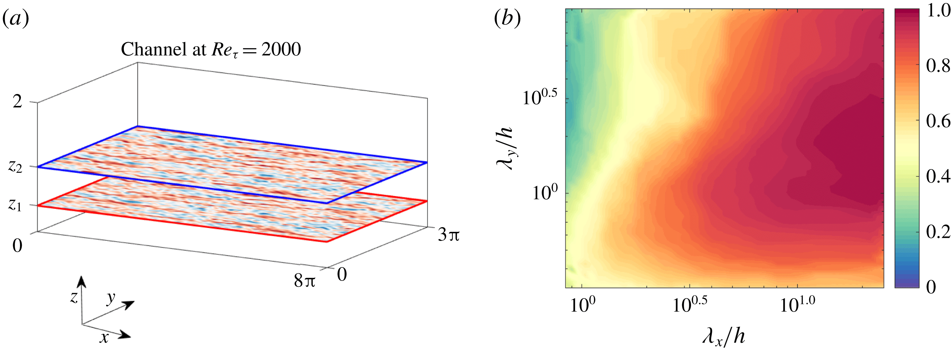
The denominator in (4.1) consists of two individual 2-D energy spectra at the wall heights $z_{1}$ and $z_{2}$ , while the numerator is the absolute value of the complex-valued cross-spectrum between the two wall heights. By definition, $0\leqslant \unicode[STIX]{x1D6FE}^{2}\leqslant 1$ , where $\unicode[STIX]{x1D6FE}^{2}=1$ indicates perfect coherence and $\unicode[STIX]{x1D6FE}^{2}=0$ indicates no coherence. Before using (4.1) to analyse the linear models, we first plot in figure 1(b) an example of the LCS using the DNS data described in § 3. Also shown in figure 1(a) is a schematic of the geometry for which the calculations are performed. We are interested in studying the coherent large-scale structures in the logarithmic layer of the flow. Hence, $z_{2}^{+}\approx 300$ ( $=0.15Re_{\unicode[STIX]{x1D70F}}$ ) is kept fixed at the end of the logarithmic layer (Marusic et al. Reference Marusic, Monty, Hultmark and Smits2013), and $z_{1}$ is taken beneath it. For the example in figure 1(b) $z_{1}^{+}\approx 200$ and the 2-D LCS is plotted as a function of $\unicode[STIX]{x1D706}_{x}/h$ and $\unicode[STIX]{x1D706}_{y}/h$ . We observe that the larger scales are more coherent than the smaller scales.

Figure 1.

(a) The geometry of the turbulent channel flow. (b) The LCS plotted for $z_{1}$ and $z_{2}$ as depicted in (a), with $z_{2}^{+}\approx 300$ ( $=0.15Re_{\unicode[STIX]{x1D70F}}$ ) kept at the end of the logarithmic layer and $z_{1}^{+}\approx 200$ .

As well as plotting the LCS for the DNS data, we can also compute it for the linear models (2.2) and (2.3). In this case, rather than using velocity signals directly, the statistically converged velocity correlations required for (4.1) are obtained by solving the Lyapunov equation (2.5). To obtain the solution, (2.2) and (2.3) are discretized in the wall-normal direction using $N_{z}=203$ Chebyshev points (see § 2). 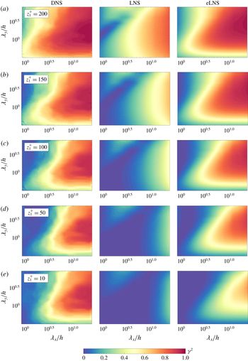The solution to (2.5) gives the velocity correlations $|\langle \hat{\boldsymbol{u}}(z_{1};k_{x},k_{y})\hat{\boldsymbol{u}}^{\ast }(z_{2};k_{x},k_{y})\rangle |$ for any combination of wall heights $z_{1}$ and $z_{2}$ , and therefore provides the correlations required for (4.1). Figure 2 shows the LCS computed for DNS, LNS and eLNS for five different values of $z_{1}$ .

Let us first consider the LCS from DNS. We start with the example shown in figure 1, which is shown again in figure 2(a). Here the first wall height, $z_{1}^{+}\approx 200$ , is relatively close to the second wall height, $z_{2}^{+}\approx 300$ , which remains fixed throughout. Moving down the rows in figure 2 (from a to e) corresponds to moving the first wall height $z_{1}$ closer to the wall and further away from $z_{2}$ . For every pair of wall heights we see that the larger scales are more coherent than the smaller scales. Interestingly, the coherence of the largest scales remains high even when $z_{1}$ is moved very close to the wall (figure 2 e). From this we can infer the existence of structures that are attached to the wall and that extend to the end of the logarithmic layer, consistent with the observations from the 1-D LCS in Baars et al. (Reference Baars, Hutchins and Marusic2017).

Now consider the LCS computed from LNS. From figure 2(a) it can be seen that, like in DNS, the large scales are more coherent than the smaller scales when $z_{1}$ and $z_{2}$ are close to each other. However, the contours from LNS in figure 2(a) look notably different from those computed from DNS. We also see that, unlike in DNS, the coherence of the large scales quickly approaches zero as $z_{1}$ moves away from $z_{2}$ and towards the wall. This indicates that the structures modelled by LNS are localized in the wall-normal direction.

Finally, we examine the LCS computed from eLNS. Figure 2(a) shows that the large scales from this model also show a higher degree of coherence than the smaller scales. The contours from eLNS look similar to those from DNS. As $z_{1}$ moves away from $z_{2}$ (from a to d), the coherence of the large scales from eLNS remains high and the contours remain similar to DNS. However, when $z_{1}$ is moved close to the wall (figure 2 e), the correspondence with DNS is lost and the large scales from the model show diminished coherence. Hence the structures from eLNS are coherent over a wider range of wall heights, but they show lower coherence than DNS in the region close to the wall.

Figure 2.

The LCS plotted from LNS and eLNS and compared with the LCS from DNS, with $z_{2}^{+}\approx 300$ ( $=0.15Re_{\unicode[STIX]{x1D70F}}$ ), and $z_{1}^{+}$ varied beneath $z_{2}^{+}$ . The plots correspond to $z_{1}^{+}\approx$ (a) 200, (b) 150, (c) 100, (d) 50 and (e) 10.

4.2 Coherence height

In § 4.1 the coherence of the large-scale structures was studied as a function of two wall-normal locations $z_{1}$ and $z_{2}$ . The coherence of the large scales from eLNS was found to be in agreement with DNS except in the near-wall region. However, it is unclear if these results are specific to the particular choice of $z_{2}^{+}\approx 300$ considered in § 4.1. Hence, to probe into the agreement between DNS and eLNS over a range of $z_{1}$ and $z_{2}$ combinations, the concept of a coherence height, as defined in Jiménez, Del Álamo & Flores (Reference Jiménez, Del Álamo and Flores2004), is now used. Since the coherence of the large scales from LNS was found to disagree with DNS, this model is not considered here. The coherence height $C_{uu}$ is defined using $\unicode[STIX]{x1D6FE}$ (from (4.1)) as

(4.2) $$\begin{eqnarray}C_{uu}(z_{0};k_{x},k_{y})=\left(\int _{0}^{z_{0}}\int _{0}^{z_{0}}\unicode[STIX]{x1D6FE}\,\text{d}z_{1}\,\text{d}z_{2}\right)^{1/2}.\end{eqnarray}$$

Since $\unicode[STIX]{x1D6FE}$ is a dimensionless quantity, $C_{uu}$ has the dimensions of length. Coherence height gives the approximate height over which a structure is coherent. The first integral in (4.2) is equivalent to calculating $\unicode[STIX]{x1D6FE}$ while keeping one probe fixed at $z_{2}$ and varying the second probe over all $z_{1}$ , such that $0\leqslant z_{1}\leqslant z_{0}$ . This returns a ‘height’ that depends on the choices of $z_{0}$ and also $z_{2}$ . The second integral calculates this height for all positions of the second probe $z_{2}$ such that $0\leqslant z_{2}\leqslant z_{0}$ and hence returns a squared height that depends only on $z_{0}$ .

The integral in (4.2) can be calculated for different values of the integration limit $z_{0}$ . The value of $z_{0}$ sets the region of the channel being considered. For a wavenumber pair $(k_{x},k_{y})$ , $C_{uu}(z_{0},k_{x},k_{y})$ considers the coherence between all combinations of wall heights $z_{1}$ and $z_{2}$ such that $0\leqslant z_{1}\leqslant z_{0}$ and $0\leqslant z_{2}\leqslant z_{0}$ . 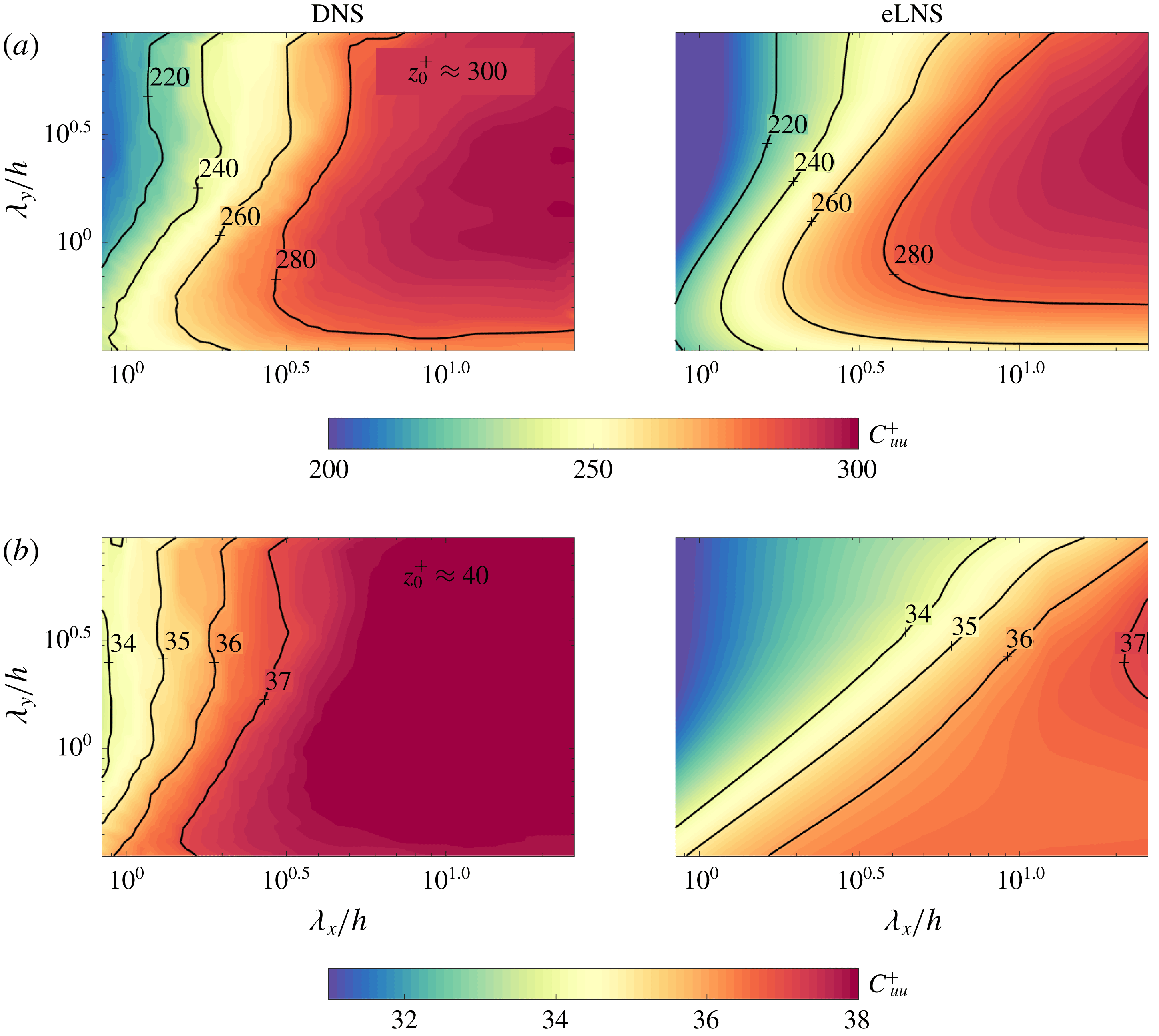Figure 3 plots the coherence height as a function of $\unicode[STIX]{x1D706}_{x}/h$ and $\unicode[STIX]{x1D706}_{y}/h$ from DNS and eLNS, for two values of $z_{0}^{+}$ : (i)  $z_{0}^{+}\approx 300$ ( $=0.15Re_{\unicode[STIX]{x1D70F}}$ ) in figure 3(a) and (ii)  $z_{0}^{+}\approx 40$ in figure 3(b).

Figure 3.

Coherence height computed from DNS and eLNS with (a)  $z_{0}^{+}\approx 300$ and (b)  $z_{0}^{+}\approx 40$ . The line contours in (a) correspond to $C_{uu}^{+}\approx (220,240,260,280)$ and in (b) to $C_{uu}^{+}\approx (34,35,36,37)$ .

First consider figure 3(a) where the coherence height is computed with $z_{0}^{+}\approx 300$ . The large-scale structures from DNS have coherence heights very close to the integration limit $z_{0}$ . This indicates that these structures extend across most of the region between the wall and $z_{0}^{+}\approx 300$ . Considering eLNS, the contours from this model in figure 3(a) approximately correspond to those from DNS, with the large scales having coherence heights close to $z_{0}$ . Hence the large-scale structures modelled by eLNS are also coherent across most of the region until the end of the logarithmic layer.

Now consider figure 3(b) where the integration limit is taken at $z_{0}^{+}\approx 40$ . We see that even in this case, the large-scale structures from DNS show coherence heights very close to $z_{0}$ , suggesting that these structures extend all the way to the wall. However, the contours from eLNS in this figure deviate in their trends from DNS, indicating that the features of the flow in the near-wall region are not captured by eLNS. Therefore, coherence of the large-scale structures are modelled reasonably well by eLNS, except in the region close to the wall. These observations are consistent with those from the LCS in § 4.1.

4.3 Scaling of the coherence spectrum

Having observed the presence of large-scale structures in eLNS that are similar to those from DNS, it is important to identify if the structures from the model are self-similar. Many authors have found evidence for the self-similar scaling of these large-scale structures and hence for Townsend’s attached eddy hypothesis in turbulent flows (e.g. Marusic Reference Marusic2001; Klewicki et al. Reference Klewicki, Fife and Wei2009; Lozano-Durán et al. Reference Lozano-Durán, Flores and Jiménez2012; Hwang Reference Hwang2015; Hellström et al. Reference Hellström, Marusic and Smits2016). The linearized Navier–Stokes equations have also been used to understand this geometric self-similarity (Del Álamo & Jiménez Reference Del Álamo and Jiménez2006; Hwang & Cossu Reference Hwang and Cossu2010b ; McKeon & Sharma Reference McKeon and Sharma2010; Moarref et al. Reference Moarref, Sharma, Tropp and McKeon2013).

Of particular relevance to this study is the coherence-based analysis carried out by Baars et al. (Reference Baars, Hutchins and Marusic2017) to demonstrate this self-similar scaling of the large-scale structures. For this purpose, Baars et al. (Reference Baars, Hutchins and Marusic2017) used the wall scaling of the experimentally obtained 1-D LCS plotted as a function of $\unicode[STIX]{x1D706}_{x}$ . Wall scaling implies that the 1-D LCS scales with $z_{2}$ , when plotted for a range of $z_{2}$ in the logarithmic layer and $z_{1}$ fixed close to the wall. Since $\unicode[STIX]{x1D706}_{x}$ represents the streamwise length of the structures, wall scaling implies the existence of self-similar structures. The streamwise lengths of the structures scale with their height, in accordance with attached eddy hypothesis.

Due to self-similarity, the spanwise dimensions of the structures should also scale with their height. The arguments in Baars et al. (Reference Baars, Hutchins and Marusic2017) can therefore be extended to two dimensions, and the contours of 2-D $\unicode[STIX]{x1D6FE}^{2}$ should scale with $z_{2}$ for a range of $z_{2}$ . For this argument, $z_{1}$ is taken close to the wall at $z_{1}^{+}\approx 40$ and $z_{2}$ is varied within the logarithmic layer, and hence $2.6\sqrt{Re_{\unicode[STIX]{x1D70F}}}\leqslant z_{2}^{+}\leqslant 0.15Re_{\unicode[STIX]{x1D70F}}$ (Klewicki et al. Reference Klewicki, Fife and Wei2009; Marusic et al. Reference Marusic, Monty, Hultmark and Smits2013). (Here $z_{1}$ is not as close to the wall as in Baars et al. (Reference Baars, Hutchins and Marusic2017), where $z_{1}^{+}\approx 4$ . This is to facilitate a comparison with eLNS where, as observed in § 4.1, the large scales show very low coherence close to the wall.)

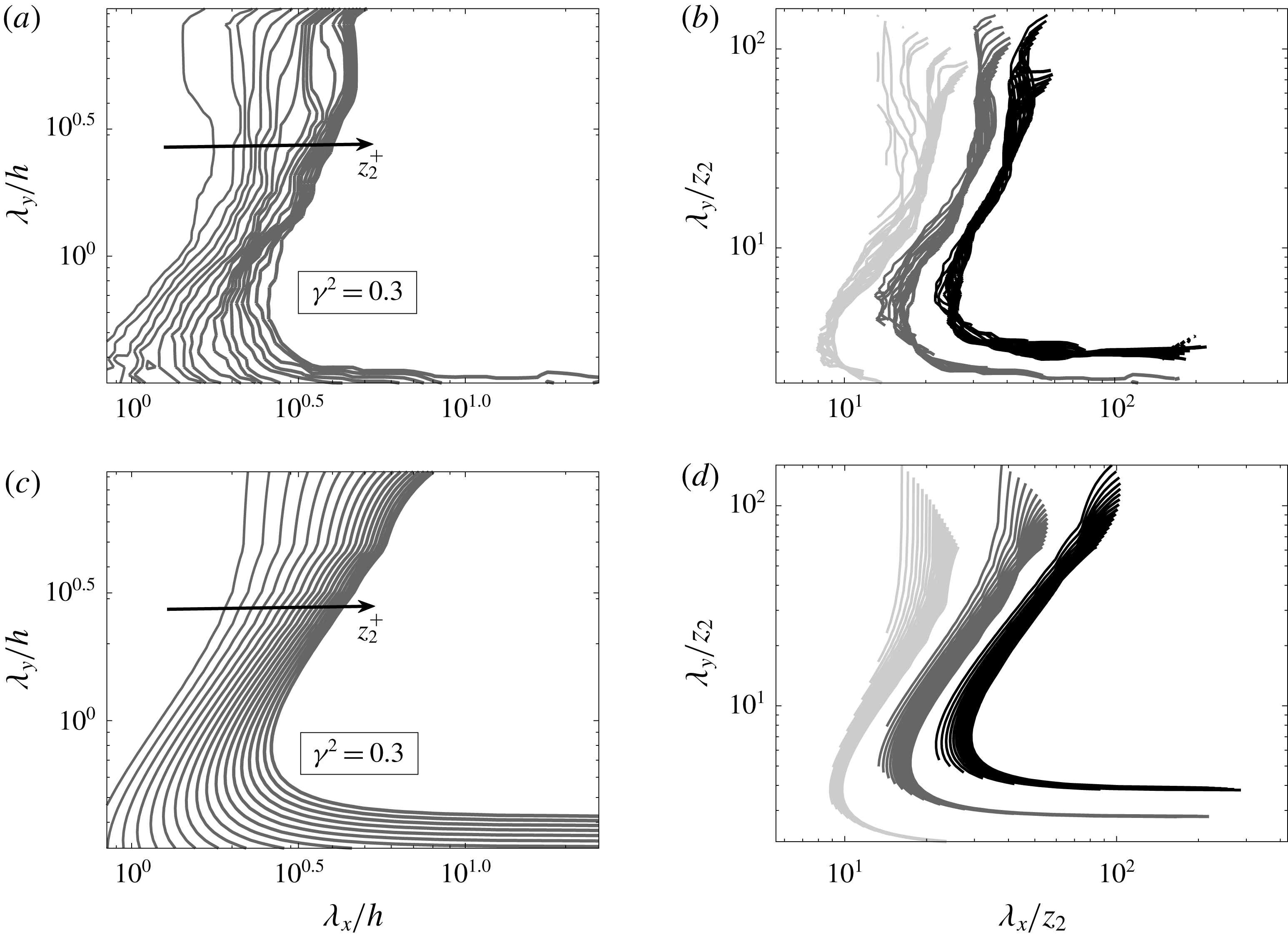
First, we verify the scaling of the 2-D $\unicode[STIX]{x1D6FE}^{2}$ using the DNS dataset. Figure 4(a) shows the contours corresponding to $\unicode[STIX]{x1D6FE}^{2}=0.3$ as a function of $(\unicode[STIX]{x1D706}_{x}/h,\unicode[STIX]{x1D706}_{y}/h)$ for a range of $z_{2}$ . Each line contour in the figure is plotted for one value of $z_{2}$ in the range considered. The contours collapse when plotted as a function of the wavelengths scaled with $z_{2}$ in figure 4(b). Figure 4(b) also shows the collapse of the contours corresponding to $\unicode[STIX]{x1D6FE}^{2}=0.1$ and $\unicode[STIX]{x1D6FE}^{2}=0.5$ . Therefore, the 2-D LCS from DNS shows wall scaling and thereby indicates the presence of self-similar structures in the flow.

Now we consider the scaling of the LCS from the linear models. The LCS from LNS does not show wall scaling. In contrast, the LCS from eLNS does scale with wall height, and therefore only the results from this model are discussed here. Figures 4(c) and 4(d) demonstrate the wall scaling of the LCS from eLNS by re-plotting figures 4(a) and 4(b), respectively, for the model. In figure 4(d) we observe the collapse of the contours when plotted as a function of $(\unicode[STIX]{x1D706}_{x}/z_{2},\unicode[STIX]{x1D706}_{y}/z_{2})$ . The contours collapse for approximately the same range of scales as in DNS. This self-similar scaling of the 2-D LCS from eLNS indicates that the model not only captures the coherence of the large-scale structures of the flow, but also captures their self-similar behaviour.

Figure 4.

The contour level corresponding to $\unicode[STIX]{x1D6FE}^{2}=0.3$ plotted for a fixed value of $z_{1}^{+}\approx 40$ and for different values of $z_{2}$ such that $2.6\sqrt{Re_{\unicode[STIX]{x1D70F}}}\leqslant z_{2}^{+}\leqslant 0.15Re_{\unicode[STIX]{x1D70F}}$ . The contours are plotted (a,b) from the DNS dataset and (c,d) from eLNS. The plots in (a,c) show the contour levels plotted as a function of $\unicode[STIX]{x1D706}_{x}/h$ and $\unicode[STIX]{x1D706}_{y}/h$ while the plots in (b,d) show the collapse of the contour levels when plotted as a function of $\unicode[STIX]{x1D706}_{x}/z_{2}$ and $\unicode[STIX]{x1D706}_{y}/z_{2}$ . Also shown in (b,d) is the collapse of the contours corresponding to $\unicode[STIX]{x1D6FE}^{2}=0.1$ and $\unicode[STIX]{x1D6FE}^{2}=0.5$ , with darker colours corresponding to higher values of $\unicode[STIX]{x1D6FE}^{2}$ .

4.4 A discussion of the coherent large-scale structures from the linear models

The 2-D LCS reveals that LNS gives rise to structures that are localized in the wall-normal direction (figure 2). This is indicative of the critical layer mechanism as described in McKeon & Sharma (Reference McKeon and Sharma2010). This critical layer mechanism gives rise to structures that are highly localized in the wall-normal direction. Considering the model eLNS, where the kinematic viscosity is augmented with an eddy viscosity profile, the large-scale structures that are modelled elongate in the wall-normal direction, and become coherent over a wider range of wall heights (figure 2). But even this model is not capable of capturing structures that show a high degree of coherence in the region close to the wall, as in DNS (figure 2 e). The computation of coherence height also shows that the coherence of the large-scale structures from eLNS agrees with DNS, except in the region near the wall (figure 3). Further, the LCS obtained from eLNS scales with wall height (figure 4 d). This shows that eLNS captures the self-similarity of the large-scale structures observed in experiments (Baars et al. Reference Baars, Hutchins and Marusic2017).

5.1 Description of SLSE

The estimation tool used here is SLSE, which was introduced in Tinney et al. (Reference Tinney, Coiffet, Delville, Hall, Jordan and Glauser2006). Before showing any results, we first review SLSE. In SLSE, a complex-valued linear transfer kernel $H_{L}(z_{1},z_{2};k_{x},k_{y})$ is defined that takes as input the Fourier coefficient of the streamwise velocity at a wavenumber pair $(k_{x},k_{y})$ and a wall height $z_{2}$ ( $\hat{u} (z_{2};k_{x},k_{y})$ ). The same quantity is estimated at a different wall height $z_{1}$ ( $\hat{u} ^{\prime }(z_{1};k_{x},k_{y})$ ), and this can be written as

(5.1) $$\begin{eqnarray}\hat{u} ^{\prime }(z_{1};k_{x},k_{y})=H_{L}(z_{1},z_{2};k_{x},k_{y})\hat{u} (z_{2};k_{x},k_{y}),\end{eqnarray}$$

where the $^{\prime }$ represents the estimated quantity.

Multiplying (5.1) with the complex conjugate of $\hat{u} (z_{2};k_{x},k_{y})$ and taking an ensemble average gives the transfer kernel $H_{L}(z_{1},z_{2};k_{x},k_{y})$ :

(5.2) $$\begin{eqnarray}H_{L}(z_{1},z_{2};k_{x},k_{y})=\frac{\langle \hat{u} (z_{1};k_{x},k_{y})\hat{u} ^{\ast }(z_{2};k_{x},k_{y})\rangle }{\langle \hat{u} (z_{2};k_{x},k_{y})\hat{u} ^{\ast }(z_{2};k_{x},k_{y})\rangle }=|H_{L}(z_{1},z_{2};k_{x},k_{y})|\text{e}^{\text{i}\unicode[STIX]{x1D713}(z_{1},z_{2};k_{x},k_{y})}.\end{eqnarray}$$

Here $\unicode[STIX]{x1D713}(z_{1},z_{2};k_{x},k_{y})$ represents the phase of the transfer kernel. The denominator in (5.2) is the 2-D energy spectrum at $z_{2}$ and the numerator is the complex-valued cross-spectrum between $z_{2}$ and $z_{1}$ . The magnitude of the transfer kernel $|H_{L}(z_{1},z_{2};k_{x},k_{y})|$ can be computed from the absolute value of the cross-spectrum and the spectrum:

(5.3) $$\begin{eqnarray}|H_{L}(z_{1},z_{2};k_{x},k_{y})|=\frac{|\langle \hat{u} (z_{1};k_{x},k_{y})\hat{u} ^{\ast }(z_{2};k_{x},k_{y})\rangle |}{|\langle \hat{u} (z_{2};k_{x},k_{y})\hat{u} ^{\ast }(z_{2};k_{x},k_{y})\rangle |}=\sqrt{\unicode[STIX]{x1D6FE}^{2}\frac{\langle |\hat{u} (z_{1};k_{x},k_{y})|^{2}\rangle }{\langle |\hat{u} (z_{2};k_{x},k_{y})|^{2}\rangle }}.\end{eqnarray}$$

The magnitude of the transfer kernel can be understood as the LCS scaled by the ratio of the 2-D energy spectra at $z_{1}$ and $z_{2}$ (Baars et al. Reference Baars, Hutchins and Marusic2016).

Only the scales that are coherent between $z_{1}$ and $z_{2}$ can be properly estimated using SLSE. In other words, if a threshold value $\unicode[STIX]{x1D6FE}_{T}^{2}$ is defined such that only the scales with $\unicode[STIX]{x1D6FE}^{2}>\unicode[STIX]{x1D6FE}_{T}^{2}$ are considered coherent, the transfer kernel $H_{L}(z_{1},z_{2};k_{x},k_{y})$ can provide correct estimates only for these coherent scales. However, $H_{L}(z_{1},z_{2};k_{x},k_{y})$ can have non-zero magnitudes at the incoherent scales with $\unicode[STIX]{x1D6FE}^{2}<\unicode[STIX]{x1D6FE}_{T}^{2}$ . Hence, using $H_{L}(z_{1},z_{2};k_{x},k_{y})$ , we will erroneously obtain estimates for these incoherent scales. To avoid this, $H_{L}(z_{1},z_{2};k_{x},k_{y})$ is set to zero for wavenumber pairs where $\unicode[STIX]{x1D6FE}^{2}<\unicode[STIX]{x1D6FE}_{T}^{2}$ , yielding a filtered transfer kernel $H_{L}(z_{1},z_{2};k_{x},k_{y})_{filt}$ (Tinney et al. Reference Tinney, Coiffet, Delville, Hall, Jordan and Glauser2006; Baars et al. Reference Baars, Hutchins and Marusic2016), which is used for estimation. Here, a threshold value of $\unicode[STIX]{x1D6FE}_{T}^{2}=0.05$ is chosen. Provided $\unicode[STIX]{x1D6FE}_{T}^{2}$ is kept sufficiently low, the exact choice of the threshold value does not have a significant effect on the results.

5.2 Estimation of the 2-D energy spectrum

Using SLSE, the 2-D energy spectrum at a wall height $z_{1}$ can be estimated using only the 2-D energy spectrum at another wall height $z_{2}$ as an input. In other words, the estimates of the 2-D energy spectrum can be obtained without directly estimating the time-resolved instantaneous velocity fields. From (5.1) we see that the estimation of the 2-D energy spectrum requires the magnitude of $H_{L}(z_{1},z_{2};k_{x},k_{y})$ and can be written as

(5.4) $$\begin{eqnarray}\unicode[STIX]{x1D719}_{uu}^{\prime }(z_{1};k_{x},k_{y})=|H_{L}(z_{1},z_{2};k_{x},k_{y})|^{2}\unicode[STIX]{x1D719}_{uu}(z_{2};k_{x},k_{y}),\end{eqnarray}$$

where $\unicode[STIX]{x1D719}_{uu}(z;k_{x},k_{y})$ represents the 2-D energy spectrum of streamwise velocity at a wall height $z$ .

5.3 Estimation using the DNS dataset

Figure 5.

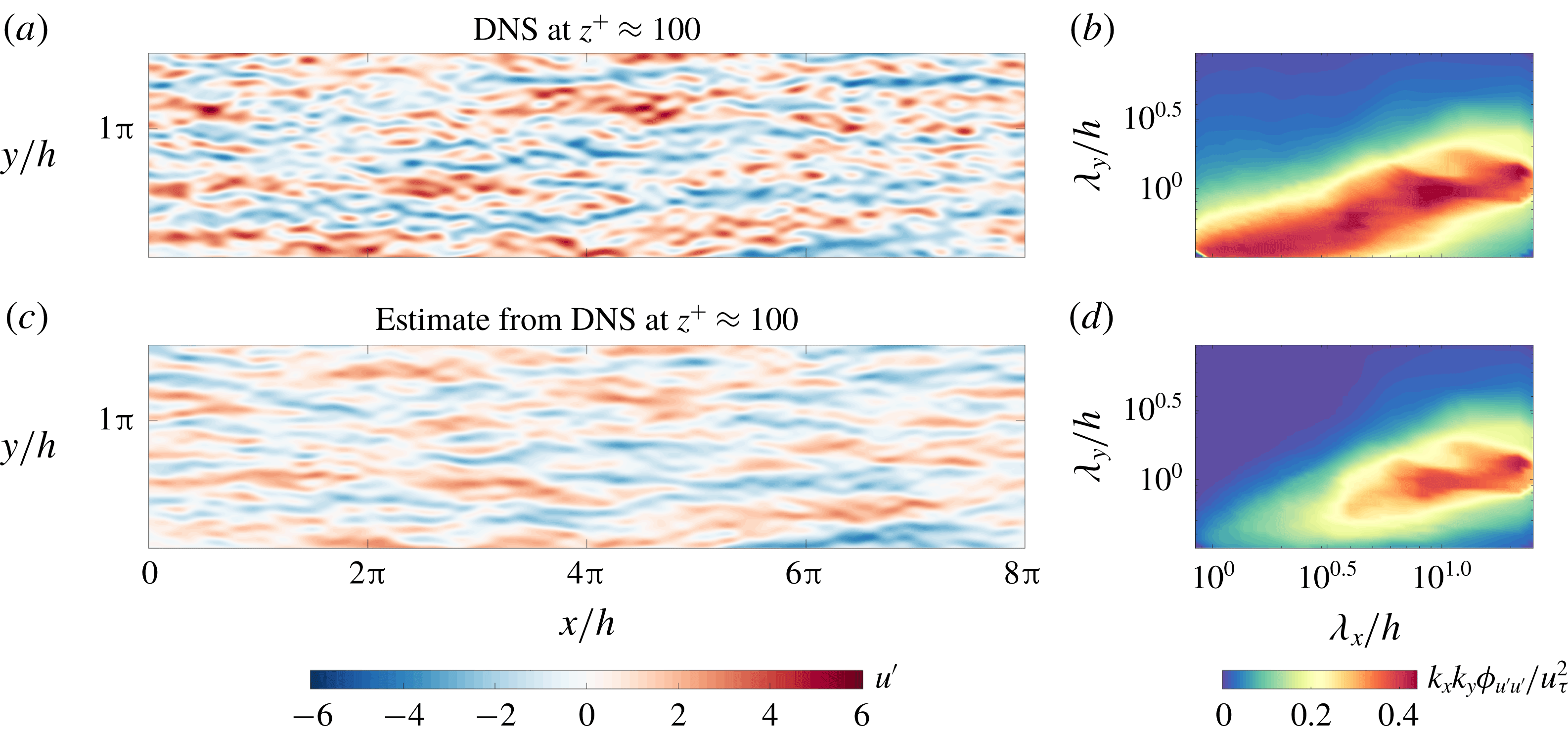
(a) The instantaneous streamwise velocity field and (b) the corresponding 2-D energy spectrum from the DNS dataset at $z_{1}^{+}\approx 100$ . (c) The instantaneous streamwise velocity field estimated at $z_{1}^{+}\approx 100$ using the DNS dataset and (d) the corresponding 2-D energy spectrum. Here $z_{2}^{+}\approx 300$ .

As an example, we consider the estimation of the velocity fluctuations and the 2-D energy spectrum at $z_{1}^{+}\approx 100$ , taking the same quantities at $z_{2}^{+}\approx 300$ as an input. Before looking at the estimation from the linear models LNS and eLNS, we require a benchmark against which the estimates from the models can later be compared. The best estimate using SLSE is that obtained by the transfer kernel $H_{L}(z_{1},z_{2};k_{x},k_{y})$ computed from DNS (Baars et al. Reference Baars, Hutchins and Marusic2016). The velocity signals from DNS are hence used to obtain the correlations required to compute $H_{L}(z_{1},z_{2};k_{x},k_{y})$ using (5.2), and the LCS computed from the same data (in § 4.1) is used to filter the transfer kernel and obtain $(H_{L}(z_{1},z_{2};k_{x},k_{y}))_{filt}$ . Using this transfer kernel, the estimated velocity field at $z_{1}$ can be obtained with the velocity field at $z_{2}$ provided as an input. This is the 2-D equivalent of the estimation done in Baars et al. (Reference Baars, Hutchins and Marusic2016) for the 1-D velocity field.

Figure 5(c) shows the estimate of the instantaneous velocity field at $z_{1}^{+}\approx 100$ obtained using the transfer kernel built from the DNS data. The corresponding 2-D energy spectrum is shown, in pre-multiplied form, in figure 5(d). According to (5.3) and (5.4), the energy spectrum of the estimated field at $z_{1}$ is simply the 2-D energy spectrum at $z_{1}$ multiplied by the LCS between $z_{1}$ and $z_{2}$ ( $\unicode[STIX]{x1D6FE}^{2}\unicode[STIX]{x1D719}_{uu}(z_{1};k_{x},k_{y})$ ). For comparison, the instantaneous velocity field and 2-D energy spectrum at $z_{1}^{+}\approx 100$ , directly obtained from the DNS dataset, are shown in figures 5(a) and 5(b) respectively. We see that only the larger scales remain in the estimated velocity field and 2-D energy spectrum at $z_{1}$ . This is because only these scales are coherent between $z_{1}$ and $z_{2}$ , as observed in § 4.1.

5.4 Estimation using the linear models

Figure 6.

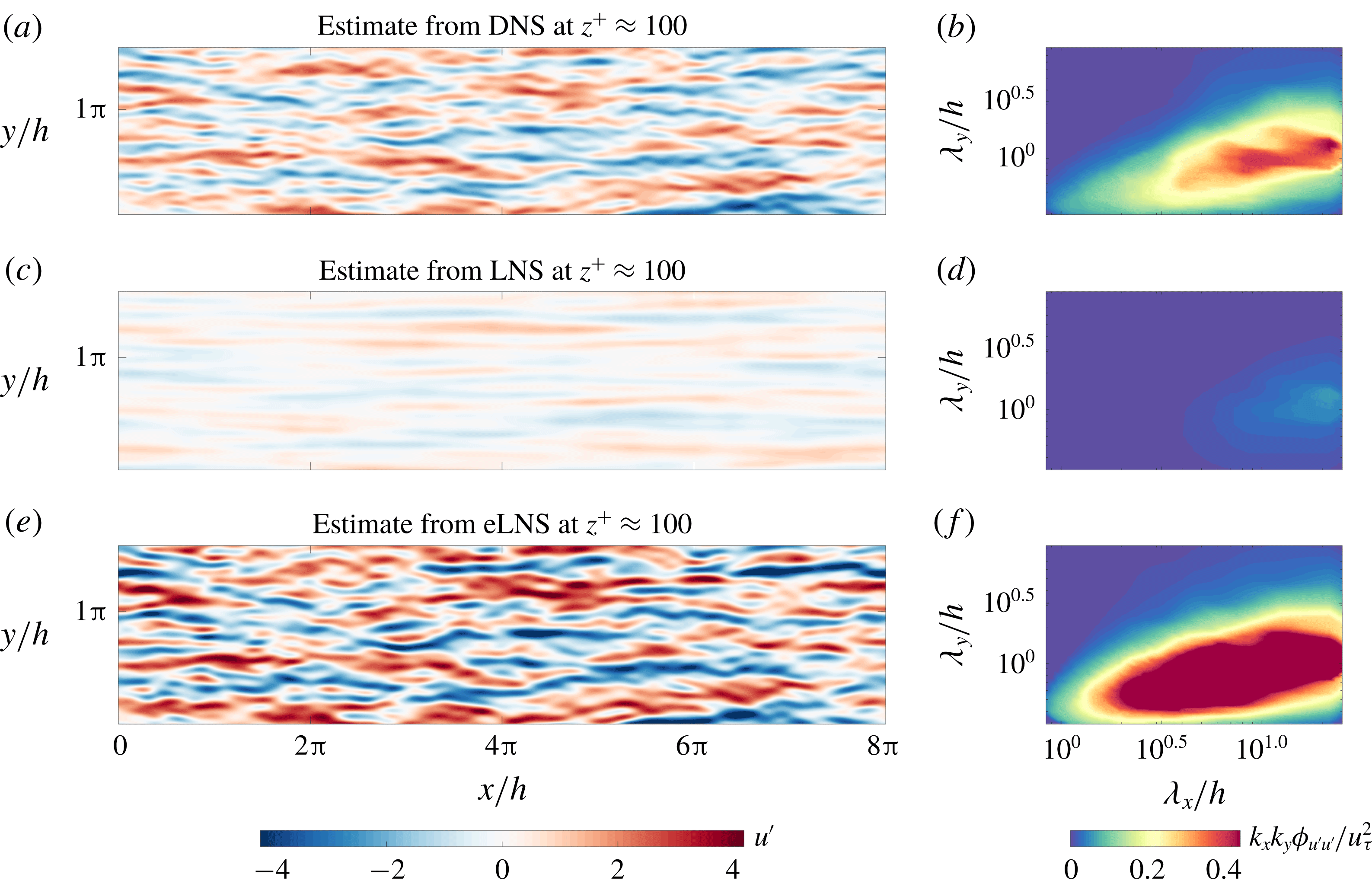
(a,c,e) The estimated instantaneous streamwise velocity field and (b,d,f) the corresponding 2-D energy spectrum obtained using (a,b) the DNS dataset, (c,d) LNS and (e,f) eLNS. The estimate is obtained at $z_{1}^{+}\approx 100$ based on a measurement at $z_{2}^{+}\approx 300$ .

Figure 7.

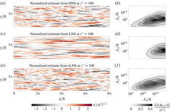
(a,c,e) The estimated instantaneous streamwise velocity field and (b,d,f) the corresponding 2-D energy spectrum obtained using (a,b) the DNS dataset, (c,d) LNS and (e,f) eLNS, normalized by $\langle {u^{\prime }}^{2}\rangle ^{1/2}$ and $\langle {u^{\prime }}^{2}\rangle$ , respectively. The estimate at $z_{1}^{+}\approx 100$ based on a measurement at $z_{2}^{+}\approx 300$ is shown. The contour lines in (b,d,f) correspond to $(k_{x}k_{y}\unicode[STIX]{x1D719}_{u^{\prime }u^{\prime }}/u_{\unicode[STIX]{x1D70F}}^{2})/\langle {u^{\prime }}^{2}\rangle =0.05,0.1$ and 0.15.

The linear models can be used in conjunction with SLSE to estimate the instantaneous velocity field and the 2-D energy spectrum. The statistically converged velocity correlations from LNS and eLNS are required to compute $H_{L}(z_{1},z_{2};k_{x},k_{y})$ for each model. These are obtained by solving the Lyapunov equation (2.5). Thereafter, the LCS computed from the models in § 4.1 is used to obtain $H_{L}(z_{1},z_{2};k_{x},k_{y})_{filt}$ . This $H_{L}(z_{1},z_{2};k_{x},k_{y})_{filt}$ computed from the models is given as an input the velocity field or the 2-D energy spectrum (from DNS) at a measurement location of $z_{2}$ . The estimated velocity field or 2-D energy spectrum at $z_{1}$ is then obtained.

Figures 6(c) and 6(e) show the estimates of the instantaneous streamwise velocity field obtained at $z_{1}^{+}\approx 100$ using a measurement at $z_{2}^{+}\approx 300$ , from LNS and eLNS, respectively. From these estimated velocity fields we see that the magnitude of the velocity fluctuations is not obtained correctly by either model. This is also reflected in the estimated 2-D energy spectra in figure 6(d,f) where, for the combination of $z_{1}$ and $z_{2}$ considered, LNS underestimates the energy of the large scales while eLNS overestimates it. We observed in § 4.1 that the large-scale structures modelled by LNS are coherent only over a narrow range of wall heights. This observation explains the underestimation of energy by this model. On the other hand, eLNS overestimates the energy even though it better models the LCS, and hence the coherence of the large-scale structures. This is because the model does not correctly obtain the magnitude of the ratio of the spectra at $z_{1}$ and $z_{2}$ that is used in (5.3).

From figure 6(e) we see that, except for the actual magnitudes, the large-scale flow features modelled by eLNS are similar to DNS. Qualitatively, we see that eLNS captures the distribution of the large-scale structures reasonably well, and therefore also approximately obtains the phase of these structures. To clarify this argument further, we normalize the estimated streamwise velocity and the energy spectra by $\langle {u^{\prime }}^{2}\rangle ^{1/2}$ and $\langle {u^{\prime }}^{2}\rangle$ , respectively. The normalization factor is computed separately for DNS, LNS and eLNS by integrating the estimated energy spectra. Figure 7 shows the normalized estimates corresponding to the estimates from DNS, LNS and eLNS in figure 6.

Considering the estimate from LNS in comparison to DNS, we see from figure 7(c) that the model estimates only the very large scales, and only these scales remain energetic in the estimated 2-D energy spectrum shown in figure 7(d). The estimate from LNS hence does not agree with those obtained from DNS. However, figure 7(e) shows that with the addition of an eddy viscosity profile, the distribution and phase of the large-scale structures are represented well by the linear model. From the estimated energy spectrum in figure 7(f) we see that the relative distribution of energy among the large-scale structures, i.e. the shape of the pre-multiplied energy spectrum, is captured reasonably well by the model.

5.5 Varying the estimation location

So far only one estimation location of $z_{1}^{+}\approx 100$ has been considered. To investigate the quality of estimation over a range of wall-normal locations, we now consider multiple estimation locations in the inner region of the flow at $10<z_{1}^{+}<200$ , as shown in figure 8. In this figure the energy spectra are normalized by the variance, as previously shown in figure 7.

Figure 8.

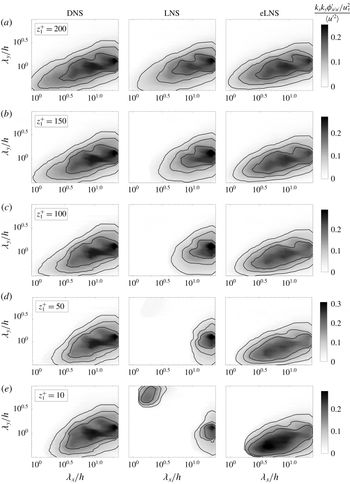
The estimates (in pre-multiplied form) of the 2-D energy spectrum normalized by $\langle {u^{\prime }}^{2}\rangle$ , from DNS, LNS and eLNS, at $z_{1}^{+}\approx$ (a) 200, (b) 150, (c) 100, (d) 50 and (e) 10, with $z_{2}^{+}\approx 300$ . The contour lines correspond to $(k_{x}k_{y}\unicode[STIX]{x1D719}_{u^{\prime }u^{\prime }}/u_{\unicode[STIX]{x1D70F}}^{2})/\langle {u^{\prime }}^{2}\rangle =0.05,0.1$ and 0.15. The regions where the estimate is zero (white) indicate scales that are incoherent and hence not estimated by the models.

We first consider the estimates obtained using LNS. As $z_{1}$ moves away from $z_{2}$ , the scales for which a non-zero estimate is obtained diminish rapidly. An explanation for this can be obtained from the trends of the LCS plotted using LNS in § 4.1, which showed that the coherence of the large scales quickly drops as $z_{1}$ moves away from $z_{2}$ . In consequence, LNS does not estimate the shape of the 2-D energy spectrum. (It should be noted that the energies estimated by LNS in figure 8(e) are very small due to the low values of coherence, and appear significant only due to the normalization.)

Now we look at the estimates obtained using eLNS. From figure 8 we see that this model provides a non-zero estimate for a wider range of $z_{1}$ . This is consistent with the conclusion made using the LCS in § 4.1 that the large-scale structures from eLNS are coherent over large wall-normal distances. Interestingly, for a range of $z_{1}$ , the shape of the 2-D pre-multiplied energy spectrum is approximately estimated by eLNS. In other words, the model captures the relative distribution of energy among the large scales reasonably well when compared with DNS. The correspondence with DNS deteriorates as $z_{1}$ moves close to the wall. This is the region where the coherence from the model was observed to be too low in comparison to DNS in § 4.1. Hence, though eLNS cannot estimate the magnitude of the 2-D energy spectrum, it can provide a reasonable estimate for the shape of the energy spectrum if $z_{1}$ is away from the wall.