1 Introduction
Large-eddy simulation (LES) is an approach that has been considered in numerical simulations of stratified turbulence (Kaltenback, Gerz & Schumann Reference Kaltenback, Gerz and Schumann1994; Armenio & Sarkar Reference Armenio and Sarkar2002; Remmler & Hickel Reference Remmler and Hickel2012; Khani & Waite Reference Khani and Waite2014, Reference Khani and Waite2015; Schaefer-Rolffs Reference Schaefer-Rolffs2016). The main goal of LES is to decrease the computational costs of direct numerical simulation (DNS), which seems to be an unnecessarily expensive numerical method because most of the computational resources are dedicated to resolving the non-energetic and viscous-affected eddies around the Kolmogorov scale
 $L_{d}$
(see e.g. Pope Reference Pope2000). In LES, we aim to directly resolve just the large energy-containing eddies, and parameterize the effects of the smaller-scale motions on resolved large eddies using the subgrid-scale (SGS) models. It has been known that, unlike isotropic turbulence, grid spacing (i.e. the smallest resolved scale) and SGS parameterizations can significantly influence the dynamics of anisotropic turbulent flows (see for example, Porté-Agel et al.
Reference Porté-Agel, Meneveau and Parlange2000; Khani & Waite Reference Khani and Waite2014, Reference Khani and Waite2015, for LES studies in atmospheric boundary layer and stratified turbulence). Khani & Waite (Reference Khani and Waite2014, Reference Khani and Waite2015) have shown the importance of resolving the buoyancy scale
 $L_{b}\sim u_{rms}/N$
in LES in order to capture the fundamental characteristics of stratified turbulence using isotropic SGS models. Here,
 $u_{rms}$
and
 $N$
are the root-mean-square (r.m.s.) velocity and buoyancy frequency, respectively (see below for the explicit definition of
 $u_{rms}$
). Also, they have shown that LES will fail if the buoyancy scale is not explicitly resolved (Khani & Waite Reference Khani and Waite2014, Reference Khani and Waite2015).
Mixing efficiency is defined as the ratio of the buoyancy flux to the mean flow turbulence production. The vertical mixing is a key parameter for researchers in the atmospheric sciences and physical oceanography. For example, it has been shown that eddy mixing has an important influence on breaking gravity waves and vertical transport of heat and tracers in geophysical turbulence (see e.g. Lilly et al.
Reference Lilly, Waco and Adelfang1974; Weinstock Reference Weinstock1978; Osborn Reference Osborn1980). Mixing efficiency has been studied numerically in stratified turbulence and shear layers (e.g. Caulfield & Peltier Reference Caulfield and Peltier2000; Shih et al.
Reference Shih, Koseff, Ivey and Ferziger2005; Salehipour & Peltier Reference Salehipour and Peltier2015; Maffioli et al.
Reference Maffioli, Brethouwer and Lindborg2016), in which turbulent diffusivity, the mixing coefficient and flux Richardson number
 $Ri_{f}$
, are modelled or estimated using DNS data. Using high resolution DNS results, Maffioli et al. (Reference Maffioli, Brethouwer and Lindborg2016) have argued that the mixing efficiency approaches a constant value when the Froude number is small. This finding is in line with DNS study of Venayagamoorthy & Stretch (Reference Venayagamoorthy and Stretch2010), where they have proposed that the mixing efficiency becomes constant when the gradient Richardson number
 $Ri$
is large. On the other hand, Shih et al. (Reference Shih, Koseff, Ivey and Ferziger2005) have shown that in weakly stratified turbulence, the mixing efficiency depends on the buoyancy Reynolds number
 $Re_{b}$
when the Froude number is
 ${\gtrsim}1$
. As a result, there is a controversy on the parameters that the mixing efficiency depends on, in the DNS approach.
The ability of LES to reproduce the correct mixing efficiency is a promising approach and active research avenue in numerical simulations of stratified turbulence, where in LES, the eddy viscosity and diffusivity are parameterized in terms of resolved variables using SGS models. For example, Armenio & Sarkar (Reference Armenio and Sarkar2002) have investigated the influences of flux Richardson number and mixing efficiency in LES of stratified channel flow. They have shown that increased stratification reduces the vertical buoyancy exchanges and turbulence levels, leading to a decrease in mixing efficiency. In this paper, we shall study mixing efficiency in LES of forced stratified turbulence, where three different SGS parameterizations are considered: the Smagorinsky (Reference Smagorinsky1963), Kraichnan (Reference Kraichnan1976) and dynamic Smagorinsky (Germano et al.
Reference Germano, Piomelli, Moin and Cabot1991) models. We compare LES results with those from DNS and hyperviscosity simulations. First, we intend to present a mathematical framework to define SGS mixing efficiency in LES. Also, we intend to estimate mixing efficiency using resolved variables by performing a scale analysis on the corresponding equations in LES. In particular, we are interested in studying the effects of capturing (or not) the buoyancy scale
 $L_{b}$
and the Ozmidov scale
 $L_{o}$
on mixing efficiency in LES of stratified turbulence. In addition, we aim to assess the performance of different SGS models in capturing the correct mixing efficiency by comparing to DNS results. The review of the literature on stratified turbulence and mixing efficiency, along with mathematical formulations, are given in § 2. Section 3 shows the simulation set-up and methodology. Results and discussion are represented in § 4, and the conclusion is given in § 5.
2 Background
At sufficiently small scales in the atmosphere and ocean where the Rossby number is large (i.e. horizontal scales below
 $\mathit{O}(100)$
km in the atmosphere and
 $\mathit{O}(1)$
km in the ocean), fluid motions are strongly affected by the stable stratification, but only weakly affected by the Earth’s rotation (Nastrom & Gage Reference Nastrom and Gage1985; Riley & Lelong Reference Riley and M.-P2000; Lindborg & Cho Reference Lindborg and Cho2001; Riley & Lindborg Reference Riley and Lindborg2008; Waite Reference Waite, von Larcher and Williams2014). In this range of scales, turbulent vortices are elongated horizontally and squeezed vertically (so-called pancake-like vortices in stratified turbulence, e.g. Waite & Bartello Reference Waite and Bartello2004; Lindborg Reference Lindborg2006; Brethouwer et al.
Reference Brethouwer, Billant, Lindborg and Chomaz2007). Therefore, we might use different length scales in the horizontal and vertical directions in stratified turbulence, as are
 ${\mathcal{L}}_{h}\sim u_{rms}^{3}/\unicode[STIX]{x1D716}$
and
 ${\mathcal{L}}_{v}\sim u_{rms}/N$
(e.g. Lindborg Reference Lindborg2006; Khani & Waite Reference Khani and Waite2013), where
 $\unicode[STIX]{x1D716}$
is the kinetic energy dissipation rate, and
 ${\mathcal{L}}_{h}$
and
 ${\mathcal{L}}_{v}$
are the horizontal and vertical length scales, respectively.
The Navier–Stokes equations under the Boussinesq approximation for resolved variables in LES of stratified turbulence, can be written as (e.g. Khani Reference Khani2015)
 $$\begin{eqnarray}\displaystyle & \displaystyle \frac{\unicode[STIX]{x2202}\bar{\boldsymbol{u}}}{\unicode[STIX]{x2202}t}+\bar{\boldsymbol{u}}\boldsymbol{\cdot }\unicode[STIX]{x1D735}\bar{\boldsymbol{u}}=-\frac{1}{\unicode[STIX]{x1D70C}_{0}}\unicode[STIX]{x1D735}\bar{p}-\frac{g}{\unicode[STIX]{x1D70C}_{0}}\bar{\unicode[STIX]{x1D70C}}\boldsymbol{e}_{z}+\unicode[STIX]{x1D735}\boldsymbol{\cdot }\unicode[STIX]{x1D749}+\bar{\boldsymbol{f}}, & \displaystyle\end{eqnarray}$$
 $$\begin{eqnarray}\displaystyle & \displaystyle \unicode[STIX]{x1D735}\boldsymbol{\cdot }\bar{\boldsymbol{u}}=0, & \displaystyle\end{eqnarray}$$
 $$\begin{eqnarray}\displaystyle & \displaystyle \frac{\unicode[STIX]{x2202}\bar{\unicode[STIX]{x1D70C}}}{\unicode[STIX]{x2202}t}+\bar{\boldsymbol{u}}\boldsymbol{\cdot }\unicode[STIX]{x1D735}\bar{\unicode[STIX]{x1D70C}}+\bar{w}\frac{\text{d}\unicode[STIX]{x1D6F7}}{\text{d}z}=\unicode[STIX]{x1D735}\boldsymbol{\cdot }\boldsymbol{h}, & \displaystyle\end{eqnarray}$$
where
 $\bar{\boldsymbol{u}}=(\bar{u},\bar{v},\bar{w})$
is the resolved velocity vector,
 $\bar{\unicode[STIX]{x1D70C}}$
and
 $\bar{p}$
are the resolved density and pressure perturbations, respectively, and
 $\bar{\boldsymbol{f}}$
is the forcing term; the molecular viscosity
 $\unicode[STIX]{x1D708}$
and diffusivity
 $\unicode[STIX]{x1D705}$
are negligible in our LES work. It is assumed that the background density field
 $\unicode[STIX]{x1D6F7}$
varies linearly with the vertical displacement
 $z$
(i.e.
 $\unicode[STIX]{x1D6F7}=-\unicode[STIX]{x1D70C}_{0}N^{2}z/g$
);
 $g$
and
 $\unicode[STIX]{x1D70C}_{0}$
are gravity and reference density, respectively; and
 $\boldsymbol{e}_{z}$
is the unique vector in the vertical direction. Note that the unresolved stress tensor
 $\unicode[STIX]{x1D749}$
and density flux
 $\boldsymbol{h}$
are unknown and require modelling using SGS parameterizations. The transport equations for the kinetic and potential energy can be obtained by multiplying
 $\bar{\boldsymbol{u}}$
and
 $\unicode[STIX]{x1D6FD}^{2}\bar{\unicode[STIX]{x1D70C}}$
, where
 $\unicode[STIX]{x1D6FD}=g/(\unicode[STIX]{x1D70C}_{0}N)$
, to equations (2.1) and (2.3), respectively, as follows
 $$\begin{eqnarray}\displaystyle & \displaystyle \frac{\unicode[STIX]{x2202}E}{\unicode[STIX]{x2202}t}+\bar{u}_{j}\frac{\unicode[STIX]{x2202}E}{\unicode[STIX]{x2202}x_{j}}=\frac{\unicode[STIX]{x2202}}{\unicode[STIX]{x2202}x_{j}}\left(-\frac{1}{\unicode[STIX]{x1D70C}_{0}}\bar{p}\bar{u}_{j}+\bar{u}_{j}\unicode[STIX]{x1D70F}_{ij}\right)-\frac{g}{\unicode[STIX]{x1D70C}_{0}}\bar{\unicode[STIX]{x1D70C}}\bar{w}-\unicode[STIX]{x1D70F}_{ij}\bar{\unicode[STIX]{x1D634}}_{ij}+\bar{f}_{j}\bar{u}_{j}, & \displaystyle\end{eqnarray}$$
 $$\begin{eqnarray}\displaystyle & \displaystyle \frac{\unicode[STIX]{x2202}}{\unicode[STIX]{x2202}t}({\mathcal{P}})+\bar{u}_{j}\frac{\unicode[STIX]{x2202}}{\unicode[STIX]{x2202}x_{j}}({\mathcal{P}})-\frac{g}{\unicode[STIX]{x1D70C}_{0}}\bar{\unicode[STIX]{x1D70C}}\bar{w}=\frac{\unicode[STIX]{x2202}}{\unicode[STIX]{x2202}x_{j}}(\unicode[STIX]{x1D6FD}^{2}h_{j}\bar{\unicode[STIX]{x1D70C}})-\unicode[STIX]{x1D6FD}^{2}h_{j}\frac{\unicode[STIX]{x2202}\bar{\unicode[STIX]{x1D70C}}}{\unicode[STIX]{x2202}x_{j}}, & \displaystyle\end{eqnarray}$$
where the kinetic energy
 $E=(1/2)\bar{u}_{i}\bar{u}_{i}$
, potential energy
 ${\mathcal{P}}=(\unicode[STIX]{x1D6FD}^{2}/2)\bar{\unicode[STIX]{x1D70C}}\bar{\unicode[STIX]{x1D70C}}$
and rate-of-strain tensor
 $\bar{\unicode[STIX]{x1D634}}_{ij}=(1/2)(\unicode[STIX]{x2202}\bar{u}_{i}/\unicode[STIX]{x2202}x_{j}+\unicode[STIX]{x2202}\bar{u}_{j}/\unicode[STIX]{x2202}x_{i})$
. We can follow a similar procedure to obtain the transport equations for the kinetic and potential energy in wavenumber (Fourier) space if we write the equations of motions (2.1)–(2.3) in wavenumber space (see e.g. Khani & Waite Reference Khani and Waite2014; Khani Reference Khani2015, for more information).
Osborn (Reference Osborn1980) has proposed an equation for mixing efficiency based on the mixing coefficient
 $\unicode[STIX]{x1D6E4}=B/\unicode[STIX]{x1D716}$
, given as
 $\unicode[STIX]{x1D6FE}_{r}=B/(B+\unicode[STIX]{x1D716})$
, where
 $B=g\langle \bar{\unicode[STIX]{x1D70C}}\bar{w}\rangle /\unicode[STIX]{x1D70C}_{0}$
is the buoyancy flux (angle bracket denotes averaging), and
 $\unicode[STIX]{x1D6FE}_{r}$
is also called the flux Richardson number
 $Ri_{f}$
. By assuming a critical mixing coefficient
 $\unicode[STIX]{x1D6E4}_{c}=0.22$
, we can get
 $\unicode[STIX]{x1D6FE}_{r}=0.18$
, a value which Osborn (Reference Osborn1980) obtained using ocean measurements. Similar definition also used lately by Shih et al. (Reference Shih, Koseff, Ivey and Ferziger2005) in DNS of sheared stratified turbulence, where they concluded that mixing efficiency depends on the buoyancy Reynolds number
 $Re_{b}$
. They have shown that the flux Richardson number
 $Ri_{f}$
is small when
 $Re_{b}\ll 1$
, it increases to an approximately constant value
 $Ri_{f}\approx 0.2$
when
 $7<Re_{b}<100$
, and
 $Ri_{f}$
decreases as
 $Re_{b}$
gets larger (Shih et al.
Reference Shih, Koseff, Ivey and Ferziger2005). Beyond this classical definition, Caulfield & Peltier (Reference Caulfield and Peltier2000) has proposed an equation for irreversible mixing efficiency based on the kinetic and potential energy dissipation rates, as follows
 $$\begin{eqnarray}\displaystyle \unicode[STIX]{x1D6FE}_{i}=\frac{\unicode[STIX]{x1D716}_{p}}{\unicode[STIX]{x1D716}+\unicode[STIX]{x1D716}_{p}}, & & \displaystyle\end{eqnarray}$$
where
 $\unicode[STIX]{x1D716}$
and
 $\unicode[STIX]{x1D716}_{p}$
are the (molecular) kinetic and potential dissipation rates, respectively. This latter definition is more desirable in the study of turbulent mixing because, unlike the former one, equation (2.6) does not consider the reversible part of mixing that is included in buoyancy flux and the flux Richardson number
 $Ri_{f}$
. This new definition has also recently been used in DNS studies of stratified turbulence (Venayagamoorthy & Stretch Reference Venayagamoorthy and Stretch2010; Salehipour & Peltier Reference Salehipour and Peltier2015; Maffioli et al.
Reference Maffioli, Brethouwer and Lindborg2016). For example, Maffioli et al. (Reference Maffioli, Brethouwer and Lindborg2016) have shown that
 $\unicode[STIX]{x1D6FE}_{i}$
is constant when the Froude number is small. In addition, using some experimental and observational evidences, it has been suggested that mixing efficiency could reach up to values approximately 0.4–0.5 (see e.g. Strang & Fernando Reference Strang and Fernando2001; Pardyjak et al.
Reference Pardyjak, Monti and Fernando2002; Peltier & Caulfield Reference Peltier and Caulfield2003). For example, Mashayek et al. (Reference Mashayek, Salehipour, Bouffard, Caulfield, Ferrari, Nikurashin, Pletier and Smyth2017) have shown that mixing efficiency could increase to be
 ${\approx}1/3$
in stratified regions of the bottom ocean near topographies. In this paper, we use (2.6) to calculate the irreversible mixing efficiency in LES of stratified turbulence. Also, we should emphasize that the kinetic and potential dissipation rates in LES are given by SGS parameterizations as
 $\unicode[STIX]{x1D716}=\unicode[STIX]{x1D70F}_{ij}\bar{\unicode[STIX]{x1D634}}_{ij}$
and
 $\unicode[STIX]{x1D716}_{p}=\unicode[STIX]{x1D6FD}^{2}h_{j}(\unicode[STIX]{x2202}\bar{\unicode[STIX]{x1D70C}}/\unicode[STIX]{x2202}x_{j})$
, where
 $\unicode[STIX]{x1D70F}_{ij}$
and
 $h_{j}$
are parameterized in terms of the resolved variables using SGS models. We use the notation
 $\unicode[STIX]{x1D6FE}_{i}$
for irreversible mixing efficiency in LES, DNS and hyperviscosity simulations. However, we should note that
 $\unicode[STIX]{x1D6FE}_{i}$
is indeed the ‘SGS’ mixing efficiency in the LES approach because the molecular viscosity (or hyperviscosity) is neglected. Nevertheless, on average and for stationary turbulence, SGS dissipation rates should be equal to molecular dissipation rates (see tables 1 and 2).
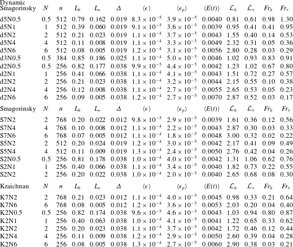
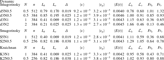
List of numerical simulations with LES.

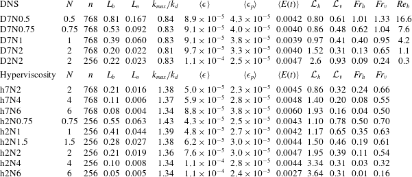
List of numerical simulations with DNS and hyperviscosity.

2.1 SGS parameterization
Common SGS parameterizations in physical space are the Smagorinsky (Reference Smagorinsky1963) and the dynamic Smagorinsky (Germano et al.
Reference Germano, Piomelli, Moin and Cabot1991) models, in which the SGS momentum stress
 $\unicode[STIX]{x1D70F}_{ij}$
and density flux
 $h_{j}$
are related to the resolved rate-of-strain tensor
 $\bar{\unicode[STIX]{x1D634}}_{ij}$
and density gradient
 $\unicode[STIX]{x2202}\bar{\unicode[STIX]{x1D70C}}/\unicode[STIX]{x2202}x_{j}$
using the eddy viscosity
 $\unicode[STIX]{x1D708}_{r}$
and diffusivity
 $\unicode[STIX]{x1D708}_{\unicode[STIX]{x1D705}}$
coefficients, respectively, given by
 $$\begin{eqnarray}\unicode[STIX]{x1D70F}_{ij}=2\unicode[STIX]{x1D708}_{r}\bar{\unicode[STIX]{x1D634}}_{ij},\quad h_{j}=\unicode[STIX]{x1D708}_{\unicode[STIX]{x1D705}}\frac{\unicode[STIX]{x2202}\bar{\unicode[STIX]{x1D70C}}}{\unicode[STIX]{x2202}x_{j}},\quad \unicode[STIX]{x1D708}_{r}=c_{s}\unicode[STIX]{x1D6E5}^{2}(2\bar{\unicode[STIX]{x1D634}}_{ij}\bar{\unicode[STIX]{x1D634}}_{ij})^{1/2},\quad \unicode[STIX]{x1D708}_{\unicode[STIX]{x1D705}}=\frac{\unicode[STIX]{x1D708}_{r}}{Pr_{t}},\end{eqnarray}$$
where
 $c_{s}$
,
 $\unicode[STIX]{x1D6E5}$
and
 $Pr_{t}$
are the Smagorinsky coefficient, grid spacing and turbulent Prandtl number, respectively. In the classical Smagorinsky (Reference Smagorinsky1963) model,
 $c_{s}=(0.17)^{2}$
, as is proposed by Lilly (Reference Lilly1967). In the dynamic Smagorinsky model, however,
 $c_{s}$
is not constant and is a time- and space-dependent variable, which is calculated dynamically by employing a coarse-filter scale
 $\tilde{\unicode[STIX]{x1D6E5}}>\unicode[STIX]{x1D6E5}$
(see e.g. Khani & Waite (Reference Khani and Waite2015), for more information about
 $c_{s}$
calculations). Similarly, we can propose a turbulent-viscosity model in wavenumber (Fourier) space, for which the spectral SGS kinetic and potential energy transfers are related to the kinetic and potential energy spectra at the cutoff wavenumber
 $k_{c}$
using spectral eddy-viscosity and diffusivity coefficients, respectively (see e.g. Kraichnan (Reference Kraichnan1976), for more information about the Kraichnan eddy-viscosity model).
3 Methodology
Idealized LES runs of forced stratified turbulence in a cubic domain of side length
 $L=2\unicode[STIX]{x03C0}$
are considered. Random AR(1) forcing is applied to the rotational part of the horizontal velocity (vortical modes). The forcing is uncorrelated in space, but correlated in time with a correlation time scale of
 $10$
time steps
 $\unicode[STIX]{x0394}t$
(as in e.g. Waite & Bartello Reference Waite and Bartello2004; Khani & Waite Reference Khani and Waite2014, Reference Khani and Waite2015). The grid spacing
 $\unicode[STIX]{x1D6E5}$
is related to the cutoff wavenumber
 $k_{c}$
, given by
 $\unicode[STIX]{x1D6E5}=\unicode[STIX]{x03C0}/k_{c}$
. The spectral transform method is considered for discretization of spatial derivatives, where the two-thirds rule (Orszag Reference Orszag1971) is employed in each direction to eliminate aliasing errors. Hence, the effective grid spacing is given by
 $\unicode[STIX]{x1D6E5}=3L/(2n)$
, where
 $n$
is the number of grid points in the
 $x$
,
 $y$
and
 $z$
directions. Also, the third-order Adams–Bashforth scheme is employed for time advancements. For comparison, we have also performed DNS and hyperviscosity simulations, in which the molecular viscosity
 $\unicode[STIX]{x1D708}$
and hyperviscosity
 $\unicode[STIX]{x1D708}_{4}$
are effective in the corresponding dissipation mechanisms (see Khani & Waite (Reference Khani and Waite2014), for more information about hyperviscosity simulations).
Simulations are initialized with random noise in low resolution (
 $n=256$
) hyperviscosity runs from time
 $t=0$
to
 $t=300$
, and then spun up to run in LES, DNS and hyperviscosity simulations from time
 $t=300$
to
 $t=450$
(the time by which simulations results have already reached a statistically stationary state; similar approaches have been followed in Khani & Waite (Reference Khani and Waite2014, Reference Khani and Waite2015)). We consider simulations resolutions from
 $n=256$
to
 $n=768$
, and the buoyancy frequency varies from
 $N=0.5$
to
 $6$
to ensure sufficiently small horizontal Froude number
 $Fr_{h}=u_{rms}/N{\mathcal{L}}_{h}$
. Results are averaged over times
 $375\leqslant t\leqslant 450$
, denoting by the angle bracket
 $\langle \cdot \rangle$
,
 $\tilde{\unicode[STIX]{x1D6E5}}=2\unicode[STIX]{x1D6E5}$
, and turbulent Prandtl number
 $Pr_{t}=1$
, which is consistent with the a priori study in DNS of stratified turbulence (see e.g. Khani & Waite Reference Khani and Waite2016). We use
 $u_{rms}=\sqrt{\langle E(t)\rangle }$
since the vertical kinetic energy is much smaller than the horizontal; and
 $L_{b}=2\unicode[STIX]{x03C0}u_{rms}/N$
. Table 1 shows a list of parameters and averaged variables in the LES runs, where the Smagorinsky, dynamic Smagorinsky and Kraichnan SGS models are considered. Also, simulation parameters and averaged variables for DNS and hyperviscosity simulations are shown in table 2, where
 $k_{max}$
and
 $k_{d}$
are the maximum and Kolmogorov wavenumbers, respectively, and the ratio
 $k_{max}/k_{d}$
shows that the resolution of the Kolmogorov scale is reasonable for all DNS and hyperviscosity simulations (i.e. in all simulations,
 $k_{max}/k_{d}>0.8$
, which is consistent with the criterion that is given by Moin & Mahesh (Reference Moin and Mahesh1998), for the resolution of
 $k_{d}$
). Here,
 $k_{d}=(\unicode[STIX]{x1D716}/\unicode[STIX]{x1D708}^{3})^{1/(6m-2)}$
, where
 $m=1$
and
 $4$
in DNS and hyperviscosity simulations, respectively. The Ozmidov scale
 $L_{o}=2\unicode[STIX]{x03C0}(\unicode[STIX]{x1D716}/N^{3})^{1/2}$
is also shown in tables 1 and 2 for LES, DNS and hyperviscosity simulations. Moreover, we perform extra LES runs with different turbulent Prandtl numbers, ranging from 0.2 to 2, to provide a complete analysis of our scaling theory for mixing efficiency (see below).
The averaged compensated horizontal wavenumber kinetic energy spectra for DNS, LES and hyperviscosity simulations: (a)
 $N=0.5$
, (b)
 $N=1$
, (c)
 $N=2$
and (d)
 $N=4$
. The horizontal axes are normalized by the buoyancy wavenumber
 $k_{b}$
, and the vertical arrows show the location of
 $k_{b}$
, where the bump (or spectral shallowness) starts. The spectra are averaged over
 $375\leqslant t\leqslant 450$
.

4 Results and discussion
4.1 Kinetic energy and SGS dissipation spectra
Figure 1 shows the time-averaged compensated horizontal wavenumber kinetic energy spectra for hyperviscosity simulations, DNS and LES, where the horizontal energy spectra are multiplied by
 $k_{h}^{5/3}\langle \unicode[STIX]{x1D716}\rangle ^{-2/3}$
. The horizontal axes are normalized by the buoyancy wavenumber
 $k_{b}$
, for which in each panel
 $k_{h}/k_{b}=1$
shows the location of the buoyancy wavenumber. Constant horizontal compensated spectra in the intermediate horizontal wavenumbers imply a
 $-5/3$
power law in the inertial subrange of the horizontal wavenumber kinetic energy spectra that is in line with the Lindborg (Reference Lindborg2006) hypothesis for stratified turbulence. For DNS, LES and hyperviscosity simulations, the
 $-5/3$
spectral slope is seen over the horizontal wavenumbers
 $0.5\lesssim k_{h}/k_{b}\lesssim 1$
when
 $N=0.5$
,
 $0.3\lesssim k_{h}/k_{b}\lesssim 0.8$
when
 $N=1$
,
 $0.2\lesssim k_{h}/k_{b}\lesssim 0.9$
when
 $N=2$
, and
 $0.1\lesssim k_{h}/k_{b}\lesssim 0.8$
when
 $N=4$
(see figure 1
a–d). Also, these constant compensated spectra are followed by a bump (or shallowness) around
 $k_{h}\sim k_{b}$
that indicates a non-local energy transfer from larger scales to the buoyancy scale
 $L_{b}=2\unicode[STIX]{x03C0}/k_{b}$
(consistent with hyperviscosity simulations, DNS and LES of Waite (Reference Waite2011), Khani & Waite (Reference Khani and Waite2013, Reference Khani and Waite2014, Reference Khani and Waite2015)). These bumps are seen around
 $k_{b}\approx 8$
,
 $16$
,
 $30$
and
 $60$
, when
 $N=0.5$
,
 $1$
,
 $2$
and
 $4$
(see the vertical arrows in figure 1, indicating the location of the buoyancy wavenumber
 $k_{b}$
). It is clear that the bump (or shallowness) occurs at
 $k_{h}/k_{b}\approx 1$
in all panels of figure 1. For example, for the dynamic Smagorinsky simulation with
 $n=512$
and
 $N=2$
, the bump (or shallowness) happens around
 $k_{h}\approx 30$
that is very close to
 $k_{b}=29.9$
(see table 1 and the dash-double-dotted red line in figure 1
c). Overall, these results show that the LES runs capture the fundamental characteristics of stratified turbulence that are in line with DNS and hyperviscosity simulations.
The horizontal and vertical SGS energy transfer spectra (eddy dissipation spectra) are shown in figure 2 (see appendix A, and also Khani & Waite (Reference Khani and Waite2014, Reference Khani and Waite2015), for calculations of the SGS eddy dissipation spectra). Interestingly, eddy dissipation spectra peak at large horizontal and small vertical scales, consistent with anisotropic dissipation in stratified turbulence (in line with effective eddy-viscosity results of Khani & Waite (Reference Khani and Waite2013), Remmler & Hickel (Reference Remmler and Hickel2014), Khani & Waite (Reference Khani and Waite2016)). The horizontal wavenumber eddy dissipation spectrum for the Kraichnan LES with
 $n=768$
and
 $N=2$
has a cusp at
 $k_{h}\approx k_{c}$
because the Kraichnan eddy-viscosity model increases near
 $k_{c}$
(see e.g. Kraichnan Reference Kraichnan1976; Métais & Lesieur Reference Métais and Lesieur1992; Khani & Waite Reference Khani and Waite2013). Increased stratification or decreased resolution increases the eddy dissipation by squeezing the buoyancy-scale thickness (vertical layer thickness) towards the dissipation scale or by increasing the dissipation scale (as seen in hyperviscosity simulations and DNS of Waite & Bartello (Reference Waite and Bartello2004), Bartello & Tobias (Reference Bartello and Tobias2013)). In addition, this anisotropic picture of eddy dissipation spectra is in agreement with the effective eddy dissipation spectra when a test-filter scale
 $\unicode[STIX]{x1D6E5}_{test}=\unicode[STIX]{x03C0}/k_{c}$
is employed around the buoyancy scale
 $L_{b}$
in DNS results (see below in figure 8).
The (a) horizontal and (b) vertical wavenumber SGS eddy dissipation spectra for LES. These spectra are calculated at
 $t=450$
, and are multiplied by wavenumber to preserve area on the log-linear axes.

4.2 Length scales
We can calculate the vertical and horizontal length scales using the corresponding averaged vertical and horizontal energy spectra in DNS, LES and hyperviscosity simulations of stratified turbulence as follows,
 $$\begin{eqnarray}{\mathcal{L}}_{v}=\frac{2\unicode[STIX]{x03C0}\displaystyle \int _{0}^{\infty }\langle E(k_{v})\rangle \,\text{d}k_{v}}{\displaystyle \int _{0}^{\infty }k_{v}\langle E(k_{v})\rangle \,\text{d}k_{v}},\quad {\mathcal{L}}_{h}=\frac{2\unicode[STIX]{x03C0}\displaystyle \int _{0}^{\infty }\langle E(k_{h})\rangle \,\text{d}k_{h}}{\displaystyle \int _{0}^{\infty }k_{h}\langle E(k_{h})\rangle \,\text{d}k_{h}},\end{eqnarray}$$
where
 $\langle E\rangle$
,
 $k_{h}$
and
 $k_{v}$
are the averaged directional resolved energy spectrum, and the horizontal and vertical wavenumbers, respectively. Figure 3 shows the ratio
 ${\mathcal{L}}_{v}/L_{b}$
versus
 $L_{b}/\unicode[STIX]{x1D6E5}$
, which is an indication of how sufficiently the buoyancy scale
 $L_{b}$
is resolved in the LES of stratified turbulence. For comparison, the results from hyperviscosity simulations and DNS are also shown. Khani & Waite (Reference Khani and Waite2014, Reference Khani and Waite2015) have shown that there is a threshold on the grid spacing
 $\unicode[STIX]{x1D6E5}$
, for which LES of stratified turbulence captures the fundamental characteristics of stratified turbulence. This threshold depends on
 $L_{b}$
and varies with different SGS models:
 $L_{b}/\unicode[STIX]{x1D6E5}>4.17$
for the dynamic Smagorinsky model,
 $L_{b}/\unicode[STIX]{x1D6E5}>5.89$
for Smagorinsky model and
 $L_{b}/\unicode[STIX]{x1D6E5}>2.13$
for the Kraichnan eddy-viscosity model (see Khani & Waite (Reference Khani and Waite2014, Reference Khani and Waite2015), these thresholds are also shown with vertical dashed lines in figure 3). It is clear that the ratio
 ${\mathcal{L}}_{v}/L_{b}$
approaches to
 $1$
when
 $L_{b}$
is well resolved in the LES, or when the buoyancy Reynolds number
 $Re_{b}=\langle \unicode[STIX]{x1D716}\rangle /(\unicode[STIX]{x1D708}N^{2})$
is sufficiently large in the DNS (note that
 $\unicode[STIX]{x1D6E5}\propto L_{d}$
in DNS, so the ratio
 $L_{b}/\unicode[STIX]{x1D6E5}$
is a measure of the size of the sub-buoyancy-scale inertial range; see figure 3, and also figure 6 in below). This trend is in line with an important feature of stratified turbulence, in which the vertical length scale is scaled by the buoyancy scale
 $L_{b}$
(i.e.
 ${\mathcal{L}}_{v}\sim L_{b}$
, see e.g. Waite Reference Waite2011; Khani & Waite Reference Khani and Waite2013).
The ratio
 ${\mathcal{L}}_{v}/L_{b}$
versus
 $L_{b}/\unicode[STIX]{x1D6E5}$
for DNS, LES and hyperviscosity simulations in stratified turbulence. The dynamic Smagorinsky, regular Smagorinsky and Kraichnan SGS models are considered in the LES runs. Vertical dashed lines (from left to right for the Kraichnan, dynamic Smagorinsky and Smagorinsky parameterizations, respectively) represent the threshold on
 $L_{b}/\unicode[STIX]{x1D6E5}$
, above which LES could capture fundamental characteristics of stratified turbulence (see e.g. Khani & Waite Reference Khani and Waite2014, Reference Khani and Waite2015). In DNS runs,
 $\unicode[STIX]{x1D6E5}\propto L_{d}$
, so the ratio
 $L_{b}/\unicode[STIX]{x1D6E5}$
is a measure of the size of the sub-buoyancy-scale inertial range.

Therefore, we can simplify the equation for vertical Froude number
 $Fr_{v}=u_{rms}/(N{\mathcal{L}}_{v})$
as follows
 $$\begin{eqnarray}Fr_{v}\sim \frac{u_{rms}}{NL_{b}}\sim \frac{L_{b}}{L_{b}}\sim 1,\end{eqnarray}$$
when
 $L_{b}/\unicode[STIX]{x1D6E5}\gg 1$
in the LES of stratified turbulence. On the other hand, when
 $L_{b}/\unicode[STIX]{x1D6E5}\lesssim 1$
,
 ${\mathcal{L}}_{v}\gg L_{b}$
, and so
 $$\begin{eqnarray}Fr_{v}=\frac{u_{rms}}{N{\mathcal{L}}_{v}}\sim \frac{L_{b}}{{\mathcal{L}}_{v}}\ll 1,\end{eqnarray}$$
in the LES of stratified turbulence, as seen in figure 3 (consistent with the behaviour of viscosity-affected stratified turbulence when
 $Re_{b}\lesssim 1$
, as seen in DNS run with
 $n=256$
and
 $N=2$
; also see Brethouwer et al.
Reference Brethouwer, Billant, Lindborg and Chomaz2007). In the next section, we will show that these two different vertical Froude number regimes in (4.2) and (4.3) have a critical influence on the scale analysis of the SGS mixing efficiency in LES of stratified turbulence.
4.3 Mixing efficiency
According to equations (2.4)–(2.7a-d ), we can write the irreversible SGS mixing efficiency in LES as follows
 $$\begin{eqnarray}\unicode[STIX]{x1D6FE}_{i}=\frac{\langle (\unicode[STIX]{x1D6FD}^{2}/Pr_{t})(\unicode[STIX]{x2202}\bar{\unicode[STIX]{x1D70C}}/\unicode[STIX]{x2202}x_{j})(\unicode[STIX]{x2202}\bar{\unicode[STIX]{x1D70C}}/\unicode[STIX]{x2202}x_{j})\rangle }{\langle 2\bar{\unicode[STIX]{x1D634}}_{ij}\bar{\unicode[STIX]{x1D634}}_{ij}\rangle +\langle (\unicode[STIX]{x1D6FD}^{2}/Pr_{t})(\unicode[STIX]{x2202}\bar{\unicode[STIX]{x1D70C}}/\unicode[STIX]{x2202}x_{j})(\unicode[STIX]{x2202}\bar{\unicode[STIX]{x1D70C}}/\unicode[STIX]{x2202}x_{j})\rangle }.\end{eqnarray}$$
Next, we are interested in performing scale analysis on
 $\unicode[STIX]{x1D6FE}_{i}$
by using the scale of resolved variables in the right-hand side of equation (4.4). If we assume
 ${\mathcal{L}}_{v}\ll {\mathcal{L}}_{h}$
, which is a reasonable assumption in stratified turbulence (see table 1), we can write (following to Khani & Porté-Agel Reference Khani and Porté-Agel2017)
 $$\begin{eqnarray}\frac{g}{\unicode[STIX]{x1D70C}_{0}}\frac{\unicode[STIX]{x2202}\bar{\unicode[STIX]{x1D70C}}}{\unicode[STIX]{x2202}x_{j}}\sim N^{2},\quad \bar{\unicode[STIX]{x1D634}}_{ij}\sim \frac{u_{rms}}{{\mathcal{L}}_{v}},\end{eqnarray}$$
and so,
 $$\begin{eqnarray}\unicode[STIX]{x1D6FE}_{i}\sim \frac{N^{2}/Pr_{t}}{2(u_{rms}^{2}/{\mathcal{L}}_{v}^{2})+N^{2}/Pr_{t}}\sim \frac{1}{2Pr_{t}Fr_{v}^{2}+1}.\end{eqnarray}$$
Moreover, in the stratified turbulence regime
 $Fr_{v}\sim 1$
(as is given by (4.2), also see e.g. Billant & Chomaz Reference Billant and Chomaz2001; Waite & Bartello Reference Waite and Bartello2004; Lindborg Reference Lindborg2006; Waite Reference Waite2011; Khani & Waite Reference Khani and Waite2013; Khani Reference Khani2015), which results in
 $$\begin{eqnarray}\unicode[STIX]{x1D6FE}_{i}\sim \frac{1}{2Pr_{t}+1}.\end{eqnarray}$$
This scaling theory is supported by simulations at different turbulent Prandtl numbers
 $Pr_{t}$
, which are discussed below in § 4.6. We can write an equality relation for the scaling theory (4.7) as follows
 $$\begin{eqnarray}\unicode[STIX]{x1D6FE}_{i}=\frac{c}{2Pr_{t}+1},\end{eqnarray}$$
where
 $c$
is a proportionality constant, and we may estimate it using LES data. We have employed the least-squares method to measure
 $c$
using our LES runs, where the turbulent Prandtl number
 $Pr_{t}$
varies from
 $0.2$
to
 $2$
. It is shown that the estimated value for the coefficient
 $c$
depends on the SGS scheme and grid spacing, but is fairly close to
 $1$
(see appendix B). Therefore, we set
 $c\approx 1$
in the equality relation (4.8). Assuming
 $Pr_{t}\approx 1$
(see below in figure 9 and also in Khani & Waite Reference Khani and Waite2016), we can obtain a theoretical estimate for the irreversible SGS mixing efficiency
 $\unicode[STIX]{x1D6FE}_{i}$
in the stratified turbulence regime as follows
 $$\begin{eqnarray}\unicode[STIX]{x1D6FE}_{i}\approx {\textstyle \frac{1}{3}},\end{eqnarray}$$
which is slightly larger than the value that is observed in recent DNS studies (see e.g. Venayagamoorthy & Stretch Reference Venayagamoorthy and Stretch2010; Maffioli et al.
Reference Maffioli, Brethouwer and Lindborg2016). It is important to mention that all parameters and variables are scaled except the turbulent Prandtl number, which is approximated by
 $1$
, to obtain equation (4.9); therefore, this equation gives an estimate for the scale of the irreversible mixing efficiency
 $\unicode[STIX]{x1D6FE}_{i}$
. In the rest of this section, we will show that the LES results are in good agreement with those from DNS and hyperviscosity simulations and the scale analysis in equation (4.9).
The irreversible mixing efficiency
 $\unicode[STIX]{x1D6FE}_{i}$
versus (a) the vertical Froude number
 $Fr_{v}$
and (b) the horizontal Froude number
 $Fr_{h}$
, for DNS, LES and hyperviscosity simulations. We have considered
 $2\unicode[STIX]{x03C0}$
factors in definitions of
 $Fr_{v}$
and
 $Fr_{h}$
to remove the effects of
 $2\unicode[STIX]{x03C0}$
factors, which are used in definitions of
 ${\mathcal{L}}_{v}$
and
 ${\mathcal{L}}_{h}$
, respectively, as seen in (4.1). The violet cross sign in panel (a) shows the theoretical scale analysis of
 $\unicode[STIX]{x1D6FE}_{i}$
for LES approach as given in (4.9).

Figure 4 shows the irreversible SGS mixing efficiency
 $\unicode[STIX]{x1D6FE}_{i}$
versus the vertical Froude number
 $Fr_{v}$
in panel (a) and the horizontal Froude number
 $Fr_{h}$
in panel (b) for the dynamic Smagorinsky, regular Smagorinsky and Kraichnan SGS models. For comparison, the results from hyperviscosity simulations and DNS are also shown. Here, we have considered a
 $2\unicode[STIX]{x03C0}$
factor in definitions of
 $Fr_{v}$
and
 $Fr_{h}$
to remove the effects of the
 $2\unicode[STIX]{x03C0}$
factor in the definitions of
 ${\mathcal{L}}_{v}$
and
 ${\mathcal{L}}_{h}$
, respectively, as are given in (4.1). Interestingly, the curves for the irreversible SGS mixing efficiency in LES are fairly close to those of the irreversible mixing efficiency in DNS. The mixing efficiency
 $\unicode[STIX]{x1D6FE}_{i}$
is small when
 $Fr_{v}$
is small, and it goes to the value
 $1/3$
as
 $Fr_{v}$
increases towards
 $1$
(figure 4
a). The violet cross sign in figure 4(a) shows the theoretical value of
 $\unicode[STIX]{x1D6FE}_{i}$
(as given by (4.9)). Importantly, equation (4.9) is only valid in LES approach when
 $Fr_{v}\sim 1$
because this is the situation that
 ${\mathcal{L}}_{v}\sim L_{b}$
(see (4.2)). As
 $Fr_{v}\rightarrow 1$
, LES results approach the theoretical value
 $\unicode[STIX]{x1D6FE}_{i}\approx 1/3$
(see figure 4
a). It is interesting that DNS and the dynamic Smagorinsky LES perform similarly (see black and blue lines in figure 4). The maximum irreversible mixing efficiency
 $\unicode[STIX]{x1D6FE}_{i}$
is given by
 $0.33$
in DNS run with
 $n=768$
and
 $N=0.5$
, and it is given by
 $0.32$
(
 $0.31$
) in the dynamic Smagorinsky simulation with
 $n=512$
(
 $256$
) and
 $N=0.5$
. This behaviour shows that the dynamic Smagorinsky model performs reasonably well even at lower resolution simulations in comparison with high resolution DNS runs. The performance of the regular Smagorinsky model is less efficient in comparison with the Kraichnan model and the maximum of
 $\unicode[STIX]{x1D6FE}_{i}$
is
 $0.29$
and
 $0.32$
, respectively, in the Smagorinsky and Kraichnan simulations with
 $n=256$
and
 $N=0.5$
. As
 $Fr_{v}$
(or
 $Fr_{h}$
) decreases, the irreversible SGS mixing efficiency
 $\unicode[STIX]{x1D6FE}_{i}$
reduces (figure 4). Also, we should mention that simulations are mostly in the range of small horizontal Froude number, and
 $Fr_{h}$
increases as
 $N$
decreases (moving from the strongly stratified to weakly stratified regime, see § 4.4). The hyperviscosity simulations show slightly higher
 $\unicode[STIX]{x1D6FE}_{i}$
even at
 $Fr_{v}\approx 0.7$
(figure 4
a). This trend could be due to the effects of hyperviscosity that constrains the dissipation range to much smaller scales in comparison with regular viscosity, and so slightly decreases the averaged kinetic dissipation rates (see table 2).
We have suggested different regimes for
 $Fr_{v}$
in LES of stratified turbulence based on the resolution of the buoyancy scale
 $L_{b}$
(see (4.2) and (4.3)). Hence, it will be important to investigate if
 $\unicode[STIX]{x1D6FE}_{i}$
does depend on the resolution of
 $L_{b}$
or not. We will do a similar investigation to study the dependence of
 $\unicode[STIX]{x1D6FE}_{i}$
on the resolution of
 $L_{o}$
in the next section. Figure 5 shows
 $\unicode[STIX]{x1D6FE}_{i}$
versus
 $L_{b}/\unicode[STIX]{x1D6E5}$
for different SGS parameterizations in LES, and also for hyperviscosity simulations and DNS (vertical dashed lines in figure 5 represent the thresholds on
 $L_{b}/\unicode[STIX]{x1D6E5}$
, respectively from left to right, for the Kraichnan, dynamic Smagorinsky and Smagorinsky models). It is clear that for all SGS parameterizations, as the ratio
 $L_{b}/\unicode[STIX]{x1D6E5}$
increases, the irreversible SGS mixing efficiency
 $\unicode[STIX]{x1D6FE}_{i}$
rises and approaches the theoretical value
 $1/3$
(see (4.9) and figure 5). This trend suggests that if the buoyancy scale
 $L_{b}$
is well resolved in LES, the mixing efficiency
 $\unicode[STIX]{x1D6FE}_{i}$
is in line with the results of the theoretical scale analysis in LES of stratified turbulence, and if the threshold
 $L_{b}/\unicode[STIX]{x1D6E5}$
is violated, LES of stratified turbulence underestimates the irreversible SGS mixing efficiency
 $\unicode[STIX]{x1D6FE}_{i}$
(figure 5). This behaviour is in agreement with DNS runs, in which the irreversible mixing efficiency
 $\unicode[STIX]{x1D6FE}_{i}$
increases monotonically with
 $L_{b}/\unicode[STIX]{x1D6E5}$
(see black line in figure 5; note that
 $\unicode[STIX]{x1D6E5}\propto L_{d}$
in DNS). Figure 6 shows the irreversible mixing efficiency versus the buoyancy Reynolds number
 $Re_{b}$
in DNS runs. Clearly,
 $\unicode[STIX]{x1D6FE}_{i}$
increases respectively from
 $0.18$
to
 $0.33$
when the buoyancy Reynolds number increases from
 $Re_{b}\approx 0.3$
, where the layered stratified flows are mainly affected by viscous sublayers, to
 $Re_{b}\approx 17$
, where overturning and Kelvin–Helmholtz instabilities are ubiquitous in stratified turbulence (in line with DNS results of Shih et al.
Reference Shih, Koseff, Ivey and Ferziger2005).
The irreversible mixing efficiency
 $\unicode[STIX]{x1D6FE}_{i}$
versus the ratio
 $L_{b}/\unicode[STIX]{x1D6E5}$
for DNS, LES and hyperviscosity simulations. See the caption in figure 3 for more information about the vertical dashed lines.

The irreversible mixing efficiency
 $\unicode[STIX]{x1D6FE}_{i}$
versus the buoyancy Reynolds number
 $Re_{b}=\langle \unicode[STIX]{x1D716}\rangle /(\unicode[STIX]{x1D708}N^{2})$
for DNS runs.

Overall, depending on the resolution of the buoyancy scale
 $L_{b}$
, LES of stratified turbulence will underestimate
 $\unicode[STIX]{x1D6FE}_{i}$
if
 $L_{b}$
in not adequately resolved (similar to DNS runs with
 $Re_{b}\lesssim 1$
), or LES will correctly resemble
 $\unicode[STIX]{x1D6FE}_{i}$
if
 $L_{b}$
is well resolved, i.e.
 $L_{b}/\unicode[STIX]{x1D6E5}\gtrsim 10$
as seen in figures 3 and 5 (similar to DNS runs with
 $Re_{b}\gtrsim 10$
). In addition, the regular Smagorinsky parameterization still underestimates
 $\unicode[STIX]{x1D6FE}_{i}$
when
 $N$
is large even for the highest resolution simulations, but both the Kraichnan and dynamic Smagorinsky models represents reasonable results when
 $L_{b}$
is more likely well resolved (see figures 4 and 5). This behaviour is due to the highly dissipative nature of the regular Smagorinsky model (as is also reported in Khani & Waite (Reference Khani and Waite2014, Reference Khani and Waite2015)). These results suggest that reproducing correct mixing efficiency in the LES approach requires much better resolution of
 $L_{b}$
in comparison with, for example, reproducing correct energy spectra in LES. In the next section, we study the effects of resolving
 $L_{o}$
in mixing efficiency for LES of stratified turbulence.
4.4 Ozmidov-scale effects
In stratified turbulence, the ratio of the Ozmidov scale
 $L_{o}$
to the buoyancy scale
 $L_{b}$
can be scaled as
 $$\begin{eqnarray}\frac{L_{o}}{L_{b}}\sim Fr_{h}^{1/2},\end{eqnarray}$$
where we have used Taylor’s hypothesis
 ${\mathcal{L}}_{h}\sim u_{rms}^{3}/\unicode[STIX]{x1D716}$
. When
 $Fr_{h}\ll 1$
, which is the case in strongly stratified turbulent flows,
 $L_{o}\ll L_{b}$
(see (4.10)). Therefore, if
 $L_{o}$
is resolved (i.e.
 $L_{o}\gtrsim \unicode[STIX]{x1D6E5}$
), the resolution of
 $L_{b}$
is ensured (i.e.
 $L_{b}\gg \unicode[STIX]{x1D6E5}$
). In this situation
 ${\mathcal{L}}_{v}\sim u_{rms}/N$
(as in (4.2)), and we can scale
 $Fr_{h}$
as follows
 $$\begin{eqnarray}Fr_{h}=\frac{u_{rms}}{N{\mathcal{L}}_{h}}\sim \frac{{\mathcal{L}}_{v}}{{\mathcal{L}}_{h}},\end{eqnarray}$$
where
 ${\mathcal{L}}_{v}\ll {\mathcal{L}}_{h}$
(anisotropic motions). Using (4.10) and (4.11), we can conclude that
 $$\begin{eqnarray}\frac{L_{o}}{L_{b}}\sim \left(\frac{{\mathcal{L}}_{v}}{{\mathcal{L}}_{h}}\right)^{1/2},\end{eqnarray}$$
in the strongly stratified turbulence regime. If the turbulence regime moves from strongly stratified to weakly stratified (and so forth to the isotropic Kolmogorov turbulence),
 ${\mathcal{L}}_{v}\rightarrow {\mathcal{L}}_{h}$
(isotropic motions), and thus
 $L_{o}\rightarrow L_{b}$
(see (4.12)). As a result, weakly stratified means
 $Fr_{h}\sim \mathit{O}(1)$
, which is in agreement with (4.10).
Figure 7 shows the ratio
 ${\mathcal{L}}_{v}/L_{b}$
and
 $\unicode[STIX]{x1D6FE}_{i}$
versus
 $L_{o}/\unicode[STIX]{x1D6E5}$
in panels (a) and (b), respectively, for DNS, LES and hyperviscosity simulations. It is clear that
 ${\mathcal{L}}_{v}\approx L_{b}$
when
 $L_{o}/\unicode[STIX]{x1D6E5}\gtrsim 1$
(figure 7
a). This trend is expected because if
 $L_{o}$
is more likely resolved in LES of stratified turbulence where
 $Fr_{h}\ll 1$
, it is guaranteed that
 $L_{b}$
is well resolved (see (4.10)). In addition, the irreversible mixing efficiency
 $\unicode[STIX]{x1D6FE}_{i}$
moves towards the theoretical value
 $1/3$
if
 $L_{o}$
is resolved in LES of stratified turbulence (figure 7
b). These results show that if
 $\unicode[STIX]{x1D6E5}\lesssim L_{o}$
in LES of stratified turbulence, the mixing efficiency is correctly reproduced.
(a) The ratio
 ${\mathcal{L}}_{v}/L_{b}$
and (b) irreversible mixing efficiency
 $\unicode[STIX]{x1D6FE}_{i}$
versus the ratio
 $L_{o}/\unicode[STIX]{x1D6E5}$
for DNS, LES and hyperviscosity simulations. In DNS,
 $\unicode[STIX]{x1D6E5}\propto L_{d}$
, and therefore
 $L_{o}/\unicode[STIX]{x1D6E5}$
is a measure of
 $Re_{b}$
(i.e. large
 $L_{o}/\unicode[STIX]{x1D6E5}$
in DNS refers to stratified turbulence regime with
 $Re_{b}\gg 1$
).

Overall, these results are in line with those from figures 3 and 5. Consequently, if
 $\unicode[STIX]{x1D6E5}\lesssim L_{o}$
, irreversible mixing efficiency goes to the theoretical value
 $1/3$
(see figures 5 and 7). In addition, the fundamental characteristics of stratified turbulence, such as anisotropic features, are more likely captured because the buoyancy scale
 $L_{b}$
is well resolved (see e.g. Khani & Waite Reference Khani and Waite2014, Reference Khani and Waite2015; Khani & Porté-Agel Reference Khani and Porté-Agel2017) when
 $\unicode[STIX]{x1D6E5}\lesssim L_{o}$
.
4.5 An a priori study using DNS results
In this section, we calculate the spectra of effective SGS energy transfer (eddy dissipation) and turbulent Prandtl number by applying a test cutoff wavenumber
 $k_{c}$
, which is around the buoyancy wavenumber
 $k_{b}$
, to DNS data (see appendix A, and also Khani & Waite Reference Khani and Waite2016, for calculations of the effective eddy dissipation spectra). Figure 8 shows the horizontal and vertical wavenumber spectra for effective eddy dissipation. These plots should be compared with the SGS eddy dissipation spectra that are shown in figure 2. We consider
 $k_{c}=20$
for DNS cases with
 $N=0.5$
,
 $0.75$
and
 $1$
, and
 $k_{c}=40$
for the DNS case with
 $N=2$
(these values are around the buoyancy wavenumber
 $k_{b}=2\unicode[STIX]{x03C0}/L_{b}$
; see table 2). The effective eddy dissipation spectra also peak at large horizontal and small vertical scales (in line with the anisotropic dissipation picture, and are consistent with the corresponding SGS eddy dissipation spectra that are shown in figure 2). These trends strongly suggest that the dissipation mechanism in stratified turbulence includes anisotropic features around the buoyancy scale
 $L_{b}$
, and that is different than the dissipation mechanism in isotropic turbulence. When the test-filter wavenumber
 $k_{c}$
is fixed, increased buoyancy frequency
 $N$
results in increasing the non-local horizontal (i.e.
 $k_{h}\ll k_{c}$
) and local vertical (i.e.
 $k_{v}\sim k_{c}$
) effective eddy dissipation in simulations with
 $N=0.5$
,
 $0.75$
and
 $1$
, because the buoyancy scale
 $L_{b}$
becomes smaller than the filter width
 $\unicode[STIX]{x1D6E5}_{test}=\unicode[STIX]{x03C0}/k_{c}$
, and thus the anisotropic motions are mainly filtered (figure 8 and table 2). Overall, resolving the buoyancy scale in the LES approach is a critical threshold in order to capture the fundamental characteristics of stratified turbulence (in line with LES and DNS results of Khani & Waite Reference Khani and Waite2014, Reference Khani and Waite2015, Reference Khani and Waite2016; Khani & Porté-Agel Reference Khani and Porté-Agel2017).
The (a) horizontal and (b) vertical wavenumber effective eddy dissipation spectra in DNS runs. The spectra are calculated at
 $t=450$
, and are multiplied by wavenumber to preserve area on the log-linear axes. We employ the test cutoff wavenumber
 $k_{c}=40$
in the DNS run with
 $N=2$
, and
 $k_{c}=20$
in other DNS runs. These plots should be compared to the corresponding SGS eddy dissipation spectra that are shown in figure 2.

The spectra of effective turbulent Prandtl number are shown in figure 9. We define
 $Pr_{t}(k|k_{c})$
as the ratio of the effective eddy viscosity
 $\unicode[STIX]{x1D708}_{e}(k|k_{c})$
over the effective eddy diffusivity
 $D_{e}(k|k_{c})$
(as are given in appendix A, and also in Khani & Waite Reference Khani and Waite2016). The turbulent Prandtl number spectra show approximately constant trends when
 $k/k_{c}\gtrsim 0.2$
(consistent with the results of Khani & Waite Reference Khani and Waite2016, and this also demonstrates that the assumption of
 $Pr_{t}\approx 1$
in this current work is a reasonable approximation).
The effective turbulent Prandtl number spectra for DNS runs. The spectra are calculated at
 $t=450$
. We employ the test cutoff wavenumber
 $k_{c}=40$
in the DNS run with
 $N=2$
, and
 $k_{c}=20$
in other DNS runs. The solid and dashed magenta lines indicate values of zero and
 $1$
, respectively.

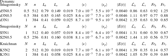
List of numerical simulations with LES when
 $Pr_{t}=0.2$
.

4.6 Turbulent Prandtl number effects
In stratified turbulence,
 $Pr_{t}\approx 1$
(as is shown in figure 9; and also see Salehipour & Peltier Reference Salehipour and Peltier2015; Khani & Waite Reference Khani and Waite2016), which leads to a scale of around
 $1/3$
for the irreversible mixing efficiency in LES of stratified turbulence (see (4.9)) that is in line with DNS results. Nevertheless, it is still very interesting to test the scaling theory (4.7) with different turbulent Prandtl numbers. We have performed extra LES runs when
 $Pr_{t}$
varies from
 $0.2$
to
 $2$
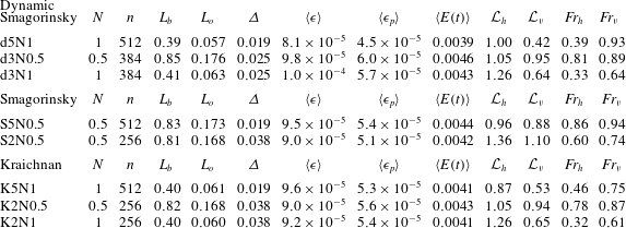
. Tables 3, 4 and 5 show simulation parameters and averaged variables for these LES runs. Using these new simulations, we can evaluate the dependency of the irreversible mixing efficiency
 $\unicode[STIX]{x1D6FE}_{i}$
on the turbulent Prandtl number
 $Pr_{t}$
as is given by scaling theory (4.7), and also we can estimate the proportionality coefficient
 $c$
in (4.8), as shown in appendix B. Figure 10 shows
 $\unicode[STIX]{x1D6FE}_{i}$
versus
 $Pr_{t}$
for the dynamic Smagorinsky, regular Smagorinsky and Kraichnan SGS models. For comparison, the scaling theory (4.7) is also shown with a black dashed line. It is clear that
 $\unicode[STIX]{x1D6FE}_{i}$
increases (decreases) when
 $Pr_{t}$
decreases (increases), and that LES results are in line with the scaling theory (figure 10). When
 $Pr_{t}\gtrsim 1$
, the scaling theory (4.7) agrees very well with the LES results, however, it slightly overestimates
 $\unicode[STIX]{x1D6FE}_{i}$
when
 $Pr_{t}<1$
. For example, the dynamic Smagorinsky model with
 $n=384$
,
 $N=1$
and
 $Pr_{t}=2$
gives
 $\unicode[STIX]{x1D6FE}_{i}=0.20$
, which equals to the scaling theory value in (4.7) when
 $Pr_{t}=2$
. Similar results are given by the Smagorinsky model with
 $n=512$
and
 $N=1$
, and the Kraichnan model with
 $n=384$
and
 $N=1$
. When
 $Pr_{t}=0.5$
, the dynamic Smagorinsky model with
 $n=384$
and
 $N=0.5$
gives
 $\unicode[STIX]{x1D6FE}_{i}=0.38$
, which is below the given value by the theoretical scale analysis curve with
 $\unicode[STIX]{x1D6FE}_{i}\approx 0.5$
. Similar trends are seen in the Smagorinsky and Kraichnan models. Also when
 $Pr_{t}=0.2$
, the dynamic Smagorinsky model with
 $n=384$
and
 $N=1$
gives
 $\unicode[STIX]{x1D6FE}_{i}=0.52$
, which is below the given estimate with scaling theory
 $\unicode[STIX]{x1D6FE}_{i}\approx 0.71$
. It is worthwhile mentioning that in stratified turbulence regime in which
 $Pr_{t}\approx 1$
(see e.g. Khani & Waite Reference Khani and Waite2016), LES results agree very well with the theoretical scale analysis value with
 $\unicode[STIX]{x1D6FE}_{i}\approx 0.33$
.
List of numerical simulations with LES when
 $Pr_{t}=0.5$
.

The irreversible mixing efficiency
 $\unicode[STIX]{x1D6FE}_{i}$
versus the turbulent Prandtl number
 $Pr_{t}$
in LES. The black dashed line shows the scaling theory (4.7).

List of numerical simulations with LES when
 $Pr_{t}=2$
.

Overall, these results suggest that the scaling theory (4.7) agrees very well with LES results when
 $Pr_{t}\gtrsim 1$
. When
 $Pr_{t}<1$
, LES results and theoretical scale analysis still show similar behaviour (i.e. decreased
 $Pr_{t}$
leads to an increase in
 $\unicode[STIX]{x1D6FE}_{i}$
in LES runs and scaling theory). Nevertheless,
 $\unicode[STIX]{x1D6FE}_{i}$
is overestimated when
 $Pr_{t}<1$
, and this trend might be due to the dynamics of turbulent flows with
 $Pr_{t}\ll 1$
compared to that with
 $Pr_{t}\gtrsim 1$
, including stratified turbulence, and that we might be required to use different SGS parameterizations for eddy diffusivity rather than those used in equation (2.7a-d
) when
 $Pr_{t}\ll 1$
. This topic is an interesting research plan for future work, and is out of the scope of this current paper about stratified turbulence.
5 Conclusions
Mixing efficiency is studied in LES of stratified turbulence using the Smagorinsky, dynamic Smagorinsky and Kraichnan SGS models, and the results are compared with those from DNS and hyperviscosity simulations. If
 ${\mathcal{L}}_{v}\sim L_{b}$
, we can scale the irreversible SGS mixing efficiency as a function of the vertical Froude number
 $Fr_{v}$
and the turbulent Prandtl number
 $Pr_{t}$
(see (4.6)). In the stratified turbulence regime where
 $Fr_{v}\sim 1$
, and assuming
 $Pr_{t}\approx 1$
and a unit scaling coefficient, we can obtain a theoretical value
 $1/3$
for
 $\unicode[STIX]{x1D6FE}_{i}$
. This value in LES of stratified turbulence is in line with DNS and hyperviscosity results (and is slightly higher than those are reported in DNS studies of Shih et al. (Reference Shih, Koseff, Ivey and Ferziger2005), Venayagamoorthy & Stretch (Reference Venayagamoorthy and Stretch2010), Maffioli et al. (Reference Maffioli, Brethouwer and Lindborg2016)).
In addition, our results show that
 ${\mathcal{L}}_{v}\sim L_{b}$
when
 $\unicode[STIX]{x1D6E5}\lesssim L_{o}$
in LES of stratified turbulence (figures 3 and 7). Clearly,
 $\unicode[STIX]{x1D6FE}_{i}\rightarrow 1/3$
when
 $L_{o}$
is sufficiently resolved in all three SGS parameterizations in LES, or when
 $Re_{b}\gg 1$
in DNS (figures 5–7). In other words, as
 $Fr_{v}$
approaches
 $1$
,
 $\unicode[STIX]{x1D6FE}_{i}$
moves towards the theoretical value
 $1/3$
. The irreversible SGS mixing efficiency
 $\unicode[STIX]{x1D6FE}_{i}$
in lower resolution LES runs with
 $\unicode[STIX]{x1D6E5}\lesssim L_{o}$
, are very close to the irreversible mixing efficiency in high resolution DNS runs (figures 4 and 5). The SGS energy transfer spectra show anisotropic features around the buoyancy scale
 $L_{b}$
: the SGS eddy dissipation spectra peak at large horizontal and small vertical scales (see figure 2
a,b). This trend is also seen in effective eddy dissipation spectra through an a priori study, in which we employ a test-filter scale
 $\unicode[STIX]{x1D6E5}_{test}\sim L_{b}$
to DNS data (see figure 8
a,b). In addition, by increasing (decreasing) the turbulent Prandtl number
 $Pr_{t}$
, the irreversible mixing efficiency
 $\unicode[STIX]{x1D6FE}_{i}$
decreases (increases), in agreement with the theoretical scaling (4.7), see also figure 10.
Overall, this work suggests that LES approach can obtain mixing efficiencies that are in agreement with high resolution DNS data if
 $\unicode[STIX]{x1D6E5}\lesssim L_{o}$
in LES. This finding is indeed highly promising in the numerical approach to stratified turbulence because LES requires much smaller computational resources in comparison with DNS. For example, the irreversible mixing efficiency
 $\unicode[STIX]{x1D6FE}_{i}$
in the DNS run with
 $n=768$
and
 $N=0.5$
is almost the same as the irreversible SGS mixing efficiency
 $\unicode[STIX]{x1D6FE}_{i}$
in LES approach with
 $n=256$
and
 $N=0.5$
, which is
 $3^{4}=81$
times faster than the DNS run (
 $\unicode[STIX]{x1D6E5}$
increases by a factor of
 $3$
in
 $x$
,
 $y$
and
 $z$
directions, and
 $\unicode[STIX]{x0394}t$
increases by the same factor; see figures 4 and 5, and tables 1 and 2). We can write
 $Re_{b}\sim ReFr_{h}^{2}$
using Taylor’s hypothesis (see e.g. Shih et al.
Reference Shih, Koseff, Ivey and Ferziger2005; Brethouwer et al.
Reference Brethouwer, Billant, Lindborg and Chomaz2007; Khani & Waite Reference Khani and Waite2013), and so for a DNS run with
 $Re_{b}\gg 1$
, increased buoyancy frequency by a factor of
 $2$
requires increasing the Reynolds number
 $Re$
by a factor of
 $4$
to keep
 $Re_{b}$
to be still
 $\gg 1$
. Since
 $Re\propto k_{d}^{4/3}$
, the Kolmogorov wavenumber
 $k_{d}$
should increase
 $4^{3/4}\approx 2.8$
times if
 $Re$
becomes fourfold. As a result, if we double
 $N$
in a DNS run with
 $n=768$
, we are required to increase
 $n$
to approximately
 $2100$
to have the same
 $Re_{b}$
, which will be an expensive simulation. However, LES is an alternative approach that can yield similar results in mixing efficiency through much cheaper simulations because, unlike DNS, large-eddy simulations do not require us to resolve the Kolmogorov scale
 $L_{d}$
and only require us to adequately resolve the Ozmidov scale
 $L_{o}$
(see figure 7).
For future work, we are interested in performing LES of stratified turbulence in more practical cases with non-periodic boundary conditions, and with larger turbulent Prandtl (Schmidt) numbers, which might be relevant to salinity stratification that is common in realistic ocean models (see e.g. Elliott & Venayagamoorthy Reference Elliott and Venayagamoorthy2011).
Acknowledgements
This work benefited from comments by M. Waite and three anonymous reviewers. Computing resources from Adroit cluster of Research Computing at Princeton University are gratefully appreciated. Financial support from the Atmospheric and Oceanic Sciences (AOS) Program in Princeton University is gratefully acknowledged.
Appendix A. Eddy dissipation spectrum
Let us assume that
 $\hat{\boldsymbol{m}}(\boldsymbol{k},t)$
is the Fourier transform of the eddy dissipation term
 $-\unicode[STIX]{x1D735}\boldsymbol{\cdot }\unicode[STIX]{x1D749}(\boldsymbol{x},t)$
in (2.1), written as
 $$\begin{eqnarray}-\unicode[STIX]{x1D735}\boldsymbol{\cdot }\unicode[STIX]{x1D749}(\boldsymbol{x},t)=\mathop{\sum }_{\boldsymbol{k}}\hat{\boldsymbol{m}}(\boldsymbol{k},t)\text{e}^{\text{i}\boldsymbol{k}\boldsymbol{\cdot }\boldsymbol{x}}.\end{eqnarray}$$
Note that
 $\unicode[STIX]{x1D749}$
in LES is parameterized using SGS models, but in DNS,
 $\unicode[STIX]{x1D749}$
can be directly measured by employing a test-filter function such as the cutoff or Gaussian filter to DNS data (see e.g. Khani Reference Khani2015; Khani & Waite Reference Khani and Waite2016; Khani & Porté-Agel Reference Khani and Porté-Agel2017). If we multiply
 $\hat{\boldsymbol{m}}(\boldsymbol{k},t)$
with the complex conjugate of the Fourier transform of velocity field
 $\hat{\boldsymbol{u}}(\boldsymbol{k},t)$
, and add the result to the complex conjugate of
 $\hat{\boldsymbol{m}}(\boldsymbol{k},t)$
with
 $\hat{\boldsymbol{u}}(\boldsymbol{k},t)$
, we can compute the kinetic energy transfer spectrum in the following form
 $$\begin{eqnarray}T_{r}(\boldsymbol{k},t)=\hat{\boldsymbol{m}}_{i}(\boldsymbol{k},t)\hat{\boldsymbol{u}}_{i}^{\ast }(\boldsymbol{k},t)+\hat{\boldsymbol{m}}_{i}^{\ast }(\boldsymbol{k},t)\hat{\boldsymbol{u}}_{i}(\boldsymbol{k},t),\end{eqnarray}$$
where
 $T_{r}(\boldsymbol{k},t)$
is the SGS (effective) kinetic eddy dissipation spectrum in the LES (DNS) approach, and
 $\ast$
sign denotes the complex conjugate. The eddy dissipation spectrum
 $T_{r}(\boldsymbol{k},t)$
in (A 2) can be binned over constant
 $k_{h}$
and
 $k_{v}$
to calculate the one-dimensional horizontal and vertical SGS (effective) eddy dissipation spectrum
 $T_{r}(k_{h},t)$
and
 $T_{r}(k_{v},t)$
, respectively, in LES (DNS), as follows
 $$\begin{eqnarray}\displaystyle & \displaystyle T_{r}(k_{h},t)=\mathop{\sum }_{|\boldsymbol{k}|=k_{h}}T_{r}(\boldsymbol{k},t), & \displaystyle\end{eqnarray}$$
 $$\begin{eqnarray}\displaystyle & \displaystyle T_{r}(k_{v},t)=\mathop{\sum }_{|\boldsymbol{k}|=k_{v}}T_{r}(\boldsymbol{k},t). & \displaystyle\end{eqnarray}$$
In addition, we can define the effective eddy-viscosity and diffusivity coefficients in filtered DNS data as follows
 $$\begin{eqnarray}\displaystyle & \displaystyle \unicode[STIX]{x1D708}_{e}(k|k_{c},t)=-\frac{T_{r}(k,t)}{2k^{2}E(k,t)}, & \displaystyle\end{eqnarray}$$
 $$\begin{eqnarray}\displaystyle & \displaystyle D_{e}(k|k_{c},t)=-\frac{T_{p}(k,t)}{2k^{2}{\mathcal{P}}(k,t)}, & \displaystyle\end{eqnarray}$$
where
 $k=\sqrt{k_{h}^{2}+k_{v}^{2}}$
;
 $T_{p}$
and
 ${\mathcal{P}}$
are the effective potential eddy dissipation and energy spectra, respectively (see e.g. Khani & Waite Reference Khani and Waite2016).
Appendix B. A regression analysis for the coefficient
 $c$

Using the least-squares method, we can estimate the proportionality coefficient
 $c$
in (4.8) as follows
 $$\begin{eqnarray}c=\frac{\displaystyle \mathop{\sum }_{m=1}^{M}\unicode[STIX]{x1D6FE}_{i}^{m}\unicode[STIX]{x1D6EC}^{m}}{\displaystyle \mathop{\sum }_{m=1}^{M}\unicode[STIX]{x1D6EC}^{m}\unicode[STIX]{x1D6EC}^{m}},\end{eqnarray}$$
where
 $\unicode[STIX]{x1D6EC}=1/(2Pr_{t}+1)$
, and
 $M$
is the number of LES runs we use to fit a value for
 $c$
using the least-squares method.
We have used those LES runs that meet the grid spacing requirement for the irreversible mixing efficiency
 $\unicode[STIX]{x1D6FE}_{i}$
(i.e.
 $\unicode[STIX]{x1D6E5}\lesssim L_{o}$
) in this regression analysis, with different
 $Pr_{t}$
ranging from 0.2 to 2. If we use the results of the dynamic Smagorinsky model in our analysis, the fitted value for
 $c$
is approximately
 $0.75$
, and if we use the results of all SGS models,
 $c\approx 0.72$
. If the analysis is restricted to
 $Pr_{t}\geqslant 1$
, then a larger
 $c\approx 0.87$
is found. In all cases,
 $c$
is found to be close to
 $1$
.