1 Introduction
The description of coherent turbulent structures has been a focus of the turbulence community for decades. The near-wall cycle has been characterised statistically through the identification of energetic frequencies in the streamwise energy spectrum and physically through the identification of streamwise velocity streaks (Kline et al. Reference Kline, Reynolds, Schraub and Runstadler1967) and streamwise vortices (Blackwelder & Eckelmann Reference Blackwelder and Eckelmann1979). The outer region of the flow has also been described statistically and in terms of instantaneous structures, but the equivalence between the two descriptions is less clear. Two dominant large-scale streamwise structures can be observed far from the wall: the superstructures or very-large-scale motions (VLSMs), which dominate the logarithmic region, and the large-scale motions (LSMs), which sit in the outer region (Monty et al. Reference Monty, Hutchins, Ng, Marusic and Chong2009). This work focuses on the LSMs.
This study strives to connect the bulge shape, the energetic spectral description and the uniform momentum zone character of LSMs. Large-scale motions were first identified as bulges of turbulent fluid instantaneously protruding into the free stream of turbulent boundary layers, defining the intermittent edge of the boundary layer (Kovasznay, Kibens & Blackwelder Reference Kovasznay, Kibens and Blackwelder1970). These bulges were observed to have a streamwise coherence of approximately
 $3\unicode[STIX]{x1D6FF}$
and a spanwise coherence of
 $1\unicode[STIX]{x1D6FF}$
, where
 $\unicode[STIX]{x1D6FF}$
is defined as the 99 % boundary layer thickness. Large-scale motions have also been identified in the streamwise energy spectrum as streamwise wavelengths between
 $2\unicode[STIX]{x1D6FF}$
and
 $5\unicode[STIX]{x1D6FF}$
that are strongly energetic across pipes, channels and boundary layers (Monty et al.
Reference Monty, Hutchins, Ng, Marusic and Chong2009). Finally, LSMs have been described as related to uniform momentum zones (UMZs), regions of relatively similar streamwise velocity with coherence in the streamwise and wall-normal directions (Meinhart & Adrian Reference Meinhart and Adrian1995; Adrian, Meinhart & Tomkins Reference Adrian, Meinhart and Tomkins2000b
). Uniform momentum zones have been found to be ubiquitous in wall-bounded turbulent flows, with the average number across the wall-normal height of the flow ranging between three at
 $Re_{\unicode[STIX]{x1D70F}}=10^{3}$
and five at
 $Re_{\unicode[STIX]{x1D70F}}=10^{4}$
(de Silva, Hutchins & Marusic Reference de Silva, Hutchins and Marusic2016). These UMZs have been found to be bordered by thin shear layers (Adrian et al.
Reference Adrian, Meinhart and Tomkins2000b
; Klewicki Reference Klewicki2013; Eisma et al.
Reference Eisma, Westerweel, Ooms and Elsinga2015), where the velocity field rapidly changes value.
A conceptual framework that connected the bulges to the presence of UMZs was developed by Adrian et al. (Reference Adrian, Meinhart and Tomkins2000b ). Hairpin packets, defined as collections of hairpin vortices aligned in the streamwise direction, were hypothesised to lead to coherent low-speed regions of fluid the size of an LSM through vortex induction. The bulge observed by Kovasznay et al. (Reference Kovasznay, Kibens and Blackwelder1970) was argued to be a visualisation of a hairpin packet when the packet was sufficiently near the free stream that it defined the edge of the boundary layer. Uniform momentum zones were argued to be a more general form of the induced low-speed fluid, observable at any height in the flow (Meinhart & Adrian Reference Meinhart and Adrian1995), and the thin shear layers were argued to align with the hairpin heads (Adrian et al. Reference Adrian, Meinhart and Tomkins2000b ). A generalisation of this framework has been proposed by de Silva et al. (Reference de Silva, Hutchins and Marusic2016), in which the hairpin packet is replaced by an attached eddy defined in the velocity field. Hierarchies of attached eddies superimposed on a uniform flow have been shown to reproduce statistics of the number of UMZs as a function of the Reynolds number and lead to visually bulge-like velocity fields (de Silva et al. Reference de Silva, Hutchins and Marusic2016).
Connection of UMZs and bulges to the energetic wavelengths of the streamwise energy spectrum remains an open question. Unlike bulges and UMZs, which are observed in the laboratory frame, the streamwise spectrum is derived from the Reynolds-decomposed or ‘fluctuating’ velocity field. The subtraction of the mean profile, a non-Galilean change of reference frame, has unintuitive results, which include obscuring the most appropriate length scale for a particular velocity structure (Adrian, Christensen & Liu Reference Adrian, Christensen and Liu2000a ). One consequence of this change of reference frame is a difference in the type of structures (relatively high momentum or relatively low momentum) that are observed. The large scales that are observed in the laboratory frame are UMZs and bulges, structures that are consistently described as having low momentum (Adrian et al. Reference Adrian, Meinhart and Tomkins2000b ; de Silva et al. Reference de Silva, Hutchins and Marusic2016). Conversely, in the fluctuating velocity field, large scales of high and low momentum relative to the mean have been found to be equally common (Chung & McKeon Reference Chung and McKeon2010). To connect the laboratory frame and fluctuating descriptions of LSMs, one must reconcile the low-momentum structures of the laboratory frame with the high- and low-momentum structures of the fluctuating field. The laboratory frame velocity field will be described as asymmetric, due to the prominence of low-momentum structures, while the fluctuating velocity field will be referred to as symmetric for the duration of the paper.
This work will use a model for the wall-normal coherence of LSMs to connect the spectral representation to the structural representation. A travelling wave will be used as the basis for the model, consistent with spectral representations, and will be shown to capture structural features of LSMs both visually and in instantaneous streamwise velocity histograms. The model will be compared with instantaneous velocity data from particle image velocimetry measurements of a turbulent boundary layer. Analytic developments will be used to clarify how the model reproduces asymmetric structural features and UMZ characteristics in the laboratory frame.
2 Experimental set-up and visualisation
Particle image velocimetry (PIV) was used to acquire streamwise and wall-normal velocity data for a turbulent boundary layer at a Reynolds number of
 $Re_{\unicode[STIX]{x1D703}}\equiv U_{\infty }\unicode[STIX]{x1D703}/\unicode[STIX]{x1D708}=3300$
,
 $Re_{\unicode[STIX]{x1D70F}}\equiv u_{\unicode[STIX]{x1D70F}}\unicode[STIX]{x1D6FF}/\unicode[STIX]{x1D708}=910$
, where
 $\unicode[STIX]{x1D703}$
is the momentum thickness,
 $U_{\infty }$
is the free-stream velocity,
 $\unicode[STIX]{x1D708}$
is the kinematic viscosity and
 $u_{\unicode[STIX]{x1D70F}}$
is the friction velocity. The boundary layer was developed over a flat plate in the Merrill wind tunnel at Caltech, a recirculating facility with a
 $0.6~\text{m}\times 0.6~\text{m}\times 2.4~\text{m}$
test section. The flow was seeded with an aerosol of bis(2-ethylhexyl)sebacate (DEHS) (0.25
 $\unicode[STIX]{x03BC}$
m modal size; LaVision Aerosol Generator #1108926) and was illuminated in the wall-normal–streamwise plane using a double-pulsed YLF laser with a frequency of 1.5 kHz and a pulse separation of 35
 $\unicode[STIX]{x03BC}$
s. A Photron Fastcam APX-RS camera with a 17 mm Tamron macro lens was used to record images at a resolution of 1024 pixel
 $\times$
1024 pixel. The field of view was
 $1.4\unicode[STIX]{x1D6FF}$
in the streamwise (
 $x$
) direction and
 $1.7\unicode[STIX]{x1D6FF}$
 $(50~\text{mm}\times 60~\text{mm})$
in the wall-normal (
 $y$
) direction. Davis software from LaVision was used to process the data, using a double-pass approach with windows of first 32 and then 16 pixels with 50 % overlap. The resolution per vector was
 $0.013\times 0.013$
outer units or
 $14.5\times 14.5$
inner units. The velocity statistics were found to agree well with previous results at similar Reynolds numbers above a height of
 $y^{+}=40$
, or equivalently
 $y/\unicode[STIX]{x1D6FF}=0.04$
and
 $y=1.4$
mm. Below this height, glare near the wall due to laser impingement degraded image quality. The boundary layer thickness
 $\unicode[STIX]{x1D6FF}$
was found to vary by less than 7 % of its mean value over the streamwise extent of the field of view.
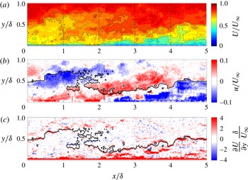
For visualisation, the PIV data were extended beyond the experimental field of view to allow for study of the scales of interest. Following the work of Zaman & Hussain (Reference Zaman and Hussain1981), a fixed convection velocity was used to ‘convect’ the PIV snapshots. Zaman & Hussain (Reference Zaman and Hussain1981) noted that, in the case of an isolated coherent structure in a turbulent flow, convecting the full shear flow with a single convection velocity equal to the centreline velocity of the structure maintained the closest approximation to the later shape of the structure. Figure 1 shows the extended visualisation of the instantaneous streamwise velocity and its wall-normal derivative. This work focuses on a particular structure, observable as large inclined features in the fluctuating streamwise velocity field of figure 1(b). The centreline velocity of this structure,
 $0.8U_{\infty }$
, was used as the visualisation convection velocity to minimise any distortion.
A visualisation of the instantaneous streamwise velocity is shown from PIV data in the wall-normal–streamwise plane. Contours of the velocity field in the laboratory frame are shown in (a) at the values
 $U/U_{\infty }=0:0.05:1$
, with every other isocontour outlined in black for visual clarity. A single isocontour of the laboratory frame velocity field
 $U/U_{\infty }=0.8$
is overlaid on (b,c) to illustrate the relationship between panels. Contours of the fluctuating velocity field are shown in (b) at the values
 $u/U_{\infty }=-0.15:0.01:0.15$
in the wall-normal–streamwise plane. The wall-normal derivative of the laboratory frame velocity field is shown in (c) at values of
 $(\unicode[STIX]{x2202}U/\unicode[STIX]{x2202}y)(\unicode[STIX]{x1D6FF}/U_{\infty })=-4:0.4:4$
. The dashed lines in (a) demarcate data used for the histograms of figure 3. The flow moves from left to right.

The fluctuating amplitude of the structure observed in figure 1 was approximated for use in constructing a model of LSMs. To isolate the large-scale structure, the Reynolds-decomposed streamwise velocity data within
 $3<x/\unicode[STIX]{x1D6FF}<4.5$
,
 $0<y/\unicode[STIX]{x1D6FF}<1$
of figure 1(b) were filtered with a Gaussian filter with standard deviation
 $0.5\unicode[STIX]{x1D6FF}$
. The fluctuating amplitude was defined as half of the peak-to-peak amplitude of the filtered field and was found to be
 $0.12U_{\infty }$
. A 20 % increase in filter size led to a 12 % decrease in the peak-to-peak amplitude calculated. It should be noted that the filtering procedure was used to find the amplitude of the large-scale structure, and was not used for visualisation in figure 1.
3 Modelling an LSM
A Reynolds decomposition was applied to the complete streamwise velocity field,
 $U$
, such that
 $U(x,y,z,t)=\bar{U}(x,y)+u(x,y,z,t)$
where
 $\bar{U}$
is the temporal mean of the flow field and
 $u$
represents the fluctuation about that mean. The fluctuation was further decomposed into a particular scale chosen to represent LSMs,
 $\tilde{u}$
, and other fluctuations that are not coherent at that scale,
 $u^{\prime }$
, to arrive at a triple decomposition
 $U(x,y,z,t)=\bar{U}(x,y)+\tilde{u}(x,y,z,t)+u^{\prime }(x,y,z,t)$
(Hussain & Reynolds Reference Hussain and Reynolds1970; Jacobi & McKeon Reference Jacobi and Mckeon2011). The scale of interest,
 $\tilde{u}$
, may be identified from experimental or computational data by filtering, conditionally averaging on a strong event or performing a modal analysis.
For simplicity in the model, the mean velocity field was assumed to be constant in the streamwise direction,
 $\bar{U}=\bar{U}(y)$
, invoking the parallel flow assumption for turbulent boundary layers. While boundary layers do not strictly obey this assumption, the wavenumbers of LSMs in channels, pipes and boundary layers are extremely similar (Monty et al.
Reference Monty, Hutchins, Ng, Marusic and Chong2009), suggesting that a model derived from a parallel flow framework may be useful across all three geometries. The LSM representative model was constructed to take the form of a travelling wave in the fluctuating velocity field, periodic in both the streamwise,
 $x$
, and spanwise,
 $z$
, directions. This choice of representation allowed for a clear connection between the model and the streamwise velocity spectrum, as the model could be associated with a single point in streamwise and spanwise frequency space. Right and left propagating waves were summed to isolate a downstream propagating wave,
 $$\begin{eqnarray}\tilde{u}(x,y,z,t)=\text{Re}(\hat{u}(y)(\text{e}^{\text{i}(k_{x}x+k_{z}z-\unicode[STIX]{x1D714}t)}+\text{e}^{\text{i}(k_{x}x+(-k_{z})z-\unicode[STIX]{x1D714}t)})),\end{eqnarray}$$
where
 $k_{x},k_{z}$
and
 $\unicode[STIX]{x1D714}$
are the streamwise, spanwise and temporal wavenumbers respectively and
 $\text{Re}$
indicates the real part.
For this study, a characteristic streamwise wavelength of
 $4\unicode[STIX]{x1D6FF}$
was chosen to align with observations of LSMs in the streamwise energy spectra of pipes, channels and boundary layers (Monty et al.
Reference Monty, Hutchins, Ng, Marusic and Chong2009). A spanwise wavelength of
 $1\unicode[STIX]{x1D6FF}$
was chosen to match the measured coherence of LSMs (Kovasznay et al.
Reference Kovasznay, Kibens and Blackwelder1970) and a convection velocity of
 $0.8U_{\infty }$
was chosen to place the structure in an appropriate region of the flow. To determine the wall-normal coherence of the model,
 $\hat{u}(y)$
, the resolvent formulation for wall-bounded turbulent flows was used for the boundary layer geometry with a parallel flow assumption (McKeon & Sharma Reference Mckeon and Sharma2010; Jacobi & McKeon Reference Jacobi and Mckeon2011). Fourier transforms in the streamwise, spanwise and temporal variables isolated the wall-normal coherence as the output of the formulation.
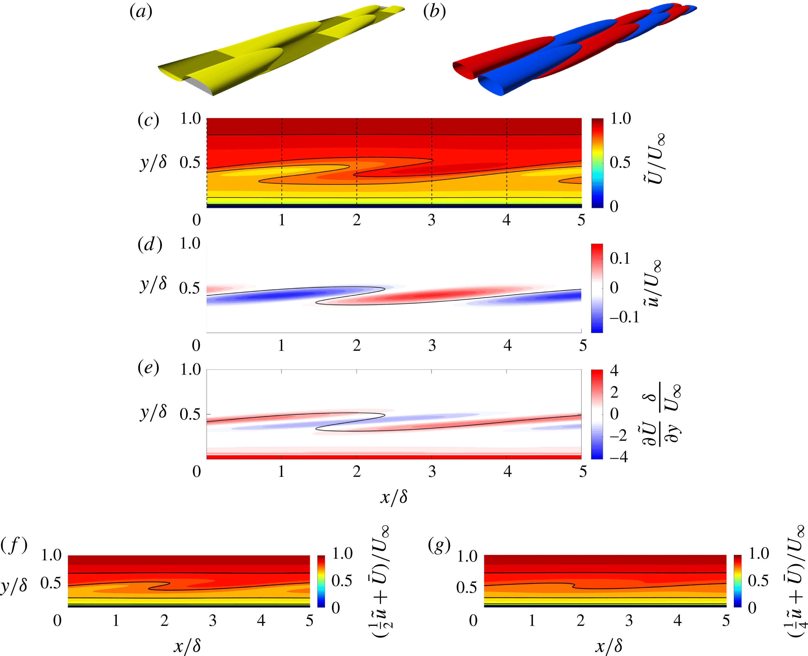
The structure of the LSM representative model is shown for the laboratory frame streamwise velocity field
 $\tilde{U}$
and the fluctuating velocity field
 $\tilde{u}$
. Three-dimensional representations of streamwise velocity isosurfaces are shown in (a) for
 $\tilde{U}/U_{\infty }=0.8$
(yellow) and
 $\bar{U}/U_{\infty }=0.8$
(black), and in (b) for
 $\tilde{u}/U_{\infty }=0.03$
(red) and
 $-0.03$
(blue). In (c), a wall-normal–streamwise slice of the laboratory frame velocity field is shown with the contour range
 $\tilde{U}/U_{\infty }=0:0.05:1$
and every other isocontour outlined in black for visibility. A single isocontour of
 $\tilde{U}/U_{\infty }=0.8$
is overlaid on (d,e) to illustrate the relationship between panels. Contours of the fluctuating velocity field are shown in (d) at the values
 $\tilde{u}/U_{\infty }=-0.15:0.01:0.15$
, while the wall-normal derivative of
 $\tilde{U}$
is shown in (e) at the values
 $(\unicode[STIX]{x2202}\tilde{U}/\unicode[STIX]{x2202}y)(\unicode[STIX]{x1D6FF}/U_{\infty })=-4:0.4:4$
. The laboratory frame streamwise velocity field (same contour values as c) is shown with the fluctuating amplitude of the LSM representative model halved in (f) and quartered in (g). The dashed lines in (c) demarcate data used for the histograms of figure 3. The flow moves from left to right.

Resolvent analyses formulate the Navier–Stokes equations as an input–output system between an input forcing and the velocity field, with the linear dynamics acting as a transfer function between the two. The linear transfer function is termed the resolvent operator,
 $\boldsymbol{{\mathcal{H}}}$
. A singular value decomposition was performed on the resolvent operator to determine the right (
 $\unicode[STIX]{x1D731}$
) and left (
 $\unicode[STIX]{x1D733}$
) singular vectors for each wavenumber triplet (streamwise, spanwise and temporal). In this formulation,
 $\boldsymbol{{\mathcal{H}}}(k_{x},k_{z},\unicode[STIX]{x1D714})=\unicode[STIX]{x1D733}\unicode[STIX]{x1D72E}\unicode[STIX]{x1D731}$
, where
 $\unicode[STIX]{x1D72E}$
is the matrix of singular values. The operator has been observed to be low rank (McKeon & Sharma Reference Mckeon and Sharma2010), such that the first singular vector is much more amplified by the linear dynamics at a given wavenumber triplet than the second singular vector. For the selected wavenumber triplet, the first two singular values were found to be
 $\unicode[STIX]{x1D70E}_{1}=36.4$
and
 $\unicode[STIX]{x1D70E}_{2}=2.0$
. The first singular vector was used as an approximation of the wall-normal coherence for the model, such that
 $\hat{u}(y)=\unicode[STIX]{x1D712}\unicode[STIX]{x1D713}(y)$
, where
 $\unicode[STIX]{x1D712}$
is the weighting of the mode and
 $\unicode[STIX]{x1D713}$
is the first singular vector. The wavenumber of this structure is not expected to vary substantially with the Reynolds number, as energetic regions associated with LSMs have been identified at similar streamwise wavelengths in the streamwise energy spectra across many Reynolds numbers (Monty et al.
Reference Monty, Hutchins, Ng, Marusic and Chong2009; Rosenberg et al.
Reference Rosenberg, Hultmark, Vallikivi, Bailey and Smits2013). The scaling with the Reynolds number of the singular value and geometry of modes in the outer region is reported by Moarref et al. (Reference Moarref, Sharma, Tropp and Mckeon2013), while the scaling of the full weighting
 $\unicode[STIX]{x1D712}$
is the subject of ongoing work. A data-based approach was used to approximate
 $\unicode[STIX]{x1D712}$
at an
 $Re_{\unicode[STIX]{x1D70F}}$
of 910. Using the filtering method described in § 2, the peak-to-peak amplitude of the large-scale structure of figure 1 was computed. Half of this peak-to-peak amplitude was used as the fluctuating amplitude of the LSM representative model,
 $\max (\hat{u})=\unicode[STIX]{x1D712}$
. The value of
 $\unicode[STIX]{x1D712}$
was identified as
 $\unicode[STIX]{x1D712}/U_{\infty }=0.12$
.
Figure 2(a,b) shows the three-dimensional structure of the LSM representative model with the mean (
 $\tilde{U}\equiv \bar{U}+\tilde{u}$
) and without the mean velocity field superimposed (
 $\tilde{u}$
) respectively. In (a), the streamwise velocity isocontour is seen to alternate between protruding above and protruding below its mean position, giving the appearance of bulges. In (b), the structure is observed to be periodic in the streamwise and spanwise directions, with a compact wall-normal coherence and a phase change of
 $\unicode[STIX]{x03C0}$
across its height. To compare the model and the data, any velocity field that includes the mean will be referred to as a laboratory frame velocity field, while the velocity fields that do not include the mean will be referred to as fluctuating velocity fields. This is done with acknowledgement of the distinction between the PIV data, which include the fluctuations that are not coherent with the scale of interest, and the velocity field of the model, which does not include
 $u^{\prime }$
.
4 Results and discussion
4.1 Connecting the streamwise energy spectrum to bulges
The structure of the LSM representative model in the wall-normal–streamwise plane (figure 2 c–e) is seen to compare favourably with that of the instantaneous structure observed in the unfiltered PIV data of figure 1. In figures 1 and 2, equally strong positive and negative inclined structures are observed in the fluctuating streamwise velocity field, while a bulge is observed in the laboratory frame velocity field. In the laboratory frame velocity field, a positive fluctuating structure corresponds to the absence of a visible structure (downward protrusion of isocontours), and the streamwise length scale of the structure, which is constant in the fluctuating field, is observed to change as a function of the wall-normal height.
The amplitude of the LSM representative model was deduced from a single frame of PIV, and is therefore the largest source of uncertainty in the model. Figure 2(f,g) demonstrates the effect on the laboratory frame velocity field of halving and quartering the fluctuating amplitude of the LSM representative model relative to its strength in figure 2(d). The presence of an asymmetric bulge shape is consistent through these large changes in fluctuating amplitude, but changes in the apparent height, width and inclination angle of the laboratory frame velocity structure are observed.
The black curves in figures 1 and 2 represent the heights of the laboratory frame streamwise velocity isocontours,
 $h_{U}(x,z,t)$
, defined as the set of wall-normal locations where the laboratory frame streamwise velocity field is equal to some particular value,
 $U(x,h_{U},z,t)=U^{\ast }$
. The analytical relationship between a laboratory frame streamwise velocity isocontour and the fluctuating velocity field can be derived to clarify the trends observed in figures 1 and 2. The height of the mean streamwise velocity isocontour,
 $h_{\bar{U}}(x)$
, is defined as the set of wall-normal locations where the mean velocity field is equal to the same value,
 $\bar{U}(x,h_{\bar{U}})=U^{\ast }$
, where
 $x$
-dependence of the mean is retained for generality in the following derivation. In general, fluctuations relative to a mean appear in laboratory frame velocity isocontours as differences between
 $h_{U}$
and
 $h_{\bar{U}}$
. The relationship between a fluctuating velocity field,
 $u(x,y,z,t)$
, and the change in laboratory frame isocontour height,
 $\unicode[STIX]{x0394}h_{U}\equiv h_{U}-h_{\bar{U}}$
, can be defined for laboratory frame velocity fields with monotonic variation in
 $y$
(equivalently
 $|\unicode[STIX]{x2202}u/\unicode[STIX]{x2202}y|<\unicode[STIX]{x2202}\bar{U}/\unicode[STIX]{x2202}y$
) by expanding
 $U$
in a Taylor series about the height
 $h_{\bar{U}}$
,
 $$\begin{eqnarray}\unicode[STIX]{x0394}h_{U}(x,z,t)=h_{U}(x,z,t)-h_{\bar{U}}(x)\approx -\left[u\left/\left(\frac{\unicode[STIX]{x2202}U}{\unicode[STIX]{x2202}y}\right)\right.\right]_{(x,h_{\bar{U}},z,t)}.\end{eqnarray}$$
In a geometry where the mean shear is defined as positive, (4.1) demonstrates that a negative velocity fluctuation corresponds to an upward protrusion of the laboratory frame isocontour relative to its position in the mean velocity field, while a positive fluctuation is consistent with a downward protrusion of the isocontour. Although the monotonic condition on
 $U$
does not hold everywhere in figures 1 and 2, the relationship between the height of the laboratory frame velocity isocontours and the sign of the fluctuating velocity structures can still be observed. From (4.1), one also sees that the strength of the wall-normal derivative of the laboratory frame streamwise velocity field or ‘shear’ field is inversely proportional to the isocontour height change. This relationship coupled with the consistent spatial relationship between the velocity and shear fields leads to gradual increases in isocontour height with
 $x$
, known as ‘ramps’, and rapid decreases in isocontour height with
 $x$
, known as ‘cliffs’, in the laboratory frame velocity fields of the model and the data.
Equation (4.1) sheds light on a fundamental equivalency between symmetry in the fluctuating velocity field and asymmetry in the laboratory frame velocity field that allows the statistical and structural perspectives to be consistent and representable by the LSM representative model. This equivalency also clarifies the focus on low-speed structures in the structural turbulence community. Fluctuating structures with amplitude less than the mean correspond to visually identifiable bulges in the isocontours of the laboratory frame streamwise velocity field. The fluctuating structures with amplitude larger than the mean have an equally strong relationship with the shape of the laboratory frame isocontours, but their impact (the downward protrusion of isocontours) is less visually identifiable.
4.2 Connecting the streamwise energy spectrum to UMZs
The LSM representative model also reproduces the UMZ behaviour observed by Meinhart & Adrian (Reference Meinhart and Adrian1995) using the instantaneous streamwise velocity histogram technique. In this technique, a discrete approximation of the probability density function of an instantaneous laboratory frame streamwise velocity field is calculated, identifying the most and least common velocity values in the instantaneous field. Instantaneous streamwise velocity histograms of turbulent boundary layers have been shown to have discrete minima and maxima, which have been correlated to the presence of regions of almost constant velocity (UMZs) bordered by thin regions of rapidly changing velocity (shear layers) (Adrian et al. Reference Adrian, Meinhart and Tomkins2000b ; de Silva et al. Reference de Silva, Hutchins and Marusic2016).
This histogram technique was applied to the experimental data and the LSM representative model over four different streamwise ranges. The dashed lines in figures 1(a) and 2(c) demarcate the regions of data used for the histograms, although the equivalent spatial data from the appropriate instantaneous snapshot were used for the experimental histograms, rather than the temporally reconstructed representation shown in figure 1(a). The histograms were calculated using a
 $1\unicode[STIX]{x1D6FF}$
range in the streamwise direction and 50 velocity bins, with the free stream masked following the procedure of de Silva et al. (Reference de Silva, Hutchins and Marusic2016). The turbulent/non-turbulent interface (TNTI) was identified using a turbulence intensity threshold (Chauhan et al.
Reference Chauhan, Philip, de Silva, Hutchins and Marusic2014) with a value of
 $k_{th}=0.5$
for the PIV data and
 $k_{th}=3.5$
for the model. These values of
 $k_{th}$
were chosen such that the mean height of the TNTI,
 $\bar{Y}/\unicode[STIX]{x1D6FF}$
, was 0.82 for both the PIV and the LSM representative model, matching previous studies (Chen & Blackwelder Reference Chen and Blackwelder1978). The modelled and experimental velocity fields were represented on identical grids for the calculation of the histograms.
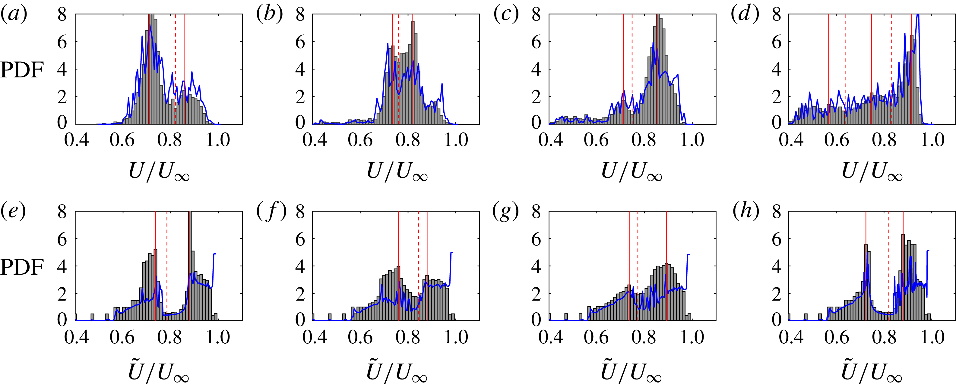
At least two distinct maxima are present in each histogram, shown in figure 3, indicating UMZ behaviour in the laboratory frame velocity field of the data and the model (Adrian et al.
Reference Adrian, Meinhart and Tomkins2000b
). Good agreement is seen in the locations of local maxima at
 $U/U_{\infty }\approx 0.7$
and
 $U/U_{\infty }\approx 0.9$
and the location of a local minimum at
 $U/U_{\infty }\approx 0.8$
in all panels other than (b) and (f). Less favourable agreement is seen in the amplitude of the peaks. In (a,e) and (d,h), reasonable agreement is seen for the amplitude of one of the peaks (
 $U/U_{\infty }\approx 0.7$
and
 $U/U_{\infty }\approx 0.9$
respectively), while poor agreement is seen for the amplitude of the other. In (b,f), little agreement is seen, while in (c,g), the amplitudes of both peaks show some agreement. In addition, activity is observed at low streamwise velocity values in the PIV data of (c,d) that is not seen in the model, probably indicating the influence of a VLSM. Although additional work is needed to achieve quantitative prediction, figure 3 demonstrates that periodic symmetric structures in the fluctuating velocity field can yield physically realistic UMZ behaviour in the laboratory frame velocity field, allowing UMZs and the spectral description of LSMs to be compatible.
Histograms of the laboratory frame streamwise velocity field of instantaneous PIV data
 $U$
(a–d) and the LSM representative model
 $\tilde{U}$
(e–h). The histograms are derived from data in figures 1(a) and 2(c) in the streamwise ranges (a,e)
 $0<x/\unicode[STIX]{x1D6FF}<1$
, (b,f)
 $1<x/\unicode[STIX]{x1D6FF}<2$
, (c,g)
 $2<x/\unicode[STIX]{x1D6FF}<3$
and (d,h)
 $3<x/\unicode[STIX]{x1D6FF}<4$
. The solid red lines indicate local maxima in the histograms, while the dashed red lines indicate local minima. The blue curves represent an estimate of the probability density function derived from the wall-normal derivative of the streamwise velocity field (4.4).

Previous interpretations of the instantaneous streamwise velocity histograms have argued that maxima in the histograms indicate modal velocities of UMZs, while minima indicate shear layers (Adrian et al. Reference Adrian, Meinhart and Tomkins2000b ). A derivation of the exact probability density function for a streamwise velocity profile clarifies this relationship and identifies a direct relationship between the instantaneous streamwise velocity histogram and the shear field.
A laboratory frame streamwise velocity profile is considered at a single streamwise, spanwise and temporal location:
 $U(x_{0},y,z_{0},t_{0})\equiv U_{0}(y)=G(y)$
. As a simplification, it is assumed that
 $G$
is one to one, such that one can write down the inverse relationship
 $y=G^{-1}(U_{0})$
(this is equivalent to the monotonic assumption of § 4.1). Then, the probability density function for the instantaneous velocity profile,
 $U_{0}(y)$
, can be analytically written as
 $$\begin{eqnarray}f(U_{0})=\frac{\text{d}}{\text{d}U_{0}}\left(\int _{-\infty }^{G^{-1}(U_{0})}\unicode[STIX]{x1D719}(y)\,\text{d}y\right),\end{eqnarray}$$
where
 $f$
is the probability density function of
 $U_{0}$
and
 $\unicode[STIX]{x1D719}$
is the probability density function of
 $y$
. For
 $y$
uniformly distributed between two points
 $y_{i}$
and
 $y_{f}$
(a uniform grid), one can show that
 $$\begin{eqnarray}f(U_{0})=\frac{c}{{\displaystyle \frac{\unicode[STIX]{x2202}U}{\unicode[STIX]{x2202}y}}(x_{0},G^{-1}(U_{0}),z_{0},t_{0})},\end{eqnarray}$$
where
 $c=1/(y_{f}-y_{i})$
.
Equation (4.3) demonstrates that the probability density function of an instantaneous streamwise velocity profile is the inverse of the local shear with a scaling. This matches the intuitive reasoning of Adrian et al. (Reference Adrian, Meinhart and Tomkins2000b
): maxima in a histogram correspond to low-shear events, while minima correspond to high-shear events. The inverse function
 $y=G^{-1}(U_{0})$
builds in the idea of locality, requiring that one consider the shear and the velocity at the same point in space. It should be noted that this simplified analysis was performed at a single streamwise and spanwise location because a larger-dimensional analysis would complicate the definition of the inverse relationship.
When
 $G$
is not one to one, the relationship highlighted by (4.3) retains predictive value. A few modifications are necessary to apply the derived equation to turbulent data, where the magnitude of the local shear can be much larger than that of the mean shear: one must constrain the relationship between the wall-normal coordinate and the streamwise velocity value; the absolute value of the shear must be considered rather than its signed value; and, to compare with histograms reported in the literature (Adrian et al.
Reference Adrian, Meinhart and Tomkins2000b
; de Silva et al.
Reference de Silva, Hutchins and Marusic2016) and those shown in figure 3, one must approximate the probability density function over a two-dimensional region of the flow. As an estimate for the 2D probability density function, one can average the probability density function of all measured profiles across a 1
 $\unicode[STIX]{x1D6FF}$
range in
 $x$
, consistent with the data range used for the histograms in figure 3. Then,
 $$\begin{eqnarray}f(U_{2D})\approx \frac{1}{N}\mathop{\sum }_{i=1}^{N}\frac{c}{\left|{\displaystyle \frac{\unicode[STIX]{x2202}U}{\unicode[STIX]{x2202}y}}(x_{i},g^{-1}(U_{i}),z_{0},t_{0})\right|},\end{eqnarray}$$
where
 $N$
is the number of streamwise locations considered,
 $U_{i}$
is the velocity profile at a given streamwise location
 $x_{i}$
and
 $y=g^{-1}(U_{i})$
is the modified inverse relationship. For the present work,
 $y=g^{-1}(U_{i})$
is defined as the height where the instantaneous velocity profile is closest to the input velocity value. If there is no height where the velocity profile is within 1 % of the input velocity value,
 $f(U_{2D})$
is set to zero. This definition of
 $g^{-1}$
is found to be a unique mapping in the discrete velocity fields. The result of applying (4.4) to the PIV data and the LSM representative model is shown in figure 3 and is seen to closely match the directly computed histograms, suggesting that the histograms are a measure of local shear in the flow, as intuited by Adrian et al. (Reference Adrian, Meinhart and Tomkins2000b
). The largest discrepancies between the computed histograms and the approximated probability density function are observed at the largest values of the probability density function, where the shear is lowest and the assumption of uniqueness of the velocity field is least valid.
Given that a model of a single scale can reproduce two UMZs, the superposition of a very small number of such models could lead to the three to five UMZs observed across
 $Re_{\unicode[STIX]{x1D70F}}=$
 $10^{3}$
–
 $10^{4}$
by de Silva et al. (Reference de Silva, Hutchins and Marusic2016). In considering which other scales to include, the travelling wave formulation of the model allows one to turn to the energy spectrum for guidance. The scale chosen for this study was one out of a narrow band of energetic scales associated with LSMs. The wall-normal structure of the scales in this energetic band is essentially uniform, with a wall-normal thickness that varies slightly with a critical layer scaling (McKeon & Sharma Reference Mckeon and Sharma2010). Superposition of a few scales that are dominant in the energy spectrum, e.g. from the LSM energy band, the superstructures or VLSMs and the near-wall cycle, would lead to a modelled flow that is compatible with the energetic features of real wall-bounded flows. Superposition of multiple modes can also be used to allow for the representation of more complex phenomena, such as the meandering of structures (Sharma & McKeon Reference Sharma and Mckeon2013) and amplitude modulation of small scales (McKeon Reference Mckeon2017).
5 Conclusion
A representative model for LSMs in wall-bounded turbulent flows was developed, with scale information from the streamwise energy spectrum and wall-normal coherence information from the Navier–Stokes equations. The model was found to naturally capture key structural characteristics of LSMs, including bulges in the isocontours of the laboratory frame streamwise velocity field and distinct minima and maxima in the instantaneous streamwise velocity histograms, indicating UMZ behaviour. The success of this simple model was argued to demonstrate the equivalence of the LSMs of the energy spectrum and the bulges and UMZs of the instantaneous velocity fields.
A key observation towards connecting the statistical and instantaneous descriptions was the reconciliation of the characteristics of the fluctuating and laboratory frame streamwise velocity fields in which they were respectively described. Visualisations of the LSM representative model highlighted a non-trivial relationship between the instantaneous fluctuating and laboratory frame velocity fields: symmetry in high- and low-momentum structures and constant streamwise length scales were observed in the fluctuating field, while asymmetry between high- and low-momentum structures and varying streamwise length scales were observed in the laboratory frame field. These observations were explained through the development of an analytic expression for the shape of a laboratory frame streamwise velocity isocontour given a fluctuating velocity field. Connection of the statistical description to the UMZ behaviour required the use of the instantaneous streamwise velocity histogram technique, which has been used to identify UMZ behaviour in previous work (Adrian et al. Reference Adrian, Meinhart and Tomkins2000b ; de Silva et al. Reference de Silva, Hutchins and Marusic2016). This technique was analysed by considering the probability density function of a streamwise velocity profile and was shown to be a direct measure of the local shear field.
The success of the LSM representative model supports the use of a travelling wave to understand and model turbulent structures (Sharma & McKeon Reference Sharma and Mckeon2013). Travelling wave models can act as a bridge between statistics and instantaneous fields: their periodicity allows for a direct connection to spectral descriptions of turbulent statistics, while their wall-normal coherence allows for a direct connection to the instantaneous flow features. Future work will consider the superposition and interaction of multiple representative models, towards capturing trends in the number of UMZs with Reynolds number and capturing multi-scale instantaneous features such as hairpin packets.
Acknowledgements
This work was made possible through the support of a National Defense Science and Engineering Graduate (NDSEG) Fellowship and United States Air Force grants FA9550-12-1-0060 and FA9550-16-1-0361. The authors would like to thank Dr S. Dawson for his work on the boundary layer resolvent code.