

Predicting driving outcomes in older drivers has been the focus of several important studies (Ball et al., Reference Ball, Roenker, Wadley, Edwards, Roth and McGwin2006; O’Connor, Kapust, Lin, Hollis, & Jones, Reference O’Connor, Kapust, Lin, Hollis and Jones2010; Marshall et al., Reference Marshall, Man-Son-Hing, Bédard, Charlton, Gagnon and Gélinas2013; Staplin, Lococo, Gish, & Decina, Reference Staplin, Lococo, Gish and Decina2003; Wood, Anstey, Kerr, Lacherez, & Lord, Reference Wood, Anstey, Kerr, Lacherez and Lord2008). The overarching goal of these endeavors has been to develop and validate off-road assessment instruments, such as performance based tests, that can predict whether an older driver may be at risk of engaging in unsafe driving behaviours. The approach taken to tackle this issue varies greatly across studies. While some studies examined driving performance across various performance domains ranging from visual acuity to neck flexibility (e.g., Wood et al., Reference Wood, Anstey, Kerr, Lacherez and Lord2008), others have focused on evaluating the sensitivity of specific instruments, such as indices of general cognitive impairment (e.g., Bédard et al., Reference Bédard, Marshall, Man-Son-Hing, Weaver, Gélinas and Korner-Bitensky2013; Dobbs & Schopflocher, Reference Dobbs and Schopflocher2010). The results of these assessments are then typically compared to one or more driving outcomes such as on-road test performance, crashes and traffic violations, and driving simulator performance (Kay, Bundy, Clemson, Cheal, & Glendenning, Reference Kay, Bundy, Clemson, Cheal and Glendenning2012). Ultimately, the goal is to provide health practitioners and licensing authorities with a valid assessment system that can accurately determine fitness to drive.
A critical factor of such research is whether the findings of the study, or more explicitly its external validity, can be generalized to the broader population of older drivers. Stakeholders, including government representatives, physicians, and most importantly, older drivers themselves, need to be assured that the outcomes of a given method of assessment accurately reflect fitness to drive (Kay et al., Reference Kay, Bundy, Clemson, Cheal and Glendenning2012; Marshall et al., Reference Marshall, Man-Son-Hing, Bédard, Charlton, Gagnon and Gélinas2013) and are applicable to them.
One key methodological consideration to ensure that an assessment of fitness to drive can be extended to the general population is the representativeness of the sample used to develop the driving assessment battery. In an ideal methodological study design, probability (i.e., random) sampling methods or mandatory participation are technically the only recognized approaches that will lead to the creation of representative samples of the general population (Cochran, Reference Cochran1951; Cochran, Mosteller, & Tukey, Reference Cochran, Mosteller and Tukey1954; Marshall, Reference Marshall1996). However, this type of sampling strategy is not feasible for the purpose of studying driving safety in older drivers. For obvious ethical reasons, mandatory participation is not a viable option. On the other hand, random sampling would require the recruitment of a sufficiently large number of participants from all geographical regions of a given country who would be randomly selected to participate in the study.
To our knowledge, no study to date on driving in older adulthood has recruited what could be methodologically termed a representative sample of the population. Indeed, the inherent complexity of such investigations has forced researchers to use convenience sampling as the best possible alternative. Furthermore, the design and complexity of any study on driving will vary according to the outcomes of interest (e.g., on-road performance, crash risk), the breadth and depth of the assessment process used, the duration of participant follow-up (i.e., months to multiple years), and the use of single or multiple testing sites. The success of any recruitment strategy will depend on these factors as well as on the potential implications for the participants, such as suspension of one’s driving license.
Selecting on-road performance as a key driving outcome increases the complexity and the cost of a study. Additionally, this could influence the recruitment success rate, resulting sample size, and possibly the representativeness of the sample. Wood et al. (Reference Wood, Anstey, Kerr, Lacherez and Lord2008) conducted such a study on older community dwellers in Queensland, Australia, using the electoral roll to recruit participants. They managed to recruit 272 older participants aged 70 and older for a success rate of only 11 per cent.
However, the recruitment rate of participants can be increased under proper circumstances. In a very influential study linking the risk of a crash to performance-based tests, Ball et al. (Reference Ball, Roenker, Wadley, Edwards, Roth and McGwin2006) recruited 1,910 individuals who visited a department of motor vehicles (DMV) office in Maryland for the purpose of renewing their license. Participants were recruited at three DMV sites. The high recruitment rate of 48 per cent was influenced by the fact that participation had no bearing on driving privileges, testing was limited to one session that was performed on-site, and the driving outcome of interest was motor vehicle collisions as opposed to on-road performance.
More recently, Emerson et al. (Reference Emerson, Johnson, Dawson, Uc, Anderson and Rizzo2012) recruited 100 drivers aged 65 and older from the Iowa area to participate in a study that aimed to predict several driving outcomes including driving cessation, crash, or moving violations. On-road driving performance was also assessed. The convenience sample was recruited from the community using various types of announcements and advertisements, an approach that is considered rather typical for research on driving and aging.
Although a randomized selection of participants increases the likelihood of building a representative sample, self-selection and geographical limitations of the study, such as evidenced in work by Wood et al. (Reference Wood, Anstey, Kerr, Lacherez and Lord2008), may also jeopardize the representativeness of a sample. For instance, the process of self-selection can result in the following biases: (1) drivers who volunteer may be more skilled at driving or at least have more confidence in their level of driving skill; and (2) drivers with health problems that negatively impact on driving abilities may be less likely to volunteer not only due to possibly decreased ability, but also due to energy and eagerness to participate in a research study.
Therefore, the external validity of findings from previous studies on fitness to drive that employed convenience sampling, or even random samples that are geographically limited, may be put into question if the representativeness of the sample remains unknown. Unfortunately, none of the studies on the prediction of driving outcomes in older drivers provide adequate information that would support the representativeness of the selected sample. Ideally, for this to be done, the sample would have to be compared to the general population of older drivers across several parameters, and this is only achievable if such data for the population is available.
The goal of the present study was to examine the representativeness of the convenience sample of drivers age 70 and older taking part in the Candrive II prospective cohort study.
Demographic, health, and functional status variables were used to assess whether the participants within the Candrive II study were representative of the broader Canadian population of older drivers (i.e., the Canadian Community Health Survey – Healthy Aging; CCHS-HA). We statistically compared the two samples using equivalence testing procedures (Cribbie, Gruman, & Arpin-Cribbie, Reference Cribbie, Gruman and Arpin-Cribbie2004). We hypothesized that Candrive II participants would be very similar on demographic and health parameters to participants from the larger CCHS-HA.
Methods
The data for the study were drawn from the following two datasets: Candrive II longitudinal study on older drivers’ baseline data and the CCHS-HA (Statistics Canada, 2008).
CIHR Candrive II Study of the Older Driver
The Candrive II study is a multicentre prospective cohort study that examines the predictive validity of tools for assessing fitness to drive (Marshall et al., Reference Marshall, Man-Son-Hing, Bédard, Charlton, Gagnon and Gélinas2013). Candrive II follows a cohort of drivers aged ≥70 over 5 years. A total of 928 participants have been recruited in seven Canadian cities across four provinces. Participants underwent a comprehensive assessment at baseline and yearly thereafter, as well as a brief follow-up assessment at 4 and 8 months each year. An in-car device (OttoView-CD Data Logging Device, Persen Technologies, Winnipeg, MB) was installed in each participant’s vehicle to record driving exposure and behaviour. Driving records are obtained annually from licensing authorities to document and derive the main driving outcomes of this study: (a) at-fault crashes per kilometre driven and (b) traffic violations. The Candrive II study is unique owing to its size, duration, and partnerships with Canadian stakeholders and researchers abroad (see Marshall et al. [Reference Marshall, Man-Son-Hing, Bédard, Charlton, Gagnon and Gélinas2013], for a thorough description of the Candrive II longitudinal study).
Candrive II Sample
The Candrive II sample (n = 928; 578 males, 350 females) consists of volunteers recruited from the community over the course of 18 months, from April 2009 to November 2010 (Marshall et al., Reference Marshall, Man-Son-Hing, Bédard, Charlton, Gagnon and Gélinas2013). Participants were recruited through various advertisements and announcements and in response to interviews with the media. Some of the inclusion criteria for the Candrive II study were (1) having a valid driver’s license; (2) driving at least four times per week (active driver); and (3) aged 70 or older. Inclusion and exclusion criteria were described in full in Marshall et al. (Reference Marshall, Man-Son-Hing, Bédard, Charlton, Gagnon and Gélinas2013). Each of the seven sites was responsible for the recruitment of its participants and was free to customize its recruitment strategies. Participants were recruited in seven different metropolitan areas of Canada: Hamilton, Ontario; Ottawa, Ontario; Thunder Bay, Ontario; Toronto, Ontario; Montreal, Quebec; Winnipeg, Manitoba; and Victoria, British Columbia.
CCHS-HA Sample
The CCHS-HA is a population-based, cross-sectional computer-assisted interview survey of Canadian respondents aged 45 and older residing in households (n = 28307; 12,253 males, 16,054 females), in all 10 provinces. The CCHS-HA excluded individuals living on reserves and other Aboriginal settlements, full-time members of the Canadian Forces, and persons living in collective dwellings and the institutionalized population. The exclusions represented approximately 4 per cent of the target population. The CCHS Healthy Aging study data were collected in the years 2008–2009. The Canadian population from which the sample was drawn was based on the 2006 Canadian census. All Canadian families containing at least one individual aged 45 and older in 2008 were part of the sample population. Representativeness of the sample was assured through a complex multi-step sample creation. Sampling units (number of participants) were allocated to all provinces to assure a minimal number of units, followed by a proportional allocation of units to each province according to the size of the sampling population in that province. In each province, the sampling units were also allocated proportionally according to urban and rural strata. City and urban clusters were created in such a way that a minimal number of household members aged 75 and older would be potentially included in the sample. All data were self-reported using computer-assisted personal interviewing, and data collection took place from December 1, 2008 until November 30, 2009. The response rate was over 75 per cent (household and person). A description of the design, sample, and interview protocol of the survey can be found in the CCHS-HA user guide at Statistics Canada (Statistics Canada, 2008). The CCHS-HA includes a number of variables related to respondents’ transportation habits among older adults. Turcotte (Reference Turcotte2012), for example, used data from the CCHS to provide a descriptive analysis of the transportation habits of older Canadians stratified by variables such as geographic location, sex, and age group.
For the purpose of conducting equivalence tests between the participants from the CCHS-HA sample and the Candrive II sample, only respondents aged 70 and older and who reported driving at least once a week were selected from the CCHS-HA database. The selection of these respondents from the CCHS-HA sample corresponds to the inclusion criteria for the aforementioned Candrive II study. In the entire CCHS-HA sample of adults aged 70 or older, 60 per cent reported driving a motor vehicle as their most common form of transportation; 79 per cent of older men and 44 per cent of older women drove. The final sample size from the CCHS-HA comprised 3,899 older drivers (2,278 males, 1,621 females). All data from the CCHS-HA were weighted to account for the effects of the multistage complex sample design.
Selection of Variables
The variables that we describe here are those that were common to both studies and that were comparable after no or minimal recoding. Two independent investigators reviewed the two datasets to find comparable variables. Variables were excluded from the analysis when both reviewers agreed that the variables were definitely not comparable. Decisions for recalculation or recoding were determined by the first author of this article. All the variables examined in the Candrive II and CCHS-HA studies have been thoroughly described elsewhere (Marshall et al., Reference Marshall, Man-Son-Hing, Bédard, Charlton, Gagnon and Gélinas2013; Statistics Canada, 2008); here, we detail only the variables that could be validly compared between the two samples. We used a two-step approach to select comparable variables. At the first step, we conducted a thorough review of the variables available in both studies to identify general topics (e.g., health, smoking, driving, functional status) that were present in both. At the second step, we determined whether the identified variables were assessed using the same instrument or scaling, or if recalculation could be achieved without affecting the scales. Unfortunately, many of the seemingly common variables collected in the two studies could not be validly compared, mostly due to the use of scaling approaches that were either incompatible or not sufficiently analogous to allow recoding of appropriate transformation of the data. For example, even though “smoking” is mentioned in both studies, CCHS has at least 24 different variables describing various types of smokers and stages of smoking cessations, whereas Candrive inquires about smoking only in two contexts: whether participants ever smoke while driving, and whether they have smoking-related problems; we did not find a valid way to recode smoking variables.
Demographic Variables
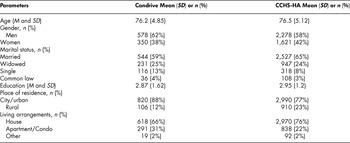
The demographic variables common to the CCHS-HA and Candrive II studies were age, gender, education, marital status, place of residence, and living arrangements (see Table 1). Marital status, living arrangements, and education required recoding. Place of residence had only two levels (urban or rural).
Socio-demographic characteristics of all drivers

CCHS-HA = Canadian Community Health Survey – Healthy Aging.
In Candrive II, marital status had 5 nominal categories (never married, married, common-law, separated/divorced, or widowed), while in the CCHS-HA study, participants had to select from six potential nominal categories (single, now married, common-law, separated, divorced, widowed). In order to make the variable marital status comparable, the single, separated, and divorced categories were collapsed in both studies. Consequently, we executed the analysis on a marital status variable that comprised four categories (single, married, common-law, or widowed).
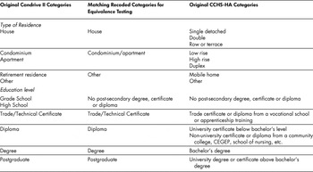
The original and recoded scales of residence type and education level are described in Table 2. For residence type, the variable that we used for comparisons had three levels: house, apartment/condominium, other. In the Candrive II study, the level of education was determined by asking participants “What is your highest level of education completed?”, with the offered categories being postgraduate, university degree, diploma, trade/technical certificate, high school, or grade school. In the CCHS-HA study, the question asked was somewhat different (“What is the highest degree, certificate or diploma you obtained?”) and the categories to choose from were as follows: (a) post-secondary degree, certificate, or diploma; (b) trade certificate or diploma from a vocational school or apprenticeship training; (c) non-university certificate or diploma (from a community college, school of nursing, etc.); (d) university certificate below bachelor’s level; (e) bachelor’s degree; or (f) university degree or certificate above bachelor’s degree. After recoding, the final scale had five levels: no post-secondary degree, trade/technical certificate, diploma, university degree, postgraduate.
Recoding of type of residence and education level

Health and Functional Status Variables
Eight health variables were found to be comparable between the two studies: self-perceived health, body mass index (BMI), height, weight, depression, and alcohol consumption. The last two variables required recoding, while the others were perfectly comparable as is. The activities of daily living (ADL) (Fillenbaum & Smyer, Reference Fillenbaum and Smyer1981; Razani et al., Reference Razani, Casas, Wong, Lu, Alessi and Josephson2007) and the instrumental activities of daily living (IADL) (Nourhashémi et al., Reference Nourhashémi, Andrieu, Gillette-Guyonnet, Vellas, Albarède and Grandjean2001; Tomaszewski et al., Reference Tomaszewski, Cahn-Weiner, Harvey, Reed, Mungas and Kramer2009) scales were both administered in the Candrive II study and the CCHS-HA study. Participants from both studies also indicated whether they were employed. Engagement in social activities was also questioned in both studies.
Participants’ self-rated health was compared using a single question on the SF-36, which was administered to the Candrive sample. Participants in both samples responded to the following question: “In general, would you say your health is …” and were given the following response choices: excellent, very good, good, fair, or poor. Candrive II study participants had their height and weight measured in person while in the CCHS-HA protocol, the height and weight of participants were self-reported. BMI was calculated for all participants using the following equation: weight (in kg)/height2 (m).
Depression was measured with the Geriatric Depression Scale (short form; Sheikh & Yesavage, Reference Sheikh, Yesavage and Brink1986) in the Candrive II study. The Geriatric Depression Scale (short form) includes 15 “yes” or “no” questions. Among the 15 questions, 10 suggest the presence of depression when answered positively, and the remaining five items indicate probability of depression when answered negatively. Participants with a score of 6 and above were considered likely to be depressed. The respective CCHS-HA variable was calculated from the score obtained on the Depression Scale – Short Form Score. The CCHS-HA Depression Scale – Short Form Score comprises 19 items which assess the depression level of respondents who felt depressed or lost interest in things for at least two weeks or more over the past year. The score from the depression scale was then expressed as a probability (expressed as a proportion) that the respondent would have been diagnosed as having experienced a major depressive episode in the past 12 months had they completed the Long-Form Composite International Diagnostic Interview. Respondents with a probability value of 0.9 or greater were considered likely to be depressed. Consequently, it was possible to categorize the participants from both samples as being depressed or not.
Alcohol consumption in Candrive II participants was assessed by the following question “Do you ever drink alcohol?” with possible answers being either “yes” or “no”. Following a positive response, participants were asked “On average how often do you drink?” with three possible options: daily basis, less than daily basis, or less than weekly. In CCHS-HA, participants were asked “During the past 12 months, how often did you drink alcoholic beverages?” Possible responses were as follows: less than once a month, once a month, 2 to 3 times a month, once a week, 2 to 3 times a week, 4 to 6 times a week, or every day. The CCHS-HA scale was recoded so that it matched the three-level response of the Candrive II scale: daily (every day in CCHS-HA); less than daily (4–6 times a week, 2 to 3 times a week, once a week in CCHS-HA); and less than weekly (once a month and less than once a month in CCHS-HA).
The ADL scale contains a total of seven activities that help to determine the level of independence in functioning. These activities include bathing, grooming, dressing, eating, transferring from a bed to a chair, using a toilet, and walking. Responses are of three types: “unable to do it” (0), “able to do it with some help” (1), or “without any help” (2). The items are summed to give a total ADL score ranging from 0 (major problems with ADLs) to 14 (no problems with ADLs). The IADL scale was also administered in both studies comprise seven activities, such as using the telephone; ability to get to places outside of walking distance; shopping; preparing meals; housework; ability to take own medicine; and ability to handle money. Responses are also on a 0 to 2 scale (completely unable, with some help, without any help), for a 0–14 total score range.
Responses to the employment question were either “yes” or “no” in both cohorts. Social participation in both samples was dichotomized in the following manner. It was coded as “yes, socially active” in CCHS if, in the past 12 months, a participant engaged in any of the following activities at least once a month or more often: family/friendship activities outside the household, church or religious activities, sports or physical activities, educational and cultural activities, service club or fraternal organization activities, professional association activities, volunteer or charity work, or any other recreational activities. Social participation was coded as “yes” in Candrive II, if in the past 12 months, a participant engaged in any of the following activities at least once a month or more often: any community-based social activities (bridge, church groups, coffee clubs, etc.), routinely participate in exercise, or involved in volunteering.
Frequency of Driving
The participants in the Candrive II study responded to the question “How regularly do you drive?” and the response options were as follows: (1) daily, (2) 4-6 times per week, (3) 2-3 times per week, (4) once a week, and (5) less than once a week but more than once per month. Note that none of the Candrive II participants responded that they drove less than 2 times per week. Respondents to the CCHS-HA were asked “In the past month, how often did you drive?” and the response options were (1) 6 or 7 days a week, (2) 4 or 5 days a week, (3) 1 to 3 days a week, (4) 1 to 3 days in the past month, and (5) not at all in the past month. As we have detailed, we only included CCHS-HA respondents who drove at least once per week. Frequency of driving was recoded in both datasets to (1) 4–7 days per week, and (2) 1–3 days per week.
Statistical Analyses
With large samples as we have in these two studies, it is possible to find a statistical difference on two variables, even when the difference is so small as to be clinically and practically meaningless. Instead of looking for differences or the lack thereof, we investigated whether the two samples were similar according to pre-established criteria. The equivalence of the Candrive II and CCHS-HA samples was assessed through equivalence testing, in which the groups are declared equivalent if the difference between the means is considered too small to be meaningful.
Equivalence is concluded if the difference between the means falls within a predetermined equivalence interval (Rogers, Howard, & Vessey, Reference Rogers, Howard and Vessey1993; Schuirmann, Reference Schuirmann1987; Seaman & Serlin, Reference Seaman and Serlin1998). Tests of equivalence have been often used in biopharmaceutical studies to determine whether various treatments yield similar effects and are especially suitable for testing equivalence on large samples (Cribbie et al., Reference Cribbie, Gruman and Arpin-Cribbie2004). Following this approach, CCHS-HA variable means or distributions were used as the anchor point to which Candrive II sample data were to be compared.
Continuous Variables
The equivalence of the two samples on continuous variables was assessed using the Schuirmann’s TOSTs approach (Schuirmann, Reference Schuirmann1987). Cribbie et al. (Reference Cribbie, Gruman and Arpin-Cribbie2004) compared the test of equivalence proposed by Schuirmann with the traditional Student t-test for deciding whether two group means are equivalent. It was found that Schuirmann’s test of equivalence was more meaningful than the Student’s t-test at detecting population equivalence of means with large sample sizes. Following Schuirmann’s procedure, the mean of the general population (i.e., CCHS-HA) on a given variable was first determined, followed by the identification of the equivalence interval (EI) around it. To make sure that the equivalence interval was not affected by researcher expectations, the same equivalence interval was chosen ahead of time and applied to all the variables. For continuous variables, the EIs were predetermined for each variable by taking the mean of the general population (CCHS-HA) ± its standard deviation (SD). Considering the large sizes of the samples, some standard deviations were very small, creating tight equivalence intervals around the mean (e.g., for ADL the measure is on the interval scale from 1 to 12, without a possibility of partial points awarded to participants, but the SD is only .21).
We assessed whether the Candrive II mean was equivalent to the CCHS-HA mean, that is, whether the Candrive II mean on a given variable was significantly smaller than the CCHS-HA mean +1 SD or significantly larger than CCHS-HA mean –1 SD for that variable. Accordingly, one t-test assessed the difference between the Candrive II mean and the upper bound of the equivalence interval; the other t-test assessed the difference with the lower bound. If both t-tests were to yield significant differences, this would indicate that the probability of Candrive II mean falling within the EI by chance is lower than .05, and the two samples would be said to be equivalent on that variable.
Categorical Variables
For categorical variables, we used Wellek’s goodness-of-fit procedure (Reference Wellek2010). Unlike most goodness-of-fit procedures, which actually measure the lack of fit, Wellek’s solution determines equivalency of the distributions of the categorical variables. It requires a fully specified multinomial distribution, which we obtained from CCHS-HA, together with some sufficiently small “neighborhood” of distributional models of the same kind, as in the Candrive II sample, which, if the null hypothesis of their difference were rejected based on the data, would be expected to contain the true distribution from which the sample had been drawn. The computational steps, described in more detail in Wellek’s book Testing Statistical Hypotheses of Equivalence and Noninferiority, 2nd ed. (p. 265), were carried out running the program gofsimpt, an SAS macro provided in the WKTSHEQ2 Source Code Package. We performed the test at the conventional significance level α = .05 and a tolerance level ε = .15 which corresponds in the binominal case to a theoretical equivalence interval of length ≈ 2 • .10. We used these specifications for all categorical variables to obtain the estimations of squared distance (d 2) between the Candrive distribution and the CCHS distribution.
Results
Demographic variables
Gender, Marital Status, and Age
In the Candrive study, 578 (62%) drivers were male, which was deemed equivalent to 2,278 (58%) male in the CCHS-HA study (d 2 = .0029, estimated SE 0.0024, critical value = 0.0059, p < 0.05).
The two samples were also found to be equivalent in terms of marital status (d 2 = .0065, estimated SE 0029, p < 0.05). Indeed, most participants in both samples were married (59% in Candrive and 65% in CCHS-HA), whereas the second highest category was widowed participants (25% in Candrive and 24% in CCHS-HA).
The average age of the two samples was very similar (76.2 and 76.5 years for the Candrive II and the CCHS-HA samples respectively). Following Schuirmann’s TOSTs procedure, the Candrive mean for age (76.2 years) falls within the equivalence interval (EI) of ± 1 SD around the CCHS-HA mean (76.5 years ± SD = 5.12). The two t-tests comparing Candrive mean to lower bound (t = 30.28, p < 0.001) and upper bound (t = –34.01, p < 0.001) of the equivalence intervals are significant, indicating that average age is statistically equivalent in the two samples.
Education
Education was considered as a continuous variable (1 to 5) allowing us to apply Schuirmann’s TOSTs procedure. The average education level on the derived education variable corresponded to a community college degree (university certificate in the Candrive II study) in both samples. The Candrive’s participants education average (2.87) was found to fall within the equivalence interval (EI) of ± 1 SD around the CCHS-HA mean (2.93, SD = 1.19, lower bound t-test = 21.501, p < 0.001; higher bound t-test = –23.48, p < 0.001). Therefore, the level of education in both samples of older drivers is statistically comparable.
Place and Type of Residence
Most participants in both samples lived in urban areas (88% in Candrive, and 78% in CCHS-HA), but the proportion appears higher in the Candrive sample. Indeed, the statistical analysis yielded a non-significant result (d 2 = .0331, estimated SE = .0051, p > 0.05) indicating that the Candrive II and the CCHS-HA distributions with respect to place of residence were not equivalent (p > 0.05).
In reference to type of residence, a large proportion of CCHS-HA and Candrive II participants lived in a private house (67% in Candrive, and 76% in CCHS-HA). Once again, the analysis revealed that the two samples differed on this variable (d 2 = 0.0195, with an estimated SE = .0058, p > 0.05) and that more CCHS-HA participants lived in their private residence.
Health Variables
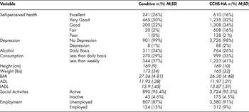
Descriptive statistics (n, M, SD) for health and functional status variables are described in Table 3.
Health and functional status

ADL = activities of daily living; BMI = body mass index; IADL = instrumental activities of daily living.
Self-rated Health, Weight, Height, and BMI
Self-rated health ranged from poor (0% in Candrive II and 4% in CCHS-HA), to excellent (26% in Candrive II and 16% in CCHS-HA). Most participants in both studies evaluated their health as good or very good (72% in Candrive II and 66% in CCHS-HA). Candrive II mean (M = 2, “very good”) falls into the equivalence interval calculated from CCHS-HA data (2.6 ± 1.038) and the TOSTs statistical procedure indicates that the two samples can be deemed equivalent (lower bound t-test = 17.716, p < 0.001; upper bound t-test = –66.46, p < 0.001; see Table 3).
We tested the equivalence of the two samples on height and weight as well as BMI. Mean height of participants in both samples was 168 cm. Candrive II mean for height (M = 168.853 cm) falls into the equivalence interval surrounding the CCHS-HA mean (168.481± 9.572) and the TOSTs procedure yielded significant results (lower bound, t-test = 30.648, p < 0.001; upper bound, t = –31.724, p < 0.001). Candrive II mean for weight (172.593 lbs.) also falls within the boundaries of the interval generated with the CCHS-HA weight average (164.992 ± 31.784) and was found to be statistically comparable (lower bound, t = 35.036; p = 0.0001; upper bound, t = –21.512; p = 0.0001) in both samples. A similar pattern of results was found for the BMI index. BMI average of Candrive II participants (27.36) is within the equivalence interval of the CCHS HA study participants (26.30 ± 4.45) and TOSTS comparisons once again reached significance (lower bound, t = 34.878; p = 0.0001; upper bound, t = –21.476; p < 0.001).
Depression and Alcohol Consumption
Most participants in both samples were not depressed. An estimated 1 per cent of Candrive II participants and 2 per cent of CCHS-HA participants were determined likely to be depressed. The two samples were deemed statistically equivalent (d 2 = .0004, estimated SE of .00018, p < 0.05).
The three categories of alcohol consumption frequency were about equally distributed in both samples (see Table 3) and their distribution is comparable across the two samples (d 2 = .0097 estimated SE = 0037, p < 0.05).
Functional Status
Participants in both studies demonstrated a very high level of functioning on ADL. With the maximum possible score of 12, the CCHS-HA mean was 11.97 (SD = .21) and the Candrive mean 11.93 (SD = .38). The TOSTs procedure confirmed that the two samples were statistically equivalent (lower bound t = 13.599; p < 0.001; upper bound t = –19.961; p < 0.001). Using IADL as the variable of comparison, a similar conclusion is reached. The Candrive II mean (13.904) falls within the CCHS-HA equivalence interval of 13.865 ± .506 and both samples are found to be statistically equivalent (lower bound t = 13.599; p < 0.001; upper bound, t = –19.961; p < 0.001).
Employment and Participation in Social Activities
The analysis performed on the categorical level of employment (d 2 = .0056, estimated SE = 0023, p < 0.05), and social participation (d 2 = .000002, estimated SE = .00003, p < 0.05) allows us to conclude that the Candrive participants were as engaged in social activities as participants from the CCHS-HA study and displayed comparable level of employment.
Frequency of Driving
The last variable examined was self-reported driving frequency. We note that 98 per cent of Candrive II and 80 per cent of CCHS-HA participants drove between 4 and 7 times a week while only 2 per cent of Candrive II and 20 per cent of CCHS-HA participants drove between 1 and 3 times a week. The statistical analysis indicated that the Candrive distribution is not statistically comparable to the CCHS-HA distribution (d 2 = 0.0622, estimated SE = .0035, p > 0.05). Candrive II participants drove significantly more frequently than CCHS-HA participants did.
Discussion
The present findings support the contention that the Candrive II sample of older drivers is representative of the population of older drivers in Canada (derived from the CCHS-HA sample) on the majority of variables that were compared, suggesting that the convenience sample of the Candrive II cohort study population is demographically representative of the larger, older Canadian driver population. The large sample size of the Candrive II study, recruited from multiple sites, with comparison to older drivers from the CCHS-HA (rather than all older adults), likely contributed to the similarities between the samples. Indeed, in both samples, participants were community dwelling and agreed to take part in a research study.
We were able to demonstrate that the Candrive II participants were representative of the Canadian older drivers based on a large and representative sample of older Canadian drivers and on a novel statistical approach to demonstrate equivalence between samples. A major methodological strength of our study is the representativeness and size of the CCHS-HA sample. The sample was statistically designed to provide a valid estimate of the community-dwelling Canadian population in 10 provinces. From that sample, we were able to extract the data of 3,899 drivers over the age of 70. Another strength is that we used an innovative statistical approach to determine whether the Candrive II sample was comparable to the Canadian population of older drivers as estimated through the CCHS-HA study sample. Had we used simple statistical comparisons to demonstrate whether the two samples were different from each other, the chances of finding statistical differences would have been increased simply by virtue of the large sample sizes and the enormous power of Student’s t-test in that context (Cribbie et al., Reference Cribbie, Gruman and Arpin-Cribbie2004). The equivalence testing approach that we used offers a more compelling approach to the question of sample comparability (Cribbie et al., Reference Cribbie, Gruman and Arpin-Cribbie2004). An additional strength of the study is that while many variables were not collected in an identical manner between the two surveys, similar variables were diligently recoded to allow for comparison.
Nevertheless, we found the two samples to differ on certain variables. We noted that a higher proportion of Candrive II participants lived in an urban area and fewer lived in private houses compared with the CCHS-HA sample of drivers, and this was likely due to the geographic location of the Candrive II research sites within seven cities tied to university settings, and the requirement for regular visits of the participants to these assessment sites. In fact, residence in or in proximity (within 50 km of the test site) to these seven cities was a requirement for participation in the Candrive II study (see Marshall et al., Reference Marshall, Man-Son-Hing, Bédard, Charlton, Gagnon and Gélinas2013). Unfortunately, due to small cell sizes, we were unable to stratify the samples according to geographical location. We examined this possibility and concluded that it was statistically inappropriate as it would have reduced the sample size to only a few participants for certain locations (e.g., Thunder Bay, Ontario). Indeed, the CCHS-HA sample is spread out across 10 provinces with some areas having fewer participants. This explains why we observed more Candrive II participants living in urban areas and fewer of them in private residences in comparison to the CCHS-HA participants as a whole. We question the importance of this difference in housing characteristics between the two samples as it is unlikely that housing type alone significantly impacts crash risk.
Another important difference concerns driving frequency. Candrive II participants reported that they drive more frequently than do CCHS-HA study participants. The Candrive II study sample likely over-represents individuals who have an interest in driving over and above those in the general population of drivers the same age. Thus, a limitation of our study is the potential self-selection bias in the Candrive II sample and may explain increased driving frequency among Candrive II participants. This self-selection bias may also relate to participants’ health. In particular, we indicate in the introduction of this article that one of the limitations of convenience sampling, such as the technique used in the Candrive II study, is that drivers who volunteer to participate may be of higher health status in comparison to the general population of older drivers. Although we observed equivalence on the health variables we could compare, we cannot disregard the likelihood that our sample was indeed healthier at the time of recruitment compared to the general population. Had we been able to examine more precise variables, such as those derived through cognitive and/or clinical screening (e.g., blood pressure), instead of relying on self-report measures, we may have observed differences in health.
One key feature of the Candrive study is its longitudinal nature, and while participants’ health was likely better than the average older driver at baseline, it is expected to decline over the course of the study. Data collected over the entire study period will be used to draw conclusions about risks associated with adverse driving outcomes among older drivers.
The variables that we used to determine equivalence between the two samples were selected based solely on whether the variables were statistically comparable. However, there is no certainty that these variables have a direct or indirect effect on driving (e.g., BMI). Admittedly, the CCHA-HA and Candrive II study were developed independently from one another with two very different objectives in mind. Consequently, it is unsurprising that many variables were not statistically comparable due to the way in which they were collected.
The recruitment strategy in the Candrive II study was based principally on community advertising (potential participants contacted the Candrive study, not the opposite) as commonly applied in older drivers’ studies (Emerson et al., Reference Emerson, Johnson, Dawson, Uc, Anderson and Rizzo2012). As a result, the Candrive II research has all that is required to induce self-selection and generate a bias towards a healthy and autonomous sample. The study requires an extensive time commitment from participants with virtually no monetary compensation. Participants’ road behaviors are monitored with an in-car device. Moreover, participants were made aware of the risk of losing their driver’s license as a consequence of new conditions that could affect their driving and may be identified during the study. The fact that only a few differences between the two study samples were noted is remarkable.
Conclusion
In this study, we demonstrated that a large convenience sample of older drivers recruited in the context of the Candrive II longitudinal study was fairly representative of the larger population of Canadian drivers. We observed that on most demographic, health, and functional status variables that we could statistically compare, the convenience sample of older drivers was similar to a much larger representative sample of the population of older drivers, apart from driving frequency, and possibly on health conditions that we could not compare, which are likely explained by the different study designs/purposes.