1 Introduction
Flow separation due to the presence of an adverse pressure gradient, which can be induced by either the prevailing conditions (i.e. flow shear) or the geometrical layout (i.e. flow-path constriction), is a fundamental and widely investigated flow process characterized by a wide range of three-dimensional instabilities. Hence, complex perturbation-sensitive recirculating-flow topologies are common even in the laminar-flow regime and for simplified geometrical configurations (Wilhelm, Härtel & Kleiser Reference Wilhelm, Härtel and Kleiser2003). With reference to high-velocity turbulent liquid flows, the onset of a recirculating-flow pattern having a significant vorticity magnitude is able to cause enough tension at its core so as to force the liquid to nucleate, hence giving rise to a vortical cavity. Vortical cavitation is a flow phenomenon encountered in the natural world (see e.g. Hess Reference Hess2011), as well as in a wide range of engineering applications comprising, among others, ship propellers, turbomachinery blades, high-pressure pumps, fuel injectors and mechanical heart valves (Kini et al. Reference Kini, Bachmann, Fontaine, Deutsch and Tarbell2000). The emergence of cavitation in engineering applications is accompanied by either attractive side effects, i.e. de-agglomeration of particles or deposits and spray atomization, or undesirable side effects, such as noise, vibrations and material erosion.
Depending on the topology of the underlying secondary flow pattern, vortical cavitation can be manifested in the form of either a shed bubble cloud or an elongated vaporous structure. The distinct forms of vortical cavitation that may possibly emerge in various engineering applications have been categorized by Arndt (Reference Arndt2002). The development, temporal evolution and collapse of either one or a combination of the aforementioned forms of vortex cavitation have been extensively investigated by experimental means with reference to shear flows (O’Hern Reference O’Hern1990), as well as two-phase separated flows in clearance passages (Boulon et al. Reference Boulon, Callenaere, Franc and Michel1999), over hydrofoils (Bourgoyne, Ceccio & Dowling Reference Bourgoyne, Ceccio and Dowling2005; Coutier-Delgosha et al. Reference Coutier-Delgosha, Stutz, Vabre and Legoupil2007) and past bluff bodies, e.g. spheres (Brandner et al. Reference Brandner, Walker, Niekamp and Anderson2010). Periodic vortical-cavity shedding in the wake of a hydrofoil has been demonstrated to be enhanced by the vertical velocity fluctuations, which provide the perturbation necessary to trigger a Kelvin–Helmholtz instability responsible for the vortex roll-up (Bourgoyne et al. Reference Bourgoyne, Ceccio and Dowling2005).
A method of specifying the distinct deformation mode of a stationary tip-vortex cavity has been proposed by Pennings et al. (Reference Pennings, Bosschers, Westerweel and van Terwisga2015). The rationale was that the representation in the frequency (Fourier) domain of the high-speed shadowgraphy images obtained should correlate to an analytical formulation describing the dispersion of disturbances in an infinite vortex. Karn, Arndt & Hong (Reference Karn, Arndt and Hong2016) distinguished the favourable closure mechanisms for a supercavity fed with air. Distinct shear-flow instability manifestation processes, comprising, among others, the stable mechanism of the re-entrant jet and combinations of cavitating vortex systems (twin or quad) were identified. With the use of a focused laser, Choi & Ceccio (Reference Choi and Ceccio2007) managed to produce single vapour bubbles located in the core of a three-dimensional longitudinal vortex characterized by a nominal Reynolds number
 $Re=2\times 10^{6}$
. Their experimental investigation comprising high-speed photography and stereo particle image velocimetry (PIV) revealed that the cavity to vortex radius ratio was of the order of 0.1 for varying cavitation numbers, while the cavity was considerably deformed, with length to diameter ratios even exceeding a value of 50. Additional numerical results obtained by Choi et al. (Reference Choi, Hsiao, Chahine and Ceccio2009) for the same flow process demonstrated that for rapid growth of the cavitating bubble the radius oscillates with a frequency that scales with the single-phase vortex time scale
 $\unicode[STIX]{x1D70F}_{V}=2\unicode[STIX]{x03C0}r_{c}/u_{\unicode[STIX]{x1D717},max}$
, where
 $r_{c}$
is the vortex core radius and
 $u_{\unicode[STIX]{x1D717},max}$
is its maximum tangential velocity.
Optical methods have been primarily employed for the visualization of cavitating flows. However, X-ray imaging is currently gaining momentum as a technique suitable to provide insight on the dynamics and composition of three-dimensional cavities. Coutier-Delgosha et al. (Reference Coutier-Delgosha, Stutz, Vabre and Legoupil2007) obtained quantitative data regarding the vapour fraction of the cavity being shed downstream from a wedge-like two-dimensional geometrical constriction. More recently, and referring to a similar geometry, Ganesh, Mäkiharju & Ceccio (Reference Ganesh, Mäkiharju and Ceccio2016) employed X-ray attenuation measurements to elucidate the physical mechanisms governing the cavity shedding behaviour. It was verified that, depending on the cavitation number (
 $CN$
) value, the detachment of coherent vapour clouds is attributed either to the re-entrant jet mechanism or to a shock wave forming in the cavity region due to the adjustment of the local sonic velocity. A number of studies have employed X-ray imaging (attenuation or phase contrast) to visualize highly turbulent two-phase nozzle and spray flows with relevance to the automotive industry and fuel injection equipment (Kastengren et al.
Reference Kastengren, Tilocco, Duke and Powell2012; Im et al.
Reference Im, Cheong, Powell, Lai and Wang2013; Moon Reference Moon2016). For instance, Mitroglou et al. (Reference Mitroglou, Lorenzi, Santini and Gavaises2016) utilized a cone-beam X-ray source and computed tomography to quantify, i.e. provide vapour fraction data for, the time-averaged extent of cavitation in an injector replica orifice. In-nozzle sheet cavitation has been quantified by Duke et al. (Reference Duke, Kastengren, Tilocco, Swantek and Powell2013), who, however, used an interpolation technique to compensate for the small dimensions
 $(5~\unicode[STIX]{x03BC}\text{m}\times 6~\unicode[STIX]{x03BC}\text{m})$
of the monochromatic beam employed. X-ray phase-contrast imaging (XPCI) has, until now, been primarily performed to resolve the velocity field and turbulence level of spray flows produced by real-size fuel injectors (Im et al.
Reference Im, Cheong, Powell, Lai and Wang2013; Moon Reference Moon2016).
The relevant literature survey demonstrates that vortical cavitation has been extensively investigated in unconfined, e.g. tip-vortex, flows, yet there are scarce fundamental studies regarding wall-bounded flows. Also, the referenced studies employing X-ray imaging techniques focus on either sheet/cloud cavitation regimes possibly accompanied by shedding mechanisms or spray flows. The present study offers new experimental data referring to vortical cavitation, as, to the authors’ knowledge, it constitutes the first XPCI investigation to capture in detail the morphological fine features and dynamics of the highly fluctuating elongated coherent cavities arising in an orifice with an abrupt geometrical constriction. The highly transient nature of the nozzle flow, requiring over 60 000 frames per second to be accurately resolved, in conjunction with the fact that the X-rays in the present case must penetrate solid material, pose major visualization difficulties; therefore the high-flux X-rays produced by a synchrotron facility are necessary. The scope of the present study is firstly to demonstrate the suitability of XPCI for the visualization of high-speed two-phase internal flows and, furthermore, to provide estimations on the secondary flow intensity and the level of turbulence within the examined orifice layout for flow conditions ranging from moderate to well-established vortical cavitation.
2 Experimental set-up and post-processing methodology
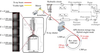
The axisymmetric orifice under investigation was manufactured using a carbon-fibre composite material (TORAYCA TF00S), which causes lower X-ray attenuation compared to metals and, furthermore, provides high structural integrity. The main body of the orifice, depicted in figure 1 along with the main dimensions, produces an asymmetrical flow entering the nozzle hole of diameter equal to 1.5 mm. A metallic needle with a hemispherical tip is inserted into the upstream flow chamber and adjusted to a fixed position. The rationale behind this design concept is to promote flow conditions similar to those prevailing in flow injection equipment. Furthermore, the geometrical layout employed in essence constitutes a flow passage with an abrupt constriction. Contracting geometries, e.g. venturi nozzles (Gopalan & Katz Reference Gopalan and Katz2000; Stutz & Legoupil Reference Stutz and Legoupil2003) or wedge-like flow constrictions (Ganesh et al. Reference Ganesh, Mäkiharju and Ceccio2016), have been widely used to elucidate the fundamentals of cavitating flow. The curved wall upstream of the contraction in the layout of the present investigation promotes the emergence of fluctuating cavitating structures. Details on hydraulic components and instrumentation of the closed flow loop employed to circulate the commercial diesel fuel flowing through the orifice with a steady nominal flow rate have been discussed in detail in Mitroglou et al. (Reference Mitroglou, Stamboliyski, Karathanassis, Nikas and Gavaises2017).
Schematic layout of the experimental set-up (all dimensions are in mm). According to the beam pulsation mode, a single pulse of 150 ps and carrying 16 mA of current is followed, after an interval of
 $1.569~\unicode[STIX]{x03BC}\text{s}$
, by eight short pulses, each one carrying 11 mA, separated by time intervals of 51 ns. Only the bunch of eight pulses was partially utilized in the present investigation (six out of eight).

The XPCI measurements were performed using a white X-ray beam with energy of 6 keV generated by an undulator in the Advanced Photon Source electron storage ring. The attenuated X-ray beam, after its interaction with the injector orifice, impinges on the scintillator crystal, and is converted to visible light (432 nm), subsequently captured by a charge-coupled device (CCD) camera. The beam pulsation mode also depicted in figure 1 allowed a shutter exposure time of 347 ns to be achieved and hence the captured flow can be considered as ‘frozen’. Side-view radiographs at 67 890 frames per second were obtained with a field of view of
 $2.56~\text{mm}\times 2.56~\text{mm}$
discretized by
 $512\times 512~\text{pixels}$
, thus producing a spatial resolution of
 $5~\unicode[STIX]{x03BC}\text{m}~\text{pixel}^{-1}$
. However, it must be noted that the X-ray beam is collimated to a circular cross-section and therefore the overall orifice length had to be segmented into five regions, which were irradiated in a successive manner, i.e. with a time interval between adjacent locations. Moreover, a degree of spatial overlap was maintained between successively irradiated regions, in order to ensure a high signal-to-noise ratio throughout the orifice length.
Similarly to optical techniques, e.g. shadowgraphy or Mie scattering, XPCI takes advantage of the interaction of electromagnetic radiation with matter to produce images with contrast fluctuations. In fact, the attenuation of an X-ray beam can be explicitly correlated to an index of refraction
 $n$
, similar to visible-light physics, yet of complex form,
 $n=\unicode[STIX]{x1D6FF}+\unicode[STIX]{x1D6FD}\text{i}$
, where the real part
 $\unicode[STIX]{x1D6FF}$
corresponds to the phase shift of the X-ray wave and the imaginary part
 $\unicode[STIX]{x1D6FD}$
to the amplitude decrease (absorption) of the wave (Russo Reference Russo2014). Phase-contrast imaging is made possible exactly due to the
 $\unicode[STIX]{x1D6FF}$
value, which is designated by the material composition and the X-ray energy. In essence, the X-ray wave phase shift occurs due to the X-ray (Compton and Rayleigh) scattering through the material mass, which, as emphasized by Wang et al. (Reference Wang, Liu, Im, Lee, Wang, Fezzaa, Hung and Winkelman2008), is orders of magnitude weaker compared to visible light for hydrocarbon fuel. Hence, an X-ray phase-contrast image is primarily designated by strong index gradients, i.e. significant phase alterations, yet, unlike optical methods, information corresponding to each interaction along the beam path is accumulated at the scintillator (Linne Reference Linne2012).
In other words, fine features of the two-phase flow, which usually cannot be captured by conventional optical imaging due to the considerable light scattering in the presence of even negligible vapour content, are highlighted through XPCI. Wang et al. (Reference Wang, Liu, Im, Lee, Wang, Fezzaa, Hung and Winkelman2008) have elucidated the visualization capabilities of both shadowgraphy and XPCI, with reference to spray flows. The failure of shadowgraphy to capture ‘internal’ cavitation features in a nozzle flow has also been pointed out by Mitroglou et al. (Reference Mitroglou, Lorenzi, Santini and Gavaises2016), who observed that a thin cavitation film forming on the curved wall completely prevented the visualization of the morphology of cavitation emerging in the nozzle core.
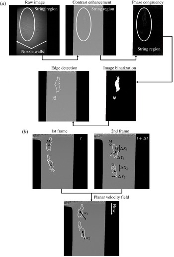
Image post-processing techniques employed: (a) edge detection and (b) derivation of the local velocity field (indicatively for a low-
 $CN$
case). Points
 $M$
and
 $M^{\prime }$
are the centres of mass of the identified vaporous structures at the time instants
 $t$
and
 $\unicode[STIX]{x0394}t$
, respectively;
 $\unicode[STIX]{x0394}t$
corresponds to the time period between consecutive frames, i.e. 0.01473 ms. Flow is from (a) to (b).

Twelve-bit greyscale images were produced by the high-speed camera (Photron FASTCAM SA-Z) used during the investigation, with contrast fluctuation signifying the cavitation extent and form. To prevent overheating of the scintillator, the acquisition of 1000 images was allowed per irradiation event, whereas 16 000 images were obtained in total for each irradiation location to verify the repetitive nature of the flow process. Post-processing treatment of the raw radiographs was required, so as to extract the physical information corresponding to the in-nozzle extent of cavitation and associated dynamic features. Various techniques were employed in a successive manner to detect the edges of the vaporous structures, as depicted in figure 2(a). In order to enhance contrast, the raw radiographs were divided by background images obtained prior to each case examined. The phase congruency method, as described in Kovesi (Reference Kovesi1995), was implemented to recognize the features of interest in the enhanced contrast images. The specific edge-detection methodology surpasses conventional brightness-gradient-based methods, in the sense that salient features in an image are highlighted by the phase and amplitude of the obtained signal in the frequency (Fourier) domain. Hence, phase congruency is not influenced by changes in image brightness or contrast, unlike conventional methods, which analyse the image signal in the spatial domain. Subsequently, the image was binarized by applying a mean filter and proper thresholding, since after phase congruency the cavity interphase appeared much brighter compared to the rest of the image. In a final step, Canny’s algorithm was employed to detect the edges of the identified structure.
Once the morphology of the emerging cavities has been clearly denoted, the planar velocity field can be estimated with the use of a procedure similar to the so-called particle tracking velocimetry (PTV) method, as depicted in figure 2(b). The production of vapour bubbles in cavitating flows is an inherent flow process, and therefore the incorporation of tracer particles, as required for example by the PIV method, is in general avoided since it is possible to modify the two-phase flow topology, especially in the vapour region (Mueller et al. Reference Mueller, Dreyer, Andreini and Avellan2013). Hence, PTV, according to which bubbles (or vaporous structures) are tracked over successive time frames, constitutes a valid and preferred approach (Kitagawa, Hishida & Kodama Reference Kitagawa, Hishida and Kodama2005; Seol et al. Reference Seol, Bhaumik, Bergmann and Socolofsky2007; Sathe et al. Reference Sathe, Thaker, Strand and Joshi2010; Pang & Wei Reference Pang and Wei2013) for the determination of the local velocity field and turbulence intensity (Bröder & Sommerfeld Reference Bröder and Sommerfeld2003; Kitagawa et al. Reference Kitagawa, Hishida and Kodama2005).
The temporally resolved nature of XPCI allows flow fine features to be captured, such as separated bubble clouds (in low-
 $CN$
cases; see e.g. figure 2
b), or interfacial perturbations of distinct shape (in high-
 $CN$
cases). The planar displacement of the centre of mass of identified features along consecutive frames subsequently enables instantaneous measurements of the local velocity field to be made. The traceability of ‘large’ cavities constitutes an issue for conventional PIV/PTV methods (Mueller et al.
Reference Mueller, Dreyer, Andreini and Avellan2013). This is due to the significant light scattering that they induce, leading the CCD camera to saturated brightness levels and intense background noise. The sizes of the structures that have been tracked in the present investigation do not exceed 700
 $\unicode[STIX]{x03BC}\text{m}$
in any of the cases considered. More importantly, the drawback of reduced traceability does not apply for X-ray measurements, since X-ray irradiation interacts only weakly with matter and therefore the cavitating structure interphase can be well captured. For this reason, the use of distinctive flow features in conjunction with XPCI has been extensively employed for velocity (Wang et al.
Reference Wang, Liu, Im, Lee, Wang, Fezzaa, Hung and Winkelman2008; Moon Reference Moon2016) and turbulence (Moon Reference Moon2016) measurements in spray flows. The small exposure time (347 ns) used for the production of radiographs leads to reduced blurriness in the flow fine features, and hence the uncertainty associated with the velocity values and the level of turbulence is low, as reported in § 3.3.
It is essential to point out that the emergence of additional vaporous structures in the orifice, if mistakenly identified as convection of already existing structures, would falsify the velocimetry measurements. Nevertheless, several precautions were taken during the post-processing of the radiographs to prevent such an erroneous practice from occurring, as follows.
-
(i) The projected area of structures identified as possible ‘tracers’ for velocimetry must remain entirely within the irradiated window and within the regions of high signal-to-noise ratios along consecutive frames.
-
(ii) The projected area of ‘tracer’ structures must not differ by more than 10 % between successive frames to minimize the possibility of misidentifying newly emerging structures. In fact, the mean deviation in the projected area of identified structures has been calculated to be approximately equal to 8 %.
-
(iii) The number of structures used to derive the local velocity field must remain the same in two successive frames, i.e. no structures must emerge or collapse in the respective time period.
-
(iv) Structures having a maximum size below
 $700~\unicode[STIX]{x03BC}\text{m}$
were tracked to produce the velocity measurements.

Furthermore, it should be noted that, from the 16 000 images visualized for each location of interest, fewer than 1 % were finally utilized for the velocimetry measurements, thus demonstrating that the imposed filtering is suitable for pinpointing relatively invariant, in terms of size, vaporous structures. However, since cavitation constitutes an inherent flow process influenced by the pressure and velocity fields, the morphology of the structures will inevitably exhibit some variation with time.
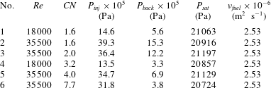
Table 1 summarizes the range of flow conditions considered in the present evaluation. The Reynolds number characterizing the flow was defined as
 $Re=uD/\unicode[STIX]{x1D708}$
, where the nominal velocity
 $u~(=4\dot{V}/\unicode[STIX]{x03C0}D^{2})$
was calculated on the basis of the volumetric flow rate
 $\dot{V}$
and the orifice diameter
 $D~(=1.5~\text{mm})$
. In addition, the cavitation number was defined as
 $CN=(p_{inj}-p_{back})/(p_{back}-p_{sat})$
, where
 $p_{inj}$
,
 $p_{back}$
and
 $p_{sat}$
stand for the upstream (injection), back and saturation pressure, respectively. With regard to the calculation of both non-dimensional quantities, the diesel fuel thermophysical properties required were obtained from the library available in Kolev (Reference Kolev2007). Following a propagation analysis (Moffat Reference Moffat1988) of the experimental errors, the values of
 $Re$
and
 $CN$
are associated with global uncertainties of 3.5 % and 5.0 %, respectively.
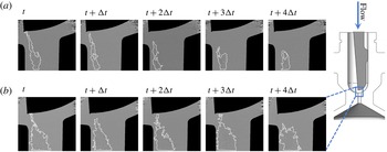
Temporal evolution of the vortical cavitation topology at the nozzle region immediately downstream of the geometrical constriction
 $(Re=35\,500)$
: (a)
 $CN=1.6$
and (b)
 $CN=7.7$
. Here
 $\unicode[STIX]{x0394}t=1.473\times 10^{-5}~\text{s}$
is the time period between consecutive frames.

Experimental test cases investigated. The needle lift is equal to 0.5 mm in all cases.

3 Results and discussion
3.1 Morphology and dynamical behaviour of the vortical structures
A sequence of post-processed radiographs of the flow region in the vicinity of the flow constriction, as depicted in figure 3, demonstrates that cavitation manifestation occurs in the form of elongated cavities. As also discussed in § 2, the radiography images presented in figure 3 constitute planar projections of the cavity in each case, yet produced by strong gradients of the refractive index and thus highlight the most profound features. Referring to
 $CN=1.6$
(figure 3
a), where the flow is moderately cavitating, a slender vaporous structure sets in, with a highly varying morphology owing to the conflicting viscous and surface-tension effects. Increase of the cavitation number to a value of
 $CN=7.7$
(figure 3
b) causes the cavity to grow in size and exhibit a relatively smoother topology with an invariant core. Referring to both figures 3(a) and 3(b), the horizontal white lines closing the interfaces at the lower side of the panels actually signify the extent of the control window for which high signal-to-noise ratio could be obtained at each location.
A distinct feature that is common for the two cases depicted is that the cavity, although located closer to the left-hand side wall due to the flow asymmetry, is not attached to it. Hence, its formation cannot be attributed to a flow separation occurring downstream of the constriction, a common feature of abruptly contracting flows (Lanzerstorfer & Kuhlmann Reference Lanzerstorfer and Kuhlmann2012). On the contrary, the onset of the cavity is attributed to a three-dimensional flow separation occurring upstream of the constriction due to the adverse pressure gradient in the region. The secondary swirling flow motion is subsequently being convected downstream by the main flow, thus giving rise to a longitudinal vortex. Besides, the wall curvature is expected to promote vortical motion through the well-known Goertler instability (Bottaro Reference Bottaro1993). As illustrated by the first time instant of figure 3(a,b), the vapour tube tends to attach to the needle tip; this constitutes proof that the underlying cause is indeed a longitudinal vortex, as, according to the second Helmholtz theorem, a vortex filament must extend to a boundary or form a closed loop (Batchelor Reference Batchelor1967). The strong centrifugal forces prevailing at the vortex core cause the liquid to cavitate. Especially referring to
 $CN=7.7$
, the well-defined interface and the invariant core of the cavity constitute strong indications of a cavity filled with pure vapour occupying the entire nozzle length.
Since the cavitation regime examined is manifested in the form of coherent elongated vaporous structures of significant size, the beam interactions with interfaces along its path are limited and therefore the emerging cavities can be properly resolved. In the case of cloud cavitation, it would be possible to track only the outer edges of the cavitation extent and not the individual interface of each single bubble. Especially for the high-
 $CN$
cases (
 $CN\geqslant 3.2$
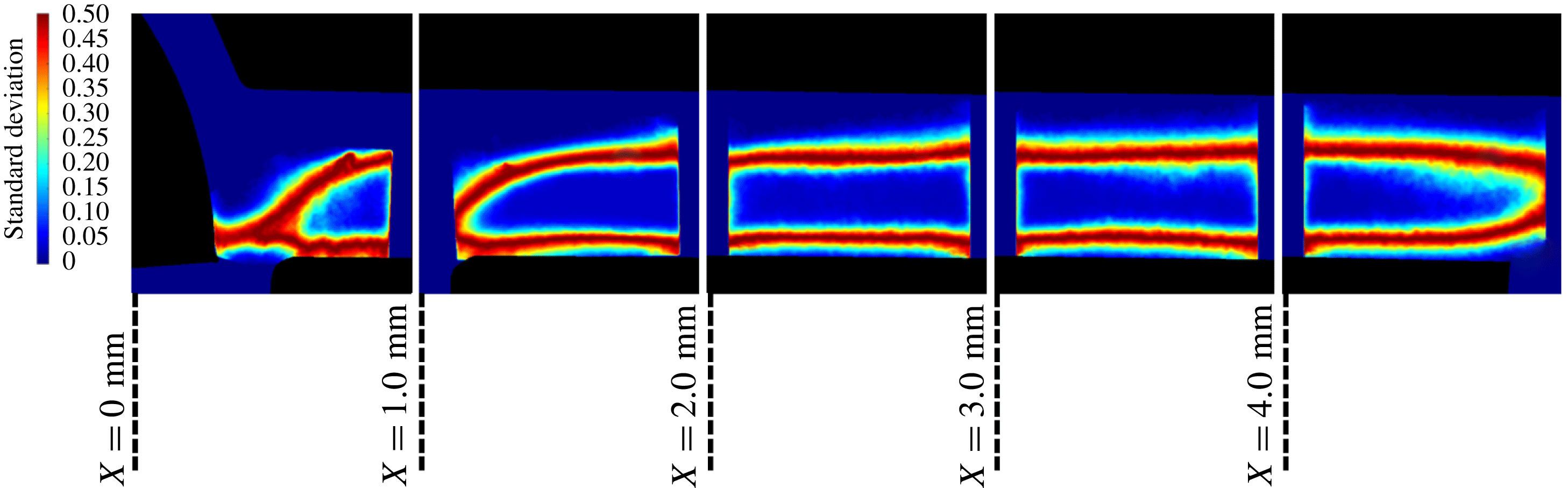
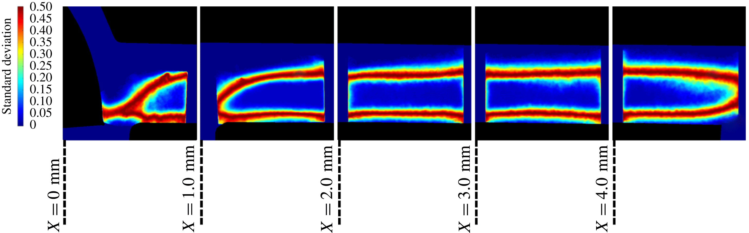
) used for the derivation of the secondary flow intensity and turbulence level, as will be discussed in the following sections, the standard deviation images derived using all the radiographs obtained at each location further demonstrate that no fluctuations occur in the cavity core, yet high standard deviation is evident at localized regions, signifying intense interfacial perturbations, as shown in figure 4. Standard deviation refers to the brightness variation of each pixel against its average value and, in essence, is explicitly correlated to the flow dynamic behaviour. In other words, a low standard deviation signifies that the pixel brightness remains relatively invariant and hence vapour is either absent or present. On the contrary, high standard deviation is indicative of a fluctuating behaviour with reference to vapour formation and collapse. It constitutes a quantity suitable for the identification of transient cavitating structures, as also demonstrated by Mitroglou et al. (Reference Mitroglou, Lorenzi, Santini and Gavaises2016).
Hence, liquid–vapour interfaces are met by the beam only in two distinct locations for the most part of the orifice, signifying that the extensive vapour content evident in figure 3(b) corresponds to a single structure and not to obscured clouds of bubbles. It has also been demonstrated by the various studies in the literature referring to tip-vortex cavitation that vortical cavitation is manifested in the form of a single elongated cavity of significant extent and not as a large cloud of indiscernible bubbles. For instance, in the work of Pennings et al. (Reference Pennings, Bosschers, Westerweel and van Terwisga2015), vortical cavitation is clearly manifested in the form of a single cavity, although the Reynolds number is higher, i.e. the level of turbulence is increased, compared to the present investigation. However, the cavitation number in that case is lower than
 $CN=4.0$
(based on the definition employed in this study), i.e. the cavitation regime is less established.
For the cases corresponding to moderately cavitating flow (
 $CN=1.6$
–
 $2.0$
), the topology of vapour structures exhibits a significant degree of variation, especially in the flow region in the vicinity of the constriction
 $(X\leqslant 2~\text{mm})$
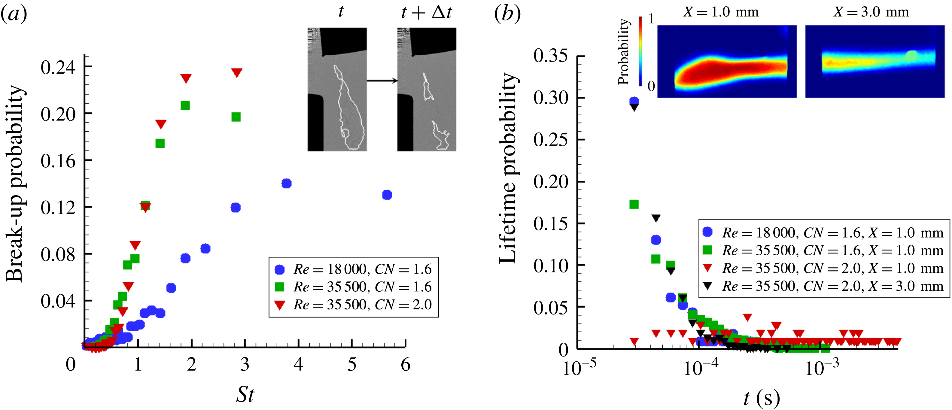
. Figure 5 illustrates the effect of the prevailing flow conditions on the periodicity of the manifested flow phenomena. More specifically, figure 5(a) depicts the break-up probability of a coherent elongated structure into two (or more). To ensure a straightforward comparison between the different cases examined, the break-up probability is presented in correlation to the Strouhal number
 $St=fL/U$
,
 $f$
being the phenomenon manifestation frequency,
 $L~(=5~\text{mm})$
the nozzle length and
 $U$
the nominal flow velocity.
Standard deviation image produced by 16 000 radiographs for each location (
 $Re=35\,500$
,
 $CN=4.0$
). The extensive regions of low standard deviation (blue colour) demonstrate that a stable elongated cavity arises in the orifice with distinct interfacial perturbations (evident as red stripes at the upper and lower extremities of the structure for
 $1.0~\text{mm}\leqslant X\leqslant 4.0~\text{mm}$
. Flow is from left to right.
Cavity break-up probability and lifetime: (a) effect of the flow conditions on the cavity break-up behaviour
 $(X=0.0~\text{mm})$
and (b) cavity lifetime probability for different flow conditions and locations along the channel length. The average cavity image for
 $Re=35\,500$
and
 $CN=2.0$
is depicted as an inset illustrating its fluctuating topology at the closure region
 $(X=3.0)$
. A small artefact is also evident. The maximum experimental uncertainty is equal to 3.7 % and 1.7 % referring to the
 $St$
and lifetime values, respectively.

As
 $Re$
and
 $CN$
increase, the break-up frequency decreases, i.e. the structures gain in coherence, while the periodicity of the phenomenon is also enhanced as the prevailing
 $St$
number values obtain higher probability values. Additionally, as elucidated by figure 5(b), depicting the cavity lifetime probability, increase of
 $Re$
and
 $CN$
causes the vortex cavities to live longer. The cavity lifetime is, in essence, indicative of the periodicity of cavity collapse; since it has been verified that cavitation sets in due to vortex flow motion, its collapse should be attributed to the loss of coherence of the underlying vortex. For
 $Re=18\,000$
and
 $CN=1.6$
, the maximum string life is, in essence, equal to 0.1 ms. It must be pointed that there is a 0.3 probability for the cavity life to be even lower than the minimum lifetime that can be visualized by the method employed. As the Reynolds number increases to 35 500, while the
 $CN$
is maintained constant, the distribution of possible lifetimes is shifted towards larger values approximately up to 0.3 ms. Yet once again approximately 30 % of the vortical cavities recorded have a lifetime smaller than 0.03 ms. Increase of the
 $CN$
value to 2.0 has a considerable effect on string stability, since the probability distribution becomes more even across the range 0.02–0.2 ms.
The effect of the flow conditions on the cavity lifetime is justifiable since increase of the Reynolds number, i.e. of the mean flow velocity, enhances the secondary flow vorticity magnitude, which is responsible for the string formation. Furthermore, increase of the
 $CN$
number, i.e. decrease of the back pressure, leads to a pressure distribution in the nozzle closer to the cavitation threshold and thus a more coherent cavity is established. Figure 5(b) also indicates that the cavity coherence does not decay simultaneously along the orifice length. The cavity exhibits a long lifetime at the location close to the needle tip
 $(X=1.0~\text{mm})$
while, on the contrary, at a location further downstream
 $(X=3.0~\text{mm})$
its lifetime is much shorter and is indicative of a flapping behaviour at the cavity closure region (refer to the inset of figure 5
b).
3.2 Estimation of the vortical motion magnitude
The nucleation of a cavity within a vortex core causes the radial displacement of liquid towards the vortex outer region. The large tension required for cavity inception has been demonstrated to lead to an abrupt growth of its radius, which reaches a maximum value due to the increasing radial pressure and subsequently oscillates around that value with a period that scales with the vortex time scale (Choi et al. Reference Choi, Hsiao, Chahine and Ceccio2009). Hence, in order to obtain an indication of the magnitude of the underlying vortical flow field, the temporal evolution of the cavity radius was measured in a region close to its onset. Further downstream, viscous damping effects come into play, as the cavities slightly increase in size; yet the underlying vortices have possibly lost their coherence (O’Hern Reference O’Hern1990).
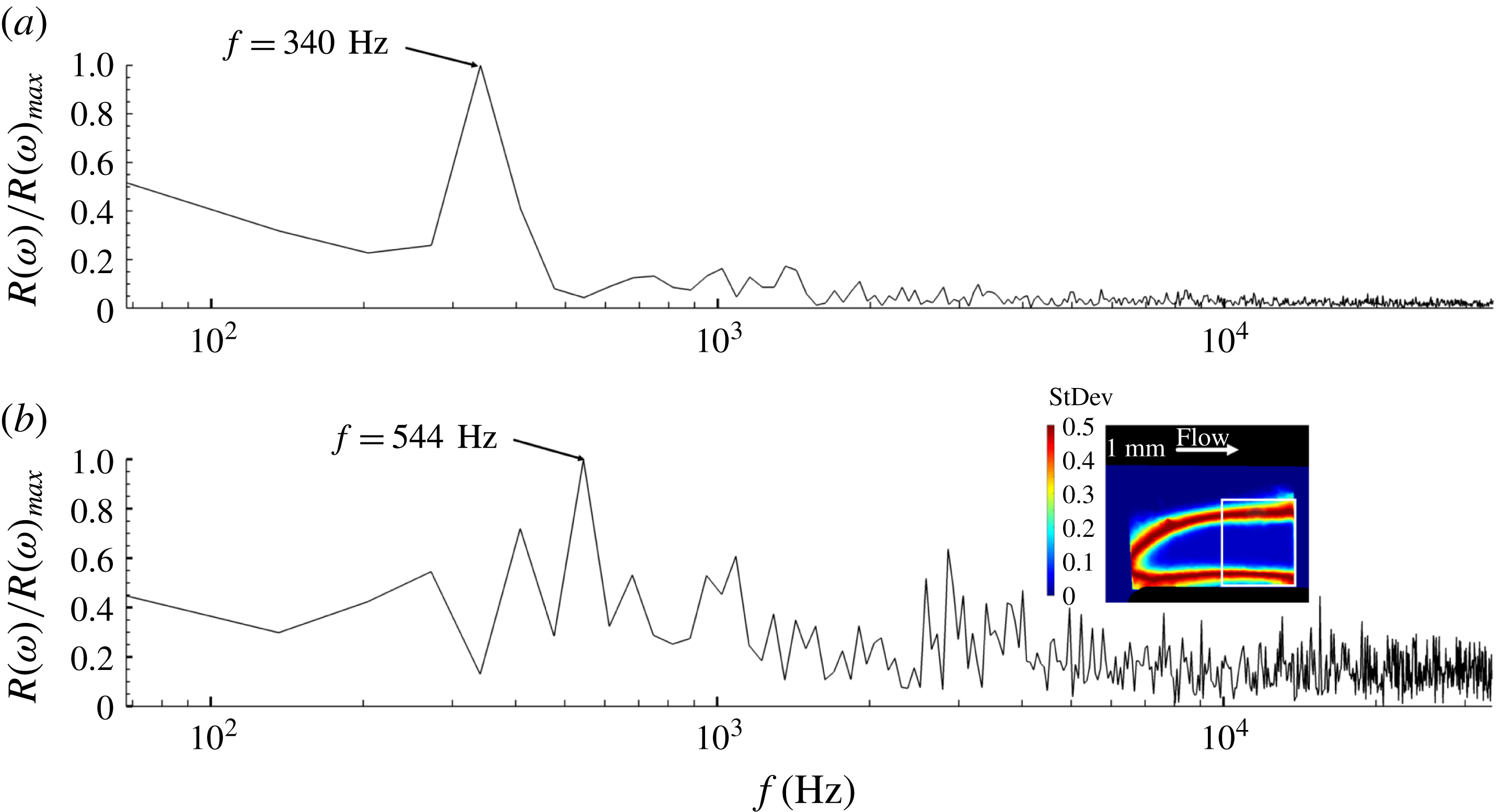
Fourier analysis of the radius waveform for two cases characterized by similar
 $CN$
, yet different Reynolds number values, revealed the existence of different prevailing oscillation frequencies, as depicted in figure 6. The oscillation of the coherent vortical cavities for high cavitation numbers
 $(CN>3.0)$
could be attributed to the fluctuating pressure field beyond the cavity edge. This would have an effect on the recorded time evolution of the cavity radius and thus on the frequency spectrum depicted on figure 6, which is correlated to the underlying vortex intensity. It must be noted that the specific cases have been selected, as the cavities have been verified, through averaging of the radiographs, to exhibit steady cores approximately throughout the entire length of the orifice. The spectral peaks corresponding to the prevailing frequencies have also been verified to remain invariant for the different sets of radiographs obtained (1000 frames each). By comparing figures 6(a) and 6(b), it is evident that the twofold increase of
 $Re$
from 18 000 to 35 500 shifts the prevailing frequency to a higher value, 544 instead of 340 Hz. The cavity radius has been measured to increase from 0.306 to 0.388 mm. Taking into account that the recirculation intensity
 $\unicode[STIX]{x1D6E4}$
scales directly with the fluctuation frequency
 $f$
, i.e.
 $\unicode[STIX]{x1D6E4}\sim f4\unicode[STIX]{x03C0}^{2}r_{c}^{2}$
, assuming that the cavity (refer to the inset of figure 6
b) to vortex core radii (
 $r_{b}/r_{c}$
) ratio remains constant, as proposed for example by Arndt & Keller (Reference Arndt and Keller1992), the intensity ratio
 $\unicode[STIX]{x1D6E4}_{CN=4.0,Re=35\,500}/\unicode[STIX]{x1D6E4}_{CN=3.2,Re=18\,000}$
is equal to 2.57.
Frequency spectrum of the average cavity radius
 $r_{b}$
waveform: (a)
 $Re=18\,000$
,
 $CN=3.2$
and (b)
 $Re=35\,500$
,
 $CN=4.0$
. The radius has been averaged along a control window (white square area) shown in conjunction with a contour plot of the image standard deviation in the inset of panel (b).

A number of theoretical models have been proposed in the literature for the prediction of the tangential velocity distribution along the span of a two-dimensional vortex. The well-known Rankine, Gaussian and Lamb–Oseen vortex models (Arndt Reference Arndt2002; Choi et al. Reference Choi, Hsiao, Chahine and Ceccio2009; Pennings et al. Reference Pennings, Bosschers, Westerweel and van Terwisga2015) can be considered to calculate the recirculation intensity exactly at the moment of vortical cavitation inception as follows:
 $$\begin{eqnarray}\displaystyle & \displaystyle \frac{p_{c}-p_{o}}{\unicode[STIX]{x1D70C}}=-\unicode[STIX]{x1D702}\left(\frac{\unicode[STIX]{x1D6E4}}{2\unicode[STIX]{x03C0}r_{c}}\right)^{2},\quad \unicode[STIX]{x1D702}=1\text{ (Rankine vortex) or }\unicode[STIX]{x1D702}=0.87\text{ (Gaussian vortex)}, & \displaystyle \nonumber\\ \displaystyle & & \displaystyle\end{eqnarray}$$
 $$\begin{eqnarray}\displaystyle & \displaystyle \frac{p_{c}-p_{o}}{\displaystyle \frac{1}{2}\unicode[STIX]{x1D70C}\left(\frac{\unicode[STIX]{x1D6E4}}{2\unicode[STIX]{x03C0}r_{c}}\right)^{2}}=-C_{p,min},\quad C_{p,min}=-1.74\text{ (Lamb–Oseen vortex)}, & \displaystyle\end{eqnarray}$$
where
 $p_{c}$
and
 $p_{o}$
are the pressures at the vortex core and far field, respectively, with the latter being assigned the value of the outlet pressure for the production of results presented below. Recently, Pennings et al. (Reference Pennings, Bosschers, Westerweel and van Terwisga2015) considered the following theoretical correlation between the size of a cavitating vortex and pressure:
 $$\begin{eqnarray}\frac{p_{c}-p_{o}}{\unicode[STIX]{x1D70C}}=-\frac{1}{2}\unicode[STIX]{x1D70C}\left(\frac{\unicode[STIX]{x1D6E4}}{2\unicode[STIX]{x03C0}}\right)^{2}\frac{1}{r_{b}^{2}+r_{c}^{2}},\end{eqnarray}$$
where
 $r_{b}$
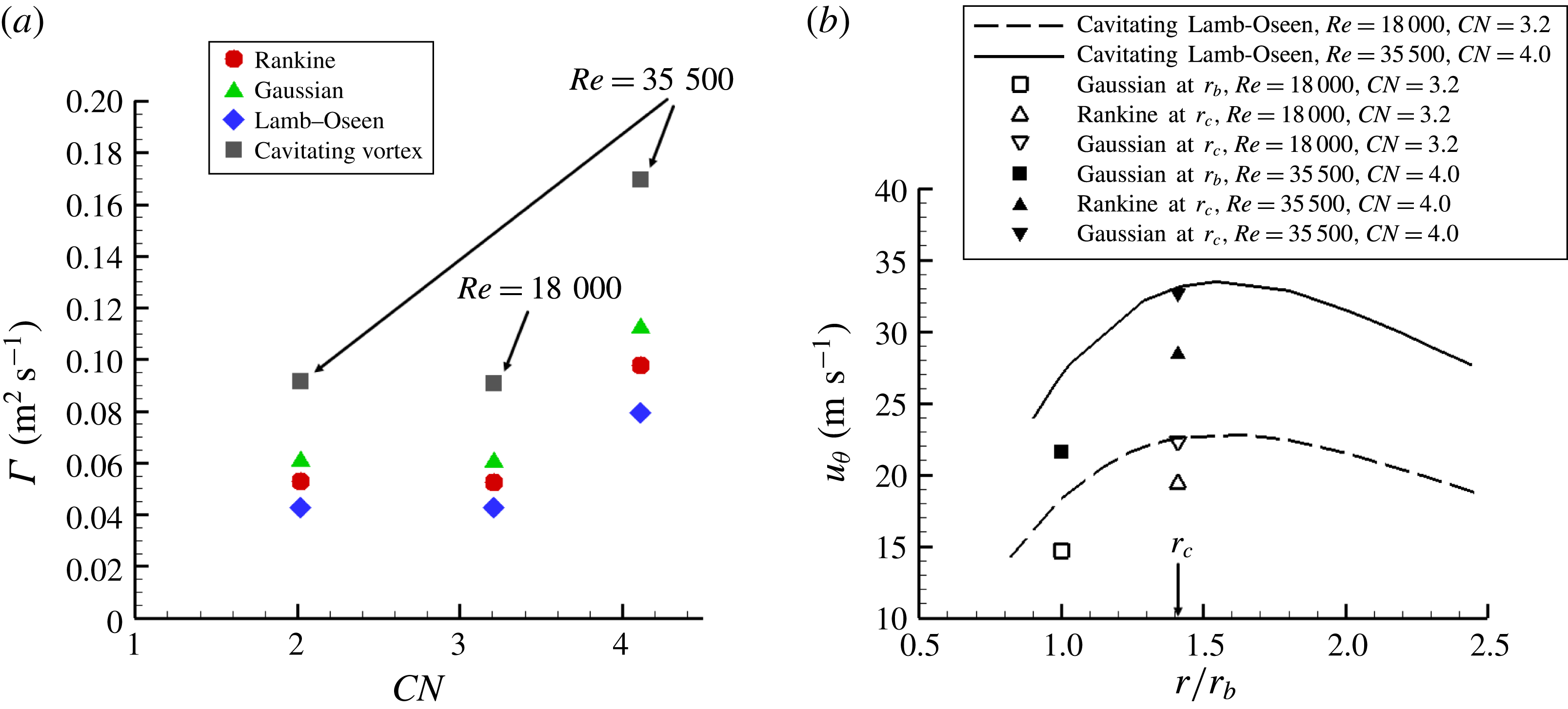
is the cavity (bubble) radius. It is essential to note that such models, however, do not account for three-dimensional or flow confinement effects and have been primarily employed for the prediction of tip cavitating vortices. Nevertheless, (3.1)–(3.3) will be employed in this study to provide an initial estimation of the secondary flow magnitude within the orifice. Figure 7(a) depicts the vortex intensity calculated for the cases where a coherent vortical cavity was detected, considering the measured values of the outlet pressure
 $p_{o}$
and cavity (bubble) radius
 $r_{b}$
and assuming that the pressure at the vortex axis is adjusted to the saturation pressure due to the onset of the cavity. The case corresponding to
 $Re=35\,500$
,
 $CN=7.7$
has not been considered for the analysis, as it was verified that, despite the increase of
 $CN$
, the cavity extent remained invariant, an indication of the increased influence of geometry confinement on the vortical flow.
In general,
 $\unicode[STIX]{x1D6E4}$
values calculated using the cavitating vortex correlation (3.3) are higher compared to the respective predictions (3.1)–(3.2) for single-phase flow, which is in agreement with the well-established conclusion that the presence of cavitation enhances the magnitude of vortical motion (Koukouvinis et al.
Reference Koukouvinis, Mitroglou, Gavaises, Lorenzi and Santini2017). It is interesting to note that
 $\unicode[STIX]{x1D6E4}\approx 0.09~\text{m}^{2}~\text{s}^{-1}$
for both cases characterized by
 $(Re,~CN)=(18\,000,~3.2)$
and (35 500, 4.0), a trend indicative of the combined effect of flow velocity and cavitation on the secondary flow pattern. Once again, considering (3.3) for a cavitating vortex, the ratio
 $\unicode[STIX]{x1D6E4}_{CN=4.0,Re=35\,500}/\unicode[STIX]{x1D6E4}_{CN=3.2,Re=18\,000}$
is equal to 1.86, which compares well, considering the model limitations already mentioned, with the respective value 2.57 produced by the frequency analysis (refer to figure 4). The agreement between the two approaches constitutes evidence that the theoretical model reported by Pennings et al. (Reference Pennings, Bosschers, Westerweel and van Terwisga2015) offers acceptable accuracy for the prediction of the secondary flow tangential velocity.
(a) Vortex flow magnitude
 $\unicode[STIX]{x1D6E4}$
as predicted by the various theoretical models based on the experimental data. Since data on the core radius of the single-phase vortex are not available, an approximation based on the theoretical conclusion of Arndt & Keller (Reference Arndt and Keller1992) is made to correlate the measured vaporous tube
 $r_{b}$
to the vortex core radius
 $r_{c}$
based on the conservation of angular momentum, i.e.
 $r_{b}=0.71r_{c}$
. The core radius
 $r_{c}$
is the distance to the vortex axis where the tangential velocity is maximum. The experimental uncertainty for
 $\unicode[STIX]{x1D6E4}$
lies in the range 2.2 %–3.0 %. (b) Comparison of tangential velocity values as predicted using (3.4) (symbols) and (3.5) (lines), along with the azimuthal velocity predictions
 $u_{\unicode[STIX]{x1D717}}(r)=\unicode[STIX]{x1D6E4}/2\unicode[STIX]{x03C0}r$
for a theoretical Rankine vortex. The experimental uncertainty for
 $u_{\unicode[STIX]{x1D717}}$
is of the order of 2.4 %–3.8 %.

Based on the calculated recirculation intensity
 $\unicode[STIX]{x1D6E4}$
for a single-phase vortex (3.1), the tangential (azimuthal) velocity can be determined, for instance, if a Gaussian profile is assumed, as in Choi & Ceccio (Reference Choi and Ceccio2007):
 $$\begin{eqnarray}u_{\unicode[STIX]{x1D703}}(r)=\left(\frac{\unicode[STIX]{x1D6E4}}{2\unicode[STIX]{x03C0}r}\right)\left[1-\exp \left(-a\left(\frac{r}{r_{c}}\right)^{2}\right)\right],\quad (\text{Gaussian vortex}),\end{eqnarray}$$
where
 $\unicode[STIX]{x1D6E4}$
is calculated according to (3.1) and
 $a=1.255$
. However, for a cavitating vortex of a viscous fluid, the azimuthal velocity in the region of the interface obtains a different behaviour compared to a non-cavitating vortex (Pennings et al.
Reference Pennings, Bosschers, Westerweel and van Terwisga2015):
 $$\begin{eqnarray}\left.\begin{array}{@{}c@{}}\displaystyle u_{\unicode[STIX]{x1D703}}(r)=\left(\frac{\unicode[STIX]{x1D6E4}}{2\unicode[STIX]{x03C0}r}\right)\left[1-\unicode[STIX]{x1D6FD}\exp \left(-a\left(\frac{r}{r_{c}}\right)^{2}\right)\right],\\ \displaystyle \unicode[STIX]{x1D6FD}=\frac{r_{c}^{2}}{r_{c}^{2}+\unicode[STIX]{x1D701}r_{b}^{2}}\quad \text{(cavitating Lamb–Oseen vortex)},\end{array}\right\}\end{eqnarray}$$
where
 $\unicode[STIX]{x1D6E4}$
is calculated according to (3.1) and
 $\unicode[STIX]{x1D701}=1.2564$
. Equation (3.5) predicts the azimuthal velocity profile for a cavitating Lamb–Oseen vortex and has been plotted, based on the experimental data, in figure 7(b) for two examined cases, characterized by different
 $Re$
and
 $CN$
values. The respective velocity values based on the Gaussian and Rankine vortex theoretical models have also been plotted at locations corresponding to the cavity interface (
 $r/r_{b}=1$
) and the radius of the viscous core. As is evident, the single-phase Rankine vortex model predicts lower velocities in both regions of interest, whereas the Gaussian profile, although in agreement with the prediction of (3.5) referring to the azimuthal velocity at
 $r_{c}$
, leads to underprediction of the respective velocity at the bubble radius in both cases. Hence, the remarks of Pennings et al. (Reference Pennings, Bosschers, Westerweel and van Terwisga2015) on the modified vorticity due to the presence of an elongated cavity and the findings of Koukouvinis et al. (Reference Koukouvinis, Mitroglou, Gavaises, Lorenzi and Santini2017) demonstrating that increase of
 $CN$
in a similar nozzle flow increased the magnitude of tangential velocity are in agreement with the results shown in figure 7(b).
3.3 Velocity field and level of turbulence
The local velocity field was measured at the nozzle regions where the cavity topology exhibits high standard deviation. Nevertheless, only structures below
 $700~\unicode[STIX]{x03BC}\text{m}$
were tracked in these regions, in accordance with the methodology reported in § 2. The average measured velocity along the channel length compares well with the nominal velocity based on the imposed flow rate, with the deviation being equal to 6.4 % and 6.7 % for the cases corresponding to
 $Re=18\,000$
and
 $Re=35\,500$
, respectively. Since a considerable number of point velocity values were measured at the lower cavity region, the calculation of local velocity fluctuations, indicative of the level of turbulence along the nozzle length, was made possible.
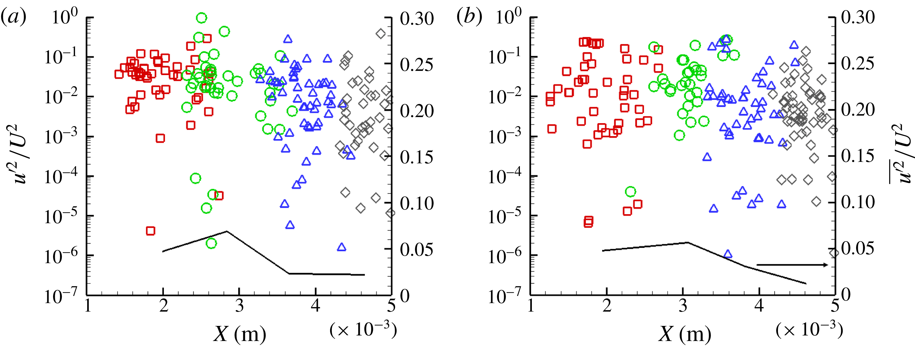
Axial velocity fluctuations at
 $Y\approx 0.620\pm 0.04~\text{mm}$
for (a)
 $Re=18\,000,~CN=3.2$
and (b)
 $Re=35\,500,~CN=7.7$
: ▫,
 $X=1.0~\text{mm}$
; ○,
 $X=2.0~\text{mm}$
; ▵,
 $X=3.0~\text{mm}$
; ♢,
 $X=4.0~\text{mm}$
. The black line corresponds to the averaged quantity per irradiation location. The experimental uncertainty associated with
 $u^{\prime 2}/U^{2}$
lies in the range 6.6 %–7.1 %, whereas the experimental uncertainty in the axial location values is equal to 2.5 %.

Figure 8(a,b) depicts the axial-velocity fluctuation constituent
 $u^{\prime }$
in non-dimensional form. A comparison between the two panels reveals that turbulence is suppressed as
 $CN$
increases, since figure 8(a) exhibits slightly higher fluctuation values, although it corresponds to
 $Re=18\,000$
, along the orifice length, compared to figure 8(b), corresponding to
 $Re=35\,500$
. These findings are in agreement with the numerical results of Koukouvinis et al. (Reference Koukouvinis, Mitroglou, Gavaises, Lorenzi and Santini2017) for a similar orifice layout. Also, the distribution of the averaged quantity seems to follow a similar trend to that reported in Koukouvinis et al. (Reference Koukouvinis, Mitroglou, Gavaises, Lorenzi and Santini2017), i.e. reaching a maximum value and decreasing as the orifice outlet is approached, with the exception of regions of bubble collapse. The increased turbulence at the channel outlet (
 $X\geqslant 4$
) detected for
 $Re=18\,000$
and
 $CN=3.2$
is exactly attributed to the cavity partial collapse close to the orifice outlet, which perturbs the local velocity field. For
 $CN=7.7$
the string retains a stable core even at the orifice outlet.
4 Conclusions
The present study has demonstrated the applicability of temporally resolved XPCI for the elucidation of transient vortical cavitation arising in a highly turbulent nozzle flow. X-rays penetrating material have been demonstrated to produce enough phase contrast to capture fine features of in-nozzle cavitation in a time-resolved manner. To the authors’ knowledge, relevant studies illustrating the morphology and dynamics of highly fluctuating vaporous structures emerging in internal flows in such detail are currently not available in the literature. Post-processing of a large number of side-view radiographs revealed that, in geometrical layouts with an abrupt contraction, where wall curvature also affects the flow, vortex cavitation is promoted over cloud cavitation and that the dynamical behaviour of the arising cavity is highly influenced by the prevailing flow conditions (
 $Re$
and
 $CN$
).
A methodology suitable for the derivation of the underlying flow intrinsic features, i.e. secondary flow intensity and turbulence level, has been presented. Frequency analysis of the measured cavity radius allowed estimations to be made on the recirculation intensity for different cases, and the intensity
 $\unicode[STIX]{x1D6E4}$
results were found to be in agreement with the predictions of a cavitating vortex theoretical model reported by Pennings et al. (Reference Pennings, Bosschers, Westerweel and van Terwisga2015). Based on the calculated vorticity magnitude
 $\unicode[STIX]{x1D6E4}$
, the distribution of azimuthal velocity along the vortex span was calculated and it was verified that increased values are obtained at a location corresponding to the cavity interface compared to single-flow vortices. Furthermore, measurements of the flow turbulence level not currently available in the literature for the present geometrical configuration and cavitation regime have also been obtained. It has been demonstrated that it is possible to estimate the local velocity field by tracking the vaporous structures in an experimental approach similar to particle tracking velocimetry. The measured velocity fluctuations along the orifice length verified the findings of Koukouvinis et al. (Reference Koukouvinis, Mitroglou, Gavaises, Lorenzi and Santini2017) demonstrating that turbulence is suppressed in the presence of well-established cavitation.
Acknowledgements
The research leading to these results has received funding from the MSCA-ITN-ETN of EU H2020 programme, under REA grant agreement no. 642536. The authors would also like to acknowledge the contribution of The Lloyd’s Register Foundation. The Lloyd’s Register Foundation helps to protect life and property by supporting engineering-related education, public engagement and the application of research. This research used resources of the Advanced Photon Source, an Office of Science User Facility operated for the US Department of Energy (DOE) by Argonne National Laboratory under Contract No. 53697. The assistance of Mr M. Lorenzi during the experimental investigation is gratefully acknowledged.