

Introduction
Since the 1980s, a steady flow of discoveries of Mesozoic fossils worldwide has transformed our understanding of the earliest phases of the avian evolution (e.g., Sanz et al. Reference Sanz, Bonaparte and Lacasa1988, Reference Sanz, Chiappe and Buscalioni1995, Reference Sanz, Chiappe, Pérez-Moreno, Buscalioni, Moratalla, Ortega and Poyato-Ariza1996; Chiappe and Calvo Reference Chiappe and Calvo1994; Hou Reference Hou1997; Clarke and Norell 2002; Zhou and Zhang Reference Zhou and Zhang2002; Zhou et al. Reference Zhou, Chiappe and Zhang2005, Reference Zhou, Zhang and Li2009; Chiappe Reference Chiappe2007; Zhang et al. Reference Zhang, Zhou and Benton2008; O’Connor et al. Reference O’Connor, Gao and Chiappe2010; Brusatte et al. Reference Brusatte, O’Connor and Jarvis2015). Numerous extinct lineages have been recorded—particularly from the Early Cretaceous of northeastern China (Chiappe and Meng Reference Chiappe and Meng2016)—and their evolutionary relationships and ecological differentiation have been deciphered (e.g., Chiappe et al. Reference Chiappe, Ji, Ji and Norell1999, Reference Chiappe, Zhao, O’Connor, Chunling, Wang, Habib and Cheng2014; Chiappe and Witmer Reference Chiappe and Witmer2002; You et al. Reference You, Lamanna, Harris, Chiappe, O’Connor, Ji, Jun-chang, Chong-xi, Da-qing, Xing, Lacovara, Dodson and Ji2006; Bell and Chiappe Reference Bell and Chiappe2011; O’Connor et al. Reference O’Connor, Chiappe and Bell2011). Nonetheless, important questions about the aerodynamic competence of these early relatives of modern birds have remained poorly answered. This is largely due to our inability to characterize in these extinct birds a series of key variables known to influence the flight of their living counterparts. Wings are the anatomical structures that allow birds to travel through the air (their aerodynamic design generates lift force necessary to support the animal’s weight, allowing the bird to focus its muscles’ work on flapping the wings to overcome aerodynamic drag; Pennycuick Reference Pennycuick2008). From an aerodynamic point of view, bird wings can be characterized by two basic measurements, wingspan (B) and wing area (S L), defined as the distance from one wing tip to the other and the area that supports the bird’s airborne flight, respectively.
To study the aerial behavior of the stem birds, some authors have obtained values for B and S L from outline reconstructions based on well-preserved specimens such as Archaeopteryx (Yalden Reference Yalden1971, Reference Yalden1984; Elzanowski Reference Elzanowski2002; Longrich Reference Longrich2006; Wellnhofer Reference Wellnhofer2008) and Hongshanornis (Chiappe et al. Reference Chiappe, Zhao, O’Connor, Chunling, Wang, Habib and Cheng2014). However, these types of studies are scarce and can only be confidently applied to nearly complete avian fossils with well-preserved flight feathers. An alternative to body reconstruction is to derive allometric equations adjusted in extant birds to estimate B and S L in extinct birds that preserve the variable(s) included in the equations. Scaling equations of B and S L on body mass (BM) have been obtained from modern data sets (e.g., Greenwalt Reference Greenwalt1975; Viscor and Fuster Reference Viscor and Fuster1987; Pennycuick Reference Pennycuick2008; Tennekes Reference Tennekes2009), and in some cases they have been applied to fossil stem birds (e.g., Sanz et al. Reference Sanz, Álvarez, Soriano, Hernández-Carrasquilla, Pérez-Moreno and Meseguer2002). However, given that the BM of any extinct bird is also an estimated value, which can be subject to different errors and biases (see following paragraph), the allometric equations for B and S L should be derived from morphological traits that are preserved in the fossils studied (e.g., measurements of their bones and feathers).
As recently discussed by Serrano et al. (Reference Serrano, Palmqvist and Sanz2015), any estimated parameter derived from regression functions can be affected by sources of error from statistical, phylogenetic, ecological, and taphonomic nature. Namely, these biases may arise from limitations imposed by: (1) sampling availability and differences in taxonomic diversity (see Mendoza et al. Reference Mendoza, Janis and Palmqvist2006; De Esteban-Trivigno et al. Reference De Esteban-Trivigno, Mendoza and De Renzi2008), (2) multicollinearity (see Mitchell-Olds and Shaw Reference Mitchell-Olds and Shaw1987; Bowerman and O’Connell Reference Bowerman and O’Connell1990; Quinn and Keough Reference Quinn and Keough2001), (3) statistical nonindependence of species given their historical relationships (see Felsenstein Reference Felsenstein1985; Harvey and Pagel Reference Harvey and Pagel1991), (4) uncertainty on the adequacy of assuming similar scaling patterns for crown and stem taxa (see Carrano Reference Carrano2001; Smith Reference Smith2002; Packard et al. Reference Packard, Boardman and Birchard2009; Campione and Evans Reference Campione and Evans2012; Field et al. Reference Field, Lynner, Brown and Darroch2013), (5) effects of the functional adaptations on the morphology of wing bones (see Cubo and Casinos Reference Cubo and Casinos1998; De Margerie et al. Reference De Margerie, Sanchez, Cubo and Castanet2005; Habib and Ruff Reference Habib and Ruff2008; Hinic-Frlog and Motani Reference Hinic-Frlog and Motani2010; Simmons Reference Simmons2010; Bell and Chiappe Reference Bell and Chiappe2011; Simmons et al. Reference Simmons, Hieronymus and O’Connor2011), and (6) effects of diagenetic compaction on the osteological dimensions of fossil birds. In the case of the BM estimates, these potential biases were avoided or reduced by using a step-by-step methodology for obtaining specific multiple regression (MR) models for predicting BM values in each Mesozoic stem taxa (Serrano et al. Reference Serrano, Palmqvist and Sanz2015).
In the case of wingspan values, other factors can influence the predictions obtained for extinct birds. The B value of a given bird depends on the length of the anatomical elements of its wing (i.e., humerus, ulna, carpometacarpus, major digit, and longest primary feather), the extended angles of the elbow and wrist, and the width of the body region between the wings. The absence of information on any of these factors results in increased uncertainty in the prediction of B for avian stem fossils. Several studies have shown that the length proportions between wing skeletal elements of basal birds are inside the range of modern birds (e.g., Middleton and Gatesy Reference Middleton and Gatesy2000; Nudds Reference Nudds2007; Dyke and Nudds Reference Dyke and Nudds2009; Benson and Choiniere Reference Benson and Choiniere2013; Nudds et al. Reference Nudds, Atterholt, Wang, You and Dyke2013), and hence these variables can be used for estimating their B values. Wang et al. (Reference Wang, Nudds and Dyke2011), however, claimed that the length of the longest primary feather of some stem groups (e.g., Archaeopterygidae and Enantiornithes) was significantly shorter than those of modern birds. Yet the scaling relationships between the length of the longest primary and the length of the skeletal wing have been little explored. On the other hand, the probability that an ancient bird fossilized with the wing completely extended is very low, which implies that elbow and wrist angles of this posture are unknown for stem birds. However, given that there are neognaths with very close angles (e.g., swifts) and others that show very open angles (e.g., many passerines) (see Videler Reference Videler2005), it is reasonable to consider that the values of these angles for stem birds were inside the range of modern birds, as implicitly assumed in reconstructions of B for Mesozoic birds (e.g., Yalden Reference Yalden1971, Reference Yalden1984; Elzanowski Reference Elzanowski2002; Longrich Reference Longrich2006; Wellnhofer Reference Wellnhofer2008; Chiappe et al. Reference Chiappe, Zhao, O’Connor, Chunling, Wang, Habib and Cheng2014). Finally, the length of the corporal region can be approximated by the width of the furcula (i.e., the distance between the tips of both clavicles), which scales isometrically with B in neognaths (Nudds and Rayner Reference Nudds and Rayner2006). However, this scaling pattern is unexplored for most basal birds, which means that it is unknown how this variable could affect the prediction of B.
Wing area (S L) depends on the area of both wings and also includes the part of the body situated between the wings. S L correlates with B and with BM because it is the surface generating the lift that supports the weight of the airborne bird (Greenwalt Reference Greenwalt1975; Viscor and Fuster Reference Viscor and Fuster1987; Álvarez et al. Reference Álvarez, Meseguer, Meseguer and Perez2001; Sanz et al. Reference Sanz, Álvarez, Soriano, Hernández-Carrasquilla, Pérez-Moreno and Meseguer2002; Meseguer and Sanz-Andrés Reference Meseguer and Sanz-Andrés2007; Pennycuick Reference Pennycuick2008). Accordingly, the S L values of extinct birds can be accurately estimated from those osteological measurements of the wing and dimensions of preserved flight feathers that show scaling patterns comparable to those of modern birds, in a similar way to the predictions of BM performed by Serrano et al. (Reference Serrano, Palmqvist and Sanz2015).
Prediction of B, S L, and BM values allows the calculation of two parameters crucial for the aerodynamics of any flying bird: wing loading (WL) and aspect ratio (AR). These two parameters provide an approximation to the mode in which a bird can fly more effectively. WL (weight supported by a unit surface of the wings) is directly proportional to the speed in the nonflapping phases of flight and relates inversely to maneuverability (Norberg Reference Norberg2002; Longrich Reference Longrich2006; Alerstam et al. Reference Alerstam, Rosén, Bäckman, Ericson and Hellgren2007; Pennycuick Reference Pennycuick2008; Tennekes Reference Tennekes2009); AR (proxy of wing shape that indicates the relationship between wing length and width) is directly related to aerodynamic advantage for long flights, because high AR values increase the lift coefficient and reduce the mechanical power necessary to fly (by decreasing both the induced drag and the profile drag; Meseguer and Sanz-Andrés Reference Meseguer and Sanz-Andrés2007; Pennycuick Reference Pennycuick2008). For example, modern soaring birds use the wind to gain altitude, which is facilitated by their low-to-medium WL values. In addition, dynamic soarers (e.g., albatrosses) show high AR values, which allow them to make use of the velocity gradient of the horizontal airflow over sea, while thermal soarers (e.g., vultures) show moderate-to-low AR values for taking advantage of vertical ascending currents. In contrast, continuous flapping birds usually show high WL values. Among these birds, the species that perform short flights (e.g., land fowl and rails) show lower AR values than those that develop long flights (e.g., waterfowl and diving birds) (see Viscor and Fuster Reference Viscor and Fuster1987; Rayner Reference Rayner1988; Norberg Reference Norberg2002).
Knowledge of the flight performance of basal birds has mainly been obtained from their anatomical descriptions and from comparisons with extant neognaths (e.g., Sanz et al. Reference Sanz, Bonaparte and Lacasa1988; Reference Sanz, Chiappe, Pérez-Moreno, Buscalioni, Moratalla, Ortega and Poyato-Ariza1996; Zhang and Zhou Reference Zhang and Zhou2000; Zhou and Zhang Reference Zhou and Zhang2002; Chiappe and Witmer Reference Chiappe and Witmer2002; Clarke and Norell 2002; Senter Reference Senter2006). The presence or absence of homologous structures that correlate with flight functions has been used to hypothesize aspects of flight modes of early birds. For example, the presence of an alula in the Early Cretaceous enantiornithine Eoalulavis hoyasi was interpreted as evidence of increased flight control at low speeds (Sanz et al. Reference Sanz, Chiappe, Pérez-Moreno, Buscalioni, Moratalla, Ortega and Poyato-Ariza1996). Several comparative studies on limb bone proportions have also contributed to a better understanding of early avian flight (e.g., Middleton and Gatesy Reference Middleton and Gatesy2000; Dyke and Nudds Reference Dyke and Nudds2009; Bell and Chiappe Reference Bell and Chiappe2011; Wang et al. Reference Wang, Nudds and Dyke2011, Reference Wang, Nudds, Palmer and Dyke2012; Chan et al. Reference Chan, Dyke and Benton2012; Close and Rayfield Reference Close and Rayfield2012; Benson and Choiniere Reference Benson and Choiniere2013; Nudds et al. Reference Nudds, Atterholt, Wang, You and Dyke2013). However, assessments of the flight performance of stem birds based on estimates of their flight parameters are scarce. With a few recent exceptions (e.g., Chiappe et al. Reference Chiappe, Zhao, O’Connor, Chunling, Wang, Habib and Cheng2014; Evangelista et al. Reference Evangelista, Cardona, Guenther-Gleason, Huynh, Kwong, Marks, Ray, Tisbe, Tse and Koehl2014), most aerodynamic analyses have been focused on Archaeopteryx (e.g., Yalden Reference Yalden1971; Burgers and Chiappe Reference Burgers and Chiappe1999; Chatterjee and Templin Reference Chatterjee and Templin2003; Longrich Reference Longrich2006; Meseguer et al. Reference Meseguer, Sanz-Andrés, Pedro, Pérez Grande, Franchini, Sanz García and Chiappe2008, Reference Meseguer, Chiappe, Sanz, Ortega, Sanz-Andrés, Pérez-Grande and Franchini2012).
The main objective of this study is obtaining reliable estimates of basic aerodynamic variables in Mesozoic, non-neornithine birds. Specifically, we construct MR models for calculating the values (and errors) of wingspan, wing area, and aspect ratio in different lineages of early birds, and we use recent body mass estimates (Serrano et al. Reference Serrano, Palmqvist and Sanz2015) to calculate their wing-loading values. All these estimates are then used to discuss the flight performance and flight modes of some of the earliest known birds.
Material and Methods
Data Set
A total of 41 fossils of presumed flying Mesozoic stem taxa were studied in order to estimate their B and S L values (Supplementary Table S1). These specimens represent a broad sample of the avian clade during the Late Jurassic and Cretaceous. The predictive models are based on a data set of modern volant birds comprising 188 individuals from 83 flying species of Neognathae distributed among 49 families and 21 orders (Supplementary Table S2), covering a broad range of sizes (from mute swan to little woodswallow) and including species from all flight types (except hummingbirds due to their unique hovering abilities). Both data sets of stem and modern birds were characterized in Serrano et al. (Reference Serrano, Palmqvist and Sanz2015). A total of 15 linear dimensions of the forelimb bones were measured on each specimen, as well as the width of the furcula. Corresponding data of body mass (BM) and wingspan (B) were taken by museum personnel (Burke Museum of Natural History and Culture, Seattle, Washington, U.S.A.) while the specimens were still alive. In addition, four other variables were measured for each specimen from pictures of wings using the software tpsDIG, Version 2.26 (Rohlf Reference Rohlf2016): chord at wrist level (c; which is a proxy of the mean chord explained in Pennycuick Reference Pennycuick2008), longest primary feather (L prim), length of a wing (Lw), and surface of a wing (Sw). According to Pennycuick (Reference Pennycuick2008) and Álvarez et al. (Reference Álvarez, Meseguer, Meseguer and Perez2001), total lift surface (S L) was calculated from equation (1), where the area of the body region situated between the wings (S b) was obtained from equation (2):
 $$S_{\rm L} \,{\equals}\,{\rm }2\,Sw\,{\plus}\,S_{b} $$
 $$S_{b} \,{\equals}\,{\rm }\left( {B{\minus}{\rm }2Lw} \right)\,c$$
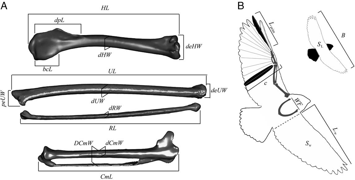
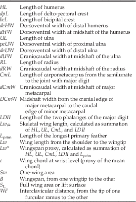
The measurements used as variables in this study are defined in Table 1 and depicted in Figure 1.
Measurements of wing elements used in this study (defined in Table 1). A, Skeletal forelimb elements: humerus (cranial aspect), ulna (dorsal aspect), radius (dorsal aspect), and carpometacarpus (dorsal aspect). B, Bird silhouette for illustrating the furcula and feathered wing measurements.

Definition of measurements of the forelimb elements used in this study, which are illustrated in Fig. 1.

Data Processing and Predictive Models
Data from modern birds were used to fit linear regression functions using the ordinary least-squares method (OLS), with B and S L as the response variable (y), and the measurements taken in forelimb skeletons and wing feathers as predictor variables (x). Given that a relationship of dependence for both B and S L on the x variables can be assumed, and given that prediction is the main objective of the regression analyses, the OLS method is the most adequate for deriving the equations (Gingerich et al. Reference Gingerich, Smith and Rosenberg1982; Sokal and Rohlf Reference Sokal and Rohlf1986; MacLeod Reference MacLeod2004; Smith Reference Smith2009; Campione and Evans Reference Campione and Evans2012). Furthermore, given that raw data for B, S L, and the skeletal measurements show positively skewed distributions, all data were log10-transformed in order to approximate a normal distribution and minimize the level of heteroscedasticity (Quinn and Keough Reference Quinn and Keough2001; Cawley and Janacek Reference Cawley and Janacek2010; however, see Packard et al. Reference Packard, Boardman and Birchard2009). However, the predicted log values obtained from least-squares regression could bias the results when they are retransformed to arithmetic units (Smith Reference Smith1993; Hayes and Shonkwiler Reference Hayes and Shonkwiler2006; Clifford et al. Reference Clifford, Cressie, England, Roxburgh and Paul2013). To avoid this potential bias, each retransformed value was multiplied by a correction factor known as the “ratio estimator” (Snowdon Reference Snowdon1991). In addition, plots of the residuals against predicted values were also examined to detect outliers.
Three types of regression were derived for estimating B and S L in order to analyze their predictive reliability: 1) single regressions using the best-correlated predictor variable; 2) principal component regressions, selecting those principal components significantly correlated to response variables (see details in Rawlings et al. Reference Rawlings, Pantula and Dickey1998; Serrano et al. Reference Serrano, Palmqvist and Sanz2015); and 3) multiple MRs, using all predictor variables (i.e., full model), as well as MR equations with predictors selected by automatic stepwise procedure (selection of x variables showing the highest correlation with the y variable in such a way that each step refits the model by introducing or dropping any predictor variable based on the contribution of its partial regression slope; see details in Mendoza et al. Reference Mendoza, Janis and Palmqvist2006). Statistical analyses were carried out using SPSS statistical package, Version 20 (IBM Corporation 2011).
Reliability of the Predictive Models
The predictive strength of the models is based on their accuracy (i.e., proximity between estimated and real values) and generalizability (i.e., predictive ability of the models on new data). The accuracy of the functions was evaluated using the following values: (Reference Alerstam, Rosén, Bäckman, Ericson and Hellgren1) the coefficient of determination adjusted for the number of predictor variables incorporated in the model (R 2 adj=1−[1−R 2][N−1]/[N−p], where N is sample size and p is the number of predictor variables, which number in the MR models was set according to the general rule N/p>10; see Darlington 1990); and (Reference Álvarez, Meseguer, Meseguer and Perez2) the percent prediction error (%PE=[observed–predicted]×100/predicted), which measures the degree of overestimation (%PE<0) or underestimation (%PE>0) for each particular observation. The sample mean of the absolute values of %PE, noted as |%MPE|, is the average percent deviation between predicted and observed values. This allowed the calculation of the average prediction intervals for B and S L as predicted value ± |%MPE| (Smith Reference Smith1984; Mendoza et al. Reference Mendoza, Janis and Palmqvist2006; Campione and Evans Reference Campione and Evans2012; Field et al. Reference Field, Lynner, Brown and Darroch2013).
Generalizability of the models was evaluated using two validation tests. A first validation was performed at the species level. Specimens of 25% of the species in the data set were randomly selected (the number of specimens corresponds to 20% of the whole sample) to conform a subsample for cross-validation (see detailed procedure in Hurvich and Tsai [Reference Hurvich and Tsai1990], MacNally [Reference MacNally2000], and Mendoza et al. [Reference Mendoza, Janis and Palmqvist2006]). The functions derived from the remaining 80% of specimens were used for obtaining the values (B and S L) of the specimens of the validating subsample, and |%MPE| value was calculated for them (i.e., |%MPE|VS-25%). Such a random subsample is appropriate for testing generalizability in models aimed at estimating extinct crown species. However, stem taxa are not a random assortment of crown species, as they fall outside the phylogenetic boundaries of the crown group. A second validation was performed to address this issue. Models derived from the neoavian specimens were used to predict B and S L values in all specimens of Galloanserae (the sister clade of Neoaves). The |%MPE| values calculated for Galloanserae (i.e., |%MPE|VS-GA) were used to test the stemward predictive strength of the models. In both approaches, the specimens of the validating subsamples were incorporated into the regression functions after cross-validation in order to include all measured individuals.
Potential Biases in the Regression Functions
Taxon Weighting
The crown families used in this study are represented by different numbers of species, which in turn are represented by different numbers of measured specimens. Such uneven sampling is known to bias the regressions when the scores of overrepresented and underrepresented families/species are not randomly distributed around the regression line. For this reason, we adjusted the functions weighting the richness of specimens within a species (each specimen contributed to the regressions as 1/N specimens per species) and species within families (1/N specimens per family). Their %MPE values were compared with those from unweighted regressions.
Multicollinearity
Redundant information between x variables included in a given MR model (i.e., multicollinearity) is known to have negative effects on the prediction (Mitchell-Olds and Shaw Reference Mitchell-Olds and Shaw1987; Bowerman and O’Connell Reference Bowerman and O’Connell1990). For this reason, the predictive strength of the MR equations was compared with noncollinear models, such as single regression and principal component regression. Multicollinearity was measured by the variance inflation factor (VIF), calculated for each variable x j as [1/(1−R 2)] from the OLS regression of x j against the remaining x variables (VIF values >10 suggest strong collinearity effects; see Kleinbaum et al. Reference Kleinbaum, Kupper and Muller1997).
Phylogenetic Nonindepedence
Any given sample of species does not meet the assumption of statistical independence due to the species’ historical relationships, and phylogenetically corrected methods should therefore be used (Felsenstein Reference Felsenstein1985; Harvey and Pagel Reference Harvey and Pagel1991). A calibrated cladogram of the modern birds included in the data set was constructed using MESQUITE software (Maddison and Maddison, Reference Maddison and Maddison2011). Tree topology and branch length of neognath species were obtained from Prum et al. (Reference Prum, Berv, Dornburg, Field, Townsend, Lemmon and Lemmon2015). Placement in the cladogram of those species not included in Prum et al. (Reference Prum, Berv, Dornburg, Field, Townsend, Lemmon and Lemmon2015) followed the family-level topology of this study; for clades unresolved by Prum’s phylogenetic hypothesis, the internal relationships followed specific references (see details in Supplementary Fig. S1). Phylogenetically independent contrasts (PICs) for each variable (Felsenstein Reference Felsenstein1985) were obtained using the PDA:PDTREE package (Midford et al. Reference Midford, Garland and Maddison2005). Standardized PICs versus their standard deviations were used to check whether branch lengths adequately fit the tip data (see Díaz-Uriarte and Garland Reference Díaz-Uriarte and Garland1996). In addition, given that the use of variables with a poor phylogenetic signal may be incorrect in statistical terms (Revell Reference Revell2010), the phylogenetic signal of the predictors was tested as follows: the squared length of each trait was statistically tested against 104 randomly generated trees in which terminal taxa were permuted while holding tree topology and branch lengths constant. Specifically, signal is significant if the number of steps between the basal node and the terminal branches of the tree analyzed are lower than in the random trees (see details in Laurin Reference Laurin2004).
Least-squares single regressions were derived for the PICs of each predictor variable against B and S L to deal with the nonindependence issue. PIC regressions were compared with OLS models for species means (uncorrected models) in order to check whether the scaling patterns within a phylogenetic context were not significantly different from a context in which the birds of the sample were independent (from a statistical point of view). PIC bivariate models are regressions through the origin (i.e., intercept=0). As residuals of this type of regression usually have a nonzero mean, straightforward comparisons with OLS may not be appropriate (Eisenhauer Reference Eisenhauer2003). For this reason, the difference between slopes from PICs and OLS was tested using the overlap of the 95% confidence intervals, obtained by bootstrapping (2000 replicates).
Selection of Variables: Scaling Patterns in Crown and Stem Groups
To derive predictive models for estimating the wingspan (B) of stem birds from a modern bird database, it is necessary to determine whether the portion of the body between the wings of stem birds scales similarly to the wingspan. This was tested following the calculations of Nudds and Rayner (Reference Nudds and Rayner2006) and by performing a reduced major axis (RMA) analysis between the width of furcula (WF) and a proxy of B that can be measured in several fossils, Lw* (HL+UL+CmL+LDII+L prim). This analysis was performed on a neognath’s data set of 326 individuals from 140 species (the data set of this study and additional data obtained from Viscor and Fuster [Reference Viscor and Fuster1987] and Bruderer et al. [Reference Bruderer, Peter, Boldt and Liechti2010]) and 10 extinct Mesozoic species. The confidence interval for the RMA slope was obtained through bootstrapping (2000 replicates). Subsequently, we also checked whether the variable L prim could be used for estimating B in stem birds, given that Wang et al. (Reference Wang, Nudds and Dyke2011) argued that some stem taxa had L prim values outside the neognath’s range, hence calling into question the predictive power of this variable. This was done by plotting the values of the ratio between L prim and the length of the skeletal wing (i.e., Lw sk=HL+UL+CmL+LDII) for each stem taxa and for a data set of neognaths composed of 256 individuals from 131 species and 67 families (additional data obtained from Viscor and Fuster [Reference Viscor and Fuster1987] and Bruderer et al. [Reference Bruderer, Peter, Boldt and Liechti2010]). Finally, the length of the wing’s skeletal elements (i.e., HL, UL, and CmL) was included in the MR functions derived for obtaining B values.
The MR models used for predicting the wing area (S L) of stem birds were derived from all forelimb variables, including c and L prim (see Table 1). Those variables that scale similarly in crown and stem groups were selected following the procedure of Serrano et al. (Reference Serrano, Palmqvist and Sanz2015). This approach minimizes the potential biases that could emerge from differences in morphological scaling patterns between living and extinct taxa and the effects of diagenetic compaction on fossil bones. The behavior of each x variable with respect to the remaining x variables was analyzed, and those that showed values in the fossil taxa outside the trends of Neognathae were discarded. The linear measurements were selected by plotting each measurement against the S L predicted from a combination of the remaining x variables. Subsequently, a regression line was fitted for modern birds in each plot, and those variables that scored within the 95% confidence intervals were selected for each stem group, allowing us to obtain particular subsets of predictors for them. Finally, the stepwise method was used in each subset for deriving the best multivariate functions. This procedure also helped to identify those skeletal measurements heavily affected by diagenetic compaction, which allows detection of individuals affected by taphonomy that would behave as outliers.
Post hoc Tests for Effects of Adaptive Changes
As in Serrano et al. (Reference Serrano, Palmqvist and Sanz2015), post hoc tests were performed over the MR functions obtained for evaluating the influence of locomotion adaptations on these equations and they were also compared with the best single regression (SR) models. The effects of flight mode on the prediction error (%PE) of B and S L were statistically tested by means of one-way analysis of variance (ANOVA). To do this, we classified modern birds into four categories according to their predominant behavior during aerial locomotion, following Pennycuick (Reference Pennycuick2008) and Bruderer et al. (Reference Bruderer, Peter, Boldt and Liechti2010): (1) continuous flapping, (2) flap and gliding, (3) flap and bounding, and (4) soaring. Given that these groupings differ in sample size, they could violate the ANOVA’s assumption of homoscedasticity, which was tested with the Levene’s test. In those cases in which homoscedasticity was rejected, the statistical differences between the locomotion groups were analyzed with the Welch’s test, a nonparametric procedure.
Calculation and Error Calibration of the Flight Parameters
As mentioned above, wing loading (WL) refers to the body weight supported by unit lift surface (i.e., BM g/S L, with g representing the acceleration of gravity). Then, using the estimates of BM obtained in Serrano et al. (Reference Serrano, Palmqvist and Sanz2015) and the S L values predicted from the MR functions developed in this study, we calculated the tentative WL value for each analyzed stem bird. Given that these WL estimates depend on two values (BM and S L) that have associated errors of estimation, we expect a greater margin of error for predicting WL. As we know the actual values of WL for specimens included in the modern data set, mean prediction errors could be estimated for this compound variable (i.e., %MPE, MPEVS-25%, and MPEVS-GA). This calculation was performed for each combination of predictive MR functions for BM and S L. The aspect ratio (AR) was obtained as the squared wingspan divided by the total wing surface (i.e., AR=B 2 /S L). As AR values also depend on two estimated values (i.e., B and S L) with an associated error, mean prediction errors (i.e., %MPE, MPEVS-25%, and MPEVS-GA) were also calculated for all combinations of predictive MR functions for B and S L. Such a procedure allows for calibration of the error of the compound variables (AR and WL) from the simple variables (B, S L, and BM). Furthermore, obtaining the |%MPE| values allowed us to delimit the confidence intervals for the estimates of WL and AR obtained for each basal bird.
Results
Predictive Ability from Different Regression Approaches (Issues from Multicollinearity, Taxon Weighting, and Automatic Stepwise Procedure).
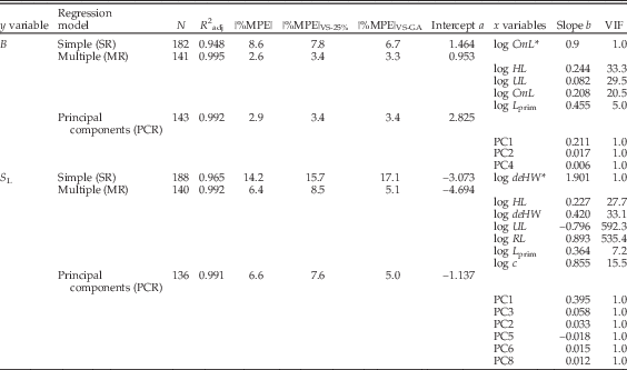
The best MRs derived for B and S L from the modern data set show a greater degree of multicollinearity when compared with both (Reference Alerstam, Rosén, Bäckman, Ericson and Hellgren1) single regressions of the best-correlated predictors (i.e., length of carpometacarpus for B and width of distal epiphysis of humerus for S L) and (Reference Álvarez, Meseguer, Meseguer and Perez2) regressions of the principal components (Table 2). In spite of this, MRs had a predictive strength that is notably higher than the corresponding single regressions (higher values of R 2 adj and lower MPEs). MRs also had slightly higher R 2 adj and predictive power on the whole data set (i.e., lower |%MPE|) than principal component regressions (Table 2). The errors in predicting B and S L values stemward were similar in MR and principal component regression (Table 2).
Ordinary least-squares (OLS) single regressions (SR) with the best-correlated x variables (*; i.e., higher Pearson coefficient), the best multiple regressions (MR), and the principal component regressions (PCR), derived to predict B and S L. N, number of individuals; R 2adj, coefficient of determination adjusted for the number of predictors included in the model; |%MPE|, mean percentage prediction error calculated over the whole data set; |%MPE|VS-25%, mean percentage prediction error calculated over the validating subsample of 25% species from the data set; |%MPE|VS-GA, mean percentage prediction error calculated using Galloansarae as validating subsample; VIF, variance inflation factor, 1/(1−R 2).

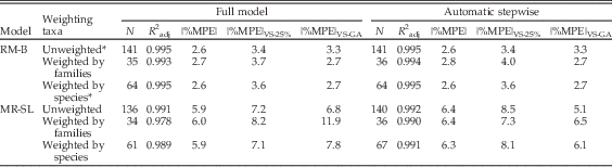
The R 2 adj values and MPE values of the unweighted MR models were similar or better than those values from taxonomically weighted MR models (Table 3).
Effects of the taxonomic weighting and the stepwise procedure on the prediction errors of the best MRs derived from the modern bird data set. |%MPE|, mean percentage prediction error calculated over the whole data set; |%MPE|VS-25%, mean percentage prediction error calculated over the validating subsample of 25% species from the data set; |%MPE|VS-GA, mean percentage prediction error calculated using Galloansarae as validating subsample. Asterisk (*) indicates that the stepwise procedure extracted the same function as the full model.

As expected, the reduction of variables included in a model generated by automatic stepwise resulted in a better-adjusted coefficient of determination (R 2 adj) when compared with the full model (Table 3). S L prediction errors on the whole data set (i.e., |%MPE|) were slightly lower in the models that included the full set of x variables. However, we found that the models generated by automatic stepwise increased the predictive power (at least by 1.7%) on new specimens placed stemward from Neoaves (|%MPE|VS-GA in Table 3).
Phylogenetic Nonindependence
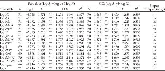
Diagnostics for suitability of PICs relative to the branch lengths of the cladogram were achieved in all variables, as shown by the lack of relationship between PICs and their corresponding standard deviations (p>0.05). The variables B, S L, and all forelimb measurements showed a highly significant phylogenetic signal in the tree of Neognathae (permutation tests: p<0.001 in all cases). This indicates that the use of phylogenetically corrected models, like PICs, derived from this data is statistically appropriate (Revell Reference Revell2010). Least-squares linear regressions with B as the response variable were highly significant in both regression approaches, PICs and OLS on the mean species values (permutation test: p<0.0001), showing an overlap in the corresponding confidence intervals for the slopes (Table 4). In all cases, phylogenetically corrected scaling relationships showed lower R 2 values than those adjusted from uncorrected data. Regressions for S L on the unstandardized SR functions and PICs were also highly significant in all cases (permutation test: p<0.0001), overlapping the confidence intervals for the slopes (Table 5). In addition, R 2 values of phylogenetically corrected functions were lower than R 2 values of the OLS regressions of species means, except in the cases of HL, RL, and CmL.
OLS single regressions obtained for each predictor variable against wingspan (B), using the means of species calculated from raw data and the appropriate phylogenetically independent contrasts (PICs). PICs assume a regression through the origin (a=0). Statistical significance of the regressions was checked by permutation tests with 10,000 replicates and 95% bootstrapped confidence intervals of the slopes (CI) are also shown. Slope difference significance between OLS raw data and OLS PICs were tested using Student’s t-test (α=0.05). For abbreviations of variables, see Table 1.

*** p<0.0001. ns, not significant (p>0.05).
OLS single regressions obtained for each predictor variable against wing area (S L), using the means of species calculated from raw data and the appropriate PICs. PICs assume a regression through the origin (a=0). Statistical significance of the regressions was checked by permutation tests with 10,000 replicates and 95% bootstrapped confidence intervals of the slopes (CI) are also shown. Slope difference significance between OLS raw data and OLS PICs were tested using Student’s t-test (α=0.05). For abbreviations of variables, see Table 1.

* 0.01<p<0.05; *** p<0.0001; ns, nonsignificant (p>0.05).
The overlapping of the confidence intervals of the slopes observed indicates that the morphological patterns depicted by the species sampled are not strongly driven by phylogeny; the variables can be considered statistically to be “taxon free.” Therefore, the nonindependence issue does not affect the phylogenetically uncorrected models. In addition, these models also showed higher predictive power.
Predictive Models for Wingspan
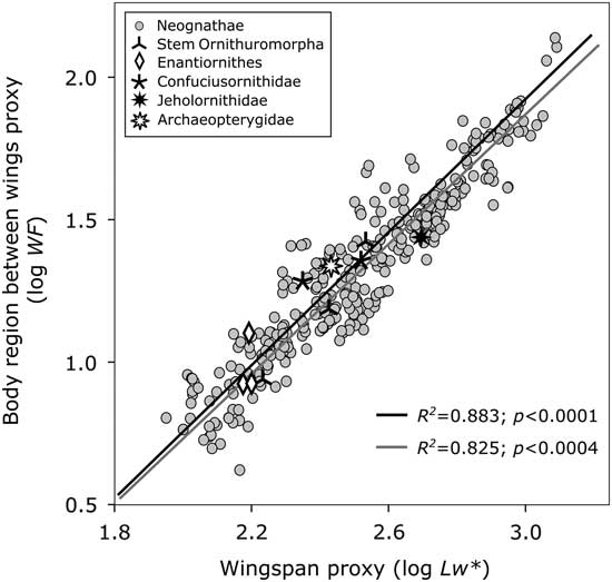
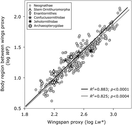
The relationship between the interclavicular distance (i.e., WF) and the proxy for wingspan (i.e., Lw*) in the sample of neognaths shows a slightly positive allometry (RMA slope=1.14; 95% confidence interval=1.10–1.18). As the slope of the stem birds analyzed (RMA slope=1.17; 95% confidence interval=0.72–1.49) is included in the confidence interval of modern birds, a similar scaling pattern can be assumed (Fig. 2). Then, the prediction of B values for non-neornithine birds is not affected by any possible differences in the interclavicular distance (i.e., the corporal region situated between the wings) between these birds and their living counterparts.
Relationship between interclavicular distance (WF) and a proxy of wingspan, Lw* (taken as the cumulative length of HL, UL, CmL, LDII, and L prim) in modern flying birds and those stem birds in which these variables could be unequivocally measured. The gray line corresponds to the RMA slope for Neognathae (log WF=1.142 log Lw* −1.555; N=326). The black line represents the RMA slope for stem birds (log WF=1.178 log Lw* −1.607; N=10). R 2 and the p-values of the regressions (obtained with permutation test with 10,000 replicates) are displayed in the graph.
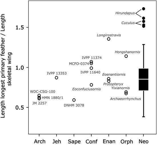
For all analyzed stem birds, the length of the longest primary feather (L prim) with respect to the sum of the lengths of the skeletal elements of the forelimb (Lw sk) is included in the range of variation of neognaths (Fig. 3). This suggests that the variable L prim has a potential use for generating models based on modern birds, therefore allowing the prediction of B in stem birds.
Proportion between the longest primary feather (L prim) and the length of the wing skeleton (Lw sk) in the main avian taxa. Abbreviations: Arch, Archaeopterygidae; Jeh, Jeholornithidae; Sape, Sapeornithidae; Conf, Confuciusornithidae; Enan, Enantiornithes; Orph, basal members of Ornithuromorpha; Neo, Neognathae. Box length in neognaths indicates the interquartile range (25th and 75th percentiles) and horizontal lines show the 5–95% confidence limits. Black points are outliers.

Three MR models for estimating B in extinct birds were derived (Table 6), showing very low prediction errors (|%MPE|: 2.6–7.4%; and |%MPE|VS-GA: 3.3–4.7%). The application of these models depends on the anatomical portions preserved in the fossils. The most complete model is MR-B1, because it includes the length of each wing element used to calculate wingspan except LDII. The function MR-B2 was applied to those fossils that do not preserve the wing feathers (i.e., the measurement of L prim was not available for them), which increases the uncertainty of the estimation. Finally, the model MR-B3 is useful to make predictions in the case of those fossils of basal birds that are less complete and cannot provide a CmL value; this has the poorest predictive power of the three models.
OLS MRs derived for predicting wingspan (B) in avian taxa. For abbreviations of variables, see Table 1. N, number of individuals; R 2 adj, coefficient of determination adjusted for the number of predictors included in the model; |%MPE|, mean percent prediction error calculated over the whole data set; |%MPE|VS-25%, mean percent prediction error calculated over the validating subsample (25% species); |%MPE|VS-GA=mean percentage prediction error calculated using Galloanserae as validating subsample.

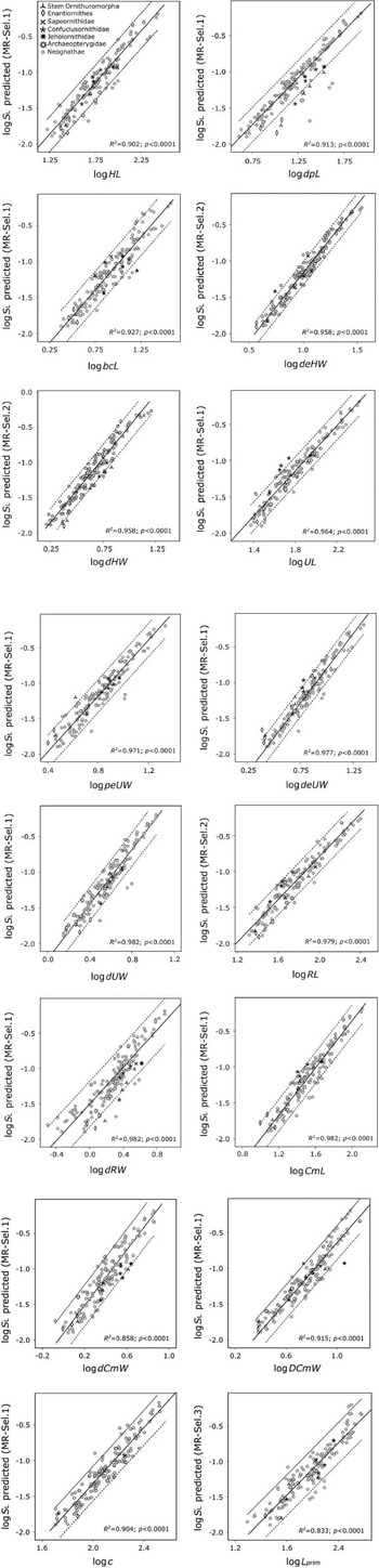
Predictive Models for Lift Surface
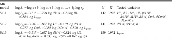
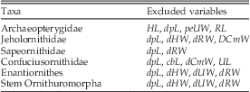
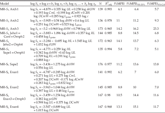
After selection for the predictor variables (Fig. 4, Table 7), several of them were excluded for deriving the specific functions for each stem taxa (Table 8). This results in 11 MR functions for predicting S L values (i.e., more than one for each of the six fossil groups; Table 9). The application of a given equation to a given fossil depends on which variables it preserves. The number of predictor variables included in the models ranged from two in the equation MR-SLArch3 to seven in both MR-SLArch1 and MR-SLEnan1. Their predictive error |%MPE| was less than 15% in all cases. Stemward validation suggests a good generalizability for the models selected, with 10 MR models having |%MPE|VS-GA values ranging from 5.1% to 13.8%, and one model doing notably worse than the others (23.3% in MR-SLArch3). The MR equations based on the highest skeletal completeness derived for Archaeopterygidae (MR-SLArch1), Enantiornithes (MR-SLEnan1), Sapeornithidae, and stem Ornithuromorpha (MR-SLSape1/MR-SLOrph1) have the highest predictive strength (|%MPE| and |%MPE|VS-GA ≈ 5–6%). In contrast, those functions based on fewer variables for Archaeopterygidae (MR-SLArch3), Enantiornithes (MR-SLEnan4), and Sapeornithidae (MR-SLSape2) were worse predictors (|%MPE| ≈ 11–14%; and |%MPE|VS-GA 11.7–23.3%).
Scaling of the anatomical variables against estimated wing surface (S L) in modern and stem birds. The biplots are used in the procedure of selection of variables for each basal group of Mesozoic birds (identified with different symbols). Each of 16 anatomical variables was plotted against a combination of the remaining variables used for estimating S L (Table 7). Each biplot shows the OLS regression line fitted for extant birds (gray circles) with the 95% confidence intervals for S L predictions (dotted lines), the R 2 value, and the p-value of the regression (obtained with permutation test with 10,000 replicates).

OLS MRs used in the procedure for selection of variables. Three functions to predict S L were obtained from different combinations of the anatomical predictors (MR Sel.1-3). The S L values obtained in these functions were plotted against each predictor variable to test and select those for specific stem taxa (Fig. 4 and Table 8).

Forelimb variables discarded after the selection procedure for predicting S L on each avian taxa.

OLS MRs obtained for predicting wing area (S L) in each avian taxon. For abbreviations of variables, see Table 1. For abbreviations of fossil taxa, see legend of Fig. 3. N, number of individuals; R 2 adj, coefficient of determination adjusted for the number of predictors included in the model; |%MPE|, mean percent prediction error calculated over the whole data set; |%MPE|VS-25%, mean percent prediction error calculated over the validating subsample (25% species); |%MPE|VS-GA, mean percentage prediction error calculated using Galloanserae as validating subsample.

Prediction Errors Derived from Adaptive Differences
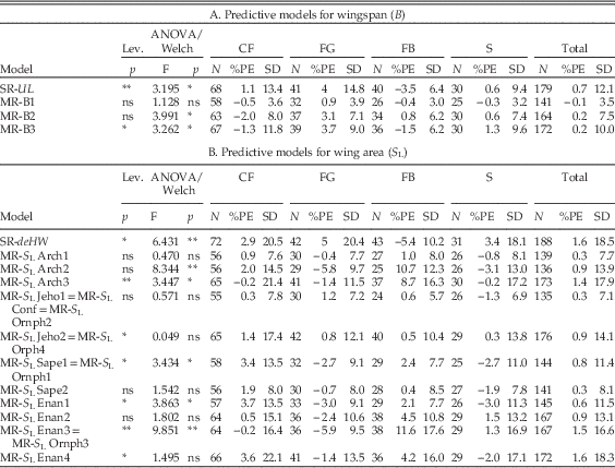
The post hoc analyses performed on the errors associated with the prediction of B values showed that the most predictive multivariate equation (i.e., MR-B1) was not affected by the flight mode of modern birds. Specifically, the ANOVA provided statistically nonsignificant results for the differences among groups of aerial locomotion (Table 10A). These differences, however, are significant in the other two MR equations (i.e., MR-B2 and MR-B3) and in the most predictive univariate function (i.e., SR from UL), which means that their B predictions are influenced by flight modality. However, the low mean %PE values and standard deviations obtained for each aerial group indicate that MR-B2 and MR-B3 minimize the influence of flight modality more than the best SR equation.
Effect of different aerial locomotion on the mean prediction error (%PE) values of the best SR equation and the MR models obtained. Flying mode abbreviations: CF, continuous flapping; FG, flap and gliding; FB, flap and bounding; S, soaring. For abbreviations of variables, see Table 1. When Levene’s test (Lev.) was nonsignificant, the difference between groups was tested by a one-way ANOVA. In other cases, Welch’s test was performed. For abbreviations of fossil taxa, see legend of Fig.3.

* 0.05> p>0.01; ** p<0.01; ns=p>0.05.
SD indicates the standard deviations for the mean values.
Table 10B shows that six of the 11 MR models derived for predicting S L are independent of the type of aerial locomotion, as their corresponding ANOVAs are nonsignificant. However, the best SR equation (i.e., deHW) and the five MR functions result in S L estimates that are affected by flight mode. As in the previous case, the influence of aerial locomotion is minimized in the MR functions with respect to the SR equations, as shown by the lower mean %PE values and standard deviations.
Calibrating the Aerodynamic Parameters: WL and AR
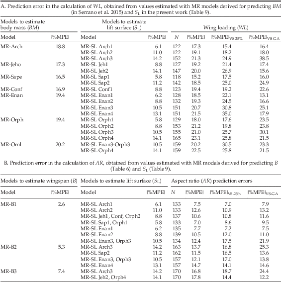
The WL values calculated from the estimates of BM and S L have a range of prediction errors between 15.2% and 23.1% (Table 11A). Taking into account the |%MPE| range from the MR models derived for predicting BM (16.5–20.2%) and S L (5.8–14.2%), the error accumulated for obtaining WL estimates can be considered quite low and depends mainly on the prediction error associated with the estimation of BM. However, it should be noted that two combinations of regression models (MR-Arch to estimate BM with MR-SLArch3 to estimate S L; and MR-Orph to body mass with MR-SL Orph3 to S L) gave values greater than 30% in the stemward validation.
Calibration of the cumulative prediction error on flight parameters.

On the other hand, the range of prediction errors for the AR values calculated from S L and B estimates fluctuates between 7.0% and 17.8% (Table 11B). Given that the |%MPE| ranges associated with the prediction of B values (2.6–7.4%) and S L values (5.8–14.2%), the cumulative error of the AR estimates can also be considered very low, and in this case it basically depends on the prediction error of S L. As in the previous case, combinations including MR-SL Arch3 to estimate SL resulted in the highest values for the stemward validation.
B, S L, WL, and AR Values in Mesozoic Stem Taxa
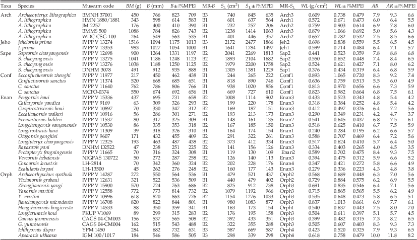
The MR functions obtained (Tables 6 and 9) were used to estimate B and S L values in the fossil specimens studied. These values and those obtained for BM (Serrano et al. Reference Serrano, Palmqvist and Sanz2015: Table 8) were used for calculating the WL and AR estimates for extinct birds (Table 12). The specimens of Archaeopterygidae show a range in WL values between 0.572 g/cm2 and 0.879 g/cm2, the values obtained for the Berlin and Solnhofen specimens of Archaeopteryx, respectively. The AR values obtained for these birds range from 5.0 to 7.9 (Solnhofen and London specimens, respectively). In the case of Jeholornithidae, the largest specimen sampled (V13274) is also the most loaded, and its AR value is lower than in the other sampled specimen (V13353), which is considered a juvenile (Zhou and Zhang Reference Zhou and Zhang2003). Similarly, the smallest specimen of Sapeornis, also considered a juvenile (DNHM 3078; Gao et al. Reference Gao, Chiappe, Zhang, Pomeroy, Shen, Chinsamy and Walsh2012), has the lowest values for WL (0.376 g/cm2) and AR (6.4). Larger specimens of Sapeornis show WL and AR ranging between 0.441 g/cm2 and 0.550 g/cm2 and 7.1 and 7.8, respectively. In contrast, the smallest (and oldest) sampled specimen of Confuciusornithidae (i.e., Eoconfuciusornis) presents WL and AR values higher than those for individuals of Confuciusornis. The confuciusornithid specimens analyzed show WL and AR ranging from 0.636 g/cm2 to 0.893 g/cm2 and from 5.5 to 8.3, respectively. In the case of Ornithothoraces, the WL values of enantiornithines range between 0.240 g/cm2 in Longirostravis and 0.59 g/cm2 in Protopteryx and Otogornis, while the AR values vary from 4.0 in Rapaxavis to 8.4 in Protopteryx. The basal members of Ornithuromorpha have WL values ranging between 0.399 g/cm2 and 0.837 g/cm2, which correspond to the values of Gansus (CAGS-04-CM003) and Jianchangornis, respectively. The lowest AR value (5.1) is estimated for Longicrusavis, while Apsaravis shows the highest value (10.0).
Estimates of the basic and compound variables for the specimens of Mesozoic stem taxa. The multiple regression model from which wingspan (B) and wing area (S L) were obtained, are also indicated (MR-B and MR-S L, from Tables 6 and 9). The body mass values (BM) obtained in Serrano et al. (Reference Serrano, Palmqvist and Sanz2015) are also included for a summary. The prediction errors (%MPEs) of wing loading (WL) and aspect ratio (AR) calculated on the modern data set are also shown for different combinations of B, S L, and BM estimates. Prediction intervals were calculated as predicted values ± |%MPE| values.

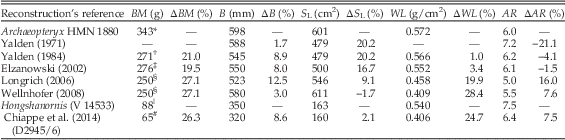
Table 13 shows the differences between the values of B, S L, WL, and AR estimated in this study and those provided by other authors using outline body reconstructions. It is evident from this comparison that our estimate of B for the Berlin Archaeopteryx (598 mm) differs more from the estimate obtained by Longrich (Reference Longrich2006) than from the estimates provided by Yalden (Reference Yalden1971, Reference Yalden1984), Elzanowski (Reference Elzanowski2002), and Wellnhofer (Reference Wellnhofer2008). In the case of S L, our estimate is similar to those of Wellnhofer (Reference Wellnhofer2008) and Longrich (Reference Longrich2006), but differs to a greater extent from those derived using the other two previous models (e.g., Yalden [Reference Yalden1971, Reference Yalden1984] and Elzanowski [Reference Elzanowski2002]). In regards to Hongshanornis, our estimates of B and S L are close to those provided by Chiappe et al. (Reference Chiappe, Zhao, O’Connor, Chunling, Wang, Habib and Cheng2014). Given that the specimen of Hongshanornis analyzed here (IVPP V14533) is not the same as the one used in the latter study (DNHM D2945/6), the small differences between these estimates can be interpreted as the result of intraspecific variation. A more important difference involves the BM values (i.e., 88 g vs. 65 g), which impact the values calculated for WL (i.e., 0.540 g/cm2 vs. 0.406 g/cm2).
Comparison between the estimates for Berlin’s Archaeopteryx and for Hongshanornis (two specimens) obtained using MR models (first line of each taxon) and outline body reconstructions. Superscript numbers indicate the method for obtaining BM values used in each study. The difference (in percent variation) between estimates from published reconstructions and estimates obtained in the present work is also shown.

* Multivariate allometric equation using six skeletal variables (ARCH), from Serrano et al. (Reference Serrano, Palmqvist and Sanz2015).
† Volumetric displacement.
‡ Univariate allometric equation using femoral width at midshaft (dFW), from Campbell and Marcus (Reference Campbell and Marcus1992).
§ Univariate allometric equation using dFW, from Yalden (Reference Yalden1984).
ǁ Multivariate allometric equation using seven skeletal variables (ORPH), from Serrano et al. (Reference Serrano, Palmqvist and Sanz2015).
# Univariate allometric equation using FL, from Peters and Peters (Reference Peters and Peters2009).
Discussion
From an aerodynamic point of view, the easiest approach to characterizing the wings of a bird is to measure their wingspan (B) and lift surface (S L) (Pennycuick Reference Pennycuick2008). For a given species, the values of these variables and the body mass (BM) allow for the calculation of two aerodynamic parameters, wing loading (WL) and aspect ratio (AR), known to influence flight speed, energy expenditure, and maneuverability (Viscor and Fuster Reference Viscor and Fuster1987; Rayner Reference Rayner1988; Norberg Reference Norberg2002; Alerstam et al. Reference Alerstam, Rosén, Bäckman, Ericson and Hellgren2007; Meseguer and Sanz-Andrés Reference Meseguer and Sanz-Andrés2007; Pennycuick Reference Pennycuick2008). This relation highlights the need to obtain reliable estimates of BM, B, and S L for the purpose of characterizing the flight of extinct avian taxa. Serrano et al. (Reference Serrano, Palmqvist and Sanz2015) provided regression models that allow estimating BM in a variety of stem birds. Previously, the only way to obtain B and S L estimates for stem birds was to use outline reconstructions of their wings, which were only available for fossils with well-preserved wing feathers. However, these reconstructions are relatively scarce and, with the recent exception of the basal ornithuromorph Hongshanornis (Chiappe et al. Reference Chiappe, Zhao, O’Connor, Chunling, Wang, Habib and Cheng2014), they have been mainly focused on the Berlin Archaeopteryx (e.g., Yalden Reference Yalden1971, Reference Yalden1984; Elzanowski Reference Elzanowski2002; Longrich Reference Longrich2006; Wellnhofer Reference Wellnhofer2008). Estimates of B and S L for extinct crown birds (e.g., Rando et al. Reference Rando, Alcover and Illera2010; Ksepka Reference Ksepka2014) have also been obtained using regression equations derived from skeletal measures in crown Aves. However, these predictive equations are subject to a number of sources of error and bias, especially for stem taxa, arising from statistical issues, phylogenetic history, locomotor adaptations, and diagenetic compaction (Serrano et al. Reference Serrano, Palmqvist and Sanz2015). Developing predictive models that are less influenced by these potential sources of error and bias, as those presented here, improves the reliability of the estimates.
The statistical limitations imposed by taxonomic unevenness in the modern data set (see Smith Reference Smith2002; Mendoza et al. Reference Mendoza, Janis and Palmqvist2006; De Esteban-Trivigno et al. Reference De Esteban-Trivigno, Mendoza and De Renzi2008) and the correlation between the predictor variables incorporated in the model (i.e., multicollinearity; see Mitchell-Olds and Shaw Reference Mitchell-Olds and Shaw1987; Bowerman and O’Connell Reference Bowerman and O’Connell1990; Quinn and Keough Reference Quinn and Keough2001) had no significant effects on the models’ ability to estimate B and S L. Additionally, the lack of generalizability of MRs, especially when obtained by the automatic stepwise procedure (see Smith Reference Smith2002; Whittingham et al. 2006), was not applicable to the MR functions for B and S L. In contrast, the stepwise procedure improved the predictive power stemward (i.e., on sister-taxa specimens that were not included to derive a given function).
In regard to the phylogenetic dependence of the data, the fact that the confidence intervals for the slopes of the PICs regressions overlapped with those derived from OLS on species means (Tables 4 and 5) suggests that phylogeny did not play a major role in the scaling patterns of flying birds for B and S L, at least for the forelimb elements measured. Such results indicate that the uncorrected models are not biased by phylogenetic dependence of the modern data set.
Given that it is not possible to directly examine the relationship between the dimensions of the forelimb elements and B or S L in the fossils, a certain degree of error must always be accepted by these types of paleobiological studies (see Carrano Reference Carrano2001; Smith Reference Smith2002; Packard et al. Reference Packard, Boardman and Birchard2009; Campione and Evans Reference Campione and Evans2012; Field et al. Reference Field, Lynner, Brown and Darroch2013). Such an error is compounded by the fact that progressively stemward taxa (in our case, Mesozoic non-neornithine birds) exhibit body plans that are progressively less similar to those depicted by the crown clade, which means that the applicability of the regressions is likely to decrease proportionately. For these reasons, it is important that the predictive equations derived from extant birds assume similar scaling patterns for the extinct species under consideration. To obtain values of B and S L as reliably as possible for the fossil specimens included here, we have taken into account the scaling relationships of the predictor variables in both modern and stem birds.
Wingspan (B) estimations depend on the length of the anatomical elements of the wing (i.e., humerus, ulna, carpometacarpus, major digit, and longest primary feather), the angles of the elbow and the wrist, and the length of the body region between the wings. Given that the length proportions between the main wing bones for stem birds are similar to those of modern birds (e.g., Middleton and Gatesy Reference Middleton and Gatesy2000; Dyke and Nudds Reference Dyke and Nudds2009; Benson and Choiniere Reference Benson and Choiniere2013), the lengths of these elements were used to derive regression models for predicting B values in stem Mesozoic birds. Similarly, the longest primary feather length (L prim) was used as an estimator of B, because our results indicate that stem taxa show L prim/Lw sk values within the range of neognaths (Fig. 3). These results are contrary to previous claims indicating that L prim was significantly shorter in some stem taxa (e.g., Archaeopterygidae and Enantiornithes) (Wang et al. Reference Wang, Nudds and Dyke2011). We argue that such disagreement stems in part from the fact that the limited taxonomic sample used by Wang et al. (Reference Wang, Nudds and Dyke2011)—50 species from a nonspecified number of families and orders—covers a smaller range of morphological variation than the one represented here—131 species from 67 families and 22 orders. In addition to the similarity in the proportions of the wing bones between modern and Mesozoic taxa, the angle of the elbow and wrist of the stretched wings of stem birds falls within the wide spectrum of modern birds, which ranges from very close to very open joint angles (e.g., swifts and many passerines, respectively; see Videler Reference Videler2005). Our results also show that the relationship between the proxies used in stem birds for the interclavicular distance (WF) and wingspan (Lw*) are within the neognath’s range, because the slope obtained for the 10 fossil specimens analyzed here is included in the confidence interval of the slope for modern birds (Fig. 2). Therefore, the prediction of B in stem birds using equations derived from modern birds is presumably not affected by morphological differences in the width of the corporal region situated between the wings. Finally, we obtained three MR models that allow estimating B in fossils with a varying degree of skeletal completeness. Unsurprisingly, the models that incorporate a high number of measures from wing elements have higher predictive power than those based on a low number (Table 6).
S L correlates with B because it spans the area of both wings and includes the area corresponding to the part of the body situated between the wings (Pennycuick Reference Pennycuick2008). In addition, S L correlates also with BM because it supports the bird’s weight in the air (Greenwalt Reference Greenwalt1975; Viscor and Fuster Reference Viscor and Fuster1987; Rayner Reference Rayner1988; Álvarez et al. Reference Álvarez, Meseguer, Meseguer and Perez2001; Norberg Reference Norberg2002; Sanz et al. Reference Sanz, Álvarez, Soriano, Hernández-Carrasquilla, Pérez-Moreno and Meseguer2002; Meseguer and Sanz-Andrés Reference Meseguer and Sanz-Andrés2007; Pennycuick Reference Pennycuick2008). Hence, the value of S L can be estimated from the same variables as B and BM, but it also depends on the wing chord (here considered the chord at wrist level, c). As in the case of the models derived for predicting BM by Serrano et al. (Reference Serrano, Palmqvist and Sanz2015), we have used a methodology whereby the osteological and feather measurements selected for each stem group were those that showed scaling patterns in extinct birds similar to those found among modern birds. This procedure generated 11 clade-specific MR functions that were used to predict S L for non-neornithine extinct birds. Within each stem taxa, several functions were derived for applying them to a given fossil, in accordance with the variables that the fossil preserved. Among these MR models, those that included the two variables related to the plumage (i.e., L prim and c) and some osteological measurements had the highest predictive power (Table 9).
Given that the variables used for deriving MR models for B and S L show similar scaling patterns in stem and modern birds, these models are robust against the bias generated by the deviations in body plans between crown and stem clades.
Moreover, a number of studies on the functional adaptations of modern birds have shown that the skeletal morphology of the wings is highly constrained by the dynamics of locomotion (e.g., Cubo and Casinos Reference Cubo and Casinos1998; De Margerie et al. Reference De Margerie, Sanchez, Cubo and Castanet2005; Habib and Ruff Reference Habib and Ruff2008; Hinic-Frlog and Motani Reference Hinic-Frlog and Motani2010; Simmons Reference Simmons2010; Bell and Chiappe Reference Bell and Chiappe2011; Simmons et al. Reference Simmons, Hieronymus and O’Connor2011; Dececchi and Larsson Reference Dececchi and Larsson2013), which could result in biased predictions of B and S L for new specimens, either extant or extinct ones. Compared with the most predictive univariate models, ulnar length (UL) and dorsoventral width of the distal humerus (deHW), the post hoc analyses indicate that a combined use of variables in the MR functions minimizes the effects of flying adaptations on the scaling between wing elements and B or S L (Table 10). Similar results were obtained for the effects of locomotion on the predictions of BM values (Serrano et al. Reference Serrano, Palmqvist and Sanz2015).
The effect of diagenetic compaction can alter the osteological dimensions of fossil birds, mainly the width of the ends of the long bones. The estimation of B values is not influenced by this potential bias, as this parameter is only estimated from longitudinal measures. In contrast, the S L values obtained from univariate models could be biased in severely compacted fossils. However, the use of a step-by-step methodology to obtain a specific MR model for each Mesozoic stem taxa reduces these potential biases, as in the case of the BM predictions (see Serrano et al. Reference Serrano, Palmqvist and Sanz2015).
Additional evidence on the reliability of the predictions obtained from the MR models derived here comes from the congruence of the values estimated for Archaeopteryx (Berlin specimen) and Hongshanornis (two different specimens) with those obtained by the most recent outline reconstructions (i.e., Wellnhofer Reference Wellnhofer2008; Chiappe et al. Reference Chiappe, Zhao, O’Connor, Chunling, Wang, Habib and Cheng2014). Furthermore, the B value of Archaeopteryx obtained by our MR models is also very close to those derived from reconstructed models (Yalden Reference Yalden1971, Reference Yalden1984; Elzanowski Reference Elzanowski2002), and its S L value approaches the one estimated by Longrich (Reference Longrich2006) on the basis of direct measurements of the Berlin specimen. The largest differences between previously published models are related to the BM values, which were previously calculated by either volumetric body displacement or univariate allometric inference (Table 13). The advantages of using MR models for obtaining reliable predictions of BM in stem birds were discussed in Serrano et al. (Reference Serrano, Palmqvist and Sanz2015).
Modern birds seem to display a pattern of “many-to-one mapping,” in which several distinct combinations of wing element lengths may result in wings that are functionally equivalent and show similar AR values. For this reason, combining evidence from different wing components allows reliable inferences on wing shape and function in neognaths to be derived (Hieronymus 2015). Therefore, we suggest that the selection of variables procedure developed in this study allows reliable stemward inferences of AR (and WL) values for extinct birds. Furthermore, in spite of the fact that the values predicted by MR models have an associated prediction error, calculation of flight parameters from them (i.e., WL and AR) does not result in an accumulation of this error. Hence, the empirical prediction errors of WL and AR resemble those of the basic variables estimated with the highest |%MPE| values (e.g., BM vs. WL and S L vs. AR; see Table 11). Because this is the first time in which WL and AR values have been calculated for an extensive data set, and the associated prediction errors are calibrated empirically, there is no reference for comparing the accuracy of the WL and AR estimates. Nonetheless, comparisons with the prediction errors provided for BM in previous studies (Serrano et al. Reference Serrano, Palmqvist and Sanz2015: Table 5 and references therein) indicate that these errors are relatively low. Therefore, the WL and AR estimates reported here can be considered suitable. In addition, given that the models to estimate BM, B, and S L are generalizable and robust against the sources of bias discussed above, this reliability can also be applied to the flight parameters derived from them.
Implications for the Flight of Early Aves
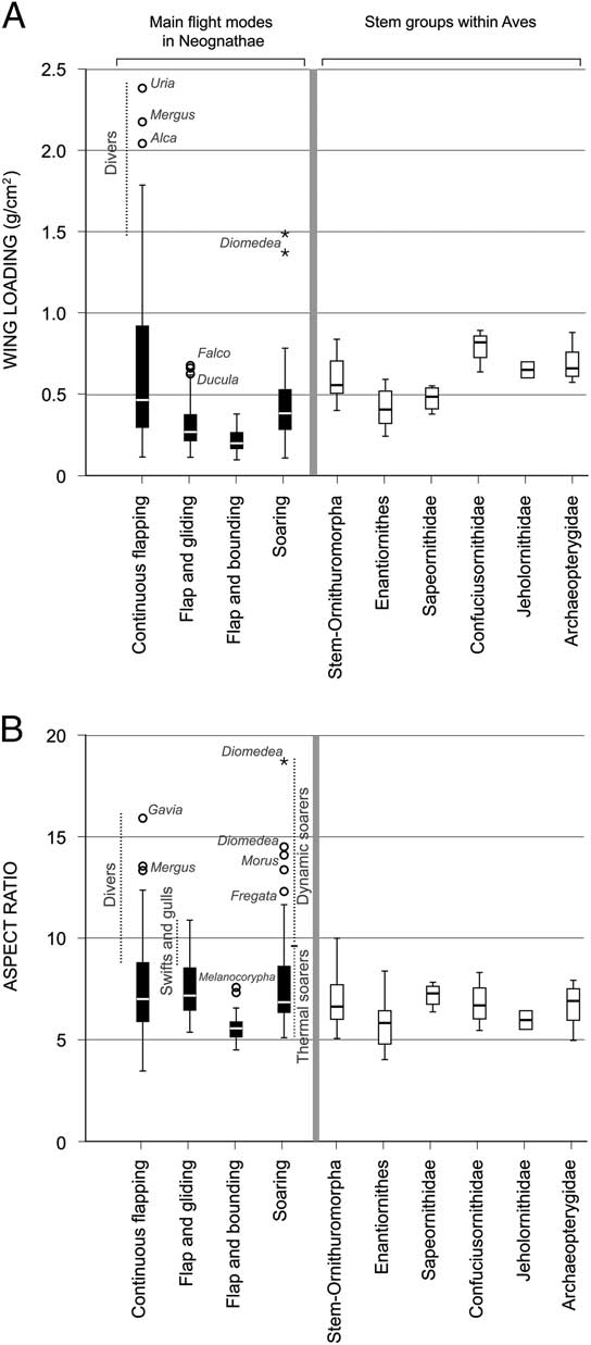
The estimates of WL and AR for the fossils included in this study show that these stem birds fall within the range of variation of modern birds (Fig. 5). In regard to WL, the range of variation of continuous flappers overlaps the ranges of the remaining modern flight modes. Diving birds (e.g., alcids, loons, and diving ducks), with high wing loads, fall in the uppermost range of the continuous-flapping spectrum. Specimens of Archaeopterygidae, Jeholornithidae, Confuciusornithidae, and early Ornithuromorpha show wing loads that are higher than those of Sapeornithidae and Enantiornithes. The latter clade includes the only stem birds that overlap with modern bounding fliers; the remaining stem birds included in this study overlap with other flight modes (i.e., continuous flapping, flap and glide, soaring). The WL values of sapeornithids overlap with the bulk of the soarers. With respect to AR, modern birds adapted to either dynamic soaring or diving have the highest values (>9.0). The AR estimates for stem birds ranged between 4.0 and 10.0, clearly within the range of most of modern birds (Fig. 5B). A combination of high wing loading and very high aspect ratio is not inferred in any of the fossil birds analyzed. This suggests that these birds were neither dynamic soaring nor diving specialists. Nonetheless, the combination of their WL and AR values indicate that these stem birds had evolved flight modes comparable to those of many modern birds. Furthermore, our data suggest that bounding flight, common among modern Passeriformes, could have been achieved by some enantiornithines.
Range of values for the aerodynamic variables calculated in the present study for stem avian taxa and flying neognaths. Modern birds are distributed according to their predominant flight mode. Each box plot represents one stem taxon or modern flight mode. Box length shows the interquartile range (25th and 75th percentiles). Whisker lengths indicate the 5–95% confidence limits. Unfilled circles represents individuals out of this range, and asterisks indicate outliers. A, Wing-loading values. B, Aspect ratio values.

Conclusions
Our MR models for predicting wingspan (B) and lift surface (S L) have a high prediction power and generalizability, which in turn indicate that they can provide accurate estimations. These models also minimize the potential biases that could result from statistical issues and differences in phylogenetic legacy, locomotor adaptations, and degree of taphonomic alteration. Furthermore, using models of variables that scale similarly in crown and stem taxa and that produce estimates similar to values obtained from direct measurements of preserved wing outlines provides indirect support for the accuracy of the values predicted for non-neornithine Aves. Therefore, accuracy, generalizability, and robustness of our MR models indicate that the B and S L values here obtained for stem birds are reliable. Given that the BM estimates are also minimally biased (Serrano et al. Reference Serrano, Palmqvist and Sanz2015), the values calculated for the aerodynamic parameters, WL (i.e., BM g/S L) and AR (i.e., B 2 /S L), can be considered minimally influenced by the biases mentioned above. In addition, although the estimations of BM, B, and S L carry an associated error, there is no cumulative error in the calculation of WL and AR from them; both aerodynamic parameters also show relatively low prediction errors. Our estimates of AR and WL show that stem birds could have flown using most of the flight modes known for modern birds, although we have found no evidence for either dynamic soarers or flighted divers (hovering was not analyzed). Evidence for bounding flight was found only among enantiornithines.
Acknowledgments
We dedicate this article to the memory of José Meseguer Ruiz, whose seminal work on aeronautical engineering will remain as a legacy and source of inspiration for future generations of scientists interested in animal flight. We thank N. Campione, A. Casinos, J. Cubo, J. Domínguez, B. Figueirido, A. Martín-Serra, J. Marugán-Lobón, J. A. Pérez-Claros, and two anonymous reviewers for providing suggestions and comments on earlier versions of this paper. We are also grateful to R. Faucett (University of Washington Burke Museum, Seattle, Washngton, U.S.A.), J. Barreiro (Museo Nacional Ciencias Naturales, Madrid), and Z. Zhou (Institute of Vertebrate Paleontology and Paleoanthropology, Beijing) for granting us with access to the specimens under their care; and to T. Hayden for providing editorial support. This work was supported by the Spanish Ministry of Economy and Competitiveness (Research Project CGL2011-30334), and by the agreement between the Natural History Museum of Los Angeles County (Los Ángeles, California, U.S.A.) and the Sierra Elvira Foundation (Granada, Spain).
Supplementary Material
Data available from the Dryad Digital Repository: http://dx.doi.org/10.5061/dryad.63k11