1 Introduction
Despite many years of research activity, the mechanism by which the turbulent structures in the jet generate noise is still a matter for debate. Since the seminal work of Lighthill (Reference Lighthill1952), significant progress has been made in terms of the understanding and modelling of jet noise (see e.g. Lilley Reference Lilley1991; Tam, Golebiowski & Seiner Reference Tam, Golebiowski and Seiner1996; Cavalieri et al. Reference Cavalieri, Jordan, Agarwal and Gervais2011 and Jordan & Colonius Reference Jordan and Colonius2013). Nevertheless, all the pieces of the puzzle have not yet been collected and further efforts are needed to have a clear picture of the jet noise production and propagation mechanisms.
Indeed, the investigation of the near region of the jet is essential to improve the knowledge of the jet physics and to identify the acoustic sources with the aim of developing noise control devices. As pointed out by Bonnet et al. (Reference Bonnet, Cole, Delville, Glauser and Ukeiley1994), the use of the proper orthogonal decomposition is a powerful tool to clarify the organised motion of the jet. To this extent, the POD was applied by Arndt, Long & Glauser (Reference Arndt, Long and Glauser1997) to pressure fluctuations measured in the near field in order to deduce the streamwise structure of the jet, the eigenfunctions being characterised by the amplification–saturation–decay trend of an instability wave. Nevertheless, the mere existence of POD modes does not imply that they have dynamical significance, especially in terms of noise generation (Freund & Colonius Reference Freund and Colonius2009). Indeed, the near-field energetic structures deduced by the POD are not necessarily representative of the noise-generating flow. This point was addressed by Picard & Delville (Reference Picard and Delville2000), who exploited the linear stochastic estimation to interpret the near-field pressure POD modes in terms of velocity field for the computation of the far-field noise. Nevertheless, an acoustical identification of the coherent flow structure educed by the POD is still far from being reached.
The discussion above motivated this work, whose main novelty lies in the presentation of a physical criterion for the interpretation of the near-field pressure POD modes in the streamwise direction in terms of hydrodynamic and acoustic pressures. Indeed, a microphone in the near field senses the fluctuations related to the non-radiating hydrodynamic pressure and the perturbations associated with the propagating acoustic pressure (Howes Reference Howes1960). The necessity of separating the pseudo-sound and sound components led to the development of different approaches (see Arndt et al.
Reference Arndt, Long and Glauser1997; Tinney & Jordan Reference Tinney and Jordan2008; Grizzi & Camussi Reference Grizzi and Camussi2012 and the recent papers by Mancinelli et al.
Reference Mancinelli, Pagliaroli, Di Marco, Camussi, Castelain and Léon2016, Reference Mancinelli, Pagliaroli, Di Marco, Camussi and Castelain2017b
). In this work the hydrodynamic or acoustic nature of the POD modes is assessed through the computation of the wavenumber–frequency spectrum of the near pressure field re-constructed using each POD mode. Specifically, on account of the phase velocity of the associated spectral energy bumps in the
 $k_{x}$
–
 $\unicode[STIX]{x1D714}$
domain, hydrodynamic, acoustic and ‘hybrid’ hydro-acoustic modes are detected for the first time. The propagation direction of the acoustic and hydro-acoustic radiating modes is identified through the correlation with the measured far-field noise. The analysis reveals a deeper overview of the sound generation and provides a range of
 $k_{x}$
and
 $\unicode[STIX]{x1D714}$
to be manipulated by control devices in order to reduce the acoustic emissions, the application of closed-loop control systems to experimental data being still a challenging task for the future, as recently pointed out by Sasaki et al. (Reference Sasaki, Cavalieri, Silvestre, Jordan, Tissot and Biau2017).
The paper is organised as follows. In § 2 a brief description of the experiment is given, whereas § 3 is devoted to the proper orthogonal decomposition of the near pressure field. The identification of the hydrodynamic, acoustic and hybrid modes through the wavenumber–frequency spectrum is presented in § 4. Conclusions are addressed in § 5.
2 Experimental set-up
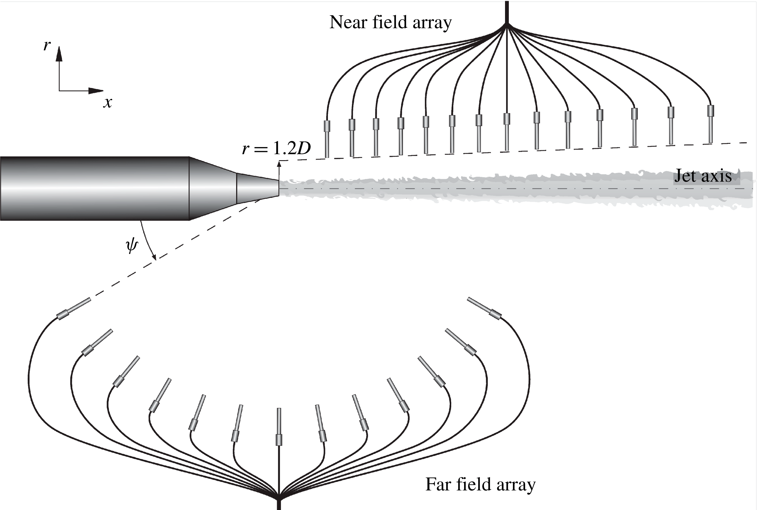
Experiments were carried out in the anechoic wind tunnel in the Centre Acoustique of Laboratoire de Mécanique des Fluides et d’Acoustique at the École Centrale de Lyon. Simultaneous near- and far-field pressure measurements were performed on a single-stream jet for Mach numbers
 $M_{j}=0.6$
and 0.9, to which correspond nozzle diameter-based Reynolds numbers of
 $7.5\times 10^{5}$
and
 $1.2\times 10^{6}$
, respectively. The 14-microphone array in the near field was placed in the so-called linear hydrodynamic regime (Suzuki & Colonius Reference Suzuki and Colonius2006) on a line following the jet spreading angle, the intercept of this line with the nozzle exit plane being at a radial distance
 $r/D=1.2$
from the jet axis. The microphones locations in the streamwise direction spanned an axial distance range
 $x/D=[2,8.7]$
. The 13-microphone array in the far field was located on a circular arc at a radial distance
 $r/D=40$
from the nozzle exhaust spanning a polar angle range
 $\unicode[STIX]{x1D713}=[30^{\circ },150^{\circ }]$
, the polar angle being defined positive in the upstream direction. A sketch of the experimental set-up as well as a scheme of the microphones disposition is shown in figure 1.
Sketch of the experimental set-up and microphones disposition.

The pressure fluctuations induced by the jet were measured by PCB 377B01 microphones. Time signals were acquired by National Instruments PXI-4472 system with a sampling frequency of 51.2 kHz for an acquisition time of 10 s. A preliminary test campaign was carried out to assess the accuracy of the experimental data. The acquisition parameters were carefully chosen in order to have an interval confidence of 99 % with a maximum uncertainty of 2 % for the evaluation of the statistical moments of interest, i.e. up to the fourth order (Tropea, Yarin & Foss Reference Tropea, Yarin and Foss2007; Mancinelli, Di Marco & Camussi Reference Mancinelli, Di Marco and Camussi2017a ).
For a more detailed description of the experimental set-up and a qualification of the jet facility the reader may refer to Mancinelli et al. (Reference Mancinelli, Pagliaroli, Di Marco, Camussi and Castelain2017b ).
3 Proper orthogonal decomposition of the near pressure field
For a comprehensive review on mathematical aspects of proper orthogonal decomposition and its application to turbulent flows the reader may refer to the large body of literature (e.g. Berkooz, Holmes & Lumley Reference Berkooz, Holmes and Lumley1993). In this work the POD is applied to the near pressure field
 $p(x,t)$
in the streamwise direction
 $x$
as in Arndt et al. (Reference Arndt, Long and Glauser1997) and Picard & Delville (Reference Picard and Delville2000). The Fredholm integral eigenvalue problem reduces to the following:
 $$\begin{eqnarray}\int _{D_{x}}R(x,x^{\prime })\unicode[STIX]{x1D6F7}_{n}(x^{\prime })\,\text{d}x^{\prime }=\unicode[STIX]{x1D706}_{n}(x)\unicode[STIX]{x1D6F7}_{n}(x),\end{eqnarray}$$
where
 $R(x,x^{\prime })$
is the auto-covariance matrix of the pressure field,
 $\unicode[STIX]{x1D6F7}_{n}(x)$
and
 $\unicode[STIX]{x1D706}_{n}(x)$
are the eigenfunctions and eigenvalues, respectively. It has to be underlined that
 $N=14$
modes are obtained for the present case, being 14 the number of microphones of the near-field array. The approximated space–time pressure field
 $\tilde{p}(x,t)$
can be recovered by summing all the POD modes, as reported in the following:
 $$\begin{eqnarray}\tilde{p}(x,t)=\mathop{\sum }_{n=1}^{N}\tilde{p}_{n}(x,t)=\mathop{\sum }_{n=1}^{N}a_{n}(t)\unicode[STIX]{x1D6F7}_{n}(x),\end{eqnarray}$$
where
 $a_{n}(t)$
are the projection coefficients of the near pressure field over the eigenfunctions, as formally defined in the following:
 $$\begin{eqnarray}a_{n}(t)=\int _{D_{x}}p(x,t)\unicode[STIX]{x1D6F7}_{n}(x)\,\text{d}x.\end{eqnarray}$$
In reference to (3.2), it has to be pointed out that the mean pressure is zero since the microphones measure only the fluctuating pressure.
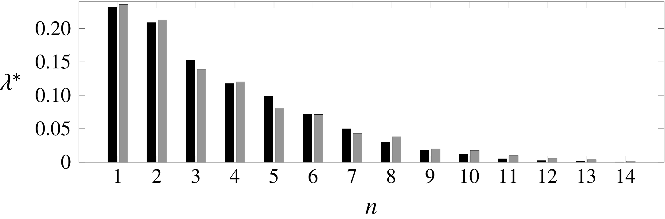
Figure 2 shows the normalised eigenvalues
 $\unicode[STIX]{x1D706}^{\ast }$
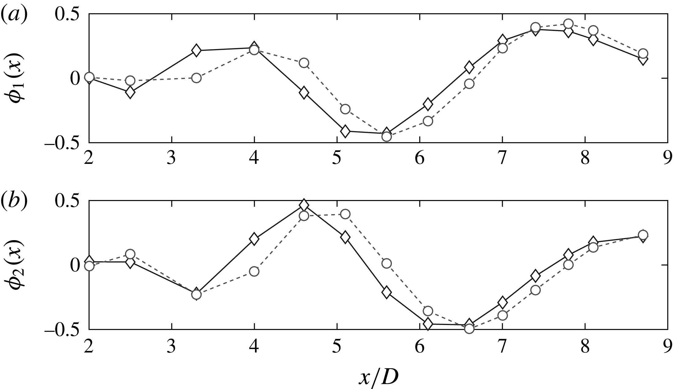
for both jet Mach numbers, the normalisation being achieved by dividing each eigenvalue by the sum of all the eigenvalues. As outlined by Arndt et al. (Reference Arndt, Long and Glauser1997), the eigenvalues provide an estimation of the coherent energy embedded in each POD mode. It is observed that the eigenvalue spectrum is almost independent of the jet Mach number and that the energy is distributed on a wide range of modes showing an exponential-like decay. The evolution along the streamwise direction of the first two POD modes, that are the most energetic ones, is represented in figure 3 for both
 $M_{j}$
. The trend is qualitatively in agreement with the typical instability wave shape reported by Arndt et al. (Reference Arndt, Long and Glauser1997) and Picard & Delville (Reference Picard and Delville2000). As for the eigenvalues, no significant effect of the jet Mach number can be detected.
Normalised eigenvalues for both jet Mach numbers: black bars refer to
 $M_{j}=0.6$
, grey bars to
 $M_{j}=0.9$
.

Trend of the first two POD modes along the streamwise direction for both jet Mach numbers: ♢ refer to
 $M_{j}=0.6$
, ○ to
 $M_{j}=0.9$
. (a) First POD mode, (b) second POD mode.

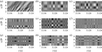
The space–time map of the original near pressure field and the re-constructed pressure fields using each POD mode is shown in figure 4. For the sake of brevity, the case
 $M_{j}=0.6$
was considered here as well as the first 8 POD modes for the re-construction of the space–time pressure fields. The re-constructed pressure fields show an organised structure, that is a chessboard-like pattern with characteristic wavelengths and time scales strongly dependent on the POD mode considered. It has to be pointed out that the characteristic wavelengths appear to change with the streamwise position, the resulting pattern being non-uniform in space.
Space–time map of the original near pressure field
 $p(x,t)$
and the re-constructed pressure fields
 $\tilde{p}_{n}(x,t)$
using each POD mode for jet Mach number
 $M_{j}=0.6$
. (a)
 $p(x,t)$
, (b)
 $\tilde{p}_{1}(x,t)$
, (c)
 $\tilde{p}_{2}(x,t)$
, (d)
 $\tilde{p}_{3}(x,t)$
, (e)
 $\tilde{p}_{4}(x,t)$
, (f)
 $\tilde{p}_{5}(x,t)$
, (g)
 $\tilde{p}_{6}(x,t)$
, (h)
 $\tilde{p}_{7}(x,t)$
, (i)
 $\tilde{p}_{8}(x,t)$
.

4 Identification of hydrodynamic, acoustic and hybrid modes
The chessboard-like pattern of the re-constructed pressure fields with different wavelengths and time scales suggests that the energy content of the associated wavenumber–frequency spectrum should be concentrated on a well-defined
 $k_{x}$
–
 $\unicode[STIX]{x1D714}$
region. The hydrodynamic or acoustic nature of the re-constructed
 $\tilde{p}_{n}(x,t)$
, and hence of the associated POD modes, can be assessed based on the location of the spectral energy in the
 $k_{x}$
–
 $\unicode[STIX]{x1D714}$
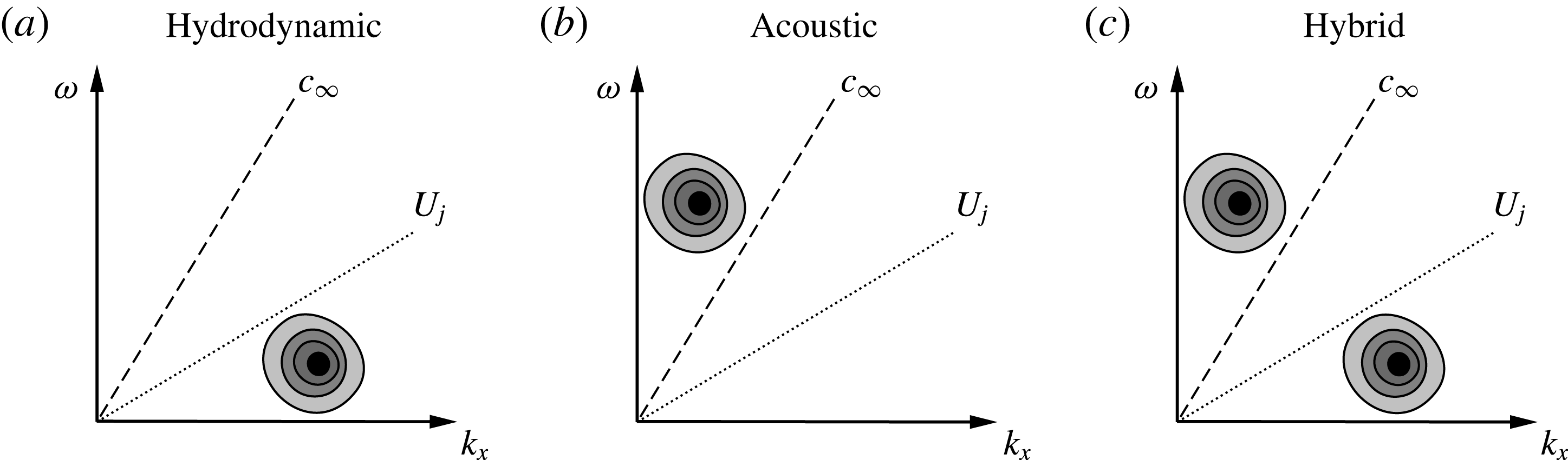
domain and on account of its phase velocity. According to Tinney & Jordan (Reference Tinney and Jordan2008), POD modes generating pressure fields characterised by a spectral energy bump with a phase velocity lower than the ambient speed of sound and of the order of the jet velocity are identified as hydrodynamic. On the other hand, POD modes providing re-constructed pressure fields with a phase velocity greater than or equal to the speed of sound are identified as acoustic. The re-constructed pressure fields whose wavenumber–frequency spectrum exhibit several energy bumps in the
 $k_{x}$
–
 $\unicode[STIX]{x1D714}$
domain having phase velocities greater and lower than the speed of sound are associated with hydro-acoustic or ‘hybrid’ modes. A schematic representation of the identification process reported above is depicted in figure 5.
Scheme of interpretation of the POD modes based on the location of the spectral energy in the
 $k_{x}$
–
 $\unicode[STIX]{x1D714}$
domain: (a) hydrodynamic, (b) acoustic, (c) hydro-acoustic or hybrid.

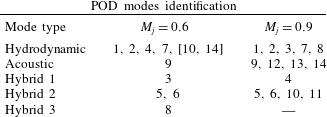
Three types of hybrid modes were detected. The mode denoted as hybrid 1 presented four spectral energy bumps, one of them having a phase velocity of the order of the speed of sound. On the contrary, the modes denoted as hybrid 2 and 3 presented two energy bumps, one bump having a phase velocity greater than or equal to the speed of sound.
On account of the topology of the
 $k_{x}$
–
 $\unicode[STIX]{x1D714}$
spectrum, the nature of each POD mode for both
 $M_{j}$
is summarised in table 1. The mode topology is analogous for both
 $M_{j}$
, with the exception of the hybrid 3 mode, this type of mode being detected only for
 $M_{j}=0.6$
. It has to be pointed out that the identification of the mode type does not have the same numbering order between the two
 $M_{j}$
, the numbering order being dependent on the energy of each mode. As expected, the first POD modes, that are the most energetic ones, exhibit a hydrodynamic nature. It is interesting to underline that the number of the acoustic modes is larger for
 $M_{j}=0.9$
, this result being related to the higher sensitiveness of the acoustic pressure to the jet Mach number variation (Mancinelli et al.
Reference Mancinelli, Pagliaroli, Di Marco, Camussi and Castelain2017b
).
Summary of the types of POD modes detected based on the phase velocity of the
 $k_{x}$
–
 $\unicode[STIX]{x1D714}$
spectrum of the re-constructed
 $\tilde{p}_{n}(x,t)$
for both jet Mach numbers.

The wavenumber–frequency spectrum of the re-constructed pressure fields are reported in the following. Each type of mode described above is presented and physically interpreted. The two-dimensional (2-D) Fourier transform of the space–time pressure fields is computed as follows:
 $$\begin{eqnarray}\hat{p}_{n}(k_{x},\unicode[STIX]{x1D714})=\int _{-\infty }^{+\infty }\int _{-\infty }^{+\infty }\tilde{p}_{n}(x,t)W(x)W(t)\text{e}^{-\text{i}(k_{x}x+\unicode[STIX]{x1D714}t)}\,\text{d}x\,\text{d}t,\end{eqnarray}$$
where
 $W(x)$
and
 $W(t)$
are Hamming windowing functions in the space and time domains, respectively. The wavenumber–frequency spectrum is given by the following:
 $$\begin{eqnarray}\hat{P}_{n}(k_{x},\unicode[STIX]{x1D714})=\hat{p}_{n}(k_{x},\unicode[STIX]{x1D714})\hat{p}_{n}^{\ast }(k_{x},\unicode[STIX]{x1D714}).\end{eqnarray}$$
The 2-D spectra are presented in dimensionless form, the normalisation being achieved by dividing the spectrum by the spectral energy peak. Furthermore, the frequencies are reported in terms of Strouhal number based on the nozzle diameter and the jet velocity, whereas the wavenumber is normalised by multiplying by the nozzle diameter.
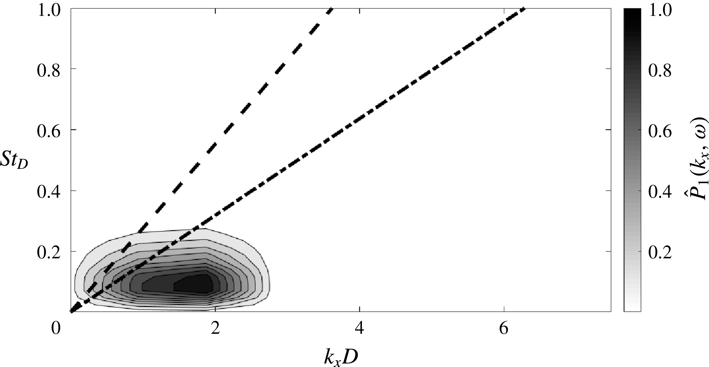
Figure 6 shows the
 $k_{x}$
–
 $\unicode[STIX]{x1D714}$
spectrum of a hydrodynamic mode. As an example the re-constructed
 $\tilde{p}_{1}(x,t)$
for
 $M_{j}=0.6$
was considered here. Only positive wavenumbers and frequencies are shown, the spectrum being symmetric with respect to the origin. As expected, the energy content is concentrated on a well-defined
 $k_{x}$
–
 $\unicode[STIX]{x1D714}$
band. Specifically, the spectral energy bump has a characteristic phase velocity lower than the jet velocity, the associated POD mode being identified as hydrodynamic.
Wavenumber–frequency spectrum of
 $\tilde{p}_{1}(x,t)$
for
 $M_{j}=0.6$
, whose associated POD mode is identified as hydrodynamic. Dashed line refers to the speed of sound, dash-dotted line to the jet velocity.

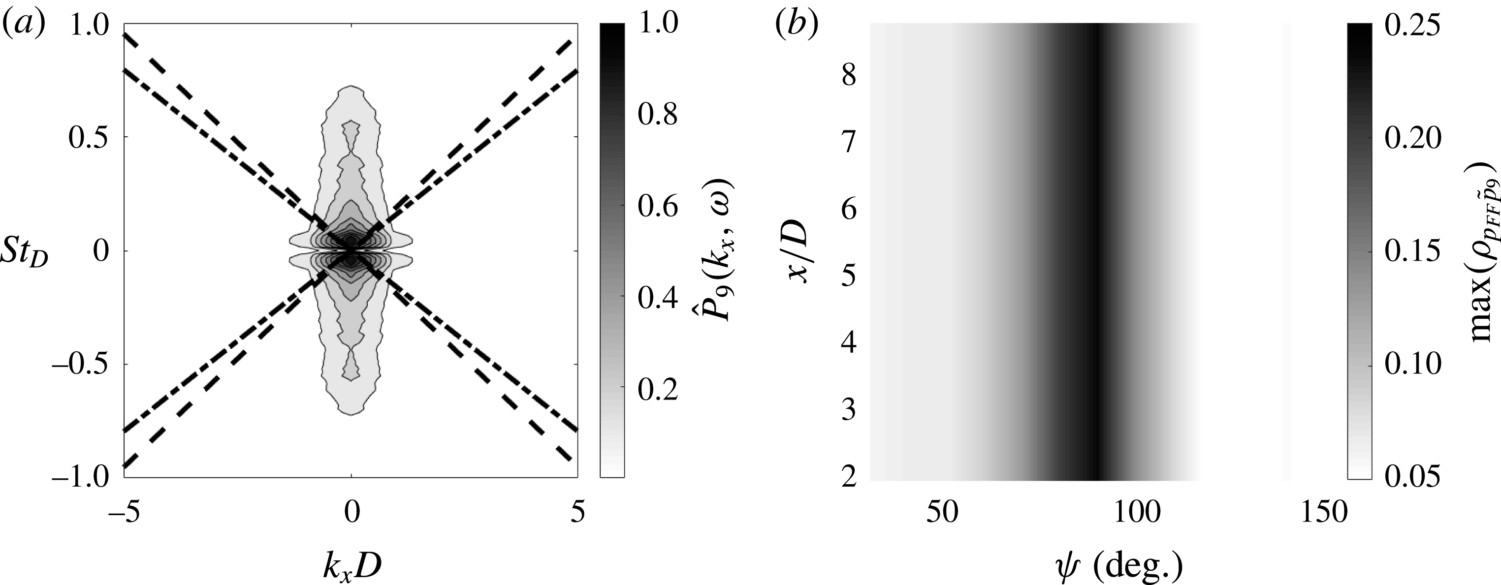
Figure 7(a) shows the
 $k_{x}$
–
 $\unicode[STIX]{x1D714}$
spectrum of
 $\tilde{p}_{9}(x,t)$
for
 $M_{j}=0.9$
. For the sake of clarity of the representation both negative and positive wavenumbers and frequencies are reported. It is observed that the spectral energy bump is characterised by a phase velocity that is much larger than the speed of sound, this feature suggesting the acoustic nature of the associated POD mode. It is interesting to point out that the associated phase velocity tends to infinity, thus indicating acoustic waves propagating orthogonal to the near-field microphone array axis and hence in the sideline direction in the far field. Such assertion is further supported by computing the cross-correlation between the far-field pressure and the re-constructed near-field pressure. Figure 7(b) shows the contour map of the cross-correlation coefficient peaks for all the near-field streamwise positions and all the far-field polar positions. It is observed that large correlation values are detected for all the axial positions only for polar angles in the neighbourhood of
 $\unicode[STIX]{x1D713}=90^{\circ }$
in the far field, thus confirming the preferential propagation direction in the sideline.
(a) Wavenumber–frequency spectrum of
 $\tilde{p}_{9}(x,t)$
for
 $M_{j}=0.9$
, whose associated POD mode is identified as acoustic. Dashed lines refer to the speed of sound, dash-dotted lines to the jet velocity. (b) Cross-correlation coefficient peak map between far-field pressure and re-constructed
 $\tilde{p}_{9}(x,t)$
for
 $M_{j}=0.9$
at all the axial and polar positions.

(a) Wavenumber–frequency spectrum of
 $\tilde{p}_{4}(x,t)$
for
 $M_{j}=0.9$
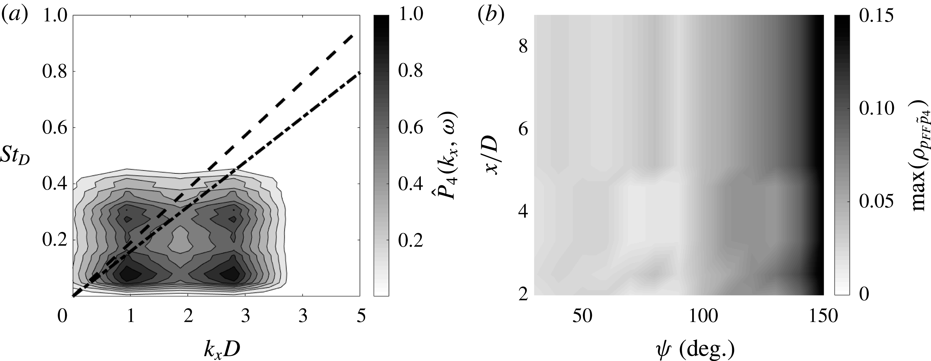
, whose associated POD mode is identified as hybrid 1. Dashed line refers to the speed of sound, dash-dotted line to the jet velocity. (b) Cross-correlation coefficient peak map between far-field pressure and re-constructed
 $\tilde{p}_{4}(x,t)$
for
 $M_{j}=0.9$
at all the axial and polar positions.

The wavenumber–frequency spectrum of the re-constructed
 $\tilde{p}_{4}(x,t)$
for
 $M_{j}=0.9$
is represented in figure 8(a), the associated POD mode being of the hybrid 1 type. Four main energy bumps are detected, one of them having a phase velocity of the order of the speed of sound. Such a behaviour implies the presence of acoustic waves travelling parallel to the near-field array axis and thus suggesting a downstream preferential propagation direction in the far field. The cross-correlation coefficient peak map between the far-field noise and the re-constructed
 $\tilde{p}_{4}(x,t)$
was computed for all
 $x/D$
and
 $\unicode[STIX]{x1D713}$
, its representation being reported in figure 8(b). It is clear that larger correlation levels are found for increasing polar angles, thus confirming the preferential radiation in the aft arc.
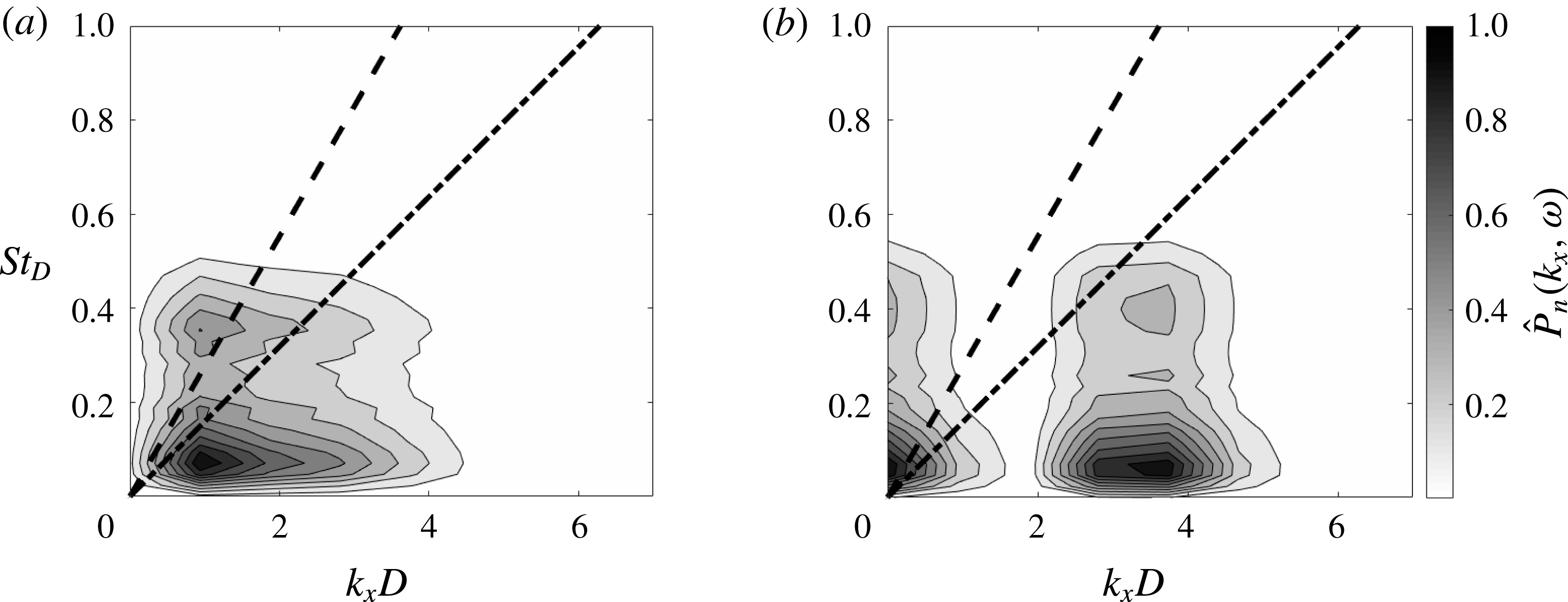
The
 $k_{x}$
–
 $\unicode[STIX]{x1D714}$
spectra of
 $\tilde{p}_{6}(x,t)$
and
 $\tilde{p}_{8}(x,t)$
for
 $M_{j}=0.6$
are shown in figure 9, the associated POD modes being of hybrid 2 and 3 types, respectively. The hybrid 2 mode is characterised by two energy bumps at the same wavenumber but different frequency, one bump having a phase velocity close to the speed of sound and being related to acoustic perturbations propagating in the downstream direction. The hybrid 3 mode exhibits two main bumps at the same
 $f$
with a different
 $k_{x}$
, the associated acoustic content having a phase velocity tending to infinity and hence being related to acoustic waves radiating in the sideline direction.
Wavenumber–frequency spectrum for
 $M_{j}=0.6$
: (a)
 $\tilde{p}_{6}(x,t)$
, whose associated POD mode is identified as hybrid 2; (b)
 $\tilde{p}_{8}(x,t)$
, whose associated POD mode is identified as hybrid 3. Dashed line refers to the speed of sound, dash-dotted line to the jet velocity.

5 Conclusions
In this paper the proper orthogonal decomposition of the near pressure field in the streamwise direction was performed. The POD modes have been interpreted in terms of their hydrodynamic or acoustic nature through the computation of the wavenumber–frequency spectrum of the re-constructed space–time pressure fields using each POD mode. The identification of the nature of the modes was achieved on account of the localisation in the
 $k_{x}$
–
 $\unicode[STIX]{x1D714}$
domain of the spectral energy bump through the comparison of its characteristic phase velocity with the ambient speed of sound. To the best of the authors’ knowledge, this represents the first attempt to provide a criterion for the physical interpretation and for the attribution of dynamical significance of the pressure POD modes in terms of representativeness of the noise generating flow.
The analysis of the topology of the
 $k_{x}$
–
 $\unicode[STIX]{x1D714}$
spectrum of each re-constructed pressure field revealed the presence of three classes of modes: hydrodynamic, acoustic and hydro-acoustic or hybrid. The hydrodynamic and acoustic modes were characterised by a spectral energy bump with a phase velocity of the order of the jet velocity and greater than or equal to the ambient speed of sound, respectively. The hybrid modes exhibited several energy bumps with different phase velocities. Three types of hybrid modes were detected based on the topology of the wavenumber–frequency spectrum. The propagation direction in the far field of the radiating acoustic content of the POD modes was investigated establishing a causality relation through the computation of the cross-correlation with the measured far-field noise. Specifically, modes associated with noise emissions radiating in the downstream/sideline direction, i.e. related to sound emissions from large/fine scale turbulent structures, were identified for the first time.
Future developments of the present work will involve a better definition of the role of the hybrid modes in the jet noise production in order to shed light on the link between the noise-generating hydrodynamic turbulent structures and the resulting acoustic perturbations. This result could be achieved by a band-pass filtering of the hydrodynamic and acoustic components embedded in the hybrid modes in order to establish a coupling or causality relation between the two pressure components. Such an application could permit to identify a trace of the noise generation mechanism highlighting the characteristic wavelengths and time scales of the flow structures associated with the acoustic emissions. This point is essential to implement passive or active noise control strategies having an effect on the energy content in the
 $k_{x}$
–
 $\unicode[STIX]{x1D714}$
band more efficient in terms of noise emissions.
Finally, it is authors’ opinion that the new approach presented herein can represent a framework for several further research activities in the field of physical understanding of jet noise, reduced-order modelling of jet flow dynamics and noise control.
Acknowledgements
The authors acknowledge the support of the EU Collaborative project ORINOCO (ACP0-GA-2010-266103). M.M. and R.C. also acknowledge the partial support of the EU Collaborative project JERONIMO (ACP2-GA-2012-314692). Both the projects are funded under the 7th Framework Programme.