Modern studies of legislative behavior focus upon the relationship among the policy preferences of legislators, institutional arrangements, and legislative outcomes. In spatial models of legislatures, policies are represented geometrically, as points in a low-dimensional Euclidean space. Each legislator has a most preferred policy or ideal point in this space and his or her utility for a policy declines with the distance of the policy from his or her ideal point; see Davis, Hinich, and Ordeshook (1970) for an early survey.
The primary use of roll call data—the recorded votes of deliberative bodies1
The same model is applicable to courts, though the data are called “decisions,” not “roll calls.”
—is the estimation of ideal points. The appeal and importance of ideal point estimation arises in two ways. First, ideal point estimates let us
describe legislators and legislatures. The distribution of ideal points estimates reveals how cleavages between legislators reflect partisan affiliation or region or become more polarized over time (e.g., McCarty, Poole, and Rosenthal
2001). Roll call data serve similar purposes for interest groups, such as Americans for Democratic Action, the National Taxpayers Union, and the Sierra Club, to produce “ratings” of legislators along different policy dimensions. Second, estimates from roll call analysis can be used to
test theories of legislative behavior. For instance, roll call analysis has been used in studies of the U.S. Congress, both contemporary and historical (e.g., Canes-Wrone, Brady, and Cogan
2002; Jenkins
1999; Schickler
2000), state legislatures (e.g., Wright and Schaffner
2002), courts (Martin and Quinn
2001), comparative politics (Londregan
2000b), and international relations (Voeten
2000). In short, roll call analysis make conjectures about legislative behavior amenable to quantitative analysis, helping make the study of legislative politics an empirically grounded, cumulative body of scientific knowledge.
Current methods of estimating ideal points in political science suffer from both statistical and theoretical deficiencies. First, any method of ideal point estimation embodies an explicit or implicit model of legislative behavior. Generally, it is inappropriate to use ideal points estimated under one set of assumptions (such as sincere voting over a unidimensional policy space) to test a different behavioral model (such as log-rolling). Second, the computations required for estimating even the simplest roll call model are very difficult and extending these models to incorporate more realistic behavioral assumptions is nearly impossible with extant methods. Finally, the statistical basis of current methods for ideal point estimation is, to be polite, questionable. Roll call analysis involves very large numbers of parameters, since each legislator has an ideal point and each bill has a policy location that must be estimated. Popular methods of roll call analysis compute standard errors that are admittedly invalid (Poole and Rosenthal 1997, 246) and one cannot appeal to standard statistical theory to ensure the consistency and other properties of estimators (we revisit this point below).
In this paper we develop and illustrate Bayesian methods for ideal point estimation and the analysis of roll call data more generally. Bayesian inference provides a coherent method for assessment of uncertainty and hypothesis testing in the presence of large numbers of parameters, and recent advances in computing put Bayesian modeling (via Monte Carlo simulation) well within the reach of social scientists. Using our approach, we show how it is possible to extend the standard voting model to accommodate more complex behavioral assumptions. Our goal is to provide a statistical framework for combining the measurement of legislative preferences with tests of models of legislative behavior.
A STATISTICAL MODEL FOR ROLL CALL ANALYSIS
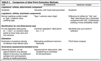
In theoretical work on spatial voting models, utility functions are usually deterministic and the precise functional form, aside from an assumption of quasi-concavity, is not specified. For empirical work, it is convenient to choose a parametric specification for the utilities and to add a stochastic disturbance. Several different specifications have been used, but all are quite similar. We assume a quadratic utility function for legislators with normal errors. Poole and Rosenthal (1997, 235–36) assume Gaussian utilities with extreme value errors. Heckman and Snyder (1997) assume quadratic utilities with uniform errors for one of the alternatives and nonstochastic utility for the other. See Table 2 for a comparison of the specifications.
The data consist of n legislators voting on m different roll calls. Each roll call j=1, …, m presents legislators i=1, …, n with a choice between a “Yea” position ζj and a “Nay” position ψj, locations in
, where d denotes the dimension of the policy space. Let yij=1 if legislator i votes Yea on the jth roll call and yij=0 otherwise. Legislators are assumed to have quadratic utility functions over the policy space,
, and
, where
is the ideal point of legislator i, ηij and νij are the errors or stochastic elements of utility, and ||·|| is the Euclidean norm. Utility maximization implies that yij=1 if
and yij=0 otherwise. The specification is completed by assigning a distribution to the errors. We assume that the errors ηij and νij have a joint normal distribution with E(ηij)=E(νij), var(ηij−νij)=σ2j and the errors are independent across both legislators and roll calls. It follows that
where
, and
denotes the standard normal distribution function. This corresponds to a probit model with an unobserved regressor xi corresponding to the legislator's ideal point (a logit model results if the errors have extreme value distributions). The coefficient vector βj is the direction of the jth proposal in the policy space relative to the Nay position.
Given the assumptions of independence across legislators and roll calls, the likelihood is
where B is an m×d matrix with jth row
,
, X is an n×d matrix with ith row x′j, and Y is the n×m matrix of observed votes with (i, j)th element yij.
The model, as described above, is the simplest possible form and is a convenient starting point for more elaborate models. For instance, we show later how it is possible to add party effects to this specification. Clinton and Mierowitz (2001) modify this framework to study agenda dependence. It is also possible to incorporate vote trading and cue-taking into the model by making the utility of one legislator dependent upon either the utility or the voting behavior of another.
The spatial voting model is equivalent to the two-parameter item response model used in educational testing,2
This equivalence has been noted by several authors, including Bailey and Rivers (1997), Londregan (2000a), and Poole and Rosenthal (1997, 247).
where
is the item discrimination parameter and
is the item difficulty parameter, but in the roll call context the latent trait or “ability” parameter xi is the ideal point of the ith legislator. There is a large literature in psychometrics on estimation of these models (e.g., Baker 1992 and Bock and Aitken 1981), but the focus is usually on estimation of the
(the item parameters), which are used for test equating. In roll call analysis, however, primary interest almost always centers on the xi (the ideal points), while in psychometrics the xj (ability parameters) are usually treated as random effects.
Identification
As it stands, model (2) is not identified. For example, suppose that we transform the matrix of ideal points X by premultiplying by an invertible d×d matrix R and apply the inverse transformation to the direction vectors B, X*=XR and B*=BR−1. Then the likelihood
for all possible voting patterns Y: no data can distinguish between the different parameter values because any translation or rotation of the ideal points and proposals leaves the distances between ideal points and alternatives unchanged.
Identification is essential for standard methods of estimation, such as maximum likelihood, which are inconsistent when the model is unidentified. The role of identification in Bayesian estimation is more controversial. Bayesian procedures can be applied to unidentified models, though the data are only informative about identified parameters (e.g., Neath and Samaniego 1997). However, in many cases it is difficult to formulate a reasonable prior for problems involving arbitrary rescalings. For example, we may have some prior information about tomorrow's temperature, but it is very difficult to quantify this information unless we agree in advance whether temperature is measured on the Fahrenheit, the celsius, or some other scale. This is a simple example of normalization. The same problem occurs in policy spaces since both the origin and the metric are arbitrary.
Rivers (2003) derives necessary and sufficient conditions for identification of multidimensional spatial models based upon a priori restrictions on the ideal point matrix X. In the case of a unidimensional policy space, the identifying conditions are straightforward: Two linearly independent restrictions on the ideal point matrix X are required. One possibility is to constrain the positions of two legislators at arbitrary positions, e.g., Kennedy at −1 and Helms at +1. Alternatively, we can constrain the ideal points to have mean zero and standard deviation one across legislators. This is sufficient for local, but not global, identification (since the left–right direction can be reversed by reflecting the ideal points around the origin and reversing the policy directions).
In d-dimensional choice spaces, d(d+1) linearly independent a priori restrictions on the ideal points X are required for identification. Thus, in two dimensions, it is necessary to fix the positions of three legislators (three ideal points, each with two elements). In general, local identification can be achieved by fixing the positions of d+1 legislators. Estimation becomes progressively more difficult in higher dimensions. In addition to the necessary identifying restrictions, it is also beneficial to add other a priori information (see Jackman 2001 for an example).
ESTIMATION AND INFERENCE
The classical or frequentist approach treats ideal points as fixed but unknown parameters. An estimation technique, such as maximum likelihood, is evaluated by considering its sampling distribution. We imagine the ideal points and other parameters to be fixed and draw repeated samples from the same data generating process. Each of these samples is a hypothetical roll call governed by the same ideal points and bill parameters. Because voting is probabilistic (see equation [1]), each sample yields different votes and hence different estimates of the ideal points and other parameters. The sampling distribution of an estimated ideal point is its distribution across a set of hypothetical roll calls.
The Bayesian approach, in contrast, treats the unknown ideal points and other parameters as random variables and conditions upon the observed roll call data. We represent any a priori information by a prior distribution over the parameters. Bayes' formula describes how to combine the prior information with the observed data to obtain a posterior distribution which summarizes our information about the parameters having seen the roll call data. The Bayesian approach, as we will see, allows us to make probability statements, such as “Kennedy is more likely than O'Connor to be the median justice on the Supreme Court.” Of course, this kind of statement is meaningless from the frequentist perspective, which treats the ideal points as fixed.
Bayesian methods are often thought of primarily as a way to use nonsample information in estimation. (See Western and Jackman 1994 for some examples from political science.) Our motivation for using Bayesian methods in roll call analysis, however, is rather different. Roll call data sets are usually very large, so in most cases the benefit to introducing additional a priori information is slight. Instead, the real benefit to the Bayesian approach is that it turns a very difficult classical estimation problem into a fairly routine application of Markov chain Monte Carlo (MCMC) simulation. Moreover, the Bayesian approach lets us make inferences about ideal points and substantive hypotheses that were intractable with classical techniques. And in addition, the Bayesian model and estimation procedures are easily extended to handle more complex formulations.
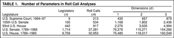
To understand better the computational challenge that roll call analysis presents for classical estimation, consider the number of parameters that need to be estimated in some typical applications. With data from n legislators voting on m roll calls, a d-dimensional spatial voting model gives rise to a statistical model with p=nd+m(d+1) parameters. Table 1 presents values of p for five different data sets. A moderately sized roll call data set (say the 105th U.S. Senate) with n=100, m=534 nonunanimous roll calls, and d=1 yields p=1,168 unknown parameters, while a two-dimensional model has p=1,802 parameters. A typical House of Representatives (e.g., the 93rd House) set has n=442 and m=917, so a one-dimensional model has p=2,276 parameters, while a two-dimensional model has p=3,635 parameters. Pooling across years dramatically increases the number of parameters: For instance, Poole and Rosenthal (1997) report that fitting a two-dimensional model to roughly 200 years of U.S. House of Representatives roll call data gave rise to an optimization problem with p>150,000 parameters.
The proliferation of parameters causes several problems. The usual optimality properties of conventional estimators, such as maximum likelihood, may not hold when, as in this case, the number of parameters is a function of the sample size (see Lancaster 2000 for a recent survey). In particular, the customary asymptotic standard error calculations, using the inverse of the information matrix, are not valid. As a practical matter, the size of the information matrix is too large for direct inversion. Poole and Rosenthal (1997, 246) take the obvious shortcut of fixing the bill parameters at their estimated values before calculating standard errors for the ideal point estimates. They point out that this is invalid, but it reduces the computational burden by an order of magnitude.
The Bayesian methods of estimation and inference proposed here are valid for finite samples and do not rely any large sample approximations. The number of parameters is fixed for any particular estimation problem by the actual number of legislators and roll calls and Bayes' theorem gives the posterior distribution of the parameters conditional upon the observed data. The only approximation involved is the simulation of the posterior distribution and this approximation can be made to any desired degree of accuracy by increasing the number of simulations (n.b., not the sample size, which is fixed for any given data set).
Details of the Bayesian simulation procedure we adopt are provided in the Appendix, but a brief heuristic explanation may be useful. The fundamental difficulty in roll call analysis is that everything other than the votes is unobservable: The ideal points, bill parameters, and utilities are unknowns. But if it were possible to impute values to the bill parameters and utilities, then the ideal points could be estimated by regression. By the same logic, if we were able to impute values for the ideal points and utilities, the bill parameters could also be estimated by regression. The MCMC algorithm repeatedly performs these imputations and regressions, starting from an arbitrary point and alternating between simulation of the ideal points, bill parameters, and utilities. Under a wide set of conditions (e.g., Tierney 1996) MCMC algorithms are guaranteed to generate samples from the posterior density of the model parameters, regardless of where in the parameter space the algorithm is initialized. In principle, MCMC algorithms are not hampered by the large number of parameters encountered in roll call analysis, although obviously computational time increases with the number of legislators and/or roll calls (see the Appendix) and monitoring the performance of the algorithm is more costly.
We use intentionally vague priors for most of the parameters. For each application below, we describe the actual prior used, but except where noted, the results appear to be insensitive to choice of prior.
COMPARISON WITH OTHER METHODS OF IDEAL POINT ESTIMATION
Having detailed our approach, Table 2 provides a summary of the differences between our approach, W-NOMINATE, and the factor-analytic approach of Heckman and Snyder. Our approach has more in common with W-NOMINATE than the Heckman–Snyder factor analysis approach. The Heckman–Snyder factor-analyic approach is distinctive in that the relatively simple statistical model (factor analysis) does not follow neatly from a formal model of legislative voting as our quadratic-probit model or the normal-logit model underlying W-NOMINATE3
The issue is that the Heckman–Snyder factor analytic statistical model results from a linear probability model for roll call voting, in turn driven by the assumption that the stochastic component of the legislators utility differential (the net utility a legislator has for voting Yea over voting Nay) follows a uniform distribution. In turn, the utility functions that rationalize this statistical model have unspecified stochastic components, since there does not exist a distribution such that the difference of two independent realizations from it yield a quantity with a uniform distribution. While no more ad hoc than the usual stochastic assumptions (normal or Type-1 extreme value errors), the H–S assumptions are somewhat idiosyncratic. This technical point aside, there are other more practical reasons to prefer our approach over factor-analytic approaches, such as the availability of standard errors and the extensibility of the model.
but provides ideal point estimates relatively cheaply; indeed, factor analysis supplies starting values for both the NOMINATE algorithms and our Bayesian simulation approach.
Example 1: 106th U.S. House of Representatives
To illustrate the differences and similarities between existing approaches and our simulation-based Bayesian estimator, we first analyze roll calls from the 106th U.S. House of Representatives via the several methods. We fit a one-dimensional model to these data using principal components (extremely similar to the Heckman–Snyder estimator),4
We implement the principal components estimator as follows: (1) compute an n×m matrix D by double-centering the roll call matrix, (2) compute P, an n×n correlation matrix (the correlation matrix of D′, using pairwise deletion of missing data), and (3) take the first d eigenvectors of P as the ideal point estimates for a d-dimensional model.
W-NOMINATE, as well as our Bayesian approach. We use the probit version of our model and impose the identifying constraint that the legislators' ideal points have mean zero and unit variance across legislators. After discarding lop-sided votes, W-NOMINATE uses 871 roll calls and does not fit an ideal point for Livingston (R-LA), who resigned from Congress in February 1999 after voting on 19 roll calls in the 106th House. Lop-sided votes and short voting records pose no problems in the Bayesian approach; we estimate ideal points for all legislators and include all but unanimous roll calls, yielding
m=1,073 roll calls in all, comprising 444,326 individual voting decisions. With predicted probabilities of .5 as a classification threshold we correctly classify 89.9% of the individual voting decisions
5 This classification rate is a function of the unknown model parameters and, so, is itself subject to uncertainty; here we report the classification rate averaging over uncertainty in the model parameters. See the discussion of auxiliary quantities of interest in section.
and find that 1,007 of the 1,073 (93.8%) roll calls discriminate with respect to the single latent dimension.
6 That is, these 1,007 roll calls all had slope coefficients (
, the equivalent of item discrimination parameters) whose 90% posterior confidence intervals did not cover zero.
Of the 66 roll calls that fail to discriminate with respect to the recovered dimension, only two roll calls were decided by margins closer than 60%–40%. In short, a one-dimensional model appears to be a very good characterization of these roll call data.
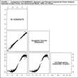
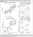
Figure 1 plots the three sets of ideal point estimates against one another. This figure exemplifies a pattern we have seen in many other roll call data sets: When n and m are both reasonably large and a low-dimensional model fits the data well, there is extremely little difference in the ideal point estimates produced by W-NOMINATE and our Bayesian estimator. In this specific example, n=440, m=1,073, and a one-dimensional model gives an extremely good fit to the data (as is typical of recent U.S. Congresses), and the ideal point estimates correlate at .996. Nonetheless, by retaining more of the lop-sided votes than W-NOMINATE, our Bayesian estimator can discriminate among extremist Democrat legislators (in the left tail), effectively “stretching” the distribution of the Democrats ideal points relative to W-NOMINATE's estimates. The comparison of both W-NOMINATE and our Bayesian estimator with the principal components estimator reveals the linearity of the factor analytic model, with the two nonlinear models both generating more discrimination among extremist legislators.
ESTIMATION AND INFERENCE FOR AUXILIARY QUANTITIES OF INTEREST
An advantage of the Bayesian approach is that it is straightforward to estimate posterior distributions over any auxiliary quantity of interest that is a function of the model parameters. These quantities of interest can be any function of the model parameters, as we now demonstrate.
Example 2: Pivotal Senators in the 106th U.S. Senate
The notion of pivotal legislators is critical to many theories of legislative behavior. For instance, supermajorities are often needed for extraordinary legislative action, such as the two-thirds majority required to override a presidential veto or the 60 votes needed to pass cloture motions in the U.S. Senate. Order statistics of ideal points play a prominent role in theories of legislative politics: e.g., the “gridlock interval” is defined as the region between the filibuster pivot and the veto pivot, and in the case of a liberal president the gridlock interval is bounded on the left by the veto pivot (the 33rd senator) and on the right by the filibuster pivot (the 60th senator) (e.g., see Krehbiel 1998, Fig. 2.2). Formal theories of legislative politics make sharp and exact predictions on the basis of these pivotal locations: e.g., proposals that attempt to change status quo policies located in the gridlock interval will not succeed. To operationalize these theoretical predictions, the gridlock interval is usually computed using the estimated ideal points of the corresponding legislators (e.g., Howell et al. 2000). Similarly, Schickler (2000) characterizes the parties' ideological positions with the ideal points of the median legislator within each party. Given the importance of individual legislators such as the chamber median or the “filibuster pivot” (i.e., the 40th senator), it is straightforward to generate posterior estimates for both the identity and the spatial location for such legislators in our Bayesian simulation approach.
Consider the task of uncovering the identity of the “pivotal” senators in the 106th Senate (n=102, m=596 nonunanimous roll calls; there are 102 senators because of the replacement of John Chafee (RI) by his son Lincoln Chafee and the replacement of Paul Coverdell (GA) by Zell Miller, although in assessing rank order we ignore the “replacement senators”). We fit a unidimensional model to these data, again with the identification constraint that the ideal points have mean zero, variance one across legislators. To determine which senators are critical for invoking cloture or which are the median senators requires recovering the posterior distribution of the rank of each senator's ideal point. We compute this by repeating the following scheme an arbitrarily large number of times: (1) sample the legislators' ideal points xi from their joint posterior density; (2) rank order the sampled ideal points; (3) note which legislator's occupies a particular pivot or order statistic of interest. We then report the proportion of times the ith legislator's ideal point is the pivot or order statistic of interest over these repeated samples from the posterior of the ideal points. Since we are working with an arbitrarily accurate approximation of the joint posterior density for the ideal points, inferences as to the ranks and the identity of the legislators occupying particular ranks are also arbitrarily accurate.7
In principle, one could implement a similar procedure with W-NOMINATE estimates, but two complications arise: (1) all covariances among ideal points are implicitly set to zero since W-NOMINATE only reports pointwise standard errors on each ideal point and (2) an asymptotically valid normal approximation is assumed to characterize ideal point uncertainty (less pressing when working with large roll call data sets). Lewis and Poole (2003) use parameteric bootstrapping.
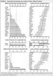
Figure 2 summarizes the posterior densities over the identities and locations of the senators at key pivot points. We omit the “replacement senators” Chafee and Miller from these calculation. There is almost no doubt as to identity of the chamber median: Republican Senators Snowe and Collins are the only senators with positive probability of being the 50th senator, with Collins overwhelmingly most likely to be the 50th (p=.98). Twenty-two senators have discernible probability of being the veto pivot (the 33rd senator), with 10 senators having probabilities greater than 5% of being the veto pivot: Senators Baucus (p=.12), Biden (p=.11), Johnson (p=.08), Graham (p=.08), Bayh (p=.08), and Cleland (p=.08) account for roughly half of the uncertainty as to the identity of the veto pivot, but clearly no one senator is unambiguosly the veto pivot. Thirteen Republican senators have positive probability of being the filibuster pivot (the 60th Senator), five of whom have p>.05, with Stevens the most likely candidate for the filibuster pivot (p=.41), followed by Warner (p=.26) and Campbell (p=.09).
A similar computation can be performed to recover the estimated spatial location of pivotal legislators. The right-hand panels in Figure 2 show the location of the median, veto pivot, and filibuster pivot (with confidence intervals), along with the estimated ideal points (posterior means) and 95% confidence intervals of adjacent senators. Again, it is apparent that there is little uncertainty as to the median (Senator Collins). But an interesting result arises for the veto pivot: Although we are unsure as to the identity of the veto pivot, we are quite sure as to the veto pivot's location. A similar result is also apparent for the filibuster pivot. While we may be able to pin down the location of either pivot with some precision, we do not know which legislators will be the veto and filibuster pivots on any given vote. This is a seldom noticed feature of contemporary U.S. Congresses, but one with implications for lobbying and legislative strategy; i.e., relatively precise knowledge of where the pivots lie does not correspond to knowing the identity of pivotal legislators, whose votes are necessary to guarantee cloture or veto-proof majorities.
Example 3: Party Switchers and the “Party Influence” Hypothesis
A major advantage of our modeling approach is the ability to extend the model to encompass alternative models of legislative behavior. For instance, thus far we assumed a Euclidean spatial voting model, in which, conditional on legislators' unobserved ideal points (which are considered constant over the period spanned by the roll call data), voting is independent across legislators and roll calls. In the next set of examples we consider alternatives to this basic setup, all of which are easily accommodated in our approach.
A question of particular interest to congressional scholars is the influence of political parties on the voting records of legislators. Party switchers—that is, legislators who change parties between elections, while continuing to represent the same geographic constituency—provide something akin to a natural experiment: The switcher's change in party affiliation helps identify a “party effect,” since many other determinants of roll call voting remain constant (e.g., characteristics of the legislators' constituency). The typical investigation of party switchers (e.g., Nokken 2000) uses a “pre/post” or “differences-in-differences” design, comparing changes in ideal point estimates for the party switcher relative to the changes among the switcher's fellow legislators or a random selection of nonswitchers (McCarty, Poole, and Rosenthal 2001).8
An obvious threat to this approach is self-selection into the “treatment” of party switching, say, if party switching is motivating by change in the personal preferences of the legislator; in this case we could not distinguish any party effect from an effect due to the personal preferences of the legislator, but we do not pursue this issue here. Other analyses of party switchers have also noted this problem: See McCarty, Poole, and Rosenthal (2001, 686).
By definition, splitting the roll call data into “pre” and “post” switching periods gives us fewer data than in the entire legislative session, and, as a consequence, ideal point estimates based on the pre and post sets of roll calls will be less precise than those based on all roll calls. Any comparison of change in the ideal points ought to properly acknowledge the relative imprecision arising from the smaller sets of roll calls available for analysis. A strength of our Bayesian simulation approach is that we routinely obtain uncertainty assessments for all model parameters, and all inferences will reflect the drop in precision occasioned by slicing the roll call matrix around the party switch.
The flexibility of our approach lets us formally embed a model for change in ideal points in a statistical model for roll call data, greatly facilitating investigation of the party switching hypothesis. Let
designate the party switcher and xi1 and xi0 be the ideal points of legislator i in the postswitch and preswitch periods, respectively. Then a weak form of the party switcher hypothesis is that
(i.e., the party switcher's ideal point changes, presumably in a direction consistent with the change in parties). A strict form of the party switcher hypothesis involves the n−1 additional restriction
, if i≠s (i.e., the party switcher is the only legislator whose preswitch and postswitch ideal points differ). An intermediate version of the switching hypothesis maintains that legislative ideal points may “drift” but that the party switcher's
is larger than the nonswitchers'
. In any event, we require estimates of each legislators'
, either by running two separate analyses (splitting the roll call data around the time of the party switch) or by a more direct (but equivalent) approach in which we parameterize the postswitch ideal points as
.
Since the pre- and post-switch roll calls do not refer to identical proposal and status quo positions, some normalization is required to compare the resulting ideal point estimates. Our solution is to focus on relative changes, since without further assumptions, any “global” or “uniform” shift in the legislative agenda or preferences around the party switch is unidentified. That is, the average postswitch legislative proposal may be more liberal than the average preswitch proposal by distance
, or (observationally equivalent) all legislators may move
to the right (put simply, there is no guarantee that the pre and post ideal point estimates are comparable). Solutions to this scaling problem abound: One could try to find bills with identical “Yea” and “Nay” locations in both periods, or assert that particular legislators do not move across the party switch. The identifying restriction we adopt is to estimate subject to the constraint that the legislators' ideal points have mean zero and unit variance in each period and that we interpret the
as relative changes.
We illustrate our method with the 107th U.S. Senate. On May 24, 2001, Senator James M. Jeffords (VT) announced that he would leave the Republican party and become an independent. The switch was particularly consequential, giving the Democrats control of the Senate: The postswitch partisan composition was 50 Democrats, 49 Republicans, and 1 Independent (Jeffords). One hundred forty-eight nonunanimous votes were recorded in the 107th Senate prior to Jeffords's switch, and 349 were recorded post-switch.
Figure 3 summarizes the preswitch and postswitch ideal point estimates (top panels) and rank orderings (lower panels). We find that the ideal points underlying Jeffords' voting behavior differ across the switch: The estimate of Jeffords's postswitch ideal point is statistically distinguishable and more liberal than the preswitch estimate, indicating that a shift in Jeffords's preferred policy position accompanied his switch in party affiliation.
But of course, there are numerous other senators who do not switch parties but whose ideal points do move markedly. Points above (below) the 45° lines in the left-hand panels in Figure 3 indicate senators moving in a conservative (liberal) direction. The 10 largest changers in terms of ideal points are presented in the top-right panel; the 10 largest changers in terms of rank order appear in the lower-right panel (horizontal bars indicate 95% confidence intervals). The largest changer in terms of spatial location is Wellstone (D, MN), with a jump to the left estimated to be about .75 on the recovered scale. Since Wellstone is a preference outlier, his ideal points (and hence change in ideal point) are estimated with considerable imprecision. Jeffords's change is almost as large, but estimated with considerably more precision. However, even after taking into account uncertainty in the magnitude of the changes, there is no disputing that Wellstone's change is larger: The probability that Wellstone's change is the largest change is .284, while the probability that Jefford's change is the largest is only .068.9
The probability that Senator X is the biggest changer is computed as the proportion of times a particular senator's change is the largest change, over many draws from the posterior density of the preswitch and postswitch ideal points (i.e., we induce a posterior density on the identity of the largest switcher. This example again highlights the flexibility and ease of the Bayesian simulation approach to estimation and inference for roll call analysis. See also the earlier example where we induce posterior densities over the identity of critical pivots.
Intriguingly, other large changers in terms of spatial location are the two party leaders, Daschle (D, SD) and Lott (R, MS). With Jeffords leaving the Republicans, Daschle becomes majority leader while Lott becomes minority leader. Both Daschle and Lott move in a conservative direction, and are the third and fifth largest changers, respectively. When we trun to a consideration of ranks (lower panels in Figure 3; Daschle is the largest switcher, moving 31 places to the right and becoming markedly more moderate relative to other senators. Daschle changes from about the 10th senator (95% bound: 2nd–21st) to the 41st (35th–45th) senator (arraying senators from left to right, or liberal to conservative), jumping from being unambiguously on one side of the Democratic senate median to the other. Lott is the fourth largest changer in terms of ranks (20 places), jumping from the 77th senator (68th–87th) to the 97th (95th–100th). Jeffords, the party switcher, is only the seventh largest switcher in terms of ranks and is the largest switcher with probability .01. Daschle is the largest switcher in terms of rank, with probability .786. We would reject any hypothesis that the party switcher's change was the largest change we observe, in terms of either spatial location or ranks.
These results are based on a unidimensional fit to a single congress, and, fortuitously, a party switch that brought about a change in party control of the Senate, and so we are cautious about reaching for any broad conclusion. Nonetheless, these results are consistent with policy moderation by majority leaders, perhaps in order to more effectively represent and articulate party policy positions, or even so as to secure the majority leadership in the first instance.
This example models change in ideal points around a recent, vivid instance of party switching. But other models of change in ideal points can be easily fit into this framework. Party switchers perhaps provide the most direct evidence of party effects, but the methodology can be used to examine changes elsewhere (e.g., across congressional sessions, congresses, or politically consequential “shocks” in American political history).
Example 4: A Two-Cutpoint, “Party Influence” Model
Our final example again examines the question of party pressure in legislative behavior. The standard model assumes that conditional on a legislator's ideal point xi and the vote parameters
, vote yij is independent of yi′j′, for all i≠i′, j≠j′: e.g., shocks making legislator i more likely to vote Yea do not make legislator i′ any more or less likely to vote Yea. Accordingly, the recovered ideal points need to be interpreted with some caution. Party influence or “whipping” is one way that conditional independence can be breached: e.g., legislators whose preferences might lead them to vote Yea are persuaded to vote Nay, and vice versa. Modeling roll call data without considering these possibilities leads to ideal point estimates that absorb a shock common to members of a given party (or, say, a whipped subset of a party's members); to the extent that party influence is an unmodeled common shock, then the recovered xi display greater partisan polarization than exists in the “true” xi. Note that while party influence is a plausible mechanism for generating party-specific utility shocks, we are wary of inferring the presence of party pressure given evidence of party-specific utility shocks; we acknowledge that other mechanisms may generate party-specific utility shocks (e.g., lobbying by activists or interest groups that targets legislators from one party more than the other) and so we refer to “party-specific inducements” rather than “party-pressure.”
It is straightforward to augment the standard voting model to allow for party-specific inducements. For instance, suppose that in addition to the standard quadratic spatial utilities, legislator i receives
, a net incentive to vote Yea vis-à-vis Nay on vote j, but where the net incentive is specific to i's party affiliation, Pi=D if i is a Democrat and Pi=R if i is a Republican. If there are only two parties, then
and
are unidentified. At best we can estimate a net difference in party-specific inducements,
(see also Krehbiel 2003): i.e., we estimate y*ij≡Uij(“Yea”)−Uij(“Nay”)
, where Di is a binary indicator coded one if legislator i is a Democrat and zero otherwise, and for this example we assume that the
are iid logistic (logit rather than probit).10
McCarty, Poole, and Rosenthal (2001) refer to this class of model as a “two-cutpoint” model, since it implies separate points where legislators of each party are indifferent between voting “Yea” and voting “Nay.”
Since the standard model nests as a special case of the two-cutpoint model, it is straightforward to assess whether the restrictions implicit in the standard model are valid, by testing the joint null hypothesis
H0:
, for all j.
In addition, we also need to define a set of votes in which the net party-specific inducements are not relevant (or can be reasonably assumed to be zero), since if every roll call was assumed to be potentially subject to party influence, then there is no way to compare the recovered ideal points of Democrats and Republicans. By way of analogy, consider standardized test items that (say, due to cultural biases) are suspected to be easier for group A than for group B: a phenomenon known as differential item functioning (DIF); e.g., see Holland and Wainer (1993). Does better test performance by group A reflect higher ability than group B, or DIF? Unless we can identify a set of test items that are known to be DIF-free and use these items to pin down ability, then there is no way to distinguish apparent differences in ability from DIF.
Several implementations of party influence models appear in the literature. Snyder and Groseclose (2000) use a two-stage procedure: First, using lop-sided votes (those decided by more than 65/35 margins), estimate xi via the standard model using the linear factor-analysis model due to Heckman and Snyder (1997); second, on non-lop-sided votes, estimate the linear regression of votes on xi and a dummy variable for Democratic legislators, with the coefficient on the dummy variable interpreted as a coefficient of party influence. Aside from (1) equating net party-specific inducements with party influence and (2) assuming no net party-specific inducements for lop-sided votes, this approach makes some strong additional assumptions: (3) the use of the Heckman–Snyder factor-analytic estimator in the first stage; (4) the use of a linear regression model with the binary dependent variables (Yeas and Nays) in the second stage (Synder and Groseclose use a Huber–White robust variance–covariance estimator to correct for the resulting heteroskedasticity); and (5) the fact that the xi result from a measurement procedure (the first stage) and generate an “errors-in-variables” problem, which Synder and Groseclose tackle via instrumental variables.11
Another implementation of the two-cutpoint approach appears in McCarty, Poole, and Rosenthal (2001), using a nonparametric optimal classification algorithm (Poole 2000): they compare the increase in classification success in moving from one to two cutpoints.
In contrast, our approach provides a direct way to test for party influence; our modeling approach is easily extended to let us embed parameters tapping party influence. That is, we fit one model to the data, with the statistical specification following directly from augmenting the utility functions with inducements specific to each vote, by party affiliation. In this way there is no need to break the estimation into separate pieces (one to recover ideal point estimates free of party effects, the other to recover estimates of effects, conditional on the ideal points recovered from the first stage): Uncertainty in the recovered ideal points estimates propagates into uncertainty in the estimates of the vote-specific parameters (
,
, and
), and vice versa. The two-stage approach has been criticized for generating baised estimates of the ideal points of moderate legislators in the first stage (e.g., McCarty, Poole, and Rosenthal 2001, 675–77). But with our approach we use all votes to learn about the legislators' ideal points—even those votes thought to be subject to party pressure—and so we are less prone to this source of bias.
Note that in our parameterization the
are net utility shocks specific to Democratic senators and, so, alternate sign depending on whether the net party-specific inducement was for Democrats to vote Yea (
) or Nay (
). In addition, for perfect party line votes, the likelihood for the data attains a maximum at
(i.e. votes with perfect separation by party are consistent with an infinite amount of party pressure!), causing classical estimation procedures to break down. Party pressure may be large or small, but certainty not infinite, and we express this belief via proper prior densities on the
that assign infinitesimal probability to infinite party pressure, and bound the posterior densities for
away from ±∞.12
Note that Snyder and Groseclose (2000) effectively sidestep this issue by fitting the binary roll data by least-squares linear regression.
We estimate our expanded model with 534 nonunanimous roll calls from the 105th U.S. Senate (55 Republicans, 45 Democrats). To identify the model we constrain Senators Kennedy and Helms to have ideal points of −1 and 1, respectively. The two-cutpoint model requires the additional identifying constraint
among roll calls decided with majorities of 65% or more (“lop-sided” votes), consistent with the Snyder and Groseclose (2000) approach: 257 of the 534 nonunanimous roll calls meet this criteria. Vague normals prior distributions are used for the
parameters (mean zero, variance 16) for the remaining 277 “close” roll calls (decided by margins closer than 65–35). Of these close roll calls, 93 (33.6%) have net party-specific inducements that are significantly different from zero (again, in the sense that the 95% confidence interval on the corresponding
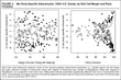
does not overlap zero). Figure 4 plots the means of the posterior density of each
parameter against the margin of victory (left panel) and party cohesion (right panel) per “close” roll call. Our analysis shows that net party-specific inducements are at their largest for roll calls decided along party lines and decline as the votes become more lop-sided. Nonetheless, the extent of party line voting we find here is smaller than those reported by Snyder and Groseclose (2000) and closer to the proportions found by Cox and Poole (2002), although the latter analysis considered voting in the House of Representatives.
The actual magnitudes of the
warrant elaboration as well. The smallest, statistically significant
we obtain are roughly ±2.0. To assess the magnitude of this effect, consider a moderate Republican and Democrat who ex ante are indifferent between voting Yea and voting Nay. A net party-specific inducement corresponding to
makes the probability of the Democrat voting Yea about .73 and the corresponding probability for the Republican .27. If the net party pressure is all one-sided, say all Democratic, then the probability of the Democrat voting Yea goes up to .88; conversely, if the party pressure is all Republican, then the probability of the Republican voting Yea is .12. Note that these are the smallest statistically significant estimates of
we obtain, with estimates of ±4 being more common. That is, although we find evidence consistent with party pressure on just one-third of close votes, the magnitude of that pressure seems large and politically consequential.
We can compare the ideal point estimates produced by our augmented model with those from the standard model. A standard one-dimensional spatial voting model finds absolutely no overlap between the ideal points of Democrats and Republicans in the 105th U.S. Senate. This complete separation between the parties arises in part because any voting on close votes driven by party-specific inducements is attributed wholly to differences in the legislators' ideal points. Once we admit the possibility of party-specific inducements, the two partisan groupings actually overlap: Breaux, the most conservative Democrat, has roughly the same ideal point as the most liberal Republicans, Specter and Jeffords. Even after estimating net party-specific inducements specific to each roll call, we still find considerable partisan polarization but substantially less polarization than the levels recovered from a conventional statistical analysis using the standard model.
CONCLUSION
Roll call analysis and the statistical operationalization of the Euclidean spatial voting model is a critical component of the scientific study of legislative politics. Although existing methods for the statistical analysis of roll call data have been employed in many settings and produced important insights, the Bayesian simulation approach we present builds upon and improves extant methods in several ways. First, Bayesian methods permit auxiliary information to be brought to bear on roll call analysis in a straightforward and theoretically consistent way; this auxiliary information may include (but is not restricted to) expert judgments about dimensional structure, the location of extremist legislators, legislator-specific covariates, or the evolution of the legislative agenda. Second, the methodology we present is sufficiently flexible so as to easily accommodate alternative models of legislative behavior. For example, it is possible to permit ideal point estimates to change over time by modeling the process associated with that change (e.g., legislators switching affiliations between political parties). Finally, Bayesian simulation exploits tremendous increases in computing power available to social scientists over the last decade or so: Estimation and inference via simulation—long known to be an attractive statistical methodology (e.g., Metropolis and Ulam 1949)—is now a reality. Consequently, our model works in any legislative setting, irrespective of the size of the legislature or its agenda.
Thus Bayesian methods can make roll call analysis less a mechanical scaling exercise in which scholars simply feed roll call data to a “black box” algorithm and more a way to test theoretically interesting models of legislative behavior. In sum, the Bayesian simulation methodology we present lets scholars (1) incorporate substantive information about the proposals being voted upon or (2) about the prefenences that structure the ideal points being estimated, (3) impose theoretically implied constraints on the standard model, and (4) easily estimate and test alternative and models of legislator voting.
APPENDIX
Markov Chain Monte Carlo Algorithm
The difference between the utilities of the alternatives on the jth roll call for the ith legislator is
, where, for simplicity, we have set σj=1. If
and
are given, then xi is a vector of “regression coefficients” that can be imputed from the regression of
on
using the m votes of legislator i. If xi is given, then we use the votes of the n legislators on roll call j to impute
and
. Then given xi,
, and
, the latent utility differences y*ij are simulated by drawing errors from a normal distribution subject to the constraints implied by the actual votes (if yij=1, then y*ij>0, and if yij=0, then y*ij<0), and the process repeats.
In our Bayesian approach, priors are required for all parameters:
and
, j=1, …, m and xi, i=1, …, n. For the probit version of our model we have standard normal errors
and normal priors for the ideal points and the
and
parameters, leading to simple expressions for the conditional densities that drive the MCMC algorithm. For
and
, we denote the priors
); we generally choose vague priors by setting
and
, with
a large positive quantity (e.g.,
). For the legislators' ideal points, we use the normal prior
, where usually vi=0 and Vi=Id (an identity matrix of order d), but for legislators we are fixing to an set location (e.g., Kennedy and Helms, so as to normalize the scale of the latent traits), we use the prior
, where
is an arbitrarily small, positive quantity (i.e., a “spike prior” at xi).
The goal is to compute the joint posterior density for all model parameters
and
and xi, i=1, …, n. A MCMC algorithm provides a computer-intensive exploration or “random tour” of this joint density, by successively sampling from the conditional densities that together characterize the joint density. The model here is isomorphic with a two-parameter item–response theory model: Albert (1992) showed how an MCMC algorithm can be used to explore the posterior density of this model; see also Patz and Junker (1999) and Johnson and Albert (1999). Augmenting the MCMC algorithm with the latent y*ij greatly simplifies the computation of the probit version of the model, letting us exploit standard results on the Bayesian analysis of linear regression models as we show below; we obtain y*ij by sampling from its predictive density given the current values of the other parameters and the roll call data. Letting t index iterations of the MCMC algorithm, iteration t of the algorithm comprises sampling from the following conditional densities.
- . At the start of iteration t, we have , and x(t−1)i. We sample y*(t)ij from one of the two following densities, depending on whether we observed a Yea (yij=1) or a Nay (yij=0):
(truncated normal),
(truncated normal),
where and I(·) is an indicator function. For abstentions and other missing roll calls we sample y*(t)ij from the untruncated normal density , effectively generating multiple imputations for these missing data over iterations of the MCMC algorithm.
- . For j=1, …, m, sample and from the multivariate normal density with mean vector and variance–covariance matrix [X*′X*+T−10]−1, where X* is an n×(d+1) matrix with typical row x*i=(x(t−1)i, −1), y*(t)j is an n×−1 vector of sampled latent utility differentials for the jth roll call, and recalling that is the prior for and . This amounts to running “Bayesian regression” of y*(t)j on x(t−1)i and a negative intercept and then sampling from the posterior density for the coefficients and , for j=1, …, m.
- . Rearranging the latent linear regression yields . Collapse these equations over the j subscript, to yield the n regressions , where B is the m×d matrix with the jth row given by . That is, we have n regressions, with the ideal points xi as parameters to be updated. Again exploiting conjugacy, the update is performed by sampling each x(t)i from the d-dimensional normal density with mean vector (B′B+V−1i)−1(B′wj+V−1ivi) and variance–covariance matrix (B′B+V−1j)−1. After updating all xi(i=1, …, n), we optionally renormalize the xi to have zero mean and unit variance, say, when fitting a unidimensional model without a Kennedy-Helms type restriction.
Sampling from these distributions updates all the unknown quantities in the probit model. At the end of iteration t, denote the current values of the parameters of interest as
. Iterating the MCMC algorithm produces a sequence
, \ldots that comprises a Markov chain, with the joint posterior density for
as its limiting distribution. That is, after a large number of iterations of the algorithm, successive samples of
are drawn from its posterior density. These samples are saved and summarized for inference. Any function of these parameters can also be computed and saved, such as rank orderings of the legislators, pairwise comparisons of legislators, or the separating hyperplanes for particular roll calls.
The MCMC algorithm is initialized as follows. For the ideal points, we perform the eigen-decomposition described in footnote 4. These initial values are the estimates we would get from treating the ideal-point estimation problem as a principal-components factor analysis problem, ignoring the fact that the roll call data are not continuous variables (the binary character of the roll call data becomes less problematic as m→∞, and so for large roll call data sets from contemporary U.S. Congresses this procedure yields excellent start values). We are grateful to Keith Poole for suggesting this procedure, which is also used to generate start values for NOMINATE. For the bill-specific parameters
and
we obtain start values by running probits of the observed votes yj on the start values for the ideal points, j=1, …, m.
With any MCMC approach, diagnosing convergence of the Markov chain is critical. Our experience is that the MCMC algorithm performs reasonably well for the roll call problem, moving away from start values to the neighborhood of a posterior mode quite quickly. For simple unidimensional fits, we usually let the sampler run for anywhere between 50,000 and 500,000 iterations and then thin the output (storing the output of every 100th to every 1,000th iteration) so as to produce a reasonable number of approximately independent samples from the posterior for inference (say, between 250 and 1,000 samples).
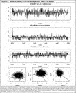
Figure 5 shows trace plots of the MCMC algorithm for single parameters (the ideal points of Kennedy, Collins, and Helms, from a unidimensional model fit to 106th U.S. Senate) in the top three panels and for the joint density of selected pairs of legislative ideal points in the lower panels. The identifying restriction is that the ideal points have mean zero and variance one across legislators. In the upper panels, the MCMC algorithm is approximately a random walk without drift in the parameter space, consistent with the sampler behaving well, randomly traversing the posterior density; the gray line indicates the posterior mean based on the post “burn-in” samples, and the dotted lines indicate 95% confidence intervals. The snaking solid lines are smoothed or moving averages and a cumulative mean; note that after sufficient iterations, the cumulative mean of the MCMC algorithm becomes indistinguishable from the posterior mean, and the running mean slowly undulates about the posterior mean, indicating lack of drift (consistent with the sampler having converged on the posterior density). Half a million iterations were computed; so to as produce approximately independent samples from the posterior density, only every 1,000th iteration is retained for making inferences and the thinned iterations have AR(1) parameters averaging about .06 (maximum AR[1]=.23, for Boxer). In the lower panels, each joint posterior mean is indicated by an open circle, and joint 95% confidence intervals are indicated by ellipses, the latter computed assuming that the joint posterior densities can be approximated with bivariate normal densities.
Computing
For small roll call data sets, the free, general-purpose MCMC package WinBUGS (Spiegelhalter et al. 1997) can be used to implement our approach: only a few lines of WinBUGS commands are needed. For instance, the WinBUGS code for a simple unidimensional model fitted via logit and the Kennedy–Helms identification constraint is given in Table 3. Elaborations on this basic setup are available at Jackman's Web site (http://jackman.stanford.edu/ideal). Given the computational burden of analyzing larger roll call data sets, we use a C program, authored by Jackman, implementing the MCMC algorithm for the probit model discussed above. In turn, this program can be called directly from the (free) R statistical program. We also use R for preparing roll call data sets for analysis, inspecting the output of the MCMC algorithm, and producing the graphs and tables in the body of the paper. All code is available upon request.
Computing time is clearly a relevant consideration for simulation-based methods. Our experience is that computing time increases in nmT, where n is the number of legislators and m is the number of bills, and so nm is the number of individual voting decisions being modeled (assuming no abstentions or missing data), and T is the number of MCMC iterations desired. The computational cost of moving to higher dimensions is surprisingly small. The unidimensional 106th U.S. Senate example involved modeling n=102 ideal points and m=596 pairs of bill (or item) parameters, with 58,156 nonmissing individual voting decisions. Half a million iterations of the MCMC algorithm required just over three hours on a Dell PC with a 3.0 GHz Intel processor, or about 2,650 iterations per minute. For a one-dimensional fit to the 106th House (n=440, m=1,073, with 444,326 nonmissing individual voting decisions), a 150,000-iteration run took 6.4 h, or about 391 iterations per minute, on the same hardware. For a one-dimensional fit to the U.S. Supreme Court (n=9, m=213, with 1,907 nonmissing individual voting decisions), a 500,000-iteration run took 15 min, or about 33,250 iterations per minute. These extremely long runs are usually not necessary, but we were being especially cautious about ensuring that the MCMC algorithm had converged on and thoroughly explored the posterior density.
We thank Larry Bartels, David Brady, Richard Brody, Jim Fearon, John Ferejohn, Rui de Figueiredo, Tim Groseclose, Keith Krehbeil, Jeff Lewis, John Londregan, Adam Meriowitz, Keith Poole, David Primo, and Mike Tomz for useful comments.






Comments
No Comments have been published for this article.