Previous work

Investigations of the role of basal till deformation in glacier dynamics have been carried out on glaciers such as Trapridge Glacier, Canada, Storglaciären, Sweden, and on Ice Stream B, Antarctica. Reference Hooke, Hanson, Iverson, Jansson and FischerHooke and others (1997) and Reference Fischer, Clarke and BlatterFischer and others(1999) found that the coupling of ice and till becomes weaker during times of higher basal motion, but we have not found any evidence for this beneath Black Rapids Glacier, Alaska, U.S.A. (Reference Truffer, Harrison and EchelmeyerTruffer and others, 2000). The motion across the ice/till interface on this glacier could have been, at most, a small fraction of the required 30–40 m of annual basal motion.

In contrast to differential motion at the ice/till interface, several modeling studies have assumed that basal till is deforming viscously (see Reference PatersonPaterson, 1994, for references), following the work of Reference Boulton and HindmarshBoulton and Hindmarsh (1987) and Reference Boulton and DobbieBoulton and Dobbie (1998). However, there is little other direct experimental or observational evidence to support such a rheology. Deformation studies on small samples indicate that, instead, a Coulomb-plastic rheology is more applicable (Reference KambKamb, 1991; Reference Iverson, Hooyer and BakerIverson and others, 1998; Reference Tulaczyk, Kamb and EngelhardtTulaczyk and others, 2000). These latter authors also offer some explanations of the observed distributed deformation profiles in terms of an elastic–plastic till model. Reference ClarkeClarke (1987) developed a framework to describe till in the context of soil mechanics, which usually incorporate these plastic rheologies. Our observations beneath Black Rapids Glacier support these latter studies, and provide additional evidence that, at least in some cases, till does not follow a viscous rheology (Reference Truffer, Harrison and EchelmeyerTruffer and others, 2000). In the present paper we use a perfectly plastic rheology for till, consistent with our direct observations. We therefore assume that there is no till deformation if the basal shear stress is below the failure strength of the till, and that the strength of the till is independent of the deformation rate.

A spectrum of basal conditions, ranging from a several-meter-thick till layer to a relatively clean ice/bedrock interface, is probably encountered in Nature. Many of the observations discussed in this paper have previously been discussed in the context of a clean ice/bedrock interface. Here we address the other end of the spectrum, and explore such a model in the context of glacier motion and hydrology.

Black Rapids Glacier

Black Rapids Glacier is a 40 km long glacier in the central Alaska Range; it is a surge-type glacier that is presently in its quiescent phase. It has been investigated in detail since 1973 (see, e.g., Reference Heinrichs, Mayo, Echelmeyer and HarrisonHeinrichs and others, 1996). A recent drilling program has revealed a 5–7 m thick basal till layer, and a seismic study (Reference Nolan and EchelmeyerNolan and Echelmeyer, 1999a, b) suggested that the till is at least locally abundant, with a signature at least 40 000 m² in extent. This latter study also found that the seismic properties of the entire till layer can change rapidly. A till-deformation study (Reference Truffer, Harrison and EchelmeyerTruffer and others, 2000) showed that most of the measured surface motion occurs at the bed, and that this basal motion occurs at a depth of > 2 m below the ice/till interface. Recent observations also include high-resolution (4 d⁻¹) global positioning system (GPS) measurements of surface velocity and vertical motion at three sites on the glacier. Figure 1 shows a map of the glacier and the location of the boreholes where most of these studies have been undertaken and where large velocity variations have been observed. The names of the boreholes are, from north to south: N1, Center and S1. The depth at the center of the channel is 620 m.

Fig. 1.

Map of Black Rapids Glacier. The diamonds show the positions of the drillholes. A dot marks every 5 km starting from the head of the glacier. The dashed line shows the Denali Fault. Units are meters in a local coordinate system.

Boundary conditions

The shear strength τ _s of a till layer along the transverse perimeter of the glacier channel is related to the effective pressure through a Coulomb failure criterion:

where φ is the angle of internal friction and c _a is the apparent cohesion. The effective pressure is the difference between the overburden p _o and the pore-water pressure p _w. The pore-water pressure depends on the water pressure at the ice/till interface and changes within the till, as discussed below. We make the approximate assumption that the pore-water pressure is not affected by till deformation (Reference Iverson, Hooyer and BakerIverson and others, 1998).

The name “apparent cohesion” for c _a results from the observation that Equation (1) is not strictly valid near zero effective pressure, at which point the shear strength of a granular material is actually zero (Reference WoodWood, 1990). The apparent cohesion is usually a negligible quantity; on one sample from Black Rapids Glacier we measured 1.3 kPa (Reference Truffer, Harrison and EchelmeyerTruffer and others, 2000). Here we take it to be zero.

Equation (1) defines a relationship between the shear strength and the effective pressure. The material properties of the till are determined by the friction angle φ (and the cohesion). In the remainder of this paper we will call a till “stronger” or “weaker” if its shear strength changes as a result of changes in effective pressure; no change in material properties (i.e. φ) is implied with this terminology.

The distribution of basal water pressure is needed to calculate the effective pressure at the glacier bed, and therefore the till strength. Water pressures along the glacier bed are determined by the nature of the subglacial drainage system. Reference Walder and FowlerWalder and Fowler (1994) proposed that water drains through shallow “canals” in the till. They obtained a direct relationship between water flux and pressure which favors a distributed drainage system. This relationship, however, is a direct consequence of their assumption that the depth of the canals is independent of width, which is a questionable assumption (Reference HookeHooke, 1998). Regardless, drainage is likely to be more distributed in the upper regions of the ablation area than lower on the glacier, where it should be more channelized (Reference Fountain and WalderFountain and Walder, 1998). Thus, we expect a distributed drainage system in our study area, which is in the upper ablation area.

On Black Rapids Glacier we have water-pressure records of > 300 days from each of two boreholes, Center and N1 (Fig. 2). The sensor at N1 measured pore-water pressure in the uppermost part of the till, while the sensor at Center was located a few meters above the glacier bed and could have been affected by borehole closure. Water levels are generally higher at Center. A shorter record from a borehole farther to the south (S1) shows water levels close to those measured at Center. The glacier depth at that borehole is about 100 m shallower than at Center. Effective pressures vary more than water pressures between N1 and Center, but substantially less between Center and S1. The differences in water pressure are small, and as a first approximation we assume a constant depth to the piezometric surface (the “piezometric depth”) across the glacier surface, here taken to be between the levels at N1 and Center, as discussed below.

Fig. 2.

Water level below the glacier surface in holes N1 (solid line) and Center (dotted line). Months in 1997/98 are shown on the abscissa.

We also assume that changes in basal water pressure over time-scales of a few days or more affect the bed evenly across its width. Over shorter time-scales, many measurements show that this assumption is not valid, including our data from Black Rapids Glacier during speed-up events, such as lake drainages (Fig. 2 and Fig. 10, shown later). We therefore do not make this assumption when discussing velocity variations over these shorter time-scales.

The assumption of a spatially constant depth to the piezometric surface (Fig. 3) leads to an effective pressure of the form

where h(x) is the ice thickness as a function of the transverse coordinate x, and H is the depth of the piezometric surface below the glacier surface. The glacier surface was at a nearly constant elevation across the transverse section.

Fig. 3.

Cross-section of Black Rapids Glacier used in this study. H is the piezometric depth below the glacier surface and h(x) is the ice thickness. The location of the boreholes is indicated. (b) Finite-element grid for the “base” model. The thin layer of boundary elements along the glacier bed cannot be seen clearly at this resolution. The z direction is into the plane. (c) Model with a tributary. See text for details.

We note that Reference ReynaudReynaud (1973) used the same type of Coulomb friction law (Equation (1)) for the boundary condition in a flow model of a transverse section of Athabasca Glacier. He specified this as an ad hoc solid friction law in an attempt to reproduce the flow measured in this section by Reference RaymondRaymond (1971). We approach it from a very different direction, using the knowledge that till is present under Black Rapids Glacier and that it deforms as a Coulomb-plastic material. Some of Reference ReynaudReynaud’s (1973) results are, however, directly applicable to our till-based model.

The finite-element method

A finite-element code developed by Reference EchelmeyerEchelmeyer (1983) was used for modeling power-law creep in the glacier cross-section. This model allows the calculation of all three components of the velocity field in a plane section, but is restricted to cases where out-of-plane stress and deformation gradients are zero. This code was used to calculate the out-of-plane velocities for a cross-section of Black Rapids Glacier, restricting the in-plane (x, y) velocities to be zero; that is, no transverse or vertical velocities (u = (0, 0, u)). A power-law rheology was used with an exponent n = 3. Figure 3b shows the FE grid.

The till layer was simulated by adding a thin layer of elements to the lower boundary of the grid. The bottom nodes of these boundary elements were kept at zero velocity. In a first run the boundary elements were kept several orders of magnitude stronger than ice. The resulting bed-parallel shear stress at the bottom of the ice was then compared to the calculated shear strength of the till (Equation (1)). If the shear stress exceeded the till strength, the corresponding boundary elements were made softer. Iteration continued until the shear stress was at or below the shear strength along the entire perimeter of the glacier channel. Where the basal stress was below the failure strength the strong elements resulted in zero basal motion. Thus the boundary condition was mixed: a Dirichlet condition (u = 0) along parts of the bed (the “margins”) and a Neumann condition along the remainder of the bed, where is the normal to the bed.

Calculated flow through a cross-section

Models were run for different values of the piezometric depth, H, friction angle φ and surface slope α. The goal was to choose a model that would serve as a base from which to calculate the effects of different forcings, such as changes in piezometric surface or surface geometry. This base model was chosen to match the measured mean annual surface velocity close to the center of the glacier, which was 60 m a⁻¹ in 1997/98, and the deformation in the bottom part of the N1 borehole, as measured in spring 1997. A reasonable fit was obtained for a surface slope of 1.7°, which is the average slope obtained over six times the center-line thickness in 1999, a piezometric depth of 55 m and φ = 30°. The best-fit flow rate factor under these conditions was , which is about half of the value recommended by Reference PatersonPaterson (1994, p. 97). Other authors have also suggested that Paterson’s value is too high for temperate ice (e.g. Reference HookeHooke, 1981; Reference Hubbard, Blatter, Nienow, Mair and HubbardHubbard and others, 1998; Reference GudmundssonGudmundsson, 1999). Only with this lower value of can the observed surface velocity and borehole deformation be reconciled with the measured longitudinal average surface slope and channel geometry; the rate factor recommended by Reference PatersonPaterson (1994, p.97) would require a surface slope of 1.4°, some 20% lower than observed.

Figure 4 shows a contour plot of velocity for the base model. Calculated ice deformation in the N1 borehole is shown in Figure 5, which also includes measured deformation rates at the bottom of the hole. Meaningful inclinometer measurements could only be made in the lowest 100 m of the borehole (Reference Truffer, Harrison and EchelmeyerTruffer and others, 2000). Agreement between measured and calculated center-line speed, and between measured and calculated borehole deformation is sufficient for our purposes, although the kink in the measured deformation profile could not be reproduced in the model (Fig. 5) without changing the material properties of ice at that depth.

Fig. 4.

Velocity (in m a⁻¹) for α = 1.70°, H = 55 m and φ = 30°. The flag shows the approximate position of the N1 borehole. Dashed contours are at 5 m a⁻¹ increments, dotted at 1 m a⁻¹ increments from 65 to 69 m a⁻¹. Note the vertical exaggeration from Figure 3.

Fig. 5.

Calculated ice-velocity profile at the Ml borehole (line) with height above bed. The dots show values obtained from deformation measurements near the bottom of the borehole.

Our best-fit value of 55 m for the piezometric depth lies between the measured wintertime average values at the two boreholes, being 5 m higher than that at N1, and about 15 m lower than that at Center (Fig. 2). Note that we have not investigated the effect of a piezometric surface that varies across the glacier surface, because our sparse borehole water-pressure coverage did not indicate any definite transverse trends.

The friction angle of 30° is lower than the value measured on a sample of Black Rapids till (40°; Reference Truffer, Motyka, Harrison, Echelmeyer, Fisk and TulaczykTruffer and others, 1999), but is somewhat higher than the 27° that has been reported as typical for valley glacier tills (Reference Iverson, Hooyer and BakerIverson and others, 1998). However, the difference in surface velocities resulting from variations of φ within these extreme values is small, as discussed below.

Figure 6 shows a scaled transverse velocity profile at our study site. A profile measured in late winter 1993 was scaled to the mean annual speed at the center. This scaling is appropriate, because the shape of the transverse velocity profile does not change through periods of varying velocity, as shown by our unpublished data.

Fig. 6.

The modeled transverse profile of velocity is shown by the solid line. The dots are measurements from summer 1993 scaled to the modeled center-line velocity. Including a tributary in the model improves the fit slightly (dashed line), but the no-slip condition at the sides must be relaxed to obtain a good fit to the measured profile (dotted line).

The measured and the calculated transverse velocity profiles differ significantly, especially on the south side. This is partly due to a small tributary that enters the glacier from the south at that location. Another small tributary enters the glacier from the north, upstream of the study area. The model does not account for either of these. We modified the model geometry to include the southern tributary (Fig. 3c) and calculated the three-dimensional velocity field (that is, the velocities within and out of the transverse section, but with zero longitudinal gradients). The fit to the measured velocities improves somewhat, but is still not good (Fig. 6, dashed line). A better fit could only be obtained by relaxing the no-slip condition at the margins and allowing some sliding there (Fig. 6, dotted line). This might be equivalent to assuming lower effective stresses at the margins, as suggested by Reference ShreveShreve (1972), but we do not have the data to substantiate this effect.

We are only interested in the general features of the flow, however, and in the response of this flow field to changes in different parameters. For this purpose our base model is sufficient, and we will restrict further discussion to the sensitivity and forcing of that model.

Sensitivity

Table 1 shows the percentage change of the center-line velocity, Δv, given variations in surface slope, depth of piezometric surface and friction angle.

Table 1.

Sensitivity of the change in maximum surface velocity (Δv) to changes, δ, in surface slope, depth to piezometric surface and friction angle

The large sensitivity of the surface velocity to changes in slope is due to the low value of the overall surface slope. Simple models with flow-law exponent n = 3 predict a relative velocity response that is about three times the relative change in driving stress (∼6% in Table 1). The response of our numerical model is actually slightly larger than this because an increase in driving stress also results in some additional till failure. Table 1 shows that the friction angle is not a critical parameter, as noted earlier. The response to changes in the piezometric depth is discussed below.

Our sensitivity analysis shows that it is not possible to match the observed shape of the velocity profile (Fig. 6) within the parameter limits of our model. A wider “plug-flow” profile can be obtained only by allowing more motion at the margins and/or relaxing the restriction of a constant piezometric surface.

Secular variations

The positions of several markers on Black Rapids Glacier have been determined once or twice a year since 1973. Figure 7 shows the resulting mean annual velocity at 14 km from the glacier head, some 2 km upstream from the study area. The mean annual velocity has not steadily increased during the quiescent phase of this surge-type glacier, as was observed on the archetypical Variegated Glacier (Reference Raymond and HarrisonRaymond and Harrison, 1988). Instead, the velocity has gone through an 11 year “cycle”, with changes of up to 40%. The current trend is one of decreasing speed. This secular variation is related to changes in driving stress, but its magnitude is too large to be explained by changes in internal deformation only (Reference Heinrichs, Mayo, Echelmeyer and HarrisonHeinrichs and others, 1996). Other markers at 8, 11 and 20 km show similar changes, the one in the accumulation area (8 km) having a reduced amplitude. There is, of course, no evidence that these variations will continue in a cyclical fashion.

Fig. 7.

Mean annual velocities at a site close to the drilling area. This is an update of the plot from Reference Heinrichs, Mayo, Echelmeyer and HarrisonHeinrichs and others (1996).

Figure 8 shows the calculated center-line velocity as a function of piezometric depth for different surface slopes. It demonstrates that an increase in surface slope, and thus driving stress, has a larger effect when some of the till is at or near failure. When the piezometric depth is 80 m, none of the till is failing and the flow is purely deformational. In this case, an increase in surface slope from 1.7° to 1.9° results in a velocity increase of 11 m a⁻¹. With a piezometric depth of 55 m, the same slope increase raises the velocity by 31 m a⁻¹. We thus see that if the till is at or near failure, a large velocity response can occur at the surface and at the bed, solely due to small changes in driving stress. Changes in the subglacial hydrology are not required in this scenario. This is because none of the additional stress can be accommodated in areas where the till is already at failure, so the additional stress is transferred to the sides, increasing the deformation rates there. Because of these effects, the changes in annual velocity shown in Figure 7 may be due to small changes in glacier geometry (such as surface slope), amplified by the presence of till near or at failure. Unfortunately, our measurements do not allow the continuous quantification of these changes in geometry and driving stress.

Fig. 8.

Surface velocity at the center line, plotted as a function of depth to the piezometric surface (or effective pressure at Center, upper axis). Surface slope is denoted by α.

Seasonal variations

The velocity of many temperate glaciers varies seasonally (see Reference WillisWillis, 1995). On Black Rapids Glacier the seasonal pattern in velocity was measured at several locations using time-lapse photography, following methods of Reference Harrison, Echelmeyer, Cosgrove and RaymondHarrison and others (1992). A “typical” seasonal variation is shown by the dotted line in Figure 9, as obtained by averaging all the available monthly velocity averages at 14 km (the camera suffered from intermittent operation during the 10 year observation period). Similar variations were observed 6 km down-glacier and, at a reduced amplitude, 6 km up-glacier.

Fig. 9.

Average monthly velocities derived from time-lapse camera data, 1986–96, from a site 2 km up-glacier from the study area (dotted step plot). The solid step plot results if speed-up events are removed from the record, as explained in the text. The smooth curve shows velocities calculated from modeled water pressures at 4 m below the top of the till.

Velocity typically increases in spring and early summer, as melt- and rainwater enters the glacier’s hydraulic system and reaches the glacier bed. In late summer the speed decreases, and it reaches a minimum in early winter. Thereafter the speed slowly increases throughout the rest of the winter. The high average monthly velocities in early summer are caused by a series of short-lived but large-amplitude speed-up events, such as those shown in Figure 10. These events are responsible for about 10% of the annual glacier motion; they are discussed separately in the following subsection. We first address the “low-frequency” behavior, which we define to be the seasonal velocity variation without the speed-up events. This behavior is shown by the stepped solid line in Figure 9.

Fig. 10.

A speed-up event caused by the drainage of a marginal lake. (a) Velocity measured with GPS methods; (b) vertical position minus the downhill movement, also measured with GPS methods; (c) water levels (in m below surface) measured in boreholes N1 (dotted line) and S1 (solid line). The water-level record of the N1 hole is shifted up by 40 m for display purposes.

These seasonal variations are clearly caused by variations in basal motion, and at our study site on Black Rapids Glacier we believe that these variations in basal motion are occurring within the basal till layer. In Reference Truffer, Harrison and EchelmeyerTruffer and others (2000) we presented a model for a perfectly overconsolidated till (following the terminology of Reference ClarkeClarke, 1987) that predicted till failure at a depth of 4 m below the ice/till interface. If failure is indeed occurring at that depth, as our in situ observations indicate, then the failure strength of the till τ _s should vary with the water pressure, p _w, at this 4 m depth in the till (Equation (1)).This variation in strength will then result in changing surface velocities.

Examination of Figure 2 shows that water pressure at the ice/till interface, as given by the depth to the piezometric surface, tends to be higher in late fall, when the velocities are low. This relation between water pressure and velocity is different than the commonly accepted paradigm, in which high water pressures lead to high velocities through low effective pressures. To address this discrepancy, we have investigated how changes in p _w at the ice/till interface lead to delayed (and attenuated) changes in water pressure at depth within the till, and how these delayed pressure changes within the till cause changes in the strength of the till at depth. The pore-water pressure variations within the till are governed by a one-dimensional diffusion equation (Reference De Marsilyde Marsily, 1986, p. 161)

where z is the vertical coordinate, positive downward, and t is the time. C _v is the hydraulic diffusivity, which we take to be 3 × 10⁻⁷ m² s⁻¹ (Reference Truffer, Harrison and EchelmeyerTruffer and others, 2000). This equation was solved numerically for a 7 m thick till layer, assuming a hydrostatic pressure gradient (“no-flow condition”) at the bottom of the till. At the top of the till (the ice/till interface) we applied the measured water pressure at N1 (Fig. 2) shifted by +0.15 MPa, or +15 m of water level. This allows us to better represent the average pressure conditions at the bed between Center and N1. We assumed that the record of p _w at N1 has a periodicity of 1 year, with the same temporal structure year after year. Thus, peak water pressures at the ice/till interface occur in spring and early summer, when the drainage system occasionally gets overloaded. Later in the summer, as an efficient drainage system is developed, the annual minimum pressure is reached. Water pressure remains high and varies little through late fall and winter.

The assumptions of this model are that water pressure in the till is governed by a purely diffusional process (Equation (3)), hydraulic properties are isotropic and constant with depth in the till and laterally, and that the water pressure is uniform over horizontal distances that are large compared to the thickness of the till layer. We also assume that the pore-water pressure is not influenced by till deformation, which could lead to an underestimation of the till strength because of dilatant hardening (Reference Iverson, Hooyer and BakerIverson and others, 1998).

The water pressures at 4 m depth in the till calculated from this model were then converted to a piezometric depth, H, and a time-varying effective pressure was then calculated from Equation (2). The corresponding surface velocity was obtained by using a quadratic fit to the results shown in Figure 8 for a slope of 1.7°. The resulting velocity is shown as the smoothly varying solid curve in Figure 9. The seasonal velocity curve (without the speed-up events) has a larger amplitude than the modeled curve, but the timings of the velocity minima in late fall coincide. The amplitude of the modeled curve is affected by the assumption of zero basal motion at the glacier margin, and thus by the assumption of a spatially constant piezometric surface across the glacier. If we allow more motion at the margins then the calculated seasonal velocity variations have larger amplitudes, and thus are closer to the observed cycle. The amplitude also depends on the magnitude of the water pressure: if we use the pressure measured at Center, then the seasonal velocity variations have a larger amplitude than those calculated using either the pressure at N1 or some pressure between that at N1 and Center (as done here). Both of these findings may indicate that our assumption of a level piezometric surface across the glacier is not strictly valid.

These model results suggest that the diffusion of water pressure in a basal till layer, with its consequent effects on deformation deep within the Coulomb-plastic material, provide a reasonable explanation for the observed seasonal velocity variations. The velocity minimum in late fall is a consequence of the diffusional delay in pore-water pressure at a depth within the till where observations show that the basal motion occurs. This diffusion causes a significant phase lag between water pressure at the ice/till interface and the surface velocity, such that the minimum velocity (Fig. 9) occurs when the borehole water pressure is generally high (Fig. 2).

Speed-up events

In late May or early June, Black Rapids Glacier is typically subject to a spring speed-up event, during which velocities increase by about a factor of three (Reference Nolan and EchelmeyerNolan and Echelmeyer, 1999a; Reference Truffer, Harrison and EchelmeyerTruffer and others, 2000). In subsequent weeks, several other speed-up events occur, such as the one shown in Figure 10. Our observations indicate that these short-term speed-up events are usually, if not always, a result of enhanced water input, such as the drainage of a marginal lake or a pothole, or an extended period of rainfall.

A seismic study on Black Rapids Glacier has shown that a till layer at least 5 m thick became seismically transparent during a speed-up event (Reference Nolan and EchelmeyerNolan and Echelmeyer, 1999a, b). These authors attributed this to a temporary change from a fully water-saturated till to one with a saturation of about 95%, caused by a temporary decrease in local overburden pressure. They speculated that this decrease occurred because a marginal lake drained, over-pressuring the drainage system and locally lifting the glacier, reducing the overburden pressure in adjacent areas through a viscoelastic bridging effect.

Such a scenario would have the following effects on the glacier–till system: in areas where the subglacial drainage system is over-pressurized, the ice and till are completely decoupled. In adjacent areas the overburden pressure p _o decreases and thus the effective stress, , decreases, reducing the local shear strength of the till (Equation (1)). Because the driving stress still must be balanced at the “wetted perimeter”, basal drag is transferred to other areas, such as the sides of the glacier, or possibly up- or downstream.

The increase in marginal shear stress leads to enhanced ice flow through the non-linear rheology, and thus to higher velocities. The sudden change in overburden pressure is reflected by the sudden change in seismic properties, which revert to “normal” conditions after a period of hours (Reference Nolan and EchelmeyerNolan and Echelmeyer, 1999a, b). This bridging effect can only last for a limited time, as the ice will begin to relax. The time over which elastic effects are important can be estimated from the viscoelastic (Maxwell) relaxation time τ _ve:

where μ ≈ 3.5 × 10⁹ Pa is the shear modulus (Reference HobbsHobbs, 1974, p. 258) and η is the effective viscosity of the basal ice, . The basal shear stress τ _b in the center of the glacier varies between 0.2 × 10⁵ and 1 × 10⁵ Pa, depending on the piezometric surface (Fig. 13, shown later). The corresponding relaxation times vary from about 1 hour to > 1 day, which is of the same order as the duration of the speed-up events. An elastic redistribution of the overburden pressure with the above-described glacier–till effects is thus a possible mechanism for the speed-up events.

Vertical motion events

Speed-up events on Black Rapids Glacier are often accompanied by periods of anomalous vertical motion that have magnitudes on the order of 10 cm (Fig. 10a and b). Such events have also been reported on many other glaciers, as summarized by Reference WillisWillis (1995).

The compression Δz of an element of till with thickness L and compressibility α _v is

where is the change in effective pressure (Reference De Marsilyde Marsily, 1986, p. 98). Typical values of compressibility for a till are between 10⁻⁶ Pa⁻¹ for a clay-rich till and 10⁻⁹ Pa⁻¹ for a sandy till (Reference Freeze and CherryFreeze and Cherry, 1979, p. 55). The compressibility also depends on the applied stress and the loading history. For clay-rich media only about one-tenth of this compression is elastic and thus recoverable. In sandy media the ratio of elastic vs non-recoverable compression approaches 1 (Reference Freeze and CherryFreeze and Cherry, 1979, p. 56). Here we make the simplifying assumption that the till is over-consolidated and that its compression and expansion are fully recoverable (i.e. elastic).

If the till layer is divided into m layers of thickness L_i , then the change in thickness of the entire layer (thickness L(t)) can be approximated as

To calculate the till-thickness changes, , and hence p _w(z, t), must be specified. Here we assume that the overburden pressure p _o is constant; variations there of are discussed below. We use the diffusion model described by Equation (3), with the water pressure record from Center borehole (Fig. 2) as a boundary condition at the ice/till interface, to calculate the water-pressure distribution in time and depth within the till. We chose this pressure record in this case because our most accurate and continuous GPS measurements of uplift (Fig. 11) were made near Center; calculations using the N1 record yield similar results. The calculated variation of till thickness is shown in Figure 11, along with the measured vertical position of a marker which has the downslope component removed. Note that the variation in till thickness is only shown for the period of time when vertical motion was recorded, although it was calculated for the entire year.

Fig. 11.

De-trended vertical position (solid line) measured at the center of the channel, and calculated expansion and contraction of the underlying till layer (dotted line). A compressibility of α_v = 10⁻⁶ Pa⁻¹ was used.

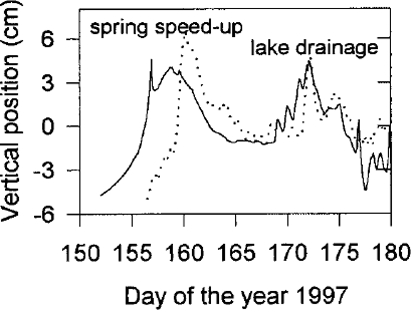
These results show that the uplift events associated with lake drainages could potentially be explained by the expansion of a till layer, mostly of its uppermost part, because the water-pressure variations do not diffuse far into the till. However, comparable model uplift (as in Fig. 11) requires a till compressibility of around 10⁻⁶ Pa⁻¹, which is very high considering the granular nature of recovered till (Reference Truffer, Motyka, Harrison, Echelmeyer, Fisk and TulaczykTruffer and others, 1999). We also assume that a large proportion of the strain is recoverable. Values at the lower end of the plausible range of recoverable compressibility would render till expansion negligible.

The spring speed-up and uplift event could not be matched with the till expansion model. This is probably an indication of its different nature: while lake-drainage events occur a short distance upstream from the study site, the spring speed-up is triggered down-glacier and propagates up-glacier.

We have already discussed the possible abrupt reduction in local overburden pressure in reference to the seismic results of Reference Nolan and EchelmeyerNolan and Echelmeyer (1999a, b).This would also result in a reduction of effective pressure and therefore till expansion. For a 5 m thick till layer, as found at Center, and a more reasonable recoverable compressibility of α _v = 10⁻⁸ Pa⁻¹, a temporary reduction in local overburden of 2 MPa would result in 10 cm of instantaneous till expansion, enough to account for the observed uplift (Fig. 11).

Till in an over-consolidated state can dilate as a result of shearing (Reference Boulton and HindmarshBoulton and Hindmarsh, 1987; Reference Iverson, Hooyer and BakerIverson and others, 1998). Shearing can then produce an increase in porosity until a critical state is reached (Reference ClarkeClarke, 1987). In Reference Truffer, Harrison and EchelmeyerTruffer and others (2000) we propose that shearing happens at considerable depth in the till layer and occurs continuously in time; this till should therefore be in a critical state at any time, and no further dilation would occur as a result of stress changes. It is possible that the shear layer is continuously changing position due to dilatant hardening (Reference Iverson, Hooyer and BakerIverson and others, 1998), causing dilation in that limited portion of the till that was not already deforming. However, the pore water moving into this till would originate from the adjoining till that is itself in the process of consolidating. Therefore, it is unlikely that an overall till expansion can result from dilatancy when the till layer is already actively deforming.

Uplift events could also be caused by vertical strain, but the question is difficult to settle because the magnitude and sign of the vertical strain rates can change with depth (Reference Balise and RaymondBalise and Raymond, 1985; Reference Gudmundsson, Iken and FunkGudmundsson and others, 1997). However, longitudinal surface strain rates measured on Black Rapids Glacier were an order of magnitude too small to account for the observed vertical motion. This, together with detailed measurements on other glaciers (Reference Iken, Fabri and FunkIken and others, 1996), leads us to conclude that vertical straining of the ice is unlikely to explain the entire vertical motion events.

The above discussion indicates that many mechanisms can contribute to vertical motion events on glaciers underlain by massive till layers. Perhaps the most likely mechanism is till expansion as a result of a temporary reduction in overburden pressure and therefore effective pressure (Reference Nolan and EchelmeyerNolan and Echelmeyer, 1999a). Such an event also results in temporary water storage within the till layer. This is discussed in the next section.

Dye tracing

In spring 1993, dye was introduced into a lake draining into Black Rapids Glacier during a motion event. Reference CochranCochran (1995) found an initial peak in dye return, but only a small fraction of the total dye was output during that event. Several other peaks in dye concentration followed in the next 3 weeks, always after another speed-up/lake-drainage event had occurred from different marginal or supraglacial lakes.

The model of till expansion and contraction presented above offers the following explanation for this observation. As water pressures rise, till is expanding and storing water, and with it some dye. When the till contracts again, water and some dye are released into the subglacial hydraulic system. This mechanism of water storage in the till could probably be substantiated with detailed measurements in the proglacial stream, such as electric conductivity or chemical analysis that would show extensive contact with till.

Transfer of basal shear stress

We have put forward a model of glacier–till interaction based on a simple Coulomb-plastic failure criterion that is consistent with our in situ till-deformation measurements. This model allows us to explain velocity variations on different time-scales by increasing bed-parallel shear stresses at the glacier margin, causing larger deformation rates in the ice. The stresses at the margins increase because till beneath the central part of the glacier channel is at or near failure. There are at least three mechanisms linking this till failure and marginal shear stresses: (A) an increase in driving stress, which cannot be supported by till already at failure; (B) an increase in water pressure, which causes an increase in the areal extent of till at failure; and (C) short-term changes in local overburden pressure, which lead to failure of nearby till. These linkages are illustrated in Figure 12.

Fig. 12.

Diagram of the stress transfer mechanisms as explained in the text. A positive correlation is indicated by plus signs, a negative correlation by minus signs (e.g an increase in water pressure leads to a decrease in till strength at the channel center). (A), (B) and (C) correspond to the three mechanisms described in the text.

A characteristic property of a perfectly plastic material is that it cannot accommodate any stress above its failure strength. If a perfectly plastic till is at failure under parts of the glacier and the driving stress is increased, the additional stress must be accommodated at other parts of the bed, such as the glacier margins. Another possibility is stress transfer to so-called sticky spots on the bed (Reference Fischer, Clarke and BlatterFischer and others, 1999). (The location of these stress concentrations could be found by measuring ice deformation close to the bed.) In any case, we propose that velocity changes on decadal time-scales are caused by secular variations in driving stress that cannot be supported by basal till that is already at failure. Any increase in driving stress must then be supported by drag elsewhere, with a consequent increase in ice-deformation rates (A in Fig. 12). In an extreme case, the marginal stresses are large enough to exceed the strength of the ice, and the glacier would shear off its margin, as often occurs during a surge.

We propose a related mechanism for seasonal velocity variations. In Reference Truffer, Harrison and EchelmeyerTruffer and others (2000) we showed that till deformation occurs several meters below the ice/till interface. If the water-pressure distribution in the till is governed by diffusion, then a few meters below the top of the till the pressure will be dominated by an annual cycle which has its minimum delayed until early winter. This causes a delayed cyclical variation in till strength. As the water pressure rises (B in Fig. 12), the till fails. Some of the resistance is then transferred from the locations of the weakened till to the margins, which leads to higher marginal deformation rates and therefore a higher center-line velocity. Modeling results of this stress redistribution are shown in Figure 13, along with the resulting velocity field, for the case when the piezometric depth is raised from 70 to 55 m. Shear stress drops in the center and rises at the flanks of the channel. The higher stresses are amplified by the non-linear ice rheology, leading to a substantial increase in surface speed.

Fig. 13.

Shear stress redistribution. The top panels show shear stress (a) and velocity (b) contours for a depth to the piezometric surface of 70 m. The bottom panels show the same contours for a depth to the piezometric depth of 55 m (c, d).The bold line indicates the area of till at failure. The axes are in kilometers, velocities are in m a⁻¹ and stresses in 100 kPa.

Velocities also vary on time-scales of hours or days. We know from a seismic study (Reference Nolan and EchelmeyerNolan and Echelmeyer, 1999a, b) that the till layer undergoes rapid changes in seismic properties. Following these authors, we suggest that the glacier is locally lifted up as parts of the drainage system are over-pressurized, with a reduction in the overburden pressure in adjacent areas through viscoelastic bridging effects (C in Fig. 12). This brings more till to failure. Again, stress is transferred to the sides, and velocity increases.

Ice-flow models often divide the total motion into de-formational and basal components, that is u _total = u _def + u _basal. These components are then treated independently. Our analysis shows that these two components are linked. Changing basal stress conditions (both and τ _s) can produce greater basal motion at the center of the channel and, at the same time, higher deformational velocities at the flanks. This situation is analogous to that encountered on the Siple Coast ice streams in West Antarctica. There, a weak basal till layer causes a transfer of much of the resistive drag to the margins, leading to concentrated zones with high deformation rates (Reference Echelmeyer, Harrison, Larsen and MitchellEchelmeyer and others, 1994).

Consequences for glacier models and ice-deformation studies

Models of glacier changes, such as those due to changes in mass balance, are determined by the glacier geometry, the rheology of ice and the boundary conditions at the bed and surface. The boundary condition that relates basal velocity to the basal shear stress has perhaps the largest uncertainty. This boundary condition often has the form (Reference WeertmanWeertman, 1957) or that proposed by Reference Budd, Keage and BlundyBudd and others (1979) which accounts for the effective pressure at the bed,

C, m and d are adjustable parameters. However, Reference Iken and TrufferIken and Truffer (1997) have shown that the latter sliding law does not hold, even if the effective pressure distribution is known.

Here, instead, we assume that the model glacier is underlain by a till layer that has a perfectly plastic rheology, which is consistent with our observations beneath Black Rapids Glacier (Reference Truffer, Harrison and EchelmeyerTruffer and others, 2000). We also make the simplifying assumptions that the angle of internal friction is a constant, the pore-water distribution is not affected by till deformation, the piezometric surface is constant across the glacier, and no basal motion occurs where the basal shear stress is below the failure strength of the till. We note that, in particular, the latter two assumptions may not hold in all cases, and the following should therefore be considered as a first approximation only.

For such a model we have calculated “effective shape factors” for flow in parabolic cross-sections of various aspect ratios, W, and various piezometric depths. Table 2 lists the normalized center-line velocity at the surface and the ice flux, where the velocity is normalized by , which is the surface speed of a plane of thickness h (center-line depth) and slope a, and the flux is normalized by . The angle of internal friction is the single parameter describing the material properties of the till (by Equation (1)); we use φ = 30°.

Table 2.

Effective shape factors for parabolic glacier cross-sections

For glaciers underlain by till, Table 2 provides a simple means to calculate ice flux and center-line velocity given an estimate of water pressure. There is an increasing ice flux with higher water pressures because of the increase in the areal extent of till at failure and increased ice deformation at the margins. This increase is particularly pronounced in wide channels, where a larger part of the glacier bed, and thus of the basal till, is affected.

Examination of our model calculations shows that, in most realistic cases of flow in parabolic channels, the shear stress is not generally linear with depth, even on the channel center line. Therefore we caution against the use of a stress shape factor and a linear depth dependence when calculating the shear stress within a glacier. For small values of W (deep, narrow channels) this non-linear stress distribution is present even with no variations in sliding or till deformation across the bed (Reference EchelmeyerEchelmeyer, 1983). In situations of non-uniform basal motion, as presented in this paper, the shear stress deviates considerably from a linear function with depth, as shown in Figure 14. This non-linear shear stress variation complicates the interpretation of borehole deformation data in terms of a flow law relating deformation rate to the components of the stress tensor because it couples basal motion to ice deformation.

Fig. 14.

Center-line shear stress distribution with height above the bed (normalized by the center-line depth of 600 m) for a parabolic channel for different piezometric depths, H. The curves increasingly deviate from a linear stress-depth relation as H is decreased. The model represents a best parabolic fit to Figure 3b.

Till vs bedrock

Observations of fluctuations in surface speed and elevation similar to the ones discussed in this paper have been made on many other glaciers (e.g. Reference WillisWillis, 1995). While we have focused on the explanation of these phenomena in terms of changes within the till layer found beneath one section of Black Rapids Glacier, it is also possible to explain some of them in terms of a model in which clean glacier ice overlies bedrock. Such explanations have been developed in the past, and we summarize a few of them here.

Secular velocity variations have been explained by longterm changes in the subglacial drainage system, such as the interconnectedness of cavities (Reference Iken and TrufferIken and Truffer, 1997). Such changes could occur as a reaction to changes in the glacier geometry. Reference KambKamb (1987) has shown that the stability of a distributed vs an arborescent drainage system depends, among other things, on the basal shear stress. Geometry changes could therefore trigger a switch in drainage systems and with it variations in basal velocity, such as in the surge initiation on Variegated Glacier. It should be noted, however, that borehole drilling through that glacier encountered basal debris and not clean bedrock (Reference Harrison, Kamb and EngelhardtHarrison and others, 1986), so till deformation may have actually played a key role in that surge.

Reference HodgeHodge (1974) related water storage to seasonal velocity changes. Reference Kamb, Engelhardt, Fahnestock, Humphrey, Meier and StoneKamb and others (1994) also found that water storage was a good control variable for basal motion on shorter time-scales, such as the speed-up events on Columbia Glacier. These have been explained in terms of bed separation and cavity formation at a clean glacier bed (Reference LliboutryLliboutry, 1968), as have vertical motion events (Reference Iken, Röthlisberger, Flotron and HaeberliIken and others, 1983, Reference Iken, Fabri and Funk1996).

Thus, similar observations find explanations in an ice–bedrock as well as an ice–till model. We have not succeeded in identifying a characteristic signature of a basal till layer in surface measurements. As far as the velocity distribution in a transverse section is concerned, this can already be recognized by comparing our results with the modeling of Reference ReynaudReynaud (1973) and Reference HarborHarbor (1992), who used a friction law and a sliding law, respectively. They obtained results that were somewhat similar to ours. One therefore needs to exercise care when making inferences about the ice substrate from glacier surface dynamics.