1. Introduction
Mortality forecasting is a crucial topic for actuarial practice, government policy making and demographic research. In order to model liability cash flows, we need to project mortality over the long term. There has been extensive research in this area for developed countries. Booth & Tickle (Reference Booth and Tickle2008) classify mortality modelling and forecasting as three approaches: expectation, explanation and extrapolation. Expectation approach has been employed in the form of expert opinions, which is preferred by many official statistical agencies. Explanation approach relies on structural or causal epidemiological models, which takes causes of death into consideration. Extrapolation approach uses time series techniques and is the basis of most stochastic mortality modelling methods. Lee & Carter (Reference Lee and Carter1992) first build a two-factor stochastic mortality model, which is estimated using singular value decomposition (SVD). Since 2000, many other models have been suggested as alternatives to the Lee–Carter model by adding additional age–period effects such as Hyndman & Ullah (Reference Hyndman and Ullah2007) and Booth et al. (Reference Booth, Maindonald and Smith2002) (see Cairns, Reference Cairns2013). In addition, Currie et al. (Reference Currie, Durban and Eilers2004) use two-dimensional (2D) P-splines for mortality modelling, which is significantly different from the Lee–Carter model. Some other researchers proposed new models by incorporating the year-of-birth effect, such as Renshaw & Haberman (Reference Renshaw and Haberman2006), Cairns et al. (Reference Cairns, Blake, Dowd, Coughlan, Epstein, Ong and Balevich2009) and Richards et al. (Reference Richards, Kirkby and Currie2006). In recent years, coherent stochastic mortality modelling with multiple populations has begun to emerge (see Li & Lee, Reference Li and Lee2005; Cairns et al., Reference Cairns, Blake, Dowd, Coughlan and Khalaf-Allah2011; Li & Hardy, Reference Li and Hardy2011). China is the world’s largest country by population, thus its mortality has significant impact on global mortality. However, only a little research has concentrated on Chinese mortality, principally due to data limitations. Publicly available Chinese mortality data mainly come from three sources: (1) 1% or 0.1% survey data; (2) the population census data; (3) China Death Cause Survey data. Most research uses 1% or 0.1% survey mortality data collected from China Population Statistics Yearbooks (1988–2006) and China Population and Employment Statistics Yearbooks (2007–2012)Footnote 1 and the population census data (1981, 1989/1990, 2000 and 2010)Footnote 2 for mortality modelling and forecasting purposes (e.g. see Wang & Huang, Reference Wang and Huang2011; Zhao, Reference Zhao2012; Zhao et al., Reference Zhao, Liang, Zhao and Hou2013). Some research also uses Chinese mortality data from the China Death Cause SurveyFootnote 3 (see Li & Lee, Reference Li and Lee2005).
All of the existing research uses extrapolative methods to project future Chinese mortality. For example, Li et al. (Reference Li, Lee and Tuljapurkar2004) extend the Lee–Carter method from single-year intervals to unequal intervals to deal with limited data. An application to China is conducted with three observations (1974, 1981 and 1989/1990). Zhao (Reference Zhao2012) introduces a modified Lee–Carter model to analyse short-base-period mortality data, which approximates the unknown parameters by linearised cubic splines and other additive functions to overcome the severely fluctuating predicted age-specific mortality. An application to China demonstrates the advantages of the modified method over existing methods using mortality data from 2000 to 2008. The Chinese mortality rates are then projected to 2010 for both males and females. Employing the same method, Zhao et al. (Reference Zhao, Liang, Zhao and Hou2013) investigate the group-specific (the country (national), cities, towns and counties) mortality in China and find that in general the age-specific mortality rates decrease over the years and the speed of the decrease increased in the past decade. There are also some papers in Chinese using the original Lee–Carter method or its variants to project Chinese mortality (see Lu & Yin, Reference Lu and Yin2005; Wang & Huang, Reference Wang and Huang2011). Although the past decades have seen extrapolative methods successfully applied in some developed countries, these methods require the length of data to be appropriate for projections and reliable results. As discovered by Lee & Carter (Reference Lee and Carter1992), the fitted models and projected mortality values become unstable when the extent of historical data is as short as 10–20 years, which is indeed the case for many developing countries including China. In addition, all pure extrapolative approaches assume that the future trend will follow the historical trend. This is a problem especially for countries with limited data. It is hardly reasonable to assume that the future 50 years will follow the trend in the past 10–20 years for a developing country, as developing countries usually experience fast transformations within decades as in China (see Zhao & Guo, Reference Zhao and Guo2007). To tackle these problems, we propose to model and project Chinese mortality in a way different from a pure extrapolative approach, that is, to use a modified Continuous Mortality Investigation (CMI) Mortality Projections Model developed by the Continuous Mortality Investigation Bureau of the Institute and Faculty of Actuaries (see Continuous Mortality Investigation Committee (CMI), 2009). This approach projects the rates of mortality improvement using a P-spline smoothing method to derive the initial rates of mortality improvement and an expectation method to derive the long-term rates of mortality improvement. A convergence structure from the “initial” to the “long-term” rates of mortality improvement is adopted as the process of projection. The initial rates of mortality improvement are derived using 2D P-spline methodology. Given the short history of Chinese data, the long-term rates of mortality improvement are determined by borrowing information from international experience. We suggest using K-means clustering with dynamic time warping (DTW) distance to classify populations, which is novel in the actuarial mortality research field. One major limitation of the CMI Mortality Projections Model is that it is deterministic. However, in this paper, we make it stochastic using techniques outlined by Koller (Reference Koller2011) and described by Browne et al. (Reference Browne, Duchassaing and Suter2009). Comparing this method with a pure extrapolative approach, we find that the CMI approach is more flexible and suitable for long-term mortality forecasting in China.
The structure of this paper is as follows. Section 2 introduces the data used in this research. Section 3 describes the methodology and presents the modelling results. Section 4 discusses the sensitivity analysis. Section 5 illustrates how to add uncertainties and confidence intervals to the deterministic estimates. Section 6 compares the model applied in this paper with a pure extrapolative approach. Finally, section 7 concludes the paper.
2. Data Sources
From the data sources described in section 1, we could obtain age–sex-specific mortality data from China Population Statistics Yearbooks (1995–2006) and China Population and Employment Statistics Yearbooks (2007–2012) for successive calendar years 1994–2011. However, only 1997–2011 data are available for ages up to 90+. Hence, in this paper we apply age–sex-specific Chinese mortality data from 1997 to 2011 (a total of 15 years) for modelling purposes using a modified CMI Mortality Projections Model. The data retained for the model are for people aged 20–90+ and they consist of central exposures, death counts and central death rates for each age, gender and calendar year. Table 1 summarises the data sources: the data for 2000 and 2010 are from successive censuses; the data for 2005 are from national surveys of 1% of the population; and the data for the other years are from national surveys of around 0.1% of the population.
Data sources.

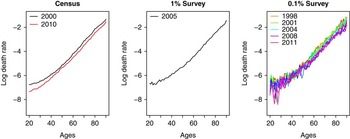
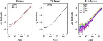
We plot the census data, 1% survey data and 0.1% survey data for males and females in Figures 1 and 2, respectively. It shows that the volatility of 0.1% survey data is significantly larger than that of the census data and 1% survey data, especially at younger ages. This is likely due to the fact that the smaller survey data contain much more noise than the larger survey and census data, especially when the death counts are very small (such as for younger ages).
Plots of log death rates for males: census, 1% survey and 0.1% survey.

Plots of log death rates for females: census, 1% survey and 0.1% survey.

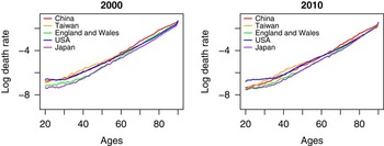
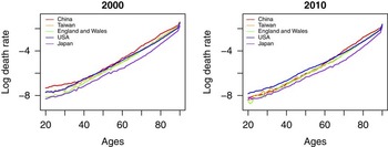
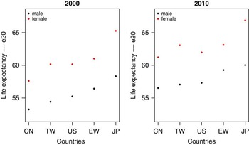
In order to locate Chinese mortality in an international context, we plot the log death rates of China, Taiwan, England and Wales, the United States and Japan for years 2000 and 2010 (the census years in China) for comparison purposes. The plots for males and females are in Figures 3 and 4, respectively. Comparing the mortality of China with that of other countries, we find that both males and females in China have the highest mortality rates for ages older than around 60 in both 2000 and 2010. And for younger ages, the mortality level of China is similar with that of Taiwan and the United States in 2000 and becomes closer to that of England and Wales and Japan in 2010. The improvement of female mortality rates is more significant than males in China. The results indicate that Chinese mortality has improved significantly in the past decade (2000–2010) and is becoming closer to developed countries with low mortality levels. To further exemplify, we plot the period life expectancy of people aged 20 in Figure 5.
Plots of log death rates for males, 2000 and 2010.

Plots of log death rates for females, 2000 and 2010.

Comparison of period life expectancies for people aged 20 in years 2000 and 2010. CN, China; TW, Taiwan; US, United States; EW, England and Wales; JP, Japan.

3. Models and Results
In this section, we use the CMI Mortality Projections Model to forecast Chinese mortality for 40 years, which is an appropriate period for annuity pricing and reserving, as well as long-term planning of social security pensions. There are four inputs to project mortality based on the CMI approach (see CMI, 2009):
-
∙ Base mortality rates q x,t Footnote 4 , where x is age and t the base year.
-
∙ Initial rates of mortality improvement. We denote the rates of mortality improvement as
 $$MI_{{x,t}} {\equals}1{\minus}\left( {q_{{x,t}} \,/\,q_{{x,(t{\minus}1)}} } \right)$$
-
∙ Long-term rates of mortality improvement.
-
∙ Convergence from the initial rate to the long-term rate of mortality improvement.
We discuss each of the inputs and the projection results in this section. The method is employed for males and females, respectively. For the third input – long-term rates of mortality improvement – we will apply a novel technique in the actuarial mortality research field to determine them using clustering techniques. Where not stated, we have followed the CMI exactly.
3.1. Base mortality rates
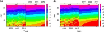
The base mortality rates reflect the estimated current or recent past position. In order to obtain the smoothed base mortality rates, we smooth the mortality surface using age–period P-splines with 4-year knot spacing (see Currie et al., Reference Currie, Durban and Eilers2004). The crude (actual) and smoothed (fitted) log mortality rates are plotted in Figure 6 for males and femalesFootnote 5 . From these plots, we find that the mortality improvement for young ages is bigger than that for older ages. These phenomena are further observed in section 3.2, when discussing the rates of mortality improvement. To the best of our knowledge, these findings are novel in the literature. As for further discussion of the causes of these findings, we leave it for future research.
Plots of the actual/crude (left-hand side of each panel) and fitted/smoothed (right-hand side of each panel) log mortality rates for (a) males and (b) females.

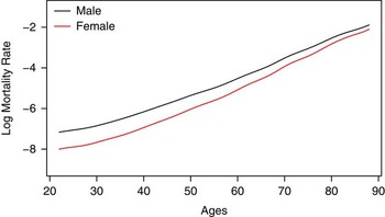
Employing P-spline methodology may introduce unwanted “edge effects”. For example, the final year mortality rates and the initial rates of mortality improvement would be impacted by the final year mortality level of experience. Consequently, future projected mortality would also be influenced year by year. To avoid the “edge effect” which smoothing techniques may be subject to (see CMI, 2009), we choose the base year to be 2 years earlier than the last historical year, that is, 2009; and we remove the top and bottom two ages post smoothing to get the new age range – 22–88. The smoothed log mortality rates for year 2009 are plotted in Figure 7.
Plot of the log base mortality rates, 2009.

3.2. Initial rates of mortality improvement
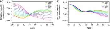
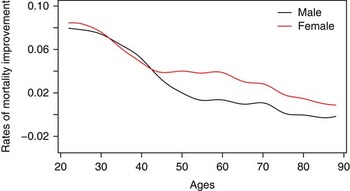
Using the 2D P-spline smoothed mortality rates obtained in section 3.1, we further derive the smoothed rates of mortality improvement, which are shown in Figure 8. The order of the lines (from 1998 to 2011) is the order of the rainbow colours (from red to purple), and applies to all rainbow graphs in this paper. From these plots, we observe that there is not much change in mortality improvement for ages around 50 for both males and females. The range of change for males is larger than that for females. For males, the rates of mortality improvement keep increasing from 1998 to 2011 for ages younger than 50, while for ages older than 50, the rates of mortality improvement are decreasing after several years of increasing. For females, the rates of mortality improvement remain at a higher level for ages 20–30 and then decrease to age 50, while for ages older than 50, the patterns are similar to those for males. It is also interesting to notice that the rates of mortality improvement for males are negative for some ages at some specific years (e.g. the older ages in recent years), while they are all positive for females. That means the mortality rates of males at some ages actually increased at certain times, while the mortality rates of females at all ages consistently decreased over the years.
Rainbow plots of the historical smoothed rates of mortality improvement for (a) males and (b) females, 1998–2011.

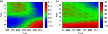
Heatmaps of the smoothed mortality improvement rates are plotted in Figure 9 using the same scale. The black lines indicate different birth cohorts. The original CMI Mortality Projections Model considers the UK data, where the cohort effects are very compelling. In order to capture the cohort patterns, the model decomposes the rates of mortality improvement MI (x, t) for age x in year t by age, period and cohort for each gender using an additive age–period–cohort (APC) model (see CMI, 2009). However in Figure 9, we do not find convincing evidence of a cohort effect in the Chinese female data, and little evidence in the Chinese male data. For example, the 1958 year-of-birth “cohort effect” (for those aged 40 in 1998) is observed as a diagonal feature for males in Figure 9(a), which could be due to the “Three years of natural disasters” (1958–1961) (see Song, Reference Song2009). However, there has not been any detailed investigation into cohort mortality patterns due to the data limitation and we call for future research in this area. As the data covers a short period, it would have little power to separate age/period and cohort effects. The selected initial rates of mortality improvement are plotted in Figure 10.
Heatmaps of the historical smoothed mortality improvement rates for (a) males and (b) females, 1998–2011.

The initial rates of mortality improvement, 2009.

3.3. Long-term rates of mortality improvement
The user is required to set the long-term rates of mortality improvement in the CMI Mortality Projections Model, and this is the single most important parameter for users to set for projections according to the CMI (2009).
The original CMI Mortality Projections Model suggests using an international average rate of mortality improvement over a long historical period. However, in this research, we propose a novel method in the actuarial mortality research field, which introduces classifying worldwide mortality data. This new method could provide more appropriate long-term rates of mortality improvements, as we explicitly identify a group of populations with similarity in mortality rather than potentially arbitrarily choosing a number of populations. This clustering method could be useful not only for setting long-term rates of mortality improvement in the CMI Mortality Projections Model, but also for determining the groups of data for coherent mortality modelling. In the literature on coherent mortality modelling, the majority of papers choose the group of similar populations subjectively (e.g. Li & Lee, Reference Li and Lee2005). Our method could provide researchers more evidence and rationale in choosing appropriate data for modelling purposes.
It would be ideal if we could use all countries in the world for clustering analysis. However this is impossible as mortality data are not available for many countries, especially developing ones. So in this paper, we choose the six European countries with the longest period of data (Denmark, France, Norway, Sweden, England and Wales, and the Netherlands), the United States, Japan, Taiwan and China for discussionFootnote 6 . These countries represent different regions in the world and could be potentially used to determine the long-term rates of mortality improvement for China. All the data (except for China) are obtained from the Human Mortality Database (n.d.)Footnote 7 .
The methodology to determine long-term rates of mortality improvement involves three steps: Lee–Carter decomposition, DTW distance computation and K-means clustering. We introduce each step as follows.
3.3.1. Lee–Carter decomposition
We first fit all populations using the Lee–Carter method (see Lee & Carter, Reference Lee and Carter1992) to decompose the mortality into age and period components. We choose the Lee–Carter method as it has been used extensively both in research and in application. If desired, we could also use other methods to decompose the mortality data. The Lee–Carter model is in the following form:
 $${\rm ln}(m(x,t))\,{\equals}\,\alpha (x){\plus}\beta (x)\kappa (t){\plus}{\it \epsilon}(x,t)$$
where m(x, t) is the central death rate for age x and year t; α(x) and β(x) the age-specific constants; κ(t) the time-varying index; and  (x, t) the error term. This model can be fitted using the SVD method to obtain a least squares solution. The time-varying indexes κ(t) for all populations are used for clustering analysis, as they represent the levels of mortality change for different countries.
3.3.2. DTW distance
In order to do time series clustering, we use DTW to find the optimal alignment and determine the distance between any two time series (see Keogh & Pazzani, Reference Keogh and Pazzani2001). This technique is implemented in R using package “dtw” (see Giorgino, Reference Giorgino2009). DTW is a popular technique that has long been used in speech recognition community, which however has never been used in the actuarial mortality research field to the best of our knowledge. The advantage of DTW distance is that two time series may vary in time and speed, which will be especially helpful for us to evaluate the similarity between any two historical mortality data.
Following Müller (Reference Müller2007), we assume there are two time series X={x
1, x
2, … , x
I
} and Y={y
1, y
2, … , y
J
}, where
 $I,J\in{\Bbb N}$
. We denote the variable space as
 $${\cal F}$$
, then
 $$x_{i} ,y_{j} \in{\cal F}$$
, for i∈[1 : I] and j∈[1 : J]. A local distance measure d is defined below to compare two different variables
 $$x_{i} ,y_{j} \in{\cal F}$$
 $$d\,\colon\,{\cal F}{\times}{\cal F}\to {\Bbb R}\geq 0$$
Generally speaking, d(x i , y j ) is small (big) if x i and y j are similar (different). Then the task is to find an alignment between X and Y having minimal overall distance.
We first define an (I, J) warping path as follows.
Definition 1. Suppose there is a sequence p={p
1, p
2, … , p
K
}, where p
k
=(i
k
, j
k
)∈[1 : I]×[1 : J], and k∈(1, K). An (I, J) warping path is the sequence p, which assigns the element
 $$x_{{i_{k} }} $$
of X to the element of
 $$y_{{j_{k} }} $$
of Y with the following three conditions hold:
-
1. Boundary condition: p 1=(1, 1) and p K =(I, J).
-
2. Monotonicity condition: i 1≤i 2≤ … ≤ i K and j 1≤j 2≤ … ≤j K .
-
3. Step size condition: p k+1−p k ∈{(1, 0), (0, 1), (1, 1)} for k∈[1 : K−1].
Next, we define the total distance of an (I, J) warping path between X and Y.
Definition 2. The total distance d p (X, Y) of an (I, J) warping path p between X and Y is defined as follows:
 $$d_{p} (X,Y){\equals}\mathop{\sum}\limits_{k{\equals}1}^K {d\left( {x_{{i_{k} }} ,y_{{j_{k} }} } \right)} $$
Finally, we define the DTW distance between X and Y.
Definition 3. The DTW distance DTW(X, Y) is defined as the minimal total distance among all possible warping paths between X and Y:
 $${\rm DTW}(X,\,Y){\,\equals\,}d_{{p^{{\asterisk}} }} (X,\,Y){\,\equals\,}{\rm min}\{ d_{p} (X,\,Y)\;\!\mid\!\;p\,{\rm is}\,{\rm an}\,{\rm (}I{\rm ,}\,J{\rm )}\,{\rm warping}\,{\rm path}\} $$
In this research, we choose the same historical time periods for all populations to compute the DTW distances for clustering analysis. The largest overlapping history of data is used for computation and comparison purposes. For populations without China, we use the mortality data with a shared history of 40 years (1970–2009). For populations with China, we use the mortality data with a shared history of 12 years (1998–2009).
3.3.3. K-means clustering
K-means clustering (see MacQueen, Reference MacQueen1967) is a popular and one of the simplest method for clustering analysis. We use K-means clustering with DTW distance to classify the populations into groups. The clustering algorithm consists of four steps:
-
1. Randomly select K points as initial centroids for clusters.
-
2. Assign each data point to the cluster whose centroid is closest to it.
-
3. Compute the new centroid of each cluster using the data points assigned to it.
-
4. Repeat 2 and 3, until the centroids do not change anymore.
The clustering results are as follows. For populations without China (1970–2009), Taiwan, the United States and Japan are Group 1, while all the European populations are Group 2. For populations with China (1998–2009), China, Taiwan and the United States are Group 1, while the remaining populations belong to Group 2. Both male and female data have the same grouping. We choose to use two clusters for two reasons. First, by using within-group sum of distances to select the optimal number of clusters, we find that two clusters are the best. Second, when we increase the number of clusters to three, six European countries would be split into different clusters. This is not sensible given similar socio-economic and geographic conditions among these countries.
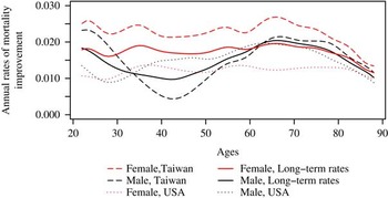
The results are summarised in Table 2. It indicates that in the long term, Taiwan, the United States and Japan have similar mortality patterns; and in the short term, China is more like Taiwan and the United States. We could observe mortality patterns of both Taiwan and the United States in Figures 3 and 4, which indicate that China has more similar mortality patterns with these two countries than with England and Wales. In this case, we set the average rates of mortality improvement of Taiwan and the United States with 40-year history as the baseline of long-term rates of mortality improvement, which are plotted in Figure 11. The average rates of mortality improvement of all the European countries will be used for sensitivity analysis in section 4.1. A useful extension of this work would be to consider applying a coherent method such as the product-ratio method of Hyndman et al. (Reference Hyndman, Booth and Yasmeen2013) to introduce a more explicit judgement on the possible relationship between male and female mortality rates, mortality improvement rates and life expectancies.
Long-term rates of mortality improvement based on Taiwan and the United States.

Clustering analysis on κ(t).

3.4. Convergence from “initial” to “long term”
Following CMI (2009), the convergence process is operated by calculating a weighted average of the initial and long-term rates of mortality improvement. The proportion of the weight placed on the initial rates is determined by fitting cubic polynomials in time.
This mechanism gives full weight to the initial rates of mortality improvement at the start of the projection and to the long-term rates of mortality improvement at the end of the convergence. A parameterised proportion P of the convergence remains halfway through the convergence period. The convergence path is smooth. However, the transition from historical to projected rates may contain an inflection point, as the model does not account for the trend in rates of mortality improvement before the start of the projection (see CMI, 2009: 64).
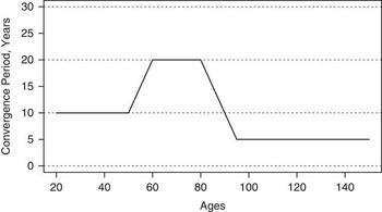
The proportion remaining at the mid-point is determined by users to control the speed of the convergence. Following the core parameter layer in CMI (2009), we set the value of P as 50%. Therefore, the projected rates of improvement at the middle of convergence period will be the average of the initial and long-term rates of mortality improvement. Other values of P will be discussed in the sensitivity analysis in section 4.2. Following the CMI approach, for both males and females we set the period of convergence for the age–period component as follows: 10 years for ages up to 50, increasing by 1 year for each year of age up to 60; 20 years for all ages to 80, and then decreasing by 1 year for each year of age to 88. It implies that the rates of mortality improvement change by decade for younger people (22–50); enjoy a long-running feature due to some major causes of death for older people (60–80); and have a decreasing period of convergence for oldest ages (80–88) to be consistent with the general concept of the rates of mortality improvement running to 0 quickly after age 100 (see CMI, 2009). The period of convergence is illustrated in Figure 12.
Period of convergence.

3.5. Projection results
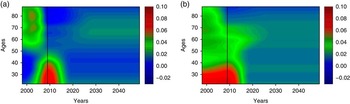
The historical and projected rates of mortality improvement are plotted as heatmaps in Figure 13 for males and females using the same scale. From these plots, we observe that the rates of mortality improvement are projected into the future smoothly. The vertical black lines indicate the year 2009, which is the ending year of the historical period.
Historical and projected mortality improvement rates for (a) males and (b) females, 1998–2049.

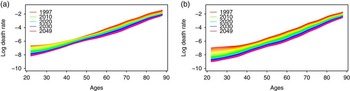
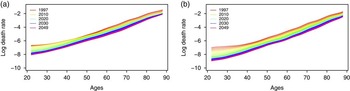
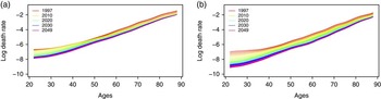
Using the base mortality rates in 2009 and the projected rates of mortality improvement from 2010 to 2049, we obtain the historical and projected mortality rates, which are plotted in Figure 14. We find that the mortality rates smoothly decrease over the years. Furthermore, the mortality level of females improves faster than that of males for younger ages. We note that the gap between Chinese mortality and the mortality of the leading countries (notably Japan) is larger for females than for males, as illustrated in Figures 3 and 4. This may indicate that the mortality of females has more potential to decrease compared with that of males.
Historical and projected log mortality rates for (a) males and (b) females, 1997–2049.

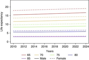
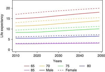
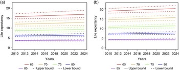
The projected cohort and period life expectancies for males and females with older ages are plotted in Figures 15 and 16. The life expectancies are computed using mortality rates curtate to age 88 to avoid “edge effects”. We observe that there is no crossing among the projected lines. The life expectancies are increasing in the projected period. The speed of improvement in life expectancies for younger people is faster than that for older people. Females will have longer life expectancies than males. We also considered combining the genders to derive long-term mortality improvement rates. However, the relationship between male and female mortality rates over time is a very challenging modelling issue. Research is ongoing in the field of coherent mortality forecasting, specifically sex-coherent mortality forecasting (e.g. the product-ratio method of Hyndman et al. (Reference Hyndman, Booth and Yasmeen2013)).
Projected cohort life expectancy.

Projected period life expectancy.

4. Sensitivity Analysis
We conduct sensitivity analysis for two key parameters in this research, respectively:
-
∙ long-term rates of mortality improvement and
-
∙ the proportion remaining at the mid-point in the convergence process.
4.1. Long-term rates of mortality improvement
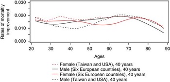
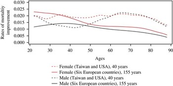
As discussed in section 3.3, we set the long-term rates of mortality improvement using Taiwan and the US mortality data with a history of 40 years. For sensitivity analysis, the long-term rates of mortality improvement are determined by using the six European countries with a history of 40 and 155 years, which are plotted in Figures 17 and 18, respectively. In particular, the longer time period (155 years) gives us an indication of a possible very long-term average rate of change in mortality rates, encompassing periods of higher and lower mortality improvement. Comparing the long-term rates of mortality improvement, we find that the long-term rates of mortality improvement using data from the six European countries with 155-year history are lower than those using data from Taiwan and the United States for all ages of females and for most ages of males (except for ages from 35 to 50). In addition, the long-term rates of mortality improvement using data from the six European countries with 40-year history are similar to the initial long-term rates.
Long-term rates of mortality improvement, Europe, 40 years.

Long-term rates of mortality improvement, Europe, 155 years.

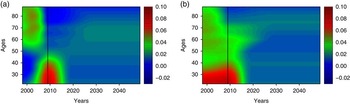
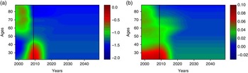
The projected rates of mortality improvement for males and females using the six European countries are shown in Figures 19 and 20. The projection process in Figure 19 is similar to Figure 13 due to the similarity in long-term rates of mortality improvement, while Figure 20 has a relatively different pattern especially for older ages due to the lower rates of mortality improvement. The projected mortality rates are plotted in Figures 21 and 22, which are also smooth and reasonable. The projected cohort life expectancy for males and females are shown in Figures 23 and 24. From these plots, we find that the projected cohort life expectancies in the sensitivity analysis using 155 years of history to compute the long-term rates of mortality are lower than those in the initial (base) model, as there is a clear gap in Figure 18 between the two long-term rates of mortality improvement both for males and females for those ages. However, the projected cohort life expectancies using 40 years of history to compute the long-term rates of mortality are similar to those in the initial (base) model due to the similarity in long-term rates of mortality (see Figure 17).
Projected rates of mortality improvement, sensitivity analysis of long-term rates of mortality improvement (six European countries, 40 years) for (a) males and (b) females, 1998–2049.

Projected rates of mortality improvement, sensitivity analysis of long-term rates of mortality improvement (six European countries, 155 years) for (a) males and (b) females, 1998–2049.

Historical and projected mortality rates, sensitivity analysis of long-term rates of mortality improvement (six European countries, 40 years) for (a) males and (b) females, 1997–2049.

Historical and projected mortality rates, sensitivity analysis of long-term rates of mortality improvement (six European countries, 155 years) for (a) males and (b) females, 1997–2049.

Projected cohort life expectancy for (a) males and (b) females (six European countries, 40 years).

Projected cohort life expectancy for (a) males and (b) females (six European countries, 155 years).

4.2. The proportion remaining at the mid-point
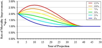
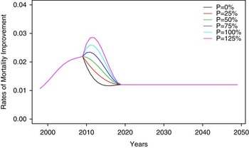
The default proportion remaining at the mid-point for the convergence process is 50%. For sensitivity analysis, we set the proportion remaining at the mid-point as 0%, 25%, 75%, 100% and 125%, which represent speeds of convergence from fast to slow. Figure 25 extracted from CMI (2009) illustrates the operation of the convergence process with various proportions remaining at the mid-point. In order to illustrate the convergence process, we plot the historical and projected rates of mortality improvement with different proportions of convergence remaining at the mid-point for males aged 50 as an example (see Figure 26).
Illustration of the operation of the convergence formula over a 40-year period, with various proportions of convergence remaining at mid-point (CMI, 2009).

Historical and projected rates of mortality improvement for males aged 50.

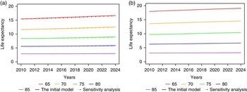
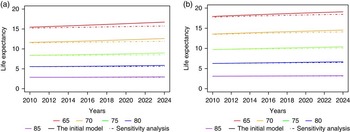
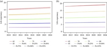
In order to analyse the impacts of various proportions remaining at the mid-point in the convergence process, we use the cohort life expectancy for various ages to show the results, which are presented in Figure 27. We find that for different proportions remaining at the mid-point, the life expectancies for males are slightly different, while for females there is no significant difference. The reason is that for the older ages, the long-term and short-term rates of mortality improvement are very close for females, while there is a gap for males, which can be seen from Figures 10 and 11.
Cohort life expectancy for various ages with various proportions remaining at the mid-point for (a) males and (b) females.

5. Uncertainty Modelling
Using the CMI Mortality Projections Model, we have obtained deterministic estimates for future Chinese mortality. However, nowadays stochastic models are becoming more and more popular and necessary for life insurance portfolios, social security pensions as well as government analysis. By attaching confidence intervals to the best estimate, stochastic models can be much more informative for decision making and improving risk management strategy. However, one major limitation of the CMI Mortality Projections Model is that it is deterministic. So in this section, we add uncertainties to the best estimates obtained from the CMI approach using techniques outlined by Koller (Reference Koller2011) and described by Browne et al. (Reference Browne, Duchassaing and Suter2009).
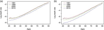
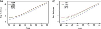
In previous sections we have used data from the censuses, 1% surveys and 0.1% surveys, from 1997 to 2011 for modelling purposes (see Table 1). Although it could provide us with good estimates of the projection of central mortality, this may lead to significantly larger volatility of mortality rates than in reality. The volatility in smaller samples should not influence our estimate of the “true” volatility, which we will use to determine the potential range of outcomes. To prevent that problem, we use data from four censuses to estimate the uncertainty attached to the best estimates. The four census data are for years 1981, 1989, 2000 and 2010. The crude death rates of the four censuses are plotted in Figure 28. We can see that the mortality decline is faster in most recent decade (2000–2010) than in previous decades, which is consistent with the findings in Zhao et al. (Reference Zhao, Liang, Zhao and Hou2013).
Crude log death rates for (a) males and (b) females, 1981–2010.

Suppose q
x
,
t
is the smoothed (expected) mortality and
 $\hat{q}_{{x,t}} $
is the crude (observed) mortality. Using the model described by Browne et al. (Reference Browne, Duchassaing and Suter2009), we have
 $$\hat{q}_{{x,t}} {\,\equals\,}q_{{x,t}} {\times}C_{t} {\plus}{\it \epsilon}_{{x,t}} $$
where C
t
is the stochastic process, which represents the systematic risk; and
x,t
the random noise, which represents the diversifiable risk. We choose to leave the diversifiable risk aside as it can be neglected in the context of large portfolios. To model the systematic risk, we define the stochastic process C
t
as follows:
 $$\eqalignno{ & C_{t} {\,\equals\,}{\rm exp}(X_{t} ){\times}C_{{t{\minus}1}} ,\forall t\,\gt\,0 \cr & C_{0} {\,\equals\,}1 \cr & (X_{i} )_{{i\in N}} \,\sim\,N(\mu ,\sigma ^{2} )\;{\rm i}{\rm .i}{\rm .d} \cr & E[{\rm exp}(X_{t} )]{\,\equals\,}1 \cr & ({\epsilon}_{{x,i}} )_{{i\in N}} \;{\rm i}{\rm .i}{\rm .d},\;E[{\epsilon}_{{x,i}} ]{\,\equals\,}0,\;\forall i \cr & (C_{t} ,{\epsilon})\;{\rm independent} $$
The assumptions of the stochastic process further indicate that
 $$\eqalignno{ & E[C_{t} ]{\,\equals\,}1 \cr & \mu {\plus}0.5\sigma ^{2} {\,\equals\,}0 $$
Hence the simulated mortality will be centred on the chosen best estimate. And there is only one parameter (μ or σ) to be estimated as μ and σ are linked.
To calibrate the model, we use 1D P-splines to smooth the mortality. And the smoothed mortality rates are plotted in Figure 29.
Smoothed log death rates for (a) males and (b) females, 1981–2010.

From equation (6), we derive that
 $$\matrix{ {X_{t} {\,\equals\,}{\rm ln}(C_{t} \,\backslash\,C_{{t{\minus}1}} ),\;{\rm where}\;C_{t} {\,\equals\,}\hat{q}_{{x,t}} \,\backslash\,q_{{x,t}} } \hfill \cr } $$
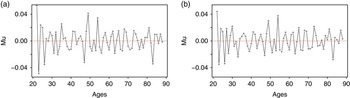
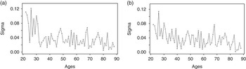
By conducting model validation, we find that C t is independent of age and X t follows a normal distribution. Figure 30 shows the estimated μ for males and females, which fluctuates around 0. Figure 31 shows the estimated σ for males and females. There is a clear break at age 30 for males, which is not that significant for females. Both μ and σ are independent of age, especially for ages from 55 to 85, which is consistent with what has been found in Browne et al. (Reference Browne, Duchassaing and Suter2009). As we only have four time points, the normality assumption of X t is easily accepted using Jarque–Bera tests.
Estimated mu for (a) males and (b) females.

Estimated sigma for (a) males and (b) females.

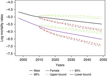
As this methodology is more stable for older ages as discovered by Browne et al. (Reference Browne, Duchassaing and Suter2009) and can be seen in the estimated σ both for males and females (see Figure 31), we suggest to attach uncertainties for ages from 55 to 85. The estimated σ is determined based on all of the past observations for ages from 55 to 85, and the estimated values are 3.10% and 3.19% for males and females, respectively; 95% and 99% confidence intervals for each year are attached to the central estimates in Figure 32 using 1,000 simulations. We could observe a slight turning point for males in the plot, which is from the historical observations. The projected mortality moves smoothly along the historical trend. In addition, the gap between male and female mortality rates is significant and there is no overlapping region for the confidence intervals. The projected cohort life expectancies with 95% confidence intervals for ages 65–85 are shown in Figure 33 using 1,000 simulations. As the 1D P-spline method to smooth the mortality in this section may underestimate the inherent volatility, we could also use a higher value of σ, for example, 4% as suggested by Browne et al. (Reference Browne, Duchassaing and Suter2009), to take that into consideration. The model can now be used for both central estimation and for considering ranges of potential outcomes. For example, in the actuarial context this would include setting appropriate reserves and capital requirements for annuities.
Projected log mortality rates with 95% and 99% confidence intervals for males and females, age=55.

Projected cohort life expectancy with 95% confidence intervals for (a) males and (b) females.

6. Model Comparisons
In this section, we compare the CMI approach with a pure extrapolative approach. In the literature, there are many different extrapolation methods (see Booth & Tickle, Reference Booth and Tickle2008). Using the Bayesian information criterion (BIC) goodness-of-fit model selection criteria, we compare extrapolative models considered in “LifeMetrics”Footnote
8
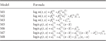
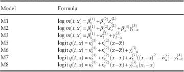
: M1–M8 (except for M4, which is not available), which are analysed in Cairns et al. (Reference Cairns, Blake, Dowd, Coughlan, Epstein, Ong and Balevich2009). Table 3 shows the formulae for the mortality models, where m(t, x) is the death rate, q(t, x) the mortality rate (probability of death),
 $$\beta _{x}^{{(i)}} $$
,
 $$\kappa _{t}^{{(i)}} $$
and
 $$\gamma _{{t{\minus}x}}^{{(i)}} $$
are age, period and cohort components, respectively,
 $\bar{x}$
the average age,
 $\hat{\sigma }^{2} $
the mean value of
 $$(x{\minus}\bar{x})^{2} $$
(see Cairns et al., Reference Cairns, Blake, Dowd, Coughlan, Epstein, Ong and Balevich2009). There are different ways to compute BIC values. In this paper, we use the following definition to be consistent to that used in “LifeMetrics”:
 $$\matrix{ {{\rm BIC}{\,\equals\,}{\minus}{\rm ln}(L){\plus}0.5{\rm ln}(T)\,{\asterisk}\,n} \hfill \cr } $$
where L is the maximised value of the log-likelihood function, n the number of parameters estimated and T the number of observations used for model fitting. So the best model should have the smallest value of BIC. Tables 4 and 5 report the model comparison results for males and females, respectively. We find that the Lee–Carter model (M1) and the Currie APC model (M3) are the best both for males and females in China among all extrapolative models in “LifeMetrics”. In this paper, we show the comparison results of M1 (Lee–Carter model), M3 and M7 models.
Formulae for the mortality models: M1–M8.
Model comparison – male.

Note: BIC, Bayesian information criterion.
Model comparison – female.

Note: BIC, Bayesian information criterion.
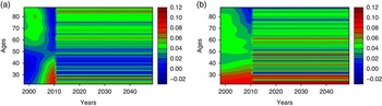
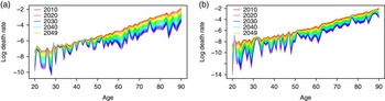
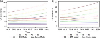
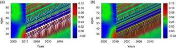
Using the Lee–Carter model, the projected mortality improvement rates for males and females are plotted in Figure 34. We see that the projected rates of mortality improvement are not time dependent, which is not consistent with the historical patterns. In addition, the mortality improvement levels are very high for many ages and are below 0 for some other ages. The projected mortality rates are plotted in Figure 35. The downward pattern by age for many years does not appear realistic. The projected cohort life expectancy for males and females are plotted in Figure 36, which are extremely high both for short-term and long-term projections. So although Lee–Carter model can often be well applied to perform mortality projections for developed countries, it is not appropriate for modelling Chinese mortality given current data quality. These findings are also consistent with the discussion in Lee & Carter (Reference Lee and Carter1992), that the fitted models and projected mortality values become unstable when the extent of historical data is as short as 10–20 years.
Projected rates of mortality improvement for (a) males and (b) females (1998–2049), M1 (Lee–Carter model).

Projected mortality rates for (a) males and (b) females (2010–2049), M1 (Lee–Carter model).

Projected cohort life expectancy for (a) males and (b) females, comparison of Continuous Mortality Investigation (CMI) and M1 (Lee–Carter Model).

We have also tried other extrapolative models and none of them could provide reasonable long-term projections. For example, the projected rates of mortality improvement of M3 and M7 models for males are presented in Figure 37.
Projected rates of mortality improvement (1998–2049), males, (a) M3 and (b) M7 models.

7. Conclusions
In this paper, we use the CMI Mortality Projections Model to project Chinese mortality for long-term actuarial use. The results indicate that the CMI method is an appropriate one in terms of flexibility of use and reasonable outputs. Given the short history of Chinese data, the long-term rates of mortality improvement are determined by borrowing information from international experience. We suggest using K-means clustering with DTW distance to classify populations. By using techniques outlined by Koller (Reference Koller2011) and described by Browne et al. (Reference Browne, Duchassaing and Suter2009), we add uncertainties to the deterministic forecasts for older ages. Comparing this method with a pure extrapolative method, we find that the CMI Mortality Projections Model is more suitable for China to use.
However, this model also has some drawbacks and users should be cautious when using it. For example, although we have added uncertainties for old ages, the uncertainty modelling technique has not been generalised to younger ages. Furthermore, it is challenging to choose a best set of long-term rates of mortality improvement to use and it is difficult to determine the turning point in the convergence process. These uncertain parameters will affect the projected results. Despite these drawbacks, the CMI approach has been applied or suggested in many countries, such as the United States, Canada, United Kingdom and Australia (see The Society of Actuaries, 2013, 2014; Office of the Chief Actuary, 2014; Tang et al., Reference Tang, Browne and Bruhn2014). In the future, it could be employed by more and more practitioners around the world.
For further research, we would like to apply this method to different groups (cities, towns and counties) in China and to explore mortality patterns for these groups (see Paper II). In addition, we would like to develop novel techniques to overcome the drawbacks of this model and make it more reliable and convenient for mortality projections. Finally, we would like to call for collection and distribution of better-quality Chinese mortality data for actuarial modelling and forecasting.
Acknowledgements
The authors would like to thank two anonymous reviewers for their constructive and detailed comments.