








Introduction
The Greenland Ice Sheet is losing mass at an accelerating rate contributing about 10.8 mm to global sea-level rise over the period 1992–2018 (The IMBIE Team, 2023). In addition to increased calving from marine-terminating glaciers, surface meltwater also modulates ice velocity dynamics (Zwally and others, Reference Zwally, Abdalati, Herring, Larson, Saba and Steffen2002; Joughin and others, Reference Joughin, Das, King, Smith, Howat and Moon2008; Bartholomew and others, Reference Bartholomew, Nienow, Mair, Hubbard, King and Sole2010). During the melt season, supraglacial lakes temporarily store large volumes of meltwater that may either overflow gradually through surface channels or abruptly to the bed through hydrofracture (Box and Ski, Reference Box and Ski2007; Selmes and others, Reference Selmes, Murray and James2011; Williamson and others, Reference Williamson, Arnold, Banwell and Willis2017). Once at the bed, this meltwater is routed through a subglacial drainage system that typically evolves from an inefficient distributed network of linked cavities early in the melt season towards a more efficient channelized system of subglacial conduits later in summer, increasing drainage efficiency and altering basal water pressures and ice velocities (Bartholomew and others, Reference Bartholomew, Nienow, Mair, Hubbard, King and Sole2010; Schoof, Reference Schoof2010; Hoffman and others, Reference Hoffman2018). Rapid drainage events serve as a short-term connecting link between the ice surface and bed by altering basal water pressure depending on the capacity of existing subglacial channels (Das and others, Reference Das2008; Tedstone and others, Reference Tedstone, Nienow, Gourmelen and Sole2014). When drainage paths are Inefficient, temporary increases in velocity of up to two- to four-fold have been noticed (Shepherd and others, Reference Shepherd, Hubbard, Nienow, King, McMillan and Joughin2009; Bartholomew and others, Reference Bartholomew2012).
Monitoring supraglacial lakes is critical for quantifying the transfer of meltwater from the ice surface to the bed and understanding its impact on ice dynamics. Over the past decade, a variety of satellite-based studies have advanced our ability to detect and quantify these meltwater systems. Previous studies using MODIS and Landsat satellite imageries have been used to establish the patterns in lake distribution and seasonal evolution but were limited by coarse spatial resolution and cloud cover (Sundal and others, Reference Sundal, Shepherd, Nienow, Hanna, Palmer and Huybrechts2009; Fitzpatrick and others, Reference Fitzpatrick2014). More recently, Sentinel-2’s higher spatial and temporal resolution has allowed lakes to be delineated with markedly improved precision (Williamson and others, Reference Williamson, Banwell, Willis and Arnold2018; Hochreuther and others, Reference Hochreuther, Neckel, Reimann, Humbert and Braun2021). Recent studies using microwave data, EOS-06 Ku-band scatterometer have also revealed anomalous surface melt extent in 2023 over Greenland, demonstrating the value of radar for melt monitoring (Tripathi and others, Reference Tripathi, Mishra, Joshi and Singh2025). Among these studies, the optical thresholding approaches based on normalized difference water indices (NDWI) have achieved lake identification accuracies above 90% when validated against manual outlines. However, misclassification of shadows and slush remains a persistent challenge (Moussavi and others, Reference Moussavi2016; Corr and others, Reference Corr, Leeson, Mcmillan, Zhang and Barnes2022).
For the estimation of lake depth, physically-based radiative transfer equation (RTE) models applied to optical imagery remained the standard approach earlier. Moussavi and others (Reference Moussavi2016) validated RTE-based depths against in-situ sonar measurements, finding red-band methods most suitable with root mean square error (RMSE) values of  $\sim$0.4-0.6 m for lakes shallower than 5 m. Pope and others (Reference Pope2016) achieved RMSE of
 $ \lt 0.38\,\mathrm{m}$ when pairing Landsat 8 green or panchromatic bands with in-situ spectral data. However, optical methods tend to perform poorly for deeper lakes (
 $ \gt $5 m depth) and are highly sensitive to assumptions about lakebed reflectance and water clarity. As mentioned in Melling and others (Reference Melling2024), the green-band RTE models have been shown to overestimate depth by up to 153% while red-band models may underestimate by as much as 63% depending on water properties. Recent advances in satellite altimetry provide a valuable complement to these optical approaches. ICESat-2, which launched in 2018 provides photon-counting lidar measurements at 532 nm wavelength capable of penetrating clear water and detecting subsurface returns. Datta and Wouters (Reference Datta and Wouters2021) developed WATTA algorithm, which processes ICESat-2 ATL03 photon data at an along-track resolution of 0.7 m and has achieved depth estimates with RMSE around 0.39 m when validated against in-situ measurements from Greenland supraglacial lakes. The main limitation of ICESat-2 remains as its 4.1 km along-track beam spacing and 91-day repeat cycle, which provide very high precision along tracks but incomplete spatial coverage across individual lakes as well as the regions of interest. This limitation highlights the advantage of integrated approaches that combine the spatial continuity of optical mapping with the vertical accuracy of altimetry data.
The studies done over Greenland and Antarctica ice sheets have observed instances where rapid drainage of a single supraglacial lake triggers drainage of neighbouring lakes within a few kilometres, a phenomenon termed ‘cascades’ (Banwell and others, Reference Banwell, MacAyeal and Sergienko2013; Christoffersen and others, Reference Christoffersen, Bougamont, Hubbard, Doyle, Grigsby and Pettersson2018). Two major mechanisms may govern these cascade triggering, which are elastic stress transfer from rapid drainage of water, which creates tensile perturbations that destabilize neighbouring lakes (Christoffersen and others, Reference Christoffersen, Bougamont, Hubbard, Doyle, Grigsby and Pettersson2018; Stevens and others, Reference Stevens2024), or the basal hydrological connectivity allows pressurized meltwater to propagate through the subglacial system and promote upward hydrofracture in the adjacent lakes under favourable conditions (Hoffman and others, Reference Hoffman2018; Chudley and others, Reference Chudley, Christoffersen, Doyle, Abellan and Snooke2019). Beyond these two mechanisms, ice flow dynamics may independently modulate rapid lake drainage as in fast-flowing sectors accelerated ice velocities promote tensile fracture propagation and crevasse deepening, which can precondition lake basins to drain rapidly regardless of lake volume or melt intensity (Chudley and others, Reference Chudley2022; Reference Chudley and Howat2025). Recent observations show that about 20% of lakes in Northeast Greenland experienced cascaded drainage between 2017 and 2022 (Lutz and others, Reference Lutz, Tabone, Humbert and Braun2025). In fast-flowing sectors of the ice sheet, interannual velocity variations between melt seasons may therefore contribute to differences in rapid drainage frequency at low elevations, where tensile and compressive stress regimes are most variable (Chudley and others, Reference Chudley and Howat2025). However, the role of topography especially elevation and surface slope in determining where and when cascades start still remains poorly understood. It is also uncertain if the timing and distribution of cascades remain the same across years with different melt intensity. Understanding these changes spatially and temporally is essential for predicting how lake-drainage behaviour might change as extreme melt events become more frequent with ongoing warming.
We focus on the northeast Greenland ice margin, which drains about 12% of the Greenland Ice Sheet with high flow velocities, extensive supraglacial lake coverage and active meltwater-driven subglacial hydrology (Fahnestock and others, Reference Fahnestock, Abdalati, Joughin, Brozena and Gogineni2001; Joughin and others, Reference Joughin, Das, King, Smith, Howat and Moon2008; Hochreuther and others, Reference Hochreuther, Neckel, Reimann, Humbert and Braun2021). Recently observed changes including Zachariæ Isstrøm’s accelerated retreat and 79N Glacier’s surface lowering have heightened the concern about ice stream stability and also making detailed characterization of surface-to-bed meltwater pathways relevant (Mouginot and others, Reference Mouginot2015; Khan and others, Reference Khan2022). Through this study, we combine Sentinel-2 multispectral imagery, ICESat-2 satellite altimetry and Arctic DEM data to map how supraglacial lakes changed in a sub-basin of northeast Greenland during two contrasting melt seasons. The 2019 season had 270.6 positive degree days (PDDs) with consistent warming, marking one of Greenland’s most extreme melt years (Sasgen and others, Reference Sasgen2020; Tedesco and Fettweis, Reference Tedesco and Fettweis2020). In contrast 2020 had moderate cumulative warming of 215.4 PDDs occurring over a shorter and late onset period. This difference in temperature lets us examine how topographic factors influence lake evolution and cascade behaviour under various conditions. We identify rapid drainage events, measure their spatial grouping into cascade sequences and mark the topographic factors that trigger and influence their movement.
Study area and dataset
Study area
This study focuses on the region near two major outlet glaciers draining the Northeast Greenland ice stream, Nioghalvfjerdsfjord Glacier (79 $^\circ$N) and Zachariæ Isstrøm (Fig. 1). The combined basin covers over 650 000 km
 $^2$ making these glaciers significant contributors to Greenland Ice Sheet mass loss and sea-level rise. Both glaciers have undergone rapid changes in recent years. Zachariæ Isstrøm retreated
 $\sim$10 km since 2012 following collapse of its floating ice shelf driven by warm Atlantic water intrusion at the grounding line (Mouginot and others, Reference Mouginot2015). Although 79
 $^\circ$N Glacier has historically remained stable due to its ice tongue buttressing, now it is showing surface lowering and thinning (Khan and others, Reference Khan2022) indicating that it is vulnerable to similar destabilization. Both glaciers develop extensive supraglacial lake coverage during summer melt seasons. This study considers the region near each glacier from approximately 1400 m elevation till the grounding line. This chosen region can capture the range of topographic settings where supraglacial lake formation and drainage occur.
Study area map showing the Nioghalvfjerdsfjord Glacier (79N) and Zachariæ Isstrøm outlet glaciers in the northeast Greenland ice margin (courtesy for background image: ESRI). Elevation contours (brown polylines) derived from the ArcticDEM are shown with a 200 m contour interval and the black circle marks the PROMICE KPC_L automatic weather station location. The red star in the inset map of the Greenland Ice Sheet with basins indicates the study area.

Figure 1 Long description
The map shows the northeast Greenland ice margin highlighting the Nioghalvfjerdsfjord Glacier (79N) and Zachariæ Isstrøm. Elevation contours are marked with brown polylines at 200-meter intervals ranging from 200 to 1400 meters. A black circle indicates the location of the PROMICE KPC_L automatic weather station. The inset map of Greenland shows the study area with a red star. The main map includes longitude and latitude markers with a scale bar indicating 20 kilometers. The glaciers are outlined and the surrounding topography is detailed with contour lines, illustrating the elevation changes across the region.
Datasets
The primary dataset used for mapping the supraglacial lakes was multispectral imagery from the Sentinel-2 mission’s Multi-Spectral Instrument (MSI) (Drusch and others, Reference Drusch2012). Level-2A surface reflectance products were obtained through the Google Earth Engine platform by applying a cloud cover filter of  $\leq$ 20%. The Sentinel-2 products have a 10 m spatial resolution and covers the study area every 3-5 days. This offers detailed tracking of supraglacial lakes during the melt season (Williamson and others, Reference Williamson, Arnold, Banwell and Willis2017; Cooley and others, Reference Cooley, Smith, Ryan, Pitcher and Pavelsky2019).
We used the Ice, Cloud and Land Elevation Satellite-2 (ICESat-2) photon-counting altimetry to develop a depth-reflectance model (Markus and others, Reference Markus2017). ICESat-2’s Advanced Topographic Laser Altimeter System (ATLAS) collects along-track photon-counting measurements at  $\sim$0.7 m spacing with vertical precision better than 0.1 m, making it well suited for supraglacial bathymetry (Markus and others, Reference Markus2017; Neumann and others, Reference Neumann2019; Fricker and others, Reference Fricker2021). The ATL03 geolocated photon heights product was used, which is capable of providing both surface and subsurface returns in clear water conditions. The ability of ATL03 to resolve water-column structure allows accurate depth estimation for calibration of optical reflectance models (Datta and Wouters, Reference Datta and Wouters2021; Lutz and others, Reference Lutz2024; Verma and Vijay, Reference Verma and Vijay2025).
The glacierized area was masked using the Greenland Ice Mapping Project (GIMP) ice mask (Howat and others, Reference Howat, Negrete and Smith2014), which was refined with recent Sentinel-2 imagery. We employed ArcticDEM of 100 m posting (Porter and others, Reference Porter2018) to identify the surface depressions corresponding to potential lake basins which enabled in consistent spatial tracking of lakes through time and topographic characterization of drainage patterns. Daily air temperature data were obtained from the KPC_L automatic weather station of the Programme for Monitoring of the Greenland Ice Sheet (PROMICE) (Fausto and others, Reference Fausto, van As, Ahlstrøm, Colgan, Vandecrux and Box2021; How and others, Reference How2022).
Methods
Supraglacial lake delineation
Supraglacial lakes were detected and mapped using an ensemble approach combining two normalized difference water indices (NDWI $_{\mathrm{ice}}$ and NDWI
 $_{\mathrm{GN}}$ as in Eq. (1) and Eq. (2)) applied to Sentinel-2 multispectral imagery. Pixels were classified as water only when both indices exceeded their specific thresholds. This AND logic strategy reduces the false positive detections from shadows and wet snow while keeping sensitivity to the actual lake features (Doyle and others, Reference Doyle2013; Arthur and others, Reference Arthur, Stokes, Jamieson, Carr and Leeson2020). The methodological flow diagram is represented in Fig. 2
 \begin{equation}
\mathrm{NDWI}_{\mathrm{ice}} = \frac{\mathrm{Blue} - \mathrm{Red}}{\mathrm{Blue} + \mathrm{Red}} = \frac{\mathrm{B2} - \mathrm{B4}}{\mathrm{B2} + \mathrm{B4}}
\end{equation}
 \begin{equation}
\mathrm{NDWI}_{\mathrm{GN}} = \frac{\mathrm{Green} - \mathrm{NIR}}{\mathrm{Green} + \mathrm{NIR}} = \frac{\mathrm{B3} - \mathrm{B8}}{\mathrm{B3} + \mathrm{B8}}
\end{equation}
Flow diagram of the methodology used to extract the supraglacial lake inventory (a) lake mapping and (b) lake depth and volume.

Figure 2 Long description
Three connected sections make up the methodology. Section a, lake mapping, runs two parallel chains. From Sentinel 2 MSI surface reflectance: image selection with cloud cover and shadow masking, computing water indices, tile based Otsu thresholding, raster to vector conversion, basin assignment, post processing, and a lake inventory. From ArcticDEM: fill depressions, identify sinks where filled, and assign unique basin IDs, which feeds the basin assignment step. Section b, lake depth and volume, starts from ICESat 2 ATL03: the WATTA algorithm on ATL03 photons, surface and bottom profile extraction with refractive correction, depth sample extraction from simultaneous ICESat 2 passes, pairing ICESat 2 depth with Sentinel 2 green reflectance, and deriving depth and volume. Both sections feed a bottom data integration box: a unified supraglacial lake database holding area, depth and volume with basin ID.
Spectral water indices based dynamic thresholding
The first index NDWI $_{\mathrm{ice}}$ uses differences in blue–red reflectance, where B2 is the blue band (490 nm) and B4 is the red band (665 nm) (see Eq. (1)). This combination effectively differentiates liquid water from snow, slush and bare ice due to its strong water absorption in red wavelengths and high reflectance in blue (Yang and Smith, Reference Yang and Smith2013; Williamson and others, Reference Williamson, Arnold, Banwell and Willis2017; Arthur and others, Reference Arthur, Stokes, Jamieson, Carr and Leeson2020). However, NDWI
 $_{\mathrm{ice}}$ is sensitive to shaded or wet areas which can mimic water spectra. To address this, the green–NIR index (NDWI
 $_{\mathrm{GN}}$) was incorporated (McFeeters, Reference McFeeters1996), where B3 is the green band (560 nm) and B8 is the near-infrared band (842 nm) (see Eq. (2)). The NDWI
 $_{\mathrm{GN}}$ utilizes strong NIR absorption by water providing complementary discrimination from shadows and wet snow. We applied an AND-voting scheme to classify pixels as water only when both indices met their independent thresholds.
To accommodate spatial variations in illumination, atmospheric effects and surface characteristics while maintaining objectivity, we partitioned the study area into 10  $\times$ 10 km processing tiles and applied Otsu’s method independently to each spectral index within each tile. This dynamic thresholding approach enables threshold adaptation to local surface conditions while preserving reproducibility. Otsu’s method determines an optimal threshold by maximizing the between-class variance that separates water and non-water pixel populations. For each index the method calculates as in Eq. (3), where
 $\omega_0(t)$ and
 $\omega_1(t)$ represent the probabilities of the non-water and water classes separated by threshold
 $t$, and
 $\mu_0(t)$ and
 $\mu_1(t)$ are their respective mean index values (Otsu, Reference Otsu1979). This iterative approach has been successful in detecting supraglacial lakes across multiple glacial environments (Yang and others, Reference Yang2021).
 \begin{equation}
t^* = \arg\max_t \bigl[ \omega_0(t) \omega_1(t) \bigl( \mu_0(t) - \mu_1(t) \bigr)^2 \bigr]
\end{equation}
These derived thresholds were constrained to published ranges to ensure robustness when histogram distributions are anomalous (e.g., extensive cloud cover, shadows or wet snow). NDWI $_{\mathrm{ice}}$ thresholds were set to greater than 0.15 and NDWI
 $_{\mathrm{GN}}$ thresholds to greater than 0.10. These limits have been decided from the previous studies (Moussavi and others, Reference Moussavi2016; Williamson and others, Reference Williamson, Arnold, Banwell and Willis2017; Corr and others, Reference Corr, Leeson, Mcmillan, Zhang and Barnes2022) showing the typical ranges of 0.15 to 0.25 and greater than 0.10 respectively over the glacial regions. Topographic shadows from steep slopes and shadows within the waterbodies can sometimes be misclassified as water due to their low reflectance values. To address this, pixel brightness was calculated by summing the reflectance values of the blue, green and red bands (B2 + B3 + B4). A focal mean filter with a 5-pixel radius was then applied to reduce noise from isolated dark features while retaining larger shadow areas. Pixels with mean brightness below 300 digital numbers were masked as shadows following the threshold established by Williamson and others (Reference Williamson, Arnold, Banwell and Willis2017) for Greenland Ice Sheet conditions using a logical AND operation to retain only water pixels in illuminated areas.
Post-processing
The binary water masks had residual noise from sensor artefacts and slight topographic variations. Connected water pixel groups were filtered by area to eliminate false features, retaining only lakes with an area of 0.0018 km $^2$ or larger (1800 m
 $^2$, equivalent to 18 pixels at 10 m resolution). This threshold was in the published ranges of 0.0009 to 0.0025 km
 $^2$ with a better balance between reducing noise and keeping small yet real supraglacial lakes (Moussavi and others, Reference Moussavi, Pope, Halberstadt, Trusel, Cioffi and Abdalati2020; Hochreuther and others, Reference Hochreuther, Neckel, Reimann, Humbert and Braun2021).
Supraglacial lakes form preferentially in surface depressions controlled by underlying bedrock topography (Selmes and others, Reference Selmes, Murray and James2011; Hochreuther and others, Reference Hochreuther, Neckel, Reimann, Humbert and Braun2021). To enable consistent tracking of individual lakes across the study period, each detected lake was attributed to its corresponding topographic sink. As the multiple lakes can form within the same topographic sink either as separate water bodies or as lakes that subsequently merge or split over time, individual lakes were distinguished using a sequential identifier appended to the topographic sink ID. We identified potential lake basins using the ‘fill_depressions’ tool in WhiteboxTools™ toolbox Lindsay (Reference Lindsay2016), which locates closed topographic depressions by calculating the difference between the original digital elevation model (ArcticDEM, 100 m posting) and a hydrologically-corrected version where all depressions are filled to their pour point elevation. The surface depressions were identified as areas where this elevation difference exceeded 0.5 m, indicating basins with sufficient depth to retain meltwater (Hochreuther and others, Reference Hochreuther, Neckel, Reimann, Humbert and Braun2021). A 3  $\times$ 3 majority filter was applied to the resulting sink mask to reduce noise from minor elevation artefacts. With this, each topographic depression received a unique identifier, forming a stable system for tracking individual lakes across multiple observation dates.
For the temporal analysis of the time series evolution of supraglacial lake systems, we selected an observation-date scheme for representation. All Sentinel-2 Level-2A scenes were manually inspected to identify dates with cloud cover  $\leq 20\%$, cloud shadows
 $ \lt 5\%$ and full spatial coverage across the study area. The manual validation involved in this process is (1) true-colour RGB composite visual inspection to identify cloud contamination and atmospheric haze not captured by automated QA60 masking, and (2) mosaiced imagery verification to ensure adequate coverage across all Sentinel-2 granule boundaries overlapping the study region across different elevation ranges used in this study. All time-series lake statistics (area, depth, volume, drainage events) reported in this study are based exclusively on these dates, termed ‘full-coverage dates’ throughout the paper. In the time-series figures, discrete full-coverage dates are connected using a shape-preserving piecewise cubic Hermite interpolating polynomial (PCHIP), which yields a smooth curve that passes through all observed values while preserving monotonic segments and avoiding spurious oscillations between dates (Fritsch and Carlson, Reference Fritsch and Carlson1980).
Lake depth and volume estimation
Supraglacial lake depths were estimated by combining ICESat-2 ATL03 photon altimetry data with Sentinel-2 multispectral reflectance data by following the framework of Datta and Wouters (Reference Datta and Wouters2021). ICESat-2’s Advanced Topographic Laser Altimeter System (ATLAS) employs photon counting lidar technology operating at 532 nm wavelength, which is capable of penetrating clear water and detect returns from both the water surface and bottom bed under favourable conditions. Despite the satellite’s 91-day repeat cycle and narrow ground track coverage ( $\sim$14 m footprint), the high vertical accuracy (
 $\leq$ 0.1 m) and fine along-track resolution (0.7 m) of individual photon measurements make ICESat-2 an invaluable source of reference depth data for calibrating optical depth retrieval algorithms (Neumann and others, Reference Neumann2019). Lake depth measurements were derived from ICESat-2 ATL03 geolocated photon heights using the WATTA algorithm (Datta and Wouters, Reference Datta and Wouters2021), which processes individual photons at 0.7 m along-track resolution. WATTA uses kernel density estimation to find elevation surfaces, such as the water surface and lake bed and also applies the refractive corrections (
 $n = 1.33$) to convert apparent photon depths to true depths. A quality control procedure was also included to exclude segments with insufficient photons, excessive surface roughness or high turbidity. We selected 10 ICESat-2 passes over lakes during 2019-20, where cloud-free Sentinel-2 imagery was available on the same date. For each pass, green-band reflectances were extracted at every 10 m spatially spaced ICESat-2 photon location. The green band provides superior depth sensitivity compared to the other visible bands, particularly for deeper lakes where blue saturation and red absorption limit optical penetration. This yielded 222 WATTA-derived depths from which outliers exceeding 2.5 times the median absolute deviation were removed to exclude data affected by sensor noise or high sediment load, leaving 189 high-confidence calibration sample depths. These depths have been combined with Sentinel-2 green band reflectance to develop an empirical depth model. Model coefficients were estimated through non-linear least squares regression relation as in Eq. (4) following Box and Ski (Reference Box and Ski2007).
 \begin{equation}
D = \frac{\alpha_0}{R + \alpha_1} + \alpha_2,
\end{equation}
where  $D$ is depth (m) and
 $R$ is the green-band surface reflectance. Using 189 calibration depths, best-fitting coefficients of
 $\alpha_0 = 4.398$,
 $\alpha_1 = 0.310$ and
 $\alpha_2 = -3.710$ were obtained. This model suggests a theoretical maximum retrievable depth of 10.5 m as reflectance approaches zero. Lake volumes were calculated as the summation of pixel area
 $\times$ pixel depth.
Rapid drainage event detection and cascaded cluster identification
Rapid drainage events were identified using two primary criteria: (1) event duration and (2) volume and area loss. A drainage event was classified as rapid if it is completed within 1 to 3 days between successive ‘full-coverage dates’ observations, and resulted in a  $\geq$ 50% reduction in both pre-drainage lake volume and area. This approach helps us differentiate rapid hydrofracture drainage from gradual processes of surface-channel drainage, which usually takes weeks and has less than 30% daily volume loss (Das and others, Reference Das2008; Selmes and others, Reference Selmes, Murray and James2011) or refreezing of lakes. This definition follows earlier observational studies that use abrupt lake lowering over a few days as a proxy for rapid drainage (Box and Ski, Reference Box and Ski2007; Das and others, Reference Das2008; Selmes and others, Reference Selmes, Murray and James2011; Williamson and others, Reference Williamson, Banwell, Willis and Arnold2018) and does not assume a unique physical mechanism. Rapid reductions in area and depth can result from hydrofracture-driven drainage to the bed, enlargement of pre-existing moulins or channels or elastic-stress-triggered cascades initiated by neighbouring lakes (Christoffersen and others, Reference Christoffersen, Bougamont, Hubbard, Doyle, Grigsby and Pettersson2018; Chudley and others, Reference Chudley, Christoffersen, Doyle, Abellan and Snooke2019). For each supraglacial lake, these criteria were evaluated at each consecutive full-coverage observation date by aggregating contributions from all lakes in the same topographic basin. We counted each continuous drainage as a single event by tracking volume and area decreases across consecutive dates to avoid counting intermediate observations as separate events. We recorded variables such as drainage start and end dates, pre and post-drainage volume and area and volume and area loss percentages for each such event.
Potential cascade clusters were identified using a graph-based approach where nodes represent individual drainage events and edges connect events within defined spatial and temporal proximity windows. The spatial proximity was the distance between lake centroids, where we used a 3 km threshold, which approximates the effective radius of elastic stress perturbations capable of triggering downstream hydrofractures up to around 2-5 km distance as mentioned by Christoffersen and others (Reference Christoffersen, Bougamont, Hubbard, Doyle, Grigsby and Pettersson2018). Temporal proximity was drainage initiation dates separated by  $\leq$ 5 days by following observed lag times in cascade studies (Christoffersen and others, Reference Christoffersen, Bougamont, Hubbard, Doyle, Grigsby and Pettersson2018). Each cluster was characterized by its size (number of rapidly drained lakes), maximum pairwise distance between individual lakes (spatial extent) and total drainage duration (time from first to last event). These metrics can be used to test whether cascade behaviour is topographically controlled.
Error assessment and validation
Lake detection and area validation
The automated lake detection algorithm was assessed against 92 manually outlined lakes across four regions of interest in the study area, covering both melt seasons. Manual outlining was done through visual examination of Sentinel-2 true-colour composites. The automated algorithm correctly identified 90 out of 92 lakes, achieving a detection rate of 97.8%  $\pm$ 0.7%. The unmatched lakes (2 out of 92 basins, 2.2%) were mostly very small (
 $ \lt 0.005\,\mathrm{km}^2$), which aligned outside the detection through this methodology. This rate aligns with limitations found in recent studies on supraglacial lake mapping (Williamson and others, Reference Williamson, Banwell, Willis and Arnold2018; Cooley and others, Reference Cooley, Smith, Ryan, Pitcher and Pavelsky2019). The mean absolute area difference calculated between automated and manually delineated lakes was 5.7%
 $\pm$ 3.8%. This indicated a close agreement in the definition of lake boundaries across various lake sizes and surface conditions.
Lake depth validation
The depth model was validated against independent in-situ sonar measurements from Lutz and others (Reference Lutz2024), collected on 8 July 2022 on Zachariæ Isstrøm using a remotely controlled boat equipped with a Lowrance Elite 7 FS sonar sensor ( $\pm$0.11 m precision). Sonar transects extended approximately 100 m into each lake with systematic measurement spacing. We aggregated sonar measurements to 30 m spatially using median statistics and compared these to this study 10 m Sentinel-2-based derived depths. The validation across 58 pixel depths from two lakes (Lake-522, Lake-610b) together yielded RMSE of 0.69 m,
 $R^2$ of 0.82 and MAE of 0.56 m. These metrics were comparable to Lutz and others (Reference Lutz2024), who reported RMSE of
 $\sim$0.80 m and
 $R^2$ of
 $\sim$0.76 for sonar-calibrated and ICESat-2-calibrated depth equations on northeast Greenland lakes.
Depth estimates can also have uncertainty from other sources such as cloud/shadow cover over the water feature and high water turbidity. The ICESat-2-based WATTA algorithm-derived depths contain 0.3-0.8 m uncertainty based on water clarity, photon density and signal-to-noise characteristics as reported in Datta & Wouters (2021). These uncertainties carry over into our Sentinel-2 calibration model. The depth saturation limit of 10.5 m (when reflectance nears zero) could suggest the light loss in clear meltwater (Sneed and Hamilton, Reference Sneed and Hamilton2007; Lutz and others, Reference Lutz2024). Lakes exceeding this depth cannot be resolved with our optical method.
Results
Inter-annual variability of supraglacial lakes
Surface water appearance was used as the indicator for supraglacial lake detection. Supraglacial lakes started to appear in late May for both years with a 4-day difference in onset timing. In 2019, the lake formation initiated on 25 May at a mean surface air temperature of  $-3.8^\circ$C (taken from PROMICE AWS station KPC_L), while in 2020 onset was delayed to 29 May at
 $-2.3^\circ$C as illustrated in Fig. 3. In both years, lakes appeared under subfreezing conditions indicating that meltwater was able to accumulate in surface depressions before the development of sustained positive surface air temperatures. The maximum lake count in 2019 was found on 30 July with 376 lakes covering 234.6 km
 $^2$, whereas in 2020 the maximum count with 385 lakes covering 213.9 km
 $^2$ was detected on 24 July. Although both years observed near similar maximum lake count, the total lake area was nearly 10% lower in 2020.
Time series showing seasonal evolution of supraglacial lakes and surface air temperature for (a) 2019 and (b) 2020. The blue axis (left axis) represents the total daily count of supraglacial lakes, and the orange axis (left axis) shows the total daily lake area (km $^2$). The black axis (right axis) indicates the daily mean surface air temperature (
 $^\circ$C) from the PROMICE KPC_L automatic weather station marked as light blue and red bar plots for positive and negative temperatures, respectively. Points are considered for Sentinel-2 full coverage dates.

Figure 3 Long description
The image contains multiple graphs comparing supraglacial lake counts, lake area and surface air temperature for 2019 and 2020. Each year is divided into four panels based on elevation bands: below 400 meters, 400 to 800 meters, 800 to 1000 meters and above 1000 meters. The x-axis represents dates from May to September, while the y-axis on the left shows the number of lakes and lake area in square kilometers and the y-axis on the right shows temperature in degrees Celsius. For 2019, the maximum lake count occurred on July 30 with 376 lakes covering 234.6 square kilometers. In 2020, the peak was on July 24 with 385 lakes covering 213.9 square kilometers. The graphs show small, medium and large lakes with different line styles and temperature is indicated by shaded regions above and below 0 degrees Celsius. Key trends include the onset of lake formation in late May, peaks in late July and declines towards September. Temperature influences lake formation, with lakes appearing under subfreezing conditions. Differences between years are noted in the timing and extent of lake formation, with 2020 showing a slightly lower total lake area despite a higher count. Visual differentiation includes line styles for lake sizes and shading for temperature thresholds.
The year 2019 was the second-warmest on record over the Greenland Ice Sheet during 2000–20 (Sasgen and others, Reference Sasgen2020; Tedesco and Fettweis, Reference Tedesco and Fettweis2020). During this season, cumulative PDDs reached 270.6, which is about 26% higher than 2020 with 215.4 PDDs. Days having sustained lake presence with more than 200 lakes persisted for 82 days in 2019 (from 14 June to 3 September with 28 observation dates), whereas they stayed for 59 days in 2020 (from 29 June to 26 August with 12 observation dates) marked as persistence in Fig. 3. This difference clearly indicates the shorter melt period in 2020 and the reduced duration of widespread lake presence in the cooler year.
Based on our analysis, supraglacial lakes followed three characteristic patterns of evolution defined by the behaviour of total lake area through the melt season (Fig. S2). An initial build-up from first lake appearance to the seasonal maximum total area is referred to as the growth phase. A mid-season period during which total area remains close to its maximum ( $\geq$ 70% of the seasonal peak and rate of change of area
 $\leq$ 0.2 km
 $^2$/day) is termed the sustained phase and represents a near-equilibrium state in which meltwater input and drainage are approximately balanced, allowing only minor short-term fluctuations. A late-season interval when lake area and numbers decrease rapidly as lakes drain, overflow or refreeze, is referred to as the decline phase.
The growth phase lasted 70 days in 2019 (25 May-2 August) and 57 days in 2020 (29 May-24 July). Total lake area increased at similar average rates (3.95 and 3.75 km $^2$/day, respectively), and lake counts grew at
 $\sim$5-6 lakes/day in both years. Despite this similarity in growth rates, cumulative thermal forcing differed substantially with 203.8 PDDs in 2019 versus 129.2 PDDs in 2020 reflecting the longer duration and sustained warming of the 2019 season. The sustained phase persisted for 19 days in 2019 (2-20 August) and 14 days in 2020 (24 July-6 August). Both total lake area and lake count declined modestly during this period in both years. A notable interannual contrast emerged in volume behaviour. In 2019, the total volume continued to increase slightly despite the gradual reduction in area, suggesting preferential persistence and deepening of larger lake basins. While in 2020, volume declined in parallel with area loss indicating a more uniform drawdown across all lake-size classes. The decline phase lasted 32 days in 2019 (20 August-20 September) and 36 days in 2020 (6 August-10 September). Lake area decreased more rapidly in 2019 (
 $\sim$6 km
 $^2$/day) than in 2020 (
 $\sim$4 km
 $^2$/day), consistent with the steeper late-season temperature drop in 2019 (0.44
 $^\circ$C/day vs. 0.31
 $^\circ$C/day). By contrast, 2020 retained substantially more late-season warming (46.8 PDDs vs. only 9.6 PDDs in 2019), which likely slowed the final drainage and refreezing of the remaining lakes.
Topographic controls on supraglacial lake evolution
To better understand the spatial variability in supraglacial lake formation and persistence, we examined how local topography influences their distribution and characteristics. Two primary topographical parameters such as surface elevation and slope were derived from the 100 m ArcticDEM mosaic. Elevation and slope ranges were defined such that each category contained a comparable number of lake observations. Elevation was divided into four ranges as  $ \lt 400\,\mathrm{m}$, 400-800 m, 800-1000 m and
 $ \gt $1000 m. Similarly, surface slope was classified into three ranges as gentle (
 $ \lt 0.3^\circ$), moderate (0.3-1
 $^\circ$) and steep (
 $ \gt $1
 $^\circ$). The following subsections describe how these topographic factors influenced lake number, area and depth during the 2019 and 2020 melt seasons.
Elevation controls
Supraglacial lake distribution showed systematic elevation-dependent variations in formation timing, number, size and depth (Fig. 4). In 2019, lake formation advanced progressively up-glacier, beginning at  $ \lt 400\,\mathrm{m}$ on 20 May, at 400–800 m on 22 May, 800-1000 m on 23 May and
 $ \gt $1000 m on 24 May with a four-day lag from the lowest to highest elevation ranges. The timing of maximum lake abundance followed a similar trend with lake number peaking below 400 m in mid-June, whereas lakes
 $ \gt $1000 m reached their maximum not until early August. In 2020, this elevation-dependent progression was more compressed with lake onset occurring almost simultaneously across elevation ranges and maximum number reached concentrated within a narrower temporal window.
Time series showing elevation dependence of supraglacial lake formation timing and number in (a) 2019 and (b) 2020. Curves show the daily number of lakes within four elevation regions: below 400 m, 400-800 m, 800-1000 m and above 1000 m with the area category of small, medium and large lakes. The lapse rate corrected mean daily temperature is plotted in the background with red (positive temperature) and blue (negative temperature) bars. Points marked are considered for Sentinel-2 full coverage dates.

Figure 4 Long description
The multi-line graph consists of two panels labeled a and b, showing median lake depth in meters over time from May 15 to September 30. The vertical axis represents median lake depth in meters and the horizontal axis represents the date. Four elevation ranges are depicted: less than 400 meters, 400 to 800 meters, 800 to 1000 meters and greater than 1000 meters. Lines are visually distinguished by different styles. Panel a (2019): - Less than 400 meters: Peaks around mid-June at approximately 3 meters, remains stable and decreases by late September. - 400 to 800 meters: Gradual increase, peaking in mid-July at about 2 meters, then stabilizing. - 800 to 1000 meters: Similar trend to 400 to 800 meters, peaking slightly lower. - Greater than 1000 meters: Peaks in early August, reaching around 2 meters, then declines. Panel b (2020): - Less than 400 meters: Peaks in mid-July at approximately 4 meters, then decreases by late September. - 400 to 800 meters: Peaks in mid-August at about 3 meters, then declines. - 800 to 1000 meters: Peaks in late August, reaching around 2 meters. - Greater than 1000 meters: Peaks in early September, reaching around 2 meters, then drops to near zero by the end of September. Overall, the graph shows elevation-dependent variations in lake depth, with lower elevations generally peaking earlier and higher elevations peaking later. Panel a shows more gradual changes compared to panel b, which exhibits sharper peaks and declines.
The lake size distributions were broadly consistent across different elevation ranges. Small lakes (area  $ \lt $0.5 km
 $^2$) covered more than 80% of the total number in all elevation ranges while medium-sized lakes (area: 0.5-2 km
 $^2$) accounted for about 15 to 18%. Large lakes (
 $ \gt $2 km
 $^2$) were less, representing less than 2% of all mapped features. The lake number also varied systematically with elevation (Fig. 4). The 400-800 m elevation range consistently hosted the largest number of lakes, peaking at 137 in 2019 and 141 in 2020. The 800-1000 m elevation range was the second most active with 112 lakes in 2019 and 115 in 2020. While the
 $ \gt $1000 m elevation range supported the fewest (63 in 2019; 59 in 2020). Overall, the mid-elevation ranges between 400 and 1000 m dominated the lake population accounting for roughly two-thirds (
 $\sim$66%) of all lakes at seasonal peak in both years.
Lake depth decreased systematically with elevation (Fig. 5). The maximum of median depths in the  $ \lt $400 m elevation range reached 4.2 m in 2019 and 3.8 m in 2020, which is
 $\sim$40% greater than those at 800-1000 m, where median depths were 2.5 m and 2.8 m, respectively. The highest elevation range (
 $ \gt $1000 m) contained the shallowest lakes with maximum median depths below 2 m in both years.
Time series of median lake depth by elevation range for (a) 2019 and (b) 2020. Each coloured line represents median depth for a distinct elevation range. Shaded regions indicate interquartile range (IQR). Points marked are considered for full coverage dates.

Figure 5 Long description
The graphs compare the number of lakes over time for 2019 and 2020, split by lake appearance aspect: steep, moderate and gentle. The x-axis represents dates from May 15 to September 30 and the y-axis shows the number of lakes, ranging from 0 to 150. Each panel contains three lines representing different lake sizes: small (area less than 0.5 square kilometers), medium (area 0.5 to 2 square kilometers) and large (area greater than 2 square kilometers). The lines are visually distinguished by different styles. In 2019, for steep aspects, the number of lakes peaks around mid-July, with small lakes showing the highest count. Moderate aspects show a gradual increase, peaking in early August, with medium lakes dominating. Gentle aspects have a steady rise, peaking in late July, with small lakes leading. In 2020, steep aspects show a similar pattern to 2019, with a peak in mid-July. Moderate aspects peak slightly earlier than in 2019, with medium lakes again leading. Gentle aspects show a peak in late July, similar to 2019, with small lakes having the highest count. Annotated durations indicate specific periods, such as ′4-7 days′ and ′4-2 days′, highlighting notable changes in lake numbers. Overall, the graphs illustrate seasonal variations and differences in lake size distribution across different aspects and years.
Slope controls
A systematic slope-dependent variation is seen in the lake evolution (Fig. 6). The gentlest slopes ( $ \lt $0.3
 $^\circ$) contained the most number of lakes (185 in 2019 and 200 in 2020). The moderate slopes (0.3-1
 $^\circ$) supported intermediate counts of 114 (2019) and 105 (2020), while steep slopes (
 $ \gt $1
 $^\circ$) had fewest at 77 (2019) and 80 (2020). Overall, 49-52% of lakes formed on the gentlest terrain while only 20–21% formed on steeper slopes. Despite the higher number of lakes on gentle terrain, these ranges produced shallower water depth (Fig. 7). The maximum median depths on slopes
 $ \lt $0.3
 $^\circ$ reached 1.9 m in 2019 and 3.5 m in 2020, while lakes forming on steeper slopes were considerably deeper with median values of 3.6 m and 4.3 m, respectively. Thus an inverse relationship persisted throughout both melt seasons as flatter surfaces hosted many small and shallow lakes, whereas fewer but deeper lakes formed on steeper terrain where topographic confinement enhanced water retention. Interannual variations in lake depth also differed by slope ranges. The median depth increased from 3.6 to 4.3 m (a 19% rise) on steep slopes while on gentle slopes the deepening was much greater with an 84% increase from 1.9 to 3.5 m. The gentlest slopes stored more total water volume due to their higher lake count despite producing shallower individual lakes in both seasons.
Time series of lake count by slope range for (a) 2019 and (b) 2020. The subplots represent three slope ranges with gentle ( $ \lt $0.3
 $^\circ$), moderate (0.3-1
 $^\circ$) and steep (
 $ \gt $1
 $^\circ$) for three categories of small, medium and large lakes. Points marked are considered for full coverage dates.

Time series of median lake depth by slope range for (a) 2019 and (b) 2020. Each coloured line represents median depth for a distinct slope range  $ \lt $0.3
 $^\circ$ (flat), 0.3-1
 $^\circ$ (intermediate) and
 $ \gt $1
 $^\circ$ (steep). Shaded regions indicate interquartile range (IQR). Points marked are considered for full coverage dates.

Figure 7 Long description
The image A showing a thematic map labeled a1. The map frame is labeled 25.00 degrees W, 22.50 degrees W and 20.00 degrees W along the top and 78.75 degrees N and 79.50 degrees N along the left. A north arrow is shown, indicating north at the top. A scale bar labeled 0 and 15 kilometer is shown. Numerous circular point markers are plotted across the mapped area. Curved contour lines are drawn and labeled 800, 900, 1000, 1100 and 1200. The point markers use the drainage-week categories listed in the legend (01/06 to 07/06 through 07/09 to 13/09). Points appear in multiple drainage-week categories, with many points concentrated in the right half of the map and additional points scattered toward the upper-left. The image B showing a thematic map labeled a2. The map frame uses the same coordinate labels as image A, with a north arrow and a scale bar labeled 0 and 15 kilometer. Circular point markers are plotted across the mapped area. Curved contour lines are drawn and labeled 800, 900, 1000, 1100 and 1200. The point markers use the same drainage-week categories listed in the legend (01/06 to 07/06 through 07/09 to 13/09). Points are distributed across the map, including the left side and the right side, with several points aligned along the central and right portions of the mapped area. The image C showing a thematic map labeled b. The map frame shows 25.00 degrees W and 22.50 degrees W along the top and 78.75 degrees N and 79.50 degrees N along the left. A north arrow is shown, indicating north at the top. A scale bar labeled 0 and 15 kilometer is shown. Circular point markers are plotted across the mapped area. Curved contour lines are drawn and labeled 800, 900, 1000, 1100 and 1200. The point markers use the same drainage-week categories listed in the legend (01/06 to 07/06 through 07/09 to 13/09). Fewer points are shown than in images A and B, with points scattered across the left and right sides. Legend box: Title reads Drainage week. The categories listed are 01/06 - 07/06, 08/06 - 14/06, 15/06 - 21/06, 22/06 - 28/06, 29/06 - 05/07, 06/07 - 12/07, 13/07 - 19/07, 20/07 - 26/07, 27/07 - 02/08, 03/08 - 09/08, 10/08 - 16/08, 17/08 - 23/08, 24/08 - 30/08, 31/08 - 06/09 and 07/09 - 13/09.
Rapid drainage event statistics
Rapid drainage events were identified across both melt seasons, though their frequency and spatial distribution differed substantially between years. A total of 347 drainage events were identified in 2019 and 195 in 2020, representing a 44% reduction. It is important to note that the total number of lakes that formed was broadly similar between years (Fig. 3), meaning the pronounced difference in rapid drainage counts cannot simply be attributed to a larger lake population.
A shifted spatial distribution of drainage events is observed between these years (Figs. 8 and 9). In 2019, the drainage was concentrated at lower elevations with 29% of events at  $ \lt $400 m and 39% between 400-800 m, while only 14% occurred at
 $ \gt $1000 m elevation ranges. This activity shifted up-glacier in 2020, the
 $ \lt $400 m elevation range decreased to 16% of total events, while events at
 $ \gt $1000 m elevation range nearly doubled to 29% (Fig. 9). To examine whether velocity differences between years may have contributed to this elevation-dependent pattern, we extracted the median surface ice velocity from MEaSUREs Greenland 6 day Ice Sheet velocity Mosaics (Joughin, Reference Joughin2021) for each elevation ranges across both seasons. At elevations below 800 m, 2019 velocity exceeded 2020 values in the majority of drainage weeks by as much as 21% at
 $ \lt $400 m and 65% at 400-800 m in early June. Whereas at 800-1000 m and above elevation ranges, 2020 velocities were systematically higher by 14-17% through July and early August (Fig. S5). This velocity pattern closely mirrors the spatial redistribution of drainage events between years and suggests that the local ice-flow regime, and hence the tensile strain-rate environment, may have modulated rapid drainage frequency in addition to melt forcing
Spatial distribution of cascade drainage events for (a) 2019 and (b) 2020. Map shows the rapidly drained cascade clusters identified over a 3 km spatial radius, with a 5-day temporal window. Point clusters represent individual cascade events, with colour gradients indicating the week of drainage initiation.

Figure 8 Long description
The image shows two scatter plots comparing the spatial distribution of cascade drainage events for 2019 and 2020. The x-axis is labeled Drainage Week, spanning from early June to mid-September. The y-axis is labeled Elevation Range in meters, with categories less than 400, 400 to 800, 800 to 1000 and greater than 1000. In the 2019 plot, point colors represent slope ranges: less than 0.3, 0.3 to 1 and greater than 1. Marker sizes indicate event counts, with larger markers representing more events. The background grid appears to show a temperature gradient, though this is not explicitly labeled. Events are distributed across all elevation ranges, with notable concentrations in the 400 to 800 and greater than 1000 categories during mid-July. In the 2020 plot, point colors represent temperature in degrees Celsius, with a gradient from 16 to 0. Marker sizes again indicate event counts. The background grid likely represents a temperature gradient. Events are more concentrated in the greater than 1000 category, especially in late July and early August. Overall, the plots illustrate a shift in drainage events to higher elevations in 2020, with temperature and slope influencing event distribution. The data suggests a temporal and spatial pattern in drainage events, with variations in slope and temperature affecting the frequency and location of events.
Distribution of rapid drainage events across elevation and slope ranges for (a) 2019 and (b) 2020 melt seasons. Bubble size represents the number of drainage events aggregated within each elevation-week bins, with colour indicating slope range. The background cell heatmap colours represent the maximum lapse corrected temperature spotted in each drainage week across each elevation ranges.

Figure 9 Long description
The image A showing a heatmap with the horizontal axis label Drainage Week and the vertical axis label Elevation Range (m). Elevation Range (m) row labels are less than 400, 400-800, 800-1000 and greater than 1000. Drainage Week tick labels are 08-14 Jun, 15-21 Jun, 22-28 Jun, 29-05 Jul, 13-19 Jul, 20-26 Jul, 27-02 Aug, 03-09 Aug, 10-16 Aug, 17-23 Aug and 31-06 Sep. A vertical scale bar is labeled Temperature (degrees Celsius) with tick labels minus 16, minus 8, 0 and 8. The heatmap uses a continuous shading scale where lower Temperature (degrees Celsius) values correspond to the lower end of the scale bar and higher Temperature (degrees Celsius) values correspond to the higher end of the scale bar. Three legends appear to the right. The legend titled Slope Range lists less than 0.3 degree, 0.3 to 1 degree and greater than 1 degree. The legend titled Event Count shows five marker sizes labeled 1, 2, 3, 4 and 5. The legend titled Lakes per Cluster shows outlined circle markers labeled 2 lakes, 3 lakes and 4 lakes. Circle markers are plotted within multiple grid cells across all four elevation rows. Markers appear most frequently in the less than 400 and 400-800 rows, with fewer markers in the 800-1000 row and the greater than 1000 row. Markers are present across several Drainage Week columns, including early June, late June, late July, early August, mid August and late August. Marker sizes vary from the smallest size (Event Count 1) to the largest size (Event Count 5). Outlined marker styles corresponding to 2 lakes, 3 lakes and 4 lakes all appear. The image B showing a second heatmap with the same axis labels, the same Elevation Range (m) row labels and the same Drainage Week tick labels. The same Temperature (degrees Celsius) scale bar with tick labels minus 16, minus 8, 0 and 8 is shown. The same legends for Slope Range, Event Count and Lakes per Cluster apply. Circle markers are plotted in fewer grid cells than in image A. Markers appear in the less than 400 row and the 400-800 row across multiple Drainage Week columns and markers also appear in the 800-1000 row and the greater than 1000 row in a smaller number of weeks. Marker sizes vary across the Event Count scale from 1 to 5 and outlined marker styles for 2 lakes, 3 lakes and 4 lakes are present. Across both images, the heatmap background provides Temperature (degrees Celsius) values by Drainage Week and Elevation Range (m), while the overlaid circle markers encode Slope Range category, Event Count by marker size and Lakes per Cluster by outlined marker style.
A similar reorganization was observed with respect to surface slope. In 2019, drainage events were distributed across all slope classes, with 55% on gentle slopes, 29% on moderate and 16% on steep terrain. By 2020, events became increasingly confined to flat surfaces with 69% on gentle slopes and only 9% on steep terrain (Fig. 8). This increasing confinement to gentle slopes in the cooler year may indicate that efficient hydrofracture pathways develop less readily on steep terrain under reduced thermal and dynamic forcing.
The correlation between weekly maximum air temperature and drainage frequency was examined across elevation and slope ranges (Fig. S4). In 2019, maximum temperature showed a moderate positive coupling with drainage frequency (mean  $R^{2} \approx 0.50$), with 9 of 14 observation weeks exhibiting
 $R^{2} \gt 0.50$ across elevation ranges. In 2020, this coupling was somewhat weaker (mean
 $R^{2} \approx 0.43$), with only 5 of 10 observation weeks showing
 $R^{2} \gt 0.50$. The partial and variable nature of this temperature–drainage relationship, particularly the weeks where coupling is absent despite positive temperatures is consistent with the view that melt forcing alone does not fully determine rapid drainage occurrence.
Cascade dynamics and spatial clustering
Cascade participation among the rapidly drained lakes varied between years. In 2019, 31% of all rapid drainage events occurred as part of cascades with 107 drainages forming 49 distinct clusters. Whereas in 2020, the cascade participation decreased to 20% where only 39 events formed 17 clusters. Cascade cluster characteristics remained consistent between years despite lower cascade frequency. Mean spatial extent was 1.97 km (2019) and 2.18 km (2020) with maximum extents reaching  $\sim$5 km in both years. Most clusters contained 2-3 lakes (
 $\sim$80% of cascades) while larger cascades of
 $\geq$4 lakes represented
 $ \lt $20% in both years.
Topographic distribution of cascades reorganized notably between years (Fig. 10). In 2019, cascades concentrated at low elevations and moderate slopes as 35% at  $ \lt $400 m / 0.3-1
 $^\circ$ slopes (dominant hotspot), 21% at 400-800 m / 0.3-1
 $^\circ$ and 15% at
 $ \lt $400 m /
 $ \lt $0.3
 $^\circ$. Region with elevations
 $ \lt $800 m hosted 77% of all cascades. In 2020 the cascades shifted up-glacier becoming more evenly distributed across elevation ranges with 8%
 $ \lt $400 m, 28% between 400-800 m, 31% between 800-1000 m and 33%
 $ \gt $1000 m. Within each elevation ranges, 2020 cascades occurred only on gentle to moderate slopes, with no events detected on steep terrain, whereas 12% of cascades in 2019 occurred on such slopes. This reorganization could imply the thermal forcing influences on their spatial domain with warmer conditions favouring activity in lower, steeper regions and cooler years confining drainages to flatter, higher-elevation basins.
Distribution of cascade clusters across the weeks in which rapid drainage is happening for (a) 2019 and (b) 2020 melt seasons. Bubble size represents the count of cascaded events, bubble filled colour indicates the slope ranges and the outer ring colour of bubbles represent the cluster size (number of lakes per cascade cluster). The x-axis shows the week of rapid drainage and y-axis represents elevation ranges.

Figure 10 Long description
The flowchart illustrates the process of lake mapping and determining lake depth and volume. The left section, ′Lake mapping,′ begins with ′Sentinel-2 MSI Surface reflectance′ leading to ′Image selection with cloud cover and shadow masking.′ This is followed by ′Computing water indices,′ then ′Tile-based Otsu thresholding,′ and ′Raster to Vector conversion.′ The process continues with ′Basin assignment,′ ′Post processing,′ and concludes with ′Lake inventory.′ ′ArcticDEM′ is used to ′Fill depressions,′ and ′Identifying sinks where filled,′ which leads to ′Assigning unique basin IDs.′ The right section, ′Lake depth & volume,′ starts with ′ICESat-2 ATL03′ and ′WATTA algorithm on ATL03 photons.′ This leads to ′Surface + bottom profile extraction with refractive correction,′ followed by ′Depth samples extraction from simultaneous ICESat-2 passes.′ The process continues with ′ICESat-2 depth paired with S-2 green reflectance′ and ends with ′Deriving depth & volume.′ Both sections converge into ′Data Integration: Unified supraglacial lake database with area, depth and volume with basin ID.′.
The seasonal timing of cascade activity also displayed a clear elevation-dependent progression (Fig. 10). The low-elevation cascades ( $ \lt $400 m) peaked around week of late July followed by mid-elevation events (400-800 m and 800-1000 m) during the weeks from early to mid-August and finally by high-elevation cascades (
 $ \gt $1000 m) peaking in mid to late August. This up-glacier progression mirrored the sequence of lake formation and count. Whereas 2020 melt season showed a more compressed and less systematic pattern with most cascades concentrated within a shorter time window.
Temperature-cascade coupling further underscored these interannual differences (Fig. S4b). In 2019, the weekly maximum temperature correlated moderately with cascade frequency with an overall mean  $R^2$ of 0.57, in that nine out of fourteen weeks showing strong associations (
 $R^2 \geq$ 0.5), particularly during the early-to-mid melt season. In 2020, however, the relationship weakened with overall mean
 $R^2 = 0.33$ and the number of strongly correlated weeks decreased to three out of six.
Discussion
Interannual contrasts in seasonal supraglacial lake evolution
The contrasting 2019 and 2020 melt seasons show that the timing and continuity of above-freezing air temperatures rather than cumulative PDDs alone are key for controlling supraglacial lake evolution. Although 2019 accumulated 26% more PDDs than 2020 (270.6 vs. 215.4 PDDs; Fig. 3), both years reached similar maximum lake counts (376 vs. 385). However, total lake area at peak was  $\sim$10% smaller in 2020 (213.9 km
 $^2$ vs. 234.6 km
 $^2$), indicating that individual lakes remained systematically smaller. Over 2019–20, 85% of mapped topographic depressions contained water at least once supporting a strong topographic control on lake formation similar to that observed elsewhere on the Greenland Ice Sheet (Hochreuther and others, Reference Hochreuther, Neckel, Reimann, Humbert and Braun2021; Turton and others, Reference Turton, Hochreuther, Reimann and Blau2021).
Both seasons followed a consistent three-phase trajectory as described in the Inter-annual variability of supraglacial lakes subsection with distinct durations and temperature patterns. During growth phase (70 days in 2019, 57 days in 2020), lake area and number increased at similar rates (3.95 vs. 3.75 km $^2$/day; 5 vs. 6 lakes/day), despite a 58% difference in PDDs over this phase (203.8 vs. 129.2). We therefore infer that once positive temperatures start rising, the rate of lake area increase is primarily set by local melt supply and basin geometry, rather than by small differences in mean daily warming. The longer growth phase in 2019 with more sustained above-freezing temperatures, likely allowed lakes to expand laterally over several weeks and to approach the capacity of their topographic basins in line with observations of multi-week growth under persistent warm conditions in other Greenland basins (Selmes and others, Reference Selmes, Murray and James2013; Williamson and others, Reference Williamson, Banwell, Willis and Arnold2018). In 2020, shorter warm intervals with cooler periods appear to have limited this lateral expansion resulting in many lakes of smaller size even though lake counts were comparable between years.
During the sustained phase (19 days in 2019; 14 days in 2020), total lake area remained above 75% of the seasonal maximum, but area and volume evolved differently between years. In 2019, area declined slightly while total volume continued to increase and median depth rose late in the season, pointing to preferential drainage of smaller and shallower lakes while deeper basins persisted and continued to deepen. This being a pattern similar to late-season behaviour reported in southwest Greenland (Yang and others, 2021; Selmes and others, 2013). In 2020, both area and volume decreased together, suggesting a more uniform reduction across lake-size classes with less pronounced concentration of water into deeper basins. Mean air temperature during the sustained phase was close to  $+$3.4
 $^\circ$C in both years, but its evolution differed 2019 exhibited gradual cooling (
 $-$0.306
 $^\circ$C/day) while 2020 remained nearly stable. With this, we expect that sustained phase duration depends not only on absolute temperature but also on how quickly temperatures trend back towards freezing and reduce meltwater input. The slower cooling in 2019 appears to have allowed ongoing deepening of a subset of lakes whereas the shorter sustained phase in 2020 restricted this adjustment period.
The decline phase lasted 32 days in 2019 (20 August-20 September) and 36 days in 2020 (6 August-10 September). Lake area decreased more rapidly in 2019 ( $\sim$5.72 km
 $^2$/day) than in 2020 (
 $\sim$4.36 km
 $^2$/day), consistent with the steeper late-season temperature drop in 2019 (0.439
 $^\circ$C/day vs. 0.310
 $^\circ$C/day). By contrast, 2020 retained substantially more late-season warming (46.8 PDDs vs. only 9.6 PDDs in 2019), which likely slowed the final drainage and refreezing of the remaining lakes. These differences are consistent with conceptual and modelling studies that link late-season lake disappearance to a balance between decreasing melt supply and the progressive establishment of efficient surface and englacial drainage (Sundal and others, Reference Sundal, Shepherd, Nienow, Hanna, Palmer and Huybrechts2009; Schoof, Reference Schoof2010; Bartholomew and others, Reference Bartholomew2012).
Topographic controls on lake evolution
Topography exerted a systematic control on the spatial distribution and characteristics of supraglacial lakes in the study area. Lake behaviour was distinct across elevation ranges, as in 2019 the onset of lake formation migrated up-glacier over four days from  $ \lt $400 m to
 $ \gt $1000 m, while in 2020 the onset was more simultaneous across the ranges. In both years, the 400-800 m elevation range supported the largest number of lakes (
 $\sim$140 at seasonal peak), even though it was not the earliest to fill. This mid-elevation dominance is consistent with previous work on 79
 $^\circ$N Glacier, where supraglacial lakes cluster in intermediate elevations that combine sufficient meltwater with favourable surface slopes and abundant depressions (Hochreuther and others, Reference Hochreuther, Neckel, Reimann, Humbert and Braun2021; Turton and others, Reference Turton, Hochreuther, Reimann and Blau2021).
At elevations  $ \gt $1000 m, lakes were fewer and shallower, with maximum median depths below 2.0 m in both years. This agrees with the presence of firn and snow at higher elevations, which could absorb and refreeze a substantial fraction of meltwater thereby limiting deep surface ponding (Selmes and others, Reference Selmes, Murray and James2013; Machguth and others, Reference Machguth2016). At elevations
 $ \lt $400 m, supraglacial rivers and moulins tend to establish earlier in the season routing meltwater to the bed and shortening the residence time of surface lakes (Sundal and others, Reference Sundal, Shepherd, Nienow, Hanna, Palmer and Huybrechts2009; Yang and others, Reference Yang2021). The lag of several weeks in peak lake abundance between low and high elevations indicates that drainage pathways and firn storage adjust more slowly in the upper ablation and lower accumulation zones.
The relationship between lake number and air temperature also varied with elevation (Fig. S3). The daily maximum lapse-rate-corrected temperature showed a relatively strong correlation with lake count at low elevations ( below 800 m,  $R^2 \approx 0.55$), but this coupling weakened at 800-1000 m (
 $R^2 \approx 0.30$) and almost disappeared above 1000 m (
 $R^2 \lt 0.01$) elevation ranges. We interpret this as evidence that at low elevations where seasonal melting is sustained and surface drainage is well developed, day-to-day air temperature variations directly influence the number of observable lakes, which is in agreement with studies from southwest Greenland and other outlet glaciers (Tedesco and others, Reference Tedesco, Willis, Hoffman, Banwell, Alexander and Arnold2013; Yang and others, Reference Yang2021). At higher elevations, intermittent melt, greater firn storage capacity and fewer deep basins likely weaken this direct link between air temperature and open-water lake count.
Lake depth also showed a consistent elevation gradient. Median depths in the  $ \lt $400 m elevation range reached 4.2 m in 2019 and 3.8 m in 2020, about 40% greater than those at 800-1000 m (2.5 and 2.8 m) range. Lakes above 1000 m elevation remained much shallower. This pattern matches expectations for rapidly thinning, dynamically active lower-elevation regions with deeper depressions versus upper-elevation zones with shallower surface undulations and stronger coupling to firn processes (Selmes and others, Reference Selmes, Murray and James2013; Lutz and others, Reference Lutz2024).
Surface slope provided an additional filter on lake geometry. Gentle slopes hosted roughly half of all lakes (49-52%), but these were typically shallow (median depths of 1.9 m in 2019 and 3.5 m in 2020). Steeper slopes supported far fewer lakes (20-21%), yet those lakes were consistently deeper (median depths of 3.6 m and 4.3 m). Consequently, gentle-slope regions stored the largest total water volume because they combined many shallow lakes with extensive closed depressions, while steep and more crevassed terrain supported fewer but deeper lakes confined by local topography. Similar inverse relationships between slope, lake abundance and depth have been reported in other parts of Greenland and Antarctic basins (Corr and others, Reference Corr, Leeson, Mcmillan, Zhang and Barnes2022).
Rapid drainage and cascade dynamics
Topographic characteristics of rapid drainage events
The 44% reduction in rapid drainage counts from 2019 (347) to 2020 (195) indicates that the frequency of rapid drainage is sensitive to interannual differences in melt-season conditions. Rapid drainage via hydrofracture is expected to occur when lakes become deep enough for water pressure to exceed the local ice-overburden pressure, which also scales with ice thickness (Krawczynski and others, Reference Krawczynski, Behn, Das and Joughin2009; Stevens and others, Reference Stevens2015). Observations from west Greenland show that a large supraglacial lake drained in less than 2 h through  $\sim 980$ m of cold ice, as water-driven fracture propagation evolved into moulin flow and produced transient uplift and speed-up of the surrounding ice (Das and others, Reference Das2008). Complementary linear-elastic fracture-mechanics modelling indicates that under realistic tensile stress conditions, lakes of 0.25–0.80 km in diameter can contain sufficient water to sustain water-filled cracks through
 $\sim 1$–1.5 km of subfreezing ice, implying that relatively modest-sized lakes are capable of hydrofracturing kilometre-thick ice where suitable stress fields and fractures exist (Krawczynski and others, Reference Krawczynski, Behn, Das and Joughin2009). The shorter and more temporally compressed melt season in 2020 together with systematically smaller lake areas likely reduced the number of lakes that met these depth and persistence conditions leading to fewer rapid drainage events overall.
Rapid drainages also showed a clear topographic preference that changed between years. In 2019, 55% of events occurred on gentle slopes, increasing to 69% in 2020 while steep slopes consistently hosted fewer events. This shift is consistent with the broader lake distribution as gentle slopes hosted many more lakes and a larger total water volume whereas steep slopes supported fewer but deeper lakes. Because the hydrofracture induced rapid drainage may depend on both volume and water residence time and is not governed by a single scalar threshold in lake depth or area, we interpret the high lake density and larger cumulative storage on gentle slopes may create more opportunities for individual lakes to reach the critical depth and sustain it long enough to trigger rapid drainage, even if median depths there are lower. In contrast, the smaller number of lakes on steep slopes limits the number of potential rapid drainages despite their greater median depth.
The relationship between weekly maximum air temperature and drainage frequency was moderate in both years (Fig. S4a). In 2019, the mean coefficient of determination between weekly temperature and drainage counts was  $R^2 \approx 0.49$ with 8 of 14 weeks exhibiting
 $R^2 \geq 0.5$. In 2020, the mean
 $R^2$ was
 $\approx 0.43$, with 5 of 10 weeks above this threshold. These values suggest that while higher air temperatures favour rapid drainage by promoting lake deepening, they do not uniquely control drainage timing. Similar partial coupling between supraglacial lake drainage and surface temperature has been reported in West Greenland, where local topography and pre-existing drainage pathways also play important roles (Doyle and others, Reference Doyle2013; Fitzpatrick and others, Reference Fitzpatrick2014; Chudley and others, Reference Chudley, Christoffersen, Doyle, Abellan and Snooke2019). Within our study area, the combined influence of lake size, depth and slope therefore appears to modulate how strongly the drainage responds to short-term temperature changes.
Cascade propagation and connectivity
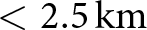
Our results provide empirical evidence for drainage cascades in northeast Greenland, consistent with the mechanism proposed for West Greenland where rapid drainage of one lake can trigger near-synchronous drainage of neighbouring lakes through elastic stress transfer and changes in basal water pressure (Doyle and others, Reference Doyle2013; Christoffersen and others, Reference Christoffersen, Bougamont, Hubbard, Doyle, Grigsby and Pettersson2018). In the northeast Greenland sub-basin, cascades are generally small and spatially compact and most clusters consist of 2-3 lakes with spatial extents typically  $ \lt $2.5 km. This contrasts with some West Greenland examples where cascades can involve larger numbers of lakes over greater distances in regions with very dense lake coverage (Christoffersen and others, Reference Christoffersen, Bougamont, Hubbard, Doyle, Grigsby and Pettersson2018; Chudley and others, Reference Chudley, Christoffersen, Doyle, Abellan and Snooke2019). The predominance of small clusters in our study likely reflects the sparser lake distribution on 79N and Zachariæ Isstrøm which limits the number of lakes that are both close enough and sufficiently full to participate in a given cascade.
Cascade participation among rapid drainage events decreased from 31% in 2019 (107 events in 49 clusters) to 20% in 2020 (39 events in 17 clusters). This reduction is consistent with the overall decline in rapid drainage counts and with the shorter, cooler melt season in 2020. In 2019, sustained above-freezing conditions over a longer period with early onset likely allowed more neighbouring lakes to approach their critical depths at similar times, increasing the chance that a single drainage could trigger additional events nearby. In 2020, with lake levels evolving more variably in time and lake areas remaining smaller, rapid drainages were more often isolated in both space and time, and fewer met the spatial and temporal proximity criteria used to define cascades. The weekly correlation between maximum air temperature and cascade frequency was stronger in 2019 than in 2020, but remained moderate overall (mean  $R^2 \approx 0.57$ vs. 0.33) (Fig. S4b). This indicates that while warmer weeks tend to coincide with more cascades especially in the warmer year, surface temperature alone does not control cascade timing. This is in line with process-based studies that highlight the importance of pre-existing crevasse fields, basal drainage connectivity and the detailed sequence of individual drainage events in governing when cascades are triggered (Christoffersen and others, Reference Christoffersen, Bougamont, Hubbard, Doyle, Grigsby and Pettersson2018; Hoffman and others, Reference Hoffman2018; Chudley and others, Reference Chudley, Christoffersen, Doyle, Abellan and Snooke2019; Reference Chudley and Howat2025).
The signal observed at  $ \gt $1000 m elevation range is different in character. Seasonal mean speeds at this elevation were nearly identical between years (2019: 0.23 m/day; 2020: 0.23 m/day;
 $\Delta = -2.6\%$), and inter-week differences were generally small (
 $ \lt $25%) (Fig. S5). But we observed an anomalous spike in 2020 during the week 17-23 Aug (faster by 63%) and in 2019, a spike during the week of 27 Jul-02 Aug (0.57 vs. 0.2 m/day). This may reflect localized stress responses rather than a sustained regime difference, and should be interpreted with caution given the limited pixel coverage in this region, as there is limited correlation between the image pairs for those dates. The absence of a systematic velocity difference at
 $ \gt $1000 m elevation range therefore suggests that the higher fractional occurrence of cascades at this elevation in 2020 (33% of all clusters vs. 14% in 2019) cannot be attributed to a sustained change in the large-scale extensional stress field, rather it likely reflects the suppression of low-elevation higher activity as described above, combined with the possibility that the late-August velocity pulse may have episodically promoted fracture propagation in deeper inland basins.
The observed cascade locations exhibited a clear topographic control between years. In 2019, cascades were concentrated at lower and mid-elevations, with 77% of all clusters below 800 m and 35% of clusters at  $ \lt $400 m on moderate slopes (0.3–1
 $^\circ$). In 2020, the overall distribution of cascades was only 8% of clusters below 400 m and 64% above 800 m elevation ranges (31% at 800-1000 m; 33% at
 $ \gt $1000 m). In absolute cluster number terms, cascade clusters below 400 m elevation range fell from 17 (2019) to 1 (2020), while clusters above 800 m elevation range declined only marginally from 12 to 11. The higher fractional occurrence of cascades at elevated terrain in 2020 is therefore driven predominantly by a near-total suppression of low-elevation cascading activity, rather than by any meaningful increase in high-elevation cascade frequency. This suppression at low elevations in 2020 is consistent with the velocity observation (Fig. S5). Median surface ice velocities below 400 m elevation range were 21% lower in early June 2020 compared to 2019, and this deficit persisted in the majority of drainage weeks throughout the season. Lower ice velocity could imply reduced tensile strain rates at low elevation, and thus a weaker background extensional stress field within which cascade-triggering fractures must propagate. Under these conditions, the elastic stress perturbation generated by an individual rapid drainage would be less likely to reach the fracture propagation threshold (Christoffersen and others, Reference Christoffersen, Bougamont, Hubbard, Doyle, Grigsby and Pettersson2018; Chudley and others, Reference Chudley2022). Conversely, at 800–1000 m elevation range, where 2020 velocity exceeded 2019 values by 14.3-15.6% through late July and early August (Weeks of 27 Jul-09 Aug), with the seasonal mean 11.6% higher in 2020 (0.92 vs. 0.81 m/day). This increase in velocity in 2020 could imply a relatively more extensional background stress regime at this elevation range, which would lower the fracture propagation threshold in adjacent lake basins and is causing to maintain an equal number as 2019 at 800-1000 m in 2020. For the elevation range
 $ \gt $1000 m the observed velocity in 2020 was faster by 63% (week of 17-23 Aug: 0.587 vs. 0.215 m/day) even though it does not fully resolve the show up of 6 new cluster participation above
 $ \gt $1000 m elevation range in 2020, and should be interpreted with caution given the limited pixel coverage in this bin for those dates due to the lesser correlation. Williamson and others (Reference Williamson, Banwell, Willis and Arnold2018) found no robust critical lake depth or volume threshold for rapid drainage in West Greenland, noting that cascading events break simple statistical relationships between individual lake properties and drainage probability. Our results suggest that the local ice-flow and a further derived strain-rate may represent a key additional control determining whether an isolated rapid drainage escalates into a cascade, a hypothesis that could be tested explicitly using coupled ice-flow and hydrofracture models.
Conclusions
This study characterizes the evolution of supraglacial lakes and rapid drainage cascades on the northeast Greenland Ice Stream during two contrasting melt seasons, 2019 and 2020. Within this 2 year record, the results indicate that the timing and continuity of above-freezing air temperatures with the cumulative PDDs influence supraglacial lake growth, persistence and drainage behaviour. In 2019, a longer period of sustained positive temperatures allowed lakes to expand laterally leading to larger total lake area and more frequent rapid drainage events. In contrast, the shorter and more temporally compressed melt season in 2020 produced a similar number of lakes but with systematically smaller areas and fewer rapid drainages.
Topography further modulated these responses. The 800-1000 m elevation band emerged as a key storage zone, consistently hosting the largest numbers of lakes and intermediate depths, reflecting a balance between limited firn infiltration at higher elevations and the early development of efficient drainage pathways at lower elevations. Surface slope imposed an additional control as gentle slopes ( $ \lt $0.3
 $^\circ$) hosted many, generally shallow lakes and stored the largest total water volume, whereas steep slopes (
 $ \gt $1
 $^\circ$) supported fewer but deeper lakes. Rapid drainage events were more common on gentle slopes, suggesting that where meltwater supply is more limited, flat terrain provides favourable conditions for lakes to reach and maintain the depths required for rapid drainage, while steeper terrain more efficiently routes meltwater away.
The analysis confirms the presence of drainage cascades, although they are small (typically 2-3 lakes per cluster) and spatially compact (extent up to  $ \lt $2.5 km) compared to cascades reported in denser lake networks elsewhere on the Greenland Ice Sheet. Cascade participation among rapid drainage events decreased from 31% in 2019 to 20% in 2020, consistent with the overall reduction in rapid drainage counts and a shorter melt season. Notably, the spatial redistribution of cascade activity between years from lower elevations in 2019 to higher elevations in 2020 mirrors interannual differences in surface ice velocity, suggesting that the local ice-flow regime and associated tensile strain-rate environment may act as an additional control on cascaded rapid drainage alongside melt forcing. Future research could integrate these topographic thresholds into ice dynamic models to better predict the coupling between surface hydrology and ice flow under increasingly variable climate regimes.
Supplementary material
The supplementary material for this article can be found at https://doi.org/10.1017/jog.2026.10179.
Data availability
The supraglacial lake inventory for the 2019 and 2020 melt seasons over the region of interest generated in this study are available on Zenodo at https://doi.org/10.5281/zenodo.18780056. Sentinel-2 Level-2A imagery is freely accessible via the Copernicus Open Access Hub (https://scihub.copernicus.eu). ArcticDEM products were provided by the Polar Geospatial Center and are available at https://www.pgc.umn.edu/data/arcticdem/ ICESat-2 ATL03 data are distributed by the National Snow and Ice Data Center (NSIDC) at https://nsidc.org/data/atl03. AWS temperature data from the KPC_L station were obtained from the PROMICE database (https://www.promice.org).
Acknowledgements
Gopika Das acknowledges funding from the Space Application Centre, Ahmedabad, ISRO, SAC-STC Project ID: STC0404 and partially acknowledges the scholarship support from the Ministry of Education. The authors thank the Scientific Editor and two anonymous reviewers for their constructive comments, which helped improve the manuscript.

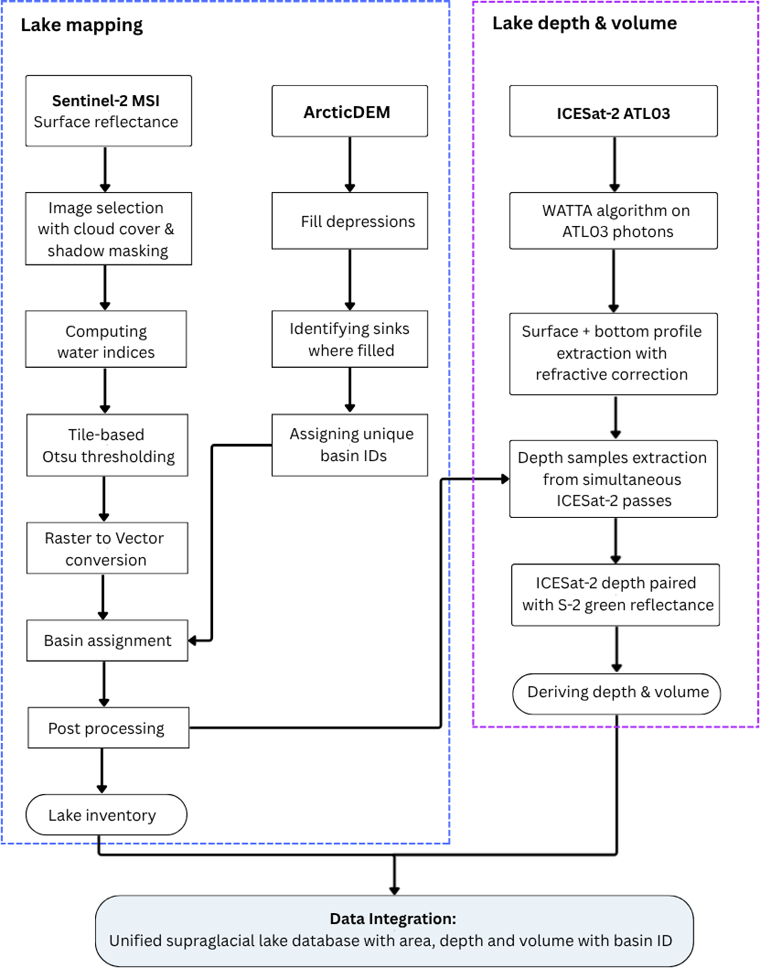
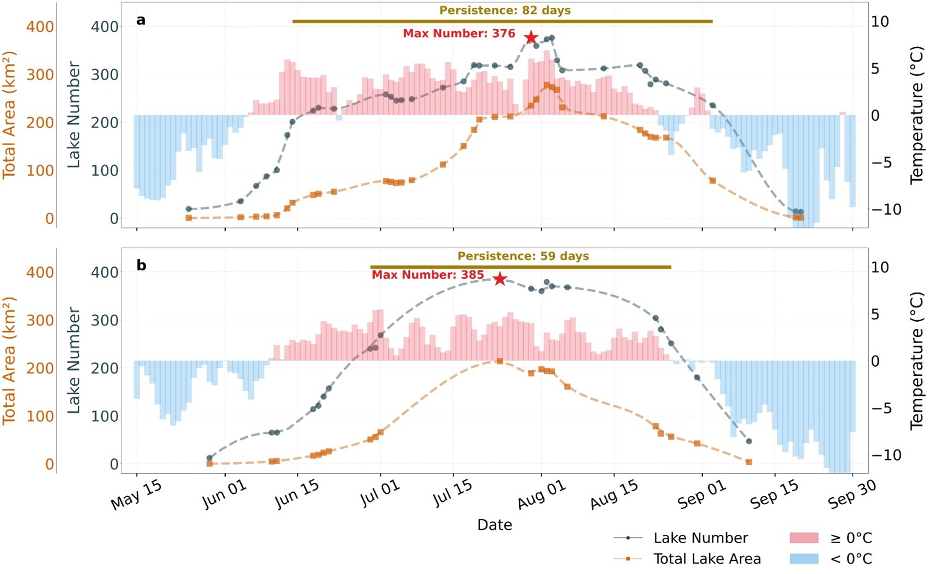


 Open access

