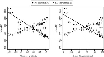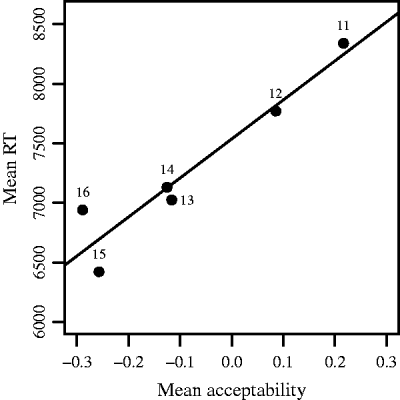


1. Introduction
Introspective judgments of grammaticality have provided a rich source of evidence for syntactic theories of all sorts. Classical introspective judgments classify sentences into two discrete classes, namely grammatical and ungrammatical. Despite their preeminent role in syntactic theorizing, such judgments have come under heavy attack recently. Two prominent points of criticism are, first, that such judgments are not made in a consistent way, and, second, that discrete judgments are not capable of capturing fine grades of grammaticality. This has led to the development of alternative ways of assessing the well-formedness of sentences, chief among them the method of magnitude estimation which allows judgments on a continuous scale (for details see below). We have run three experiments in order to determine how results obtained by the method of magnitude estimation relate to binary grammaticality judgments. Based on the finding of a close correspondence between continuous and binary grammaticality judgments, we present a model which derives binary grammaticality judgments from gradient grammaticality scores.
This paper is organized as follows. In the next section, we discuss the problem of assessing grammaticality and how it has been approached by experimental means. Then, we present our own experiments. Since they use the same sentence materials, we devote a separate section – section 3 – to a description of these materials. The first two experiments are presented in sections 4 and 5 and compared in section 6. The third experiment is presented in section 7. In section 8, we present a model of binary grammaticality judgments. Section 9 presents selected corpus data in order to assess the degree of correspondence between corpus frequencies and degrees of grammaticality as obtained in the preceding experiments. Section 10 contains a summary and final discussion.
2. Assessing grammaticality
A major impetus for the recent interest in alternatives to binary grammaticality judgments derives from a new appreciation of the seeming non-categorical nature of grammaticality. Grammaticality does not seem to be a discrete property; instead, grammaticality appears to form a continuous variable ranging from the completely grammatical to the completely ungrammatical.
As has often been pointed out in the pertinent literature (see in particular Schüze Reference Schütze1996), this idea is not a new one. Especially in the early days of generative grammar, accounting for grades of grammaticality was included among the requirements for an adequate syntactic theory. Later, the notion of degrees of grammaticality found its way into mainstream syntactic theory by making a small number of discrete distinctions instead of a simple binary one. These discrete distinctions are usually represented by symbols like *, ?, ??, ?*. However, as discussed in detail in Bard, Robertson & Sorace (Reference Bard, Robertson and Sorace1996), Schütze (Reference Schütze1996) and Cowart (Reference Cowart1997), the informal use of such diacritics to mark levels of grammaticality is problematic. For example, the exact meaning of symbols like *, ?, ??, ?* has never been defined precisely, and their usage is plagued with inconsistencies.
2.1 Experimental ways of assessing grammaticality
Among the attempts to overcome the problems associated with discrete grammaticality judgments, the method of magnitude estimation (ME) has established itself as a widely used way of obtaining gradient acceptability judgments in an experimentally respectable manner. Magnitude estimation is a well-known method from psychophysics (cf. Stevens Reference Stevens1975). It requires participants to judge physical stimuli (e.g. the length of lines) relative to a reference stimulus. The subject first assigns a numerical value – the so-called modulus – to the reference stimulus. Then, each experimental stimulus is likewise assigned a numerical value, reflecting the perceived ratio between reference and experimental stimulus (e.g. a value of 20 is assigned to a line which is perceived as twice as long as a reference line with a value of 10). Work in psychophysics has shown that people are quite accurate in judging physical stimuli in this way.
When applied to sentence acceptability, the magnitude estimation method works in a similar way: after a reference sentence has been assigned a numerical value, experimental sentences are judged relative to the reference sentence. So far magnitude estimation has been applied to a diverse set of syntactic phenomena, including auxiliary selection in the perfect tense (Sorace Reference Sorace1992, Reference Sorace2000; Bard et al. Reference Bard, Robertson and Sorace1996; Keller & Sorace Reference Keller and Sorace2003), extraction phenomena (Cowart Reference Cowart1997, McDaniel & Cowart Reference McDaniel and Cowart1999, Featherston Reference Featherston2005a, Reference Featherstonc), and word order (Keller Reference Keller, Gleitman and Joshi2000a, Reference Kellerb; Keller & Alexopoulou Reference Keller and Alexopoulou2001).
Magnitude estimation has established itself as a methodologically sound alternative to traditional, discrete grammaticality judgments. It is therefore surprising that little attention has been devoted to the question of how gradient acceptability as measured by magnitude estimation relates to discrete grammaticality judgments, in particular binary judgments classifying sentences simply as grammatical or ungrammatical (but see Weskott & Fanselow Reference Weskott, Fanselow, Featherston and Winkler2009). Clarifying this relationship could be useful in several respects. On the one hand, it could serve as a further validation of the magnitude estimation procedure; in particular, it could contribute to a better understanding of what the numerical values obtained in experiments using this procedure mean. On the other hand, the magnitude estimation literature can easily lead to the impression that discrete grammaticality judgments are practically useless, with the possible exception of the two endpoints of completely grammatical and completely ungrammatical. However, many of the problems that have been pointed out for discrete grammaticality judgments only apply to judgments of individual sentences by individual linguists. The picture may look quite different if discrete grammaticality judgments are obtained in accordance with accepted experimental standards.
Some evidence for this comes from psycholinguistic investigations using the method of speeded grammaticality judgments (SGJ). Experiments of this kind usually work as follows. Participants read sentences which are displayed on a computer screen in a word-by-word fashion. The presentation time for each word is about 300–400 ms; this is long enough to complete all normal comprehension processes like lexical access, syntactic integration, and semantic interpretation, but too short to engage in any kind of deliberate reasoning.Footnote 2 After the last word has been presented, participants have to judge the sentences as either grammatical or ungrammatical as fast as possible (hence the qualification ‘speeded’ in the name of the method). Fast responses are typically ensured by imposing a response deadline of about two seconds. This guarantees that participants give a judgment which is based on their spontaneous first assessment of the grammaticality of the sentence. This method has been used successfully to study the mental processes involved in syntactic ambiguity resolution (e.g. Warner & Glass Reference Warner and Glass1987, Frazier & Flores d'Arcais Reference Frazier and Flores d'Arcais1989, Ferreira & Henderson Reference Ferreira and Henderson1991, Meng & Bader Reference Meng and Bader2000) and in research on second-language acquisition (Hopp Reference Hopp2007).
In our own work using this method – much of which is summarized in Bader & Bayer (Reference Bader and Bayer2006) – we have often included unambiguously grammatical and ungrammatical sentences as controls for syntactically ambiguous sentences. In this way, we have gathered a considerable body of experimental results concerning the perceived grammaticality of various types of syntactic structures. An important lesson we have learned thereby is that a broad range of grammaticality is found when looking at aggregated mean values. That is, while each individual judgment is a binary one – either grammatical or ungrammatical – the mean percentages that result from averaging across participants and sentences are not binary. Such means range from almost 0% to almost 100% with all kinds of values in between. This is true for both sentence tokens and sentence types. For example, two syntactic structures S1 and S2 could both be considered grammatical in the syntactic literature, but nevertheless structure S1 could be judged as grammatical 90% of the time whereas structure S2 might receive an average value of only 75%. Thus, on the level of average means, we can get gradient results even when individual judgments are of a binary nature. In the next section,we discuss the thorny issue of whether such gradient results reflect some kind of gradient grammaticality or something else – for example, differences in acceptability due to the way our performance mechanisms work.
2.2 Grammaticality and acceptability
Not least because of an impressive bulk of research making use of the ME procedure, some consensus has been reached that speakers of a language are able to judge the grammaticality of sentences on a continuous scale (see, among others, the various contributions to Fanselow, Féry, Vogel & Schlesewsky Reference Fanselow, Féry, Vogel and Schlesewsky2006). However, it is one thing to accept the gradience of grammaticality judgments but quite another thing to accept the notion of gradient grammaticality. After all, giving a grammaticality judgment is a mental process which involves more than just the property of grammaticality. According to a distinction which has figured prominently within generative grammar, grammaticality judgments are the joint result of the competence grammar and the performance mechanisms which apply the competence grammar during actual language use. Performance factors, which are usually summarized under the notion of acceptability, include things like memory load and real-world plausibility. From this perspective, grammaticality judgments are just a special way of making use of performance mechanisms. Strictly speaking, the term ‘grammaticality judgment’ is thus a misnomer because grammaticality cannot be judged directly. Judging a sentence always involves more than just the properties that the mental competence grammar ascribes to the sentence. What can be judged in a literal sense is the acceptability of sentences; grammaticality is only one of the factors which determine acceptability (for further discussion, see Chapter 2 of Schütze Reference Schütze1996, and Bard et al. Reference Bard, Robertson and Sorace1996).
What should be concluded from the existence of graded acceptability judgments? One position is to say that the competence grammar makes only discrete distinctions at least a binary one between grammatical and ungrammatical sentences – and that gradience is completely a matter of performance. However, even for someone who subscribes to a sharp distinction between competence and performance this is not a necessary position. The competence-performance distinction in no way precludes grammaticality itself from being a gradient property in addition to the gradience which is brought about by performance mechanisms. Such a position has explicitly been endorsed by Chomsky, as witnessed by the following quotation: ‘Like acceptability, grammaticalness is, no doubt, a matter of degree …, but the scales of grammaticalness and acceptability do not coincide’ (Chomsky Reference Chomsky1965: p. 11). Nowadays, the idea of graded competence is actively pursued in many ways, but especially so in the framework of Optimality Theory, as witnessed by theories like StochasticOptimalityTheory (Boersma & Hayes Reference Boersma and Hayes2001) and LinearOptimalityTheory (Keller Reference Keller2000b), and by researchers who see a close connection between degrees of grammaticality and frequency of usage (see Manning Reference Manning, Bod, Hay and Jannedy2003, for an overview).
Although the distinction between grammaticality and acceptability has a firm place within Generative Grammar, the usefulness of this distinction is not uncontroversial. As pointed out by Featherston (Reference Featherston2005c), the notion of acceptability is as theory-laden as the notion of grammaticality, contrary to what is often assumed (see also Schütze Reference Schütze1996). Furthermore, the distinction between grammaticality and acceptability is an offspring of the distinction between competence and performance, and the latter distinction is considered moot especially by certain kinds of usage-based theories of grammar (see Evans & Green Reference Evans and Green2006 for an overview; for a defense, see Newmeyer Reference Newmeyer2003). In the recent literature concerned with the empirical foundations of linguistic theory, the relevant terminology is not used in a uniform way. Bard et al. (Reference Bard, Robertson and Sorace1996) use the term acceptability only in connection with the perception and judgment of sentence well-formedness, reserving the term grammaticality for properties of the internal competence grammar. Schütze (Reference Schütze1996) notes the same distinction but decides to use acceptability and grammaticality (judgments) interchangeably for pragmatic reasons. Featherston (Reference Featherston2005c) uses the term grammaticality throughout.
Addressing fundamental controversies concerning notions like competence and performance is beyond the scope of the present study. Instead, we pursue the much more modest aim of determining experimentally how judgments obtained through the method of magnitude estimation relate to binary grammaticality judgments. In pursuing this aim, we will use the terms ‘grammaticality’ and ‘acceptability’ in an operationally defined way. In accordance with much of the linguistic literature, we speak of grammaticality judgments when the task explicitly asks people to judge sentences categorically as either grammatical or ungrammatical. For judgments using the method of magnitude estimation, we use the term acceptability judgments. This is again in accordance with much of the literature using this method. Thus, we distinguish between grammaticality and acceptability judgments in a task-dependent way. This is a purely pragmatic decision by which we hope to enhance the readability of this paper. At points where it becomes necessary to have a cover term subsuming acceptability and grammaticality, we will speak of perceived well-formedness.
2.3 Summary
Our experience with the SGJ procedure suggested to us that binary grammaticality judgments might not be so bad after all, if only they were to be obtained according to common experimental standards. To test this hypothesis, this paper first presents two experiments which assess the relationship between continuous acceptability judgments as measured by magnitude estimation and binary grammaticality judgments as obtained by the method of speeded grammaticality judgments. In both experiments, participants had to evaluate sentences using magnitude estimation and speeded grammaticality judgments within the same session. The two experiments share the same experimental materials and differ only in the order of the two experimental procedures: in Experiment 1 the ME procedure preceded the SGJ procedure, whereas the reverse order was used in Experiment 2. It is thus possible to determine whether individual participants give consistent results when using the two methods. Since for this kind of comparison participants have to judge the same sentence materials twice, memory-based repetition effects cannot be excluded. This problem can be overcome by comparing the ME part of Experiment 1 with the SGJ part of Experiment 2. These parts come first in their respective experiments, and accordingly they do not involve any prior encounter with the same experimental materials. This comparison is unaffected by possible repetition effects and therefore allows a stringent assessment of the degree to which the ME and the SGJ method yield convergent results. Because the SGJ method differs from traditional binary grammaticality judgments in requiring timed responses, we ran a third experiment in which participants gave binary grammaticality judgments by filling out a questionnaire without time pressure.
The main finding of our experiments is that the different methods lead to highly similar results, whether the comparison is within or across experiments. This finding naturally raises the question of how gradient and binary judgments are related to each other in terms of the mental representations and processes underlying each type of judgment. As a step toward answering this question, we apply Signal Detection Theory (Green & Swets Reference Green and Swets1966) to arrive at a model of how binary grammaticality judgments are derived from the gradient perception of acceptability which underlies the judgments in an ME experiment.
3. The syntactic structures investigated in Experiments 1 and 2
The sentence materials for the upcoming experiments are made up of three subexperiments. Since the experiments do not differ with regard to the sentence materials but only with regard to the experimental procedure, we give a detailed description of the three subexperiments in this section. For all three subexperiments, results from prior experiments using the method of speeded grammaticality judgments were already known. It was therefore possible to select the experimental materials in accordance with the following a priori requirements. First of all, the experimental conditions should range from completely grammatical to completely ungrammatical in order to determine the relationship between the two methods under consideration across the whole range of grammaticality. At the same time, the experimental conditions should also subsume some subtle distinctions in order to test whether the two methods can detect the same fine details. The final requirement was related to frequency of usage. Since the notion of a relationship between degrees of acceptability and corpus-based frequencies has gained some prominence in recent discussions of the nature of the mental grammar, an additional requirement was that the experimental materials should allow us to address this question based on existing corpus data. We next describe each subexperiment in detail and point out how they jointly meet these requirements.
3.1 Subexperiment A: word order and case
The first subexperiment is concerned with the order of subject and object in embedded clauses, either subject before object (SO) or object before subject (OS). One reason for including this subexperiment is that word order has been the topic of several prior ME experiments (e.g. Keller Reference Keller, Gleitman and Joshi2000a). The results for this subexperiment can therefore serve as a point of direct comparison between the existing ME literature and the current study.
In addition to word order, Subexperiment A varies the case of the object, a manipulation which has not been investigated in prior ME experiments. The object is either an accusative or a dative object. Sample sentences illustrating the manipulation of order and case are shown in (1) and (2). The embedded clauses in (1) contain an accusative object which follows the subject in (1a) and precedes it in (1b). The sentences in (2) are parallel but contain a dative object instead of an accusative object.
(1) Sentences with accusative object
(a) Ich glaube, dass der Pfarrer den Schüler unterstützt hat. I believe that the minister the.acc student supported has
(b) Ich glaube, dass den Schüler der Pfarrer unterstützt hat. I believe that the.acc student the minister supported has ‘I believe that the minister supported the student.’
(2) Sentences with dative object
(a) Ich glaube, dass der Pfarrer dem Schüler geholfen hat. I believe that the minister the.dat student helped has
(b) Ich glaube, dass dem Schüler der Pfarrer geholfen hat. I believe that the.dat student the minister helped has ‘I believe that the minister helped the student.’
The OS sentences in (1b) and (2b) do not differ in (truth-functional) meaning from their SO counterparts in (1a) and (2a). They differ, however, in information-structural terms. The two SO sentences are compatible with sentence-wide focus, that is, they can be used to answer an all-new question like ‘What happened?’. Additionally, they can be used to answer questions asking either for the subject alone (‘Who supported/helped the student?’) or for the object alone (‘Who did the minister support/help?’); they are thus also compatible with narrow focus on either subject or object. The two OS sentences, in contrast, allow only narrow focus on the subject. This difference between SO and OS sentences is among the reasons why SO is considered to be the canonical order of subject and object in German. However, although SO is normally the unmarked order of subject and object, this is not always so. As will be discussed below, whether a given sentence allows broad focus with SO or OS order depends on properties of the verb and its arguments. In the first subexperiment, all sentences contain an animate agent subject and an animate object which is a benefactive or a patient. For this configuration, only SO order licenses broad focus whereas OS order is restricted to narrow focus on the subject. This is independent of the case of the object. A different configuration will be considered in the next subexperiment. In the following, we refer to OS sentences which are only licit under narrow subject focus as discourse-licensed OS sentences.Footnote 3
Sentences with different orders among subject and object have figured prominently in ME as well as in SGJ studies, but have so far not been investigated with both methods in a single experiment. Sentences similar to the sentences with accusative object in (1) were included in the ME experiment reported in Keller (Reference Keller, Gleitman and Joshi2000a) (see also Keller Reference Keller2000b, and Keller & Alexopoulou Reference Keller and Alexopoulou2001). The results of Keller (Reference Keller, Gleitman and Joshi2000a) revealed lower acceptability scores for sentences with OS order than for sentences with SO order. This was true when the experimental sentences were presented without context but also when they were preceded by a context question inducing narrow focus on the subject. With online methods (including self-paced reading and event-related potentials), in contrast, it has been found that a preceding context can remove the disadvantage of OS sentences (see Meng, Bader & Bayer Reference Meng, Bader, Bayer, Wachsmuth and Jung1999, Bornkessel & Schlesewsky Reference Bornkessel and Schlesewsky2006b, Hopp Reference Hopp2007).
Prior experiments using an SGJ procedure to investigate SO and OS sentences like those above have also found a disadvantage for sentences with OS order and no preceding context (e.g. Meng et al. Reference Meng, Bader, Bayer, Wachsmuth and Jung1999, Hopp Reference Hopp2007). Furthermore, Bader & Häussler (Reference Bader and Häussler2006) found that OS sentences with an accusative object were consistently judged worse than OS sentences with a dative object; for SO sentences, in contrast, the case of the object had no effect. Case effects of this kind, which have not been the target of ME experiments as far as we know, seem unexpected from a purely linguistic point of view and might instead be a mere parsing effect. We therefore include case as a second factor within this subexperiment in order to determine whether the disadvantage of accusative OS sentences also shows up when probed with an ME procedure.
For Subexperiment A, 24 sentences were created, with each sentence appearing in four versions according to the two factors Order (SO vs. OS) and Case (accusative vs. dative). All sentences followed the pattern shown in (1) and (2). The 24 sentence quadruples were distributed onto four experimental lists according to a Latin square design. Each experimental list contained only one version of each sentence, with an equal number of sentences occurring in each of the four experimental conditions. This ensures that (i) each participant judges each sentence only once, and (ii) each participant judges the same number of sentences within each experimental condition.
3.2 Subexperiment B: argument alternations
The topic of our second subexperiment is the grammaticality of two types of argument alternations found with German ditransitive verbs. Consider first sentence (3) which contains the ditransitive verb schenken ‘to present’ within the embedded clause.
(3) Ich weiß, dass der Onkel (dem Bub) einen Ring geschenkt hat. I know that the.nom uncle the.dat boy a.acc ring presented has ‘I know that the uncle presented a ring (to the boy).’
Sentence (3) is typical of sentences with ditransitive verbs in three ways. First, subject and dative object are instantiated by animate NPs whereas the accusative object is instantiated by an inanimate NP. Second, the three arguments of schenken appear in the order ‘subject before dative object before accusative object’. Third, the dative object, which is included in parentheses in (3), is an optional argument.
The order of the three arguments of schenken reflects two semantic constraints on argument linearization (cf. Siewierska Reference Siewierska, Jacobs, Stechow, Sternefeld and Vennemann1993 and references cited there). The Animacy Constraint (‘An animate NP precedes an inanimate NP’) causes the accusative argument to appear last; the Agent Constraint (‘An agent NP precedes all other NPs’) puts the subject in initial position. What holds for the verb schenken in (3) holds for the great majority of German ditransitive verbs, including all verbs used in the current subexperiment.
The result of putting sentence (3) into the passive voice is shown in (4).
(4) … dass dem Bub (vom Onkel) ein Ring geschenkt wurde. that the.dat boy by-the uncle a.nom ring presented was ‘…that a ring was presented to the boy (by the uncle).’
Sentence (4) exhibits the effects expected from passivization: first, suppression of the former subject which can optionally appear as a von-PP (corresponding to an English by-PP); second, promotion of the former accusative object to subject, as witnessed by the morphological change from einen Ring (accusative) to ein Ring (nominative). Note that promoting the former accusative object to the grammatical subject function is not accompanied by any corresponding change in word order except the position of the optional by-phrase realizing the former subject. In a sentence with a passivized ditransitive verb, the word order allowing broad sentence focus is ‘dative object before subject’. Since sentences of this kind have an animate dative object together with an inanimate subject (=the former accusative object), we can conclude that in German semantic constraints on argument linearization outrank syntactic constraints. In the following, we refer to OS sentences of this kind as lexically licensed OS sentences.
As mentioned in the preceding section, converging evidence from ME and SGJ experiments shows that discourse-licensed OS sentences like (1b) are perceived as less acceptable than corresponding SO sentences. For lexically licensed OS sentences as in (4), only SGJ data seem to exist (e.g. Bader & Bayer Reference Bader and Bayer2006). These data show that lexically licensed OS sentences do not differ from corresponding SO sentences in terms of perceived grammaticality. This would be compatible with the hypothesis that sentences with OS order are perceived as less than fully well-formed only when they are associated with a marked information structure. By including both lexically licensed OS sentences (Subexperiment B) and discourse-licensed OS sentences (Subexperiment A), and by obtaining ME as well as SGJ data, this hypothesis can be tested in a stringent way.
In addition to the regular passive illustrated in (4), ditransitive verbs in German can undergo the so-called recipient passive as illustrated in (5).
(5) … dass der Bub (vom Onkel) einen Ring geschenkt bekam. that the.nom boy by-the uncle a.acc ring presented got ‘…that the boy was presented a ring (by the uncle).’
The recipient passive is formed with the verb bekommen ‘to get’. It differs from the regular passive in two important ways. First, instead of the accusative object it is the dative object which is promoted to subject when forming the recipient passive. The accusative object is not affected and therefore remains an accusative object. Second, the recipient passive is subject to much tighter semantic constraints than the regular passive. To a first approximation, we can say that the original meaning of bekommen ‘to get’ is still visible in a sentence exhibiting the recipient passive. The dative object that is promoted to subject must accordingly be a recipient of some sort, matching the recipient role of the subject of bekommen. An example illustrating the differential sensitivity of regular passive and recipient passive with regard to semantic constraints is shown in (6).
- (6)
(a) Ich weiß, dass dem Mann ein Buch gestohlen wurde. I know that the man a book stolen was ‘I know that the man was stolen a book.’
(b) ?Ich weiß, dass der Mann ein Buch gestohlen bekam. I know that the man a book stolen got ‘I know that the man was stolen a book.’
The dative object of the ditransitive verb stehlen ‘to steal’ is not a recipient in the narrow sense of someone receiving something. Instead, in an act of stealing something is taken away from someone. For this verb, the recipient passive is accordingly marginal whereas the regular passive is fully acceptable.
While the contrast between examples (5) and (6) is suggestive, the recipient constraint on the formation of the recipient passive is nevertheless only a first approximation. For example, ditransitive verbs without a recipient can often form the recipient passive when some form of inalienable possession is involved. This is illustrated in (7).
(7) Ich weiß, dass der Mann einen Zahn gezogen bekam. I know that the man a tooth pulled got ‘I know that the man was pulled a tooth.’
Sentence (7) is similar to sentence (6b) insofar as the referent of the subject NP (corresponding to the original dative object) does not receive anything but has something removed. Despite this similarity, (6b) is of questionable acceptability whereas sentence (7) is impeccable. A comprehensive discussion of the relevant data, which are clearly much more complex than indicated here, can be found in Leirbukt (Reference Leirbukt1997). Furthermore, it is a controversial issue whether the recipient passive is a true passive-like operation on a par with the regular passive (see Eisenberg Reference Eisenberg2004 for discussion and references). It is not necessary for our purposes to take a stance in this discussion.
Important for us is the fact that the second subexperiment complements the first one in several respects. First, regular passivization creates lexically licensed OS sentences which allow sentence-wide focus and thereby differ crucially from the discourse-licensed OS sentences of the first subexperiment, which require narrow focus on the subject. Second, prior SGJ results (Bader & Bayer Reference Bader and Bayer2006, Häussler & Bader Reference Bader and Bayer2006) lead us to expect that neither of the conditions investigated in Subexperiment B should give rise to strong feelings of unacceptability. This subexperiment therefore allows us to assess the degree to which the ME and the SGJ method can reveal subtle acceptability distinctions. Finally, for sentences in the recipient passive condition, Häussler & Bader (Reference Bader and Bayer2006) have found a correlation between judgment data and verb-based corpus frequencies. Including Subexperiment B within the current study makes it possible to test whether the two methods are equally sensitive with regard to lexical frequency.
For Subexperiment B, 42 sentences were taken from the larger study of Häussler & Bader (Reference Bader and Bayer2006). Each sentence appeared in the six conditions resulting from crossing the two factors Linking (active vs. regular passive vs. recipient passive) and Number of Arguments (two vs. three). All sentences were constructed on the pattern shown by the examples in (3) (active), (4) (regular passive) and (5) (recipient passive). The phrase that is given in parentheses in these examples was included in the condition ‘Number of Arguments=three’ and excluded in the condition ‘Number of Arguments=two’. Each sentence contained a different ditransitive verb; frequency information for the set of verbs is provided in section 9. The 42 sentence sextets were distributed over six experimental lists, again following a Latin square design (see description for Subexperiment A).
3.3 Subexperiment C: verb-cluster linearization
The third and final subexperiment investigates the linearization of verbs when several of them occur together in clause-final position, forming a so-called verb cluster (for further discussion, see Wurmbrand Reference Wurmbrand, Everaert and Riemsdijk2006). Reflecting the verb-final nature of German, a selected verb normally precedes a selecting verb, giving rise to the kind of nested orders shown for the case of three-verb clusters in (8a). Here and in the following, we follow a common practice and number the verbs of a verb cluster beginning with the highest verb, which is assigned 1. In turn, the verb selected by verb 1 is assigned 2, and so on.
- (8)
(a) [… V3←V2←V1 ]CP – order 3–2–1
(b) [… Aux1→V3←Mod2]CP – order 1–3–2
There are some exceptions to this pattern, however. In particular, when a modal verb is in the perfect tense, the perfect auxiliary has to appear in initial position according to prescriptive grammars of German, giving rise to the pattern in (8b). An example instantiating this pattern is shown in (9).
(9) Ich weiß, dass Kai das Buch [hat1 kaufen3 müssen2]. – order 1–3–2 I know that K. the book has buy must ‘I know that Kai had to buy the book.’
Since there are six different permutations of a cluster with three elements, this implies that five of them are ungrammatical in Standard German. To ease later reference, the six possible permutations are summarized in (10) according to two dimensions: the order of verb and modal (‘V before Mod’ versus ‘Mod before V’) and the position of the auxiliary (first versus second versus third). The Standard German order, which is printed in boldface in table (10), has ‘V before Mod’ and ‘Aux=1’.
(10)

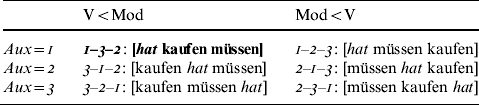
Bader & Schmid (Reference Bader and Schmid2009) used the method of speeded grammaticality judgments in a comprehensive investigation of auxiliary inversion in verb clusters with modal verbs. This investigation has shown that the Standard German order 1–3–2 consistently receives the highest percentages of ‘grammatical’ judgments. However, the remaining five orders, although all banned by prescriptive grammar, are not all judged equally bad. Most strikingly, the order 3–1–2 in which, as in Standard German, the auxiliary has been inverted, although only partially, was judged only 10–20% worse than the Standard German order 1–3–2. Because auxiliary inversion in verb clusters is known to involve a large amount of dialectal variation (see Schmid & Vogel Reference Schmid and Vogel2004), Bader & Schmid (Reference Bader and Schmid2009) also looked at the regional background of their participants. Since the pattern of well-formedness just described was found to be independent of participants' regional background, Bader & Schmid (Reference Bader and Schmid2009) concluded that the order 3–1–2 is an optional variant in Colloquial German although not in Standard German. The remaining four orders received rather low judgments but still showed certain gradations which will be discussed later. At this point, we only note that two orders (2–1–3 and 2–3–1) were rejected almost completely. Thus, the six conditions of the verb cluster subexperiment span the whole range from fully acceptable to fully unacceptable, with further gradations in between.
Wurmbrand (Reference Wurmbrand, Burelle and Somesfalean2004) claims that the order 3–1–2 is licit only if the lexical verb is narrowly focused (see also Schmid & Vogel Reference Schmid and Vogel2004). However, experimental investigations of this issue have not in fact revealed any focus-related effects on verb-cluster linearization. This is true both for experiments with written sentence presentation and manipulation of focus by the use of focus particles (Bader & Schmid Reference Bader and Schmid2009), and for experiments with auditory sentence presentation in which focus was manipulated by intonational means (Bader & Henninger in preparation). Verb-cluster linearization thus seems to be independent of the sentence's information structure (see also Sapp Reference Sapp2006).
In summary, the serialization of verbs is of particular interest because it contrasts in important ways from the serialization of subject and object as discussed in the preceding section. First of all, as just pointed out, the six different permutations of a three-verb cluster span the whole range from the completely grammatical to the completely ungrammatical. A second difference concerns the status of the possible linearization patterns within the grammar. With regard to the linearization of subject and object, both orders are considered to be grammatical, but – as discussed above – they may differ in terms of information-structural markedness depending on features of the particular verb and its arguments. For the linearization of verbs within a verb cluster, in contrast, information-structural properties do not seem to be involved. Instead, certain orders are grammatical while others are ungrammatical, independent of any particular discourse context. Since some researchers have ascribed a key role to information-structural markedness in phenomena of gradient well-formedness (e.g. Sorace & Keller Reference Sorace and Keller2005), Subexperiment C provides a valuable contrast to the first two subexperiments.
The materials for Subexperiment C was taken from Experiment 1 of Bader & Schmid (Reference Bader and Schmid2009). It consisted of 30 sentences, each appearing in six versions according to the factors Verb–Modal Order (V<Mod vs. Mod<V) and Auxiliary-Position (First vs. Second vs. Third). All sentences adhered to the model established by example sentence (9). The six versions of each sentence differed only with respect to the order of the three verbs in the clause-final verbcluster, as shown in (10). The 30 sentence sextets were again evenly distributed over six experimental lists following a Latin square design.
3.4 Summary of experimental material
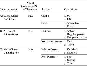
Overall, the three experiments that we report below tested 96 experimental sentences representing 16 different syntactic conditions, grouped into three subexperiments. Table 1 summarizes the number of conditions and sentences in each subexperiment.
Overview of the three subexperiments that together constitute the experimental materials for the three experiments reported in this paper.

The sentence lists of the individual subexperiments were combined into twelve experimental lists (twelve being the least common multiple of four and six). Each experimental list contained 96 sentences. Across the twelve experimental lists, the four lists of Subexperiment A were repeated three times and the six lists of Subexperiments B and C two times. Each experimental list was combined with the same list of 18 filler sentences. These filler sentences represented a variety of grammatical and ungrammatical sentence structures, including several sentences violating subject-verb agreement.
4. Experiment 1
Experiments 1 and 2 investigated the sentence materials described in the preceding section by means of two procedures: an ME and an SGJ procedure. In Experiment 1, participants first judged sentences using the ME procedure. Directly thereafter, they judged the same sentences by means of the SGJ procedure. In Experiment 2, the order of the two procedures was reversed.
4.1 Method
4.1.1 Participants
Twenty-four students at the University of Konstanz participated in Experiment 1. All were native speakers of German and were naive with respect to the purpose of the experiment. Participants were either paid or received course credit for participation in the experiment.
4.1.2 Materials
The sentence materials for Experiment 1 consisted of the three subexperiments that were described in the preceding section (cf. table 1), plus the filler sentences also described there. For each participant, one of the twelve experimental lists described above was selected. This list was presented twice, a first time for the ME part and a second time for the SGJ part of Experiment 1. Thus, all participants gave two judgments for each sentence. For each participant, the experimental list was randomized separately for the ME and the SGJ part.
4.1.3 Procedure
All participants were tested in separate sessions at the psycholinguistics lab of the University of Konstanz. Each session lasted between 50–60 minutes; the two parts – ME and SGJ – took about the same amount of time.
4.1.3.1 Magnitude estimation
The ME procedure that we used in our experiments closely follows the description of the ME method in Bard et al. (Reference Bard, Robertson and Sorace1996), Sorace (Reference Sorace2000), and Keller (Reference Keller2000b). The ME part of each experimental session consisted of three phases which were run using software developed in our lab. In the customization phase, participants were acquainted with the principles of ME by judging the length of six lines presented on a computer screen. In the training phase, they judged the acceptability of ten training sentences. In the final experimental phase, they judged the acceptability of the experimental and filler sentences described in the materials section.
Each phase consisted of the following steps. First, participants read an instruction that was displayed on the computer screen. The instruction explained the ME procedure with the help of an example. At the end, the main points were repeated in the form of a list. Participants were encouraged to contact the experimenter (who was always present in the lab) in case there were any questions regarding the task.
When participants had finished reading the instruction, they pressed a button which triggered the display of the reference stimulus (either a line or a sentence). Participants assigned a numerical value to the reference stimulus. Afterwards, the experimental stimuli were displayed one by one, and participants judged each stimulus relative to the reference stimulus. The reference stimulus as well as the modulus value assigned to it remained visible on the computer screen while participants worked through the experimental stimuli. Participants typed their judgments using a regular keyboard. Judgments and judgment times were recorded automatically.
To enhance comparability with prior work, the reference sentence for the final experimental phase was taken almost literally from Keller (Reference Keller2000b; sentence (B.18)/page 377). As shown in (11), the reference sentence is a sentence with discourse-licensed OS word order. It is thus similar to the OS sentences in Subexperiment A except that the object is filled by an inanimate NP in the reference sentence whereas Subexperiment A contains only animate NPs.
(11) Ich glaube, dass den Bericht der Chef in seinem Büro gelesen hat. I believe that the.acc report the.nom boss in his office read has ‘I believe that the boss read the report in his office.’
4.1.3.2 Speeded grammaticality judgments
The SGJ part of our experiments was run using the DMDX software developed by K.I. Forster and J.C. Forster at Monash University and the University of Arizona. Each trial began with the presentation of the words ‘Bitte Leertaste drücken’ (‘Please press spacebar’). After the spacebar was pushed, a fixation point appeared in the center of the screen for 1050 ms. Thereafter, the sentence was presented in a word-by-word fashion with each word appearing successively in the center of the screen. The presentation time for each word was 225 ms plus an additional 25 ms per character. There was no interval between words. Immediately after the last word, three question marks appeared on the screen, indicating to participants that they now had to judge the grammaticality of the sentence. Participants had to give their answer by pressing the right shift key to judge a sentence as grammatical and the left shift key to judge a sentence as ungrammatical. Type of response and response time were recorded automatically. If a participant did not make a response within 2000 ms, the words ‘zu langsam’ (‘too slow’) appeared on the screen and the trial was aborted. Each participant received 10 practice items before the experimental session started. The reference sentence of the prior ME part (cf. (11)) was always presented as the first sentence of the experimental session.
4.2 Scoring
Following standard practice, we computed three different measures for the SGJ part of Experiment 1: the percentages of ‘grammatical’ judgments, the reaction times for giving a ‘grammatical’ judgment, and the reaction times for giving an ‘ungrammatical’ judgment. All trials that were aborted because participants did not respond within the given time limit were removed prior to all data analyses. This affected less than 1.5% of the data. Since the main information is provided by the percentages of ‘grammatical’ judgments, we present only the percentages in this section. Reaction time results are presented and analyzed in Appendix A and Appendix B.
Computing the results for an ME experiment is somewhat more involved because the numerical scores that participants assign to the experimental sentences can only be interpreted in relation to the modulus value that each participant gives to the reference sentence at the beginning of the experiment. For example, if an experimental sentence is assigned a value of 100, the meaning of this value is very different depending on whether the initial reference sentence received a modulus value of 50 (in which case the experimental sentence was judged as being twice as good as the reference sentence) or a modulus value of 200 (in which case the experimental sentence was judged as only half as good as the reference sentence). The raw judgments obtained in an ME experiment therefore have to be transformed in such a way that the value assigned to the reference sentence is taken into account.
In the following, we make use of a commonly used transformation which scales the individual scores of each participant directly in relation to the participant's modulus value. This is achieved by dividing the score assigned to each experimental sentence by the value assigned to the reference sentence. The resulting ratio is further transformed by taking the logarithm to the base ten (cf. Bard et al. Reference Bard, Robertson and Sorace1996).Footnote 4
4.3 Results
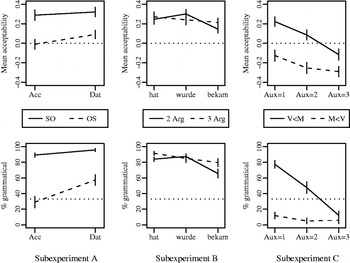
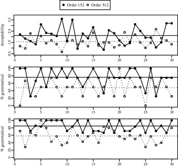
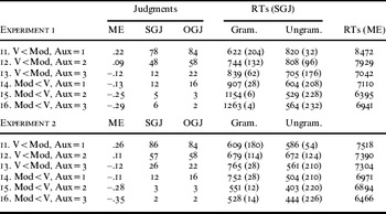
Figure 1 shows the results for both the ME and the SGJ parts of Experiment 1 (see Appendix A for the exact numerical values).Footnote 5 The mean judgments for the reference sentence in (11) are indicated by the dotted lines in figure 1. In an ME experiment, the reference sentence necessarily receives an acceptability score of 0 due to the way in which results are computed. In the SGJ part of Experiment 1, the reference sentence was judged as grammatical 33% of the time. Figure 1 reveals that all experimental conditions that are above the reference sentence in the ME part of Experiment 1 are also above the reference sentence in the SGJ part; the same is true for conditions below the reference sentence.
ME (upper row) and SGJ (lower row) results for the three subexperiments of Experiment 1. The horizontal dotted lines represent the mean judgments given to the reference sentence. The vertical lines represent standard errors by participants.

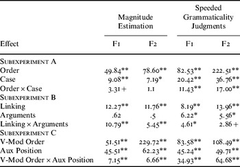
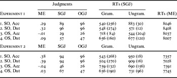
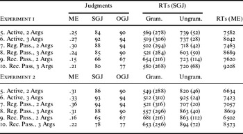
We first discuss the three subexperiments separately and then compare the ME and the SGJ method taking all three subexperiments into account. Each pairing of experimental procedure and subexperiment was subjected to two analyses of variance (ANOVA), with either participants (F1) or items (F2) as an additional random factor. The results of all ANOVAs are summarized in table 2.Footnote 6
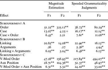
ANOVA results for Experiment 1. F1=analysis by participants; F2=analysis by items. **=p<.01; *=p<.05; +=p<.1.

4.3.1 Subexperiment A: word order and case
As expected from the existing literature on word order variation in German, the factor Order had a significant effect on both ME and SGJ judgments (see table 2 for the exact ANOVA results). Sentences with SO order were judged much better than sentences with OS order. The effect of Case was also significant. Sentences with dative case were judged better than sentences with accusative case. For the SGJ part of Subexperiment A, the effect of Case has to be qualified by a significant interaction between Order and Case. This interaction reflects the finding that for SO sentences, dative sentences were judged non-significantly better than accusative sentences (96% vs. 89%).Footnote 7 For OS sentences, in contrast, dative sentences received significantly higher percentages of ‘grammatical’ judgments than accusative sentences (57% vs. 29%). In the ME results, the same pattern showed up. The difference between dative and accusative sentences was .03 for SO sentences (.29 vs. .32) but .10 for OS sentences (−.01 vs. .09). Nevertheless, the interaction between Order and Case was not significant for the ME part of Subexperiment A.
The results obtained here are comparable to those found by Keller (Reference Keller, Gleitman and Joshi2000a). In Keller's ME study, the acceptability score was 0.38 for SO sentences and 0.11 for OS sentences (as estimated from figure 1 of Keller Reference Keller, Gleitman and Joshi2000a). The respective values obtained in Subexperiment A are .29 and .01. The acceptability scores obtained by Keller are thus somewhat higher than those obtained here; since these values must be interpreted relative to the modulus value assigned to the reference sentence, and since the reference sentence is not reported in Keller (Reference Keller, Gleitman and Joshi2000a), the reason for this discrepancy is unclear. Importantly, however, the distance between SO and OS order is almost the same in Keller's and our experiment (0.27 and 0.29, respectively). When the logarithmic transformation is undone, this means that OS sentences were rated as about half as acceptable as SO sentences in both experiments. We thus conclude that the ME part of Experiment 1 was a successful replication of prior ME studies.
4.3.2 Subexperiment B: argument alternations
The main factor Linking (active vs. regular passive vs. recipient passive) was highly significant in both the ME and the SGJ parts of Subexperiment B. The main factor Number of Arguments, in contrast, was significant in the SGJ part of Subexperiment B but not in the ME part. Importantly, for both procedures the main effects have to be qualified by a significant interaction (marginal in the item analysis of the SGJ results).
One way to understand this interaction is by looking at the effects caused by the number of arguments. Numerically, we see the same pattern for the ME and the SGJ results. For the active and the recipient passive, including all three arguments leads to higher acceptability scores than including only two arguments. For the regular passive, in contrast, the factor Number of Arguments has a reverse effect. Statistically, however, only recipient passive sentences showed a significant difference between two- and three-argument sentences for both experimental procedures (ME: .21 vs. .15; SGJ: 80% vs. 66%). For the SGJ part of Subexperiment B, this was also the only significant difference; for the ME part, Number of Arguments also had a significant effect for regular passive sentences (.24 vs. .30). Given these mixed statistical results, we postpone further discussion to Experiment 2 in order to see how stable the pattern of results is. Correlations between the behavioral results and corpus frequencies obtained for the individual verbs used in Subexperiment B will be presented in section 9.
4.3.3 Subexperiment C: verb-cluster linearization
With both experimental procedures, the Standard German order 1–3–2 was judged best, the non-standard order 3–1–2 was judged second-best, and the remaining four orders received rather low scores – scores in the negative range with the ME procedure, and scores in the range of 5%–12% with the SGJ procedure. Consequently, the two main factors Verb–Modal Order and Auxiliary Position as well as the interaction between them are highly significant in both parts of Subexperiment C.
The significant interaction reflects the finding that auxiliary position has quite different effects depending on the order of main verb and modal verb. When the order of main and modal verb adheres to the regular German order ‘V<Mod’, we see a three-way distinction with large, significant differences between the three auxiliary positions. The order 1–3–2 received higher judgment scores than the order 3–1–2 (ME: .22 vs. .09; SGJ: 78% vs. 48%). The order 3–1–2 was in turn judged much better than the order 3–2–1 (ME: .09 vs. −.12; SGJ: 48% vs. 12%). With the order ‘Mod<V' – the reverse of the regular order of verbs in German – we get only a two-way distinction. The completely inverted order 1–2–3 was judged better than the two remaining orders 2–3–1 and 2–1–3, which did not differ from each other. This pattern can be observed both in the ME and in the SGJ results. It leads to a significant difference in the ME results (−.11 vs. mean of −.25 and −.29) but not in the SGJ results (12% vs. mean of 6% and 5%).
The results found in Subexperiment C are similar to what was found in Experiment 1 of Bader & Schmid (Reference Bader and Schmid2009), although there are some differences in terms of absolute values. Subexperiment C thus adds to the existing body of evidence showing that with regard to the three-verb clusters under consideration, the Standard German order 1–3–2 with complete inversion of the auxiliary is judged best by native speakers. Of the remaining five orders, which are all ungrammatical according to prescriptive grammar, the order 3–1–2 with partial inversion of the auxiliary is also accepted to a considerable degree, but all other orders are largely rejected.
4.3.4 Comparison of ME and SGJ results
A visual inspection of figure 1 reveals a striking resemblance between the results obtained by means of the ME procedure and those obtained by means of the SGJ procedure. In order to assess the similarity quantitatively, we computed the correlation coefficients between ME and SGJ results. This can be done at different levels of granularity. Since each subject judged the very same sentences using both methods, at the most fine-grained level one could compare individual judgments across the two methods. However, this cannot be done by means of simple correlations because ME judgments are given on a continuous ratio scale whereas SGJ judgments are given on a binary nominal scale. How individual judgments can nevertheless be related to each other will be discussed when we introduce our model of grammaticality judgments in section 8.Footnote 8
Since each participant judged several sentences within each syntactic condition, and conversely each sentence was judged by several participants, the next-higher level of granularity was gotten by computing the mean scores for the sixteen syntactic conditions included in Experiment 1 individually for each participant or for each sentence. Finally, at the most general level, the two experimental methods under consideration can be compared on the basis of the 16 grand means depicted in figure 1, that is, the means that result from aggregating across participants and sentences. The table in (12) shows the correlations between ME and SGJ results separately for participant means, sentence means, and grand means.
(12)

The table in (12) shows correlation coefficients which are already substantial when we look at means aggregated over participants or over items. When we look at grand means, the observed correlation shows an almost perfect linear relationship between ME results and SGJ results. The fact that participant means correlate less strongly than sentence means (r=.58 versus r=.79) indicates that there is more variation within the group of participants than within the group of sentences. This variation is present in the ME and the SGJ results in similar ways, as revealed by a linear regression model relating ME results to SGJ results with either participants or sentences as an additional factor. This gives us a model in which the parameters relating the two types of results are estimated separately for each participant or sentence. The model fit in this case is quite similar whether we compare across participants or across sentences: for participant-wise means, R 2=0.75; for sentence-wise means, R 2=0.78.Footnote 9
4.4 Discussion
Experiment 1 assessed sentence well-formedness using an ME and an SGJ procedure and found that the two procedures lead to highly comparable results. Some discrepancies between the two procedures were also visible. Drawing strong conclusions from Experiment 1 would be premature, however. Since participants judged all sentences first with the ME and then with the SGJ procedure, the judgments using the ME procedure might have influenced the later judgments using the SGJ procedure. In order to have the data necessary for an independent comparison of the two procedures, Experiment 2 replicates Experiment 1 but with the order of the two procedures reversed.
5. Experiment 2
In Experiment 2, the SGJ method was administered first and the ME method second. In all other respects, Experiment 2 was identical to Experiment 1.
5.1 Method
5.1.1 Participants
Twenty-four students at the University of Konstanz participated in Experiment 2. None of the participants had taken part in Experiment 1.
5.1.2 Materials and procedure
All materials and the two experimental procedures used in Experiment 2 were the same as in Experiment 1. The only difference with respect to Experiment 1 was that judgments were first given using the SGJ method and then using the ME method.
5.2 Results
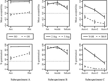
Figure 2 shows the results for Experiment 2. These results were computed in the same way as the results for Experiment 1. The ANOVA results for Experiment 2 are summarized in table 3. The reference sentence was judged as grammatical 17% of the time in the SGJ part of Experiment 2, which is lower than the 33% that the reference sentence received in Experiment 1. A possible reason for this difference might be that the SGJ part was done first in Experiment 2 but second in Experiment 1. Except for the training sentences, the reference sentence was therefore the very first sentence that participants had to judge in Experiment 2, whereas they had already judged all sentences before in Experiment 1 (albeit with a different procedure). In Experiment 1, the reference sentence might therefore have ‘profited’ from the fact that participants were already acquainted with all kinds of more or less degraded sentences.
ME (upper row) and SGJ (lower row) results for the three subexperiments of Experiment 2. The horizontal dotted lines represent the mean judgments given to the reference sentence. The vertical lines represent standard errors by participants.

5.2.1 Subexperiment A: word order and case
The pattern of results that Experiment 2 yielded for Subexperiment A is quite similar to the pattern obtained in Experiment 1. The two main effects of Case and Order were significant with both methods (marginally so for the factor Case in the item analysis of the ME results). As before, the SGJ results show a highly significant interaction between Case and Order. While accusative and dative sentences do not differ in the condition SO (94% for both), a substantial disadvantage for accusative sentences in comparison to dative sentences is visible for sentences with OS order (46% vs. 67%). The ME results show the very same pattern: almost identical acceptability scores for SO sentences but a disadvantage for accusative OS sentences in comparison to dative OS sentences. This time, the interaction is also fully significant in the participant analysis of the ME results but again not significant in the item analysis. We will consider a possible reason for the discrepancy between the ME and SGJ results with regard to the statistical analysis in the final discussion section.
ANOVA results for Experiment 2. F1=analysis by participants; F2=analysis by items. **=p<.01; *=p<.05; +=p<.1.

5.2.2 Subexperiment B: argument alternations
For Subexperiment B on argument alternations, the pattern of results and the statistical analyses also look quite similar across Experiment 1 and Experiment 2. The main effect of Linking as well the interaction between Linking and Number of Arguments were again highly significant both in the ME and the SGJ results. The main effect of Number of Arguments was significant for the SGJ but not for the ME results. Sentences with three arguments received higher judgment scores than sentences with two arguments in the two conditions ‘active’ and ‘recipient passive’; in the condition ‘regular passive’, in contrast, sentences with two arguments were judged better than sentences with three arguments. While this pattern is visible in both the ME and the SGJ results, the statistical analysis gives somewhat varied results. For the recipient passive, the difference between two- and three-argument sentences was significant for the SGJ results and marginally significant for the ME results (ME: .22 vs. .16; SGJ: 78% vs. 64%). All other differences were either marginally significant or not significant at all.
While the differences between two- and three argument sentences are stable across experiments, with the exception of the difference found for the recipient passive they must be considered tentative given the lack of statistical confirmation. For the active sentences, the two-argument versions were derived from the three-argument versions by simply omitting the dative argument. While this is usually possible for ditransitive verbs, some dative arguments may be harder to drop than others, which might explain why two-argument sentences received somewhat lower judgments scores than three-argument sentences (see also Meng & Bader Reference Meng and Bader2000). For the regular and the recipient passive, three-argument sentences are sentences containing the optional by-PP corresponding to the active subject; in two-argument sentences, this PP is missing. In the only difference that was significant throughout, two-argument recipient passive clauses received lower judgment scores than recipient passive clauses with three arguments. Thus, introducing the optional by-PP increases the perceived well-formedness of sentences in the recipient passive. This is just the opposite of the effect found for the regular passive. We do not know why this should be so, and we are not aware of any observations of a similar kind in the syntactic literature. We must therefore leave this as an issue for future research.
5.2.3 Subexperiment C: verb-cluster linearization
For the final subexperiment, Experiment 2 yielded again results quite similar to those found in Experiment 1. The two main factors and the interaction between them were all highly significant both in the ME and in the SGJ results. The reason for this interaction is the same as before. When the main verb precedes the modal verb, a three-way distinction arises: sentences in the condition ‘Aux=1’ are judged substantially better than sentences in the condition ‘Aux=2’ (ME: .26 vs. .11; SGJ: 86% vs. 57%), and sentences in the condition ‘Aux=2’ are in turn judged much better than sentences in the condition ‘Aux=3’ (ME: .11 vs. .12; SGJ: 57% vs. 26%). When the order of main and modal verb is switched and the modal precedes the main verb, in contrast, only a two-way distinction turns up. The two conditions ‘Aux=2’ and ‘Aux=3’ do not differ from each other, while somewhat higher values are obtained in the condition ‘Aux=1’. In Experiment 2, this pattern is statistically confirmed for both the ME and the SGJ results (ME: −.12 vs. mean of −.28 and −.34; SGJ: 12% vs. mean of 3% and 2%).
5.3 Comparison of ME and SGJ results
Figure 2 shows that the two experimental procedures for assessing acceptability again lead to closely corresponding results. The correlations between ME and SGJ at three levels of granularity, namely participant means, sentence means, and grand means, are given in (13).
(13)

The correlation coefficients in (13) are almost identical to those found for Experiment 1 (see (12)). As before, the correlation is almost perfect when considered at the level of grand means. Furthermore, the sentence-wise correlation is again higher than the participant-wise correlation. Thus, the ME and the SGJ procedure lead to highly similar results regardless of which one is administered first.
5.4 Discussion
The results of Experiment 2 confirm those of Experiment 1. Like the preceding experiment, Experiment 2 shows that judging sentences by means of an ME procedure yields results that closely parallel the results obtained with an SGJ procedure. However, the conclusions that the current experiment allows us to draw about the two methods are again limited because the same participants judged the same sentences with both methods in a single experimental session. In order to overcome this limitation, we now turn to a comparison of Experiment 1 and Experiment 2.
6. Comparison of Experiments 1 and 2
The two preceding experiments have revealed a close correspondence between results obtained with the ME method and results obtained with the SGJ method. This clearly demonstrates that native speakers are very consistent when judging the same sentences twice in short succession (c. 30 minutes), even when two quite different judgment procedures are used and independent of the order of the two procedures. However, it cannot be excluded that the second judgment was influenced by a memory representation of the sentence together with its judgment on first encounter.
The table in (14) shows the overall means of all experimental sentences broken down by experiment and procedure, thereby providing a general assessment of the possible effect brought about by the order in which the two experimental procedures were administered.
(14)

The table in (14) shows that Experiments 1 and 2 produced very similar results, with slightly higher scores obtained in Experiment 2. Since this is true for both experimental procedures and thus independent of which procedure was administered first, it seems that the participants in Experiment 2 were slightly more liberal than the participants in Experiment 1. Overall, the order of presentation thus had no effect on perceived acceptability/grammaticality.
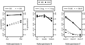
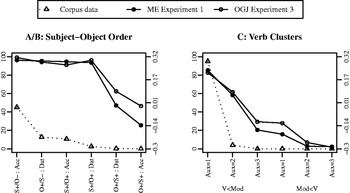
We now compare the ME results from Experiment 1 to the SGJ results from Experiment 2. Since these are the results that were obtained in the first part of each experiment, they are not influenced by any prior encounter with the same sentences. Figure 3 graphically depicts the relevant comparisons separately for each of the three subexperiments. For ease of comparison, ME and SGJ results have been plotted on a single graph. The open circles represent the ME results from Experiment 1 (scale on the left-hand axis). The corresponding SGJ results from Experiment 2 are represented by filled circles (scale on the right-hand axis).
ME and SGJ results plotted on a single graph for each of the three subexperiments (A–C).

Again, we see a very close fit between ME and SGJ results. As before, the quality of the fit was assessed by computing correlations between ME and SGJ results. In addition, we computed the correlations between the ME parts and between the SGJ parts of the two experiments. This gives us an estimation of how stable the results of the two experimental procedures are when the same sentence materials are presented to different groups of native speakers. The resulting correlation coefficients are shown in (15). A correlation across participants could not be computed in this case because the participants in Experiment 1 were different from those of Experiment 2.
(15)
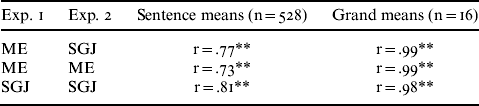
The table in (15) shows that all correlations across the two experiments are quite high when computed for the 528 sentence-wise means, and almost perfect when computed for the grand means of the 16 syntactic conditions. We thus conclude that gradient acceptability judgments obtained by means of the ME procedure are in close correspondence to binary grammaticality judgments gathered with the help of the SGJ procedure.
In the next section, we present a final experiment which obtained binary grammaticality judgments by means of an offline questionnaire.
7. Experiment 3
The two preceding experiments have shown a very close correspondence between continuous, numerical judgments and discrete, binary judgments. While this is an interesting finding by itself, it has to be noted that the way we obtained binary judgments differs in an important way from how such judgments are traditionally obtained. Because we used the method of speeded grammaticality judgments for obtaining binary judgments, participants had to give a quick response which did not leave much time for thinking about the sentences under consideration. This was of course a major reason for using the SGJ procedure in the first place. A rather stringent response deadline was imposed in order to get spontaneous judgments, uncontaminated by deliberate reasoning about, e.g., issues of prescriptive grammar. Since fast presentation rates coupled with quick responses distinguish speeded grammaticality judgments from traditional grammaticality judgments which are not time-limited in any way, we ran a final experiment in which binary grammaticality judgments were obtained by means of an offline questionnaire. Here, participants had as much time as they wanted for reading and judging each sentence. Except for this procedural change, Experiment 3 was identical to the preceding two experiments.
7.1 Method
7.1.1 Participants
Thirty-six students at the University of Konstanz participated in Experiment 3.
7.1.2 Materials and procedure
Experiment 3 used the same sentence materials as the two preceding experiments. Twelve questionnaires were constructed on the basis of the twelve experimental lists that were formed by combining the sentence lists of the individual subexperiments (see subsection 3.4). Each experimental list contained 96 sentences which were interspersed among the same 18 filler sentences used in the prior experiments. In addition, the reference sentence of the ME experiments was added as the first sentence of each questionnaire. The experimental stimuli were randomized differently for each of the twelve questionnaires.
Participants completed the questionnaires as part of a class session. They were asked to judge the grammaticality of each sentence on the questionnaire by marking one of the two options ‘grammatical’ or ‘ungrammatical’ printed beneath each sentence. Participants needed about 20–30 minutes to complete the questionnaire.
7.2 Results
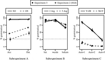
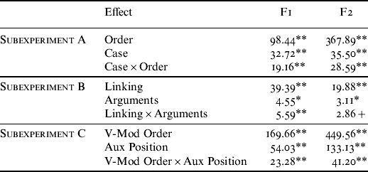
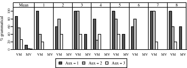
Figure 4 shows the results for Experiment 3 in terms of percentages ‘grammatical’ (filled circles). For ease of comparison, the results for the SGJ part of Experiment 2 are also shown (open circles). The reference sentence was judged as grammatical 27% of the time. For the two prior experiments, this value was 33% in Experiment 1 and 17% in Experiment 2. Table 4 summarizes all ANOVA results obtained for Experiment 3.
Percentages of ‘grammatical’ judgments in Experiment 3; the vertical lines represent standard errors by participants. The corresponding results of the SGJ part of Experiment 2 are also shown (open circles, slightly shifted to the left). The horizontal dotted lines represent the mean judgments given to the reference sentence in Experiment 3.

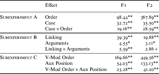
ANOVA results for Experiment 3. F1=analysis by participants; F2=analysis by items. **=p<.01; *=p<.05; +=p<.1.
7.2.1 Subexperiment A: word order and case
As in the preceding subexperiments requiring binary grammaticality judgments, the two main factors of Order and Case and the interaction between them were all highly significant. The interaction again reflects the finding that SO sentences received 96% ‘grammatical’ judgments whether containing an accusative or a dative object. With OS order, in contrast, sentences with a dative object received significantly more ‘grammatical’ judgments than sentences with an accusative object (47% vs. 26%).
7.2.2 Subexperiment B: argument alternations
The two main factors were significant. The interaction between them was fully significant in the participant analysis but just failed significance in the item analysis (p=.062). Overall, active sentences and regular-passive sentences did not differ from each other (92% for both) whereas recipient-passive sentences were judged significantly worse (72%). In addition, three-argument sentences were judged slightly better than two-argument sentences when sentences were in the active voice (94% vs. 90%) or when sentences exhibited the recipient passive (77% vs. 67%); regular-passive sentences, in contrast, were judged slightly worse when containing three instead of two arguments (90% vs. 94%). As in the SGJ subexperiments, the difference was significant only for the recipient passive.
7.2.3 Subexperiment C: verb-cluster linearization
As in all prior subexperiments, the two main effects as well the interaction between them were highly significant. When the main verb preceded the modal verb (‘V<Mod’), all three auxiliary positions differed significantly from each other (‘Aux=1’ vs. ‘Aux=2’ vs. ‘Aux=3’: 84% vs. 58% vs. 22%). When the modal verb preceded the main verb (‘V<Mod’), only a one-way distinction turned up (‘Aux=1’: 15% vs. ‘Aux=2’ and ‘Aux=3’: 3% and 2%).
7.3 Discussion
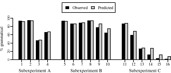
For most conditions, the results of Experiment 3 show a striking resemblance to the results of the two preceding experiments. This is most easily seen in figure 4, where the results of the current experiment and the SGJ results of Experiment 2 are plotted on a single graph for each subexperiment. Figure 4 has sixteen means: 4 (A)+6 (B)+6 (C). Fourteen out of these sixteen means differ by less than 6%. The only two conditions which differ more substantially, namely by about 20%, are the two OS conditions of Subexperiment A. We will discuss this particular discrepancy in the general discussion.
To quantify the correspondence between the three experimental methods used in this and the preceding experiments, we computed the correlations between the results of the current experiment with the ME results of Experiment 1 and with the SGJ results of Experiment 2 (that is, with the first part of each experiment). We also repeat the correlations between the ME results of Experiment 1 and the SGJ results of Experiment 2 for easy comparison. (16) shows the correlations for sentence means and for grand means. Correlations across participants are not possible because the experiments involved different participants.
(16)
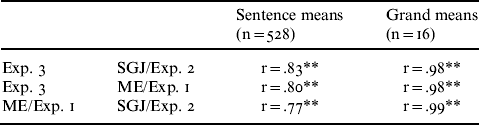
The table in (16) shows strong correlations between the results of the current experiment and the ME and SGJ results of the preceding experiments. These correlations are as high as those found between the results of the preceding experiments. Note finally that the overall percentages of sentences judged as grammatical are also quite close across all three experiments: 61.3% in Experiment 1, 65.5% in Experiment 2, and 63.4% in the current experiment.
In summary, with the exception of the two types of OS sentences included in Subexperiment A, the offline results obtained in Experiment 3 are very similar to the online results obtained in the SGJ subexperiment of Experiment 2. When the two OS conditions of Subexperiment A are excluded, the mean of the absolute differences between offline and online judgments for the remaining fourteen syntactic conditions is just 2.09%. This close correspondence came as a surprise even for us. We had expected that binary grammaticality judgments obtained under offline conditions – conditions closely matching those of traditional grammaticality judgments – would show a trend toward the extremes, either toward full grammaticality (approaching 100%) or toward full ungrammaticality (approaching 0%). Furthermore, we expected that prescriptive grammar would have a strong effect on offline grammaticality judgments. However, neither expectation was borne out by the results of Experiment 3. Take Subexperiment C on verb-cluster formation as an example. Of the six possible permutations for a cluster with three verbs, only one is grammatical according to the grammar of Standard German (the order 1–3–2 with complete auxiliary inversion). This simple, prescriptive two-way distinction notwithstanding, the results of Experiment 3 show several gradiations between fully grammatical and fully ungrammatical structures. Thus, contrary to what we had expected, averaged binary grammmaticality judgments can reveal fine distinctions whether obtained under timed conditions or not.
8. Modeling grammaticality judgments
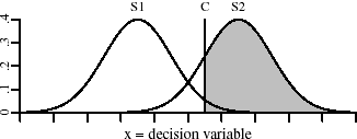
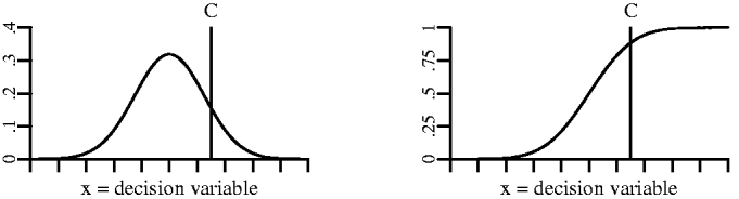
In this section, we propose a model of grammaticality judgments based on SignalDetectionTheory (SDT). This model gives a high-level characterization of the mental processes that are responsible for converting a gradient percept of sentence acceptability into an overt binary grammaticality judgment.
SDT is a general theory of how stimuli are classified into discrete categories (cf. Green & Swets Reference Green and Swets1966, MacMillan & Greelman Reference MacMillan and Greelman1991). In the simplest case, stimuli that vary along a single dimension have to be sorted into two response categories. In one situation, a stimulus is only presented some of the time (normally against some background noise), and the two response categories are ‘Yes, there was a stimulus’ and ‘No, there was no stimulus’; this procedure gave the theory its name. In another situation, a stimulus is always presented and participants have to decide to which of two stimulus classes the stimulus belongs. For example, participants in an experiment might be shown a list of words in an initial study phase. In the following experimental phase, they are then shown a second list in which words seen in the first phase are intermingled with words not seen before. The task is to classify each word according to whether it has been seen before or not.
According to SDT, a decision in an experiment like this comes about as follows. First, when participants see a word during the experimental phase, they register how familiar the word appears to them. Words which have been encountered during the study phase will on average have a higher familiarity value than words which have not been seen before. The familiarity values that are registered for the two stimuli classes are assumed to exhibit some normally distributed variability around the respective means, as illustrated in figure 5.
The normal distribution associated with two different stimuli S1 and S2. The decision variable is plotted on the x-axis; probability is plotted on the y-axis. The vertical line labeled ‘c’ represents the decision criterion.
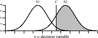
Figure 5 shows the normal distribution associated with two stimuli classes S1 and S2. The x-axis represents the decision variable, which in our example experiment would be the perceived familiarity of the word presented for classification. On average, stimuli from class S1 (=words not seen before) will receive a lower familiarity value than stimuli from class S2 (=words seen before). In order to decide whether a given stimulus belongs to class S1 or class S2, a participant follows a so-called decision criterion. In figure 5, the decision criterion is represented by the vertical line labeled ‘c’. When the familiarity value registered for a stimulus is below the decision criterion, the participant answers ‘not seen before’; when it is above the decision criterion, the answer is ‘seen before’. Note that when the two distributions overlap to a non-negligible degree, as they do in figure 5, it is impossible to select a decision criterion leading to errorless performance. In our example experiment, some new words will be erroneously classified as ‘seen before’ (the part of distribution S1 to the right of the decision criterion) and some old words will be classified as ‘not seen before’ (the part of distribution S2 to the left of the decision criterion).
Since the task of judging a sentence as either grammatical or ungrammatical has the same structure as the simple recognition experiment described above, SDT lends itself to an analysis of grammaticality judgments. In order to apply the theory, we decompose the process of giving a binary grammaticality judgment into two major steps. During the first step, each sentence is assigned a continuous acceptability value. The second step maps this continuous value onto a binary classification, which in turn determines the overt response. We thus arrive at the abstract model of grammaticality judgments shown in (17).
(17)

The first step in the model in (17) encompasses all mental processes that lead from the perceptual analysis of an input sentence to the computation of a continuous acceptability value. In accordance with related work in this area (e.g. Schütze Reference Schütze1996), we assume that every sentence is analyzed by the language comprehension mechanisms as fully as possible, independent of its ultimate acceptability. Although this is clearly not the primary purpose of language comprehension, the comprehension processes thereby deliver an acceptability score as an automatic side effect. Specifying this step in more detail would presuppose a working model of the human parsing device and a syntactic theory capable of determining graded acceptability values, either on its own or in collaboration with the parsing device. In both regards, a number of promising theories exist, but singling out any of them as most appropriate for our current purposes is beyond the scope of the present paper.
The second step of the model in (17) maps the continuous acceptability values obtained during the initial step onto binary grammaticality judgments. This step works in the same way as described above for the example experiment used to introduce SDT. Participants follow a decision criterion and classify every sentence with an acceptability score below the decision criterion as ungrammatical and every sentence with an acceptability score above the decision criterion as grammatical.
How well does our simple model of binary grammaticality judgments fare against the experimental results presented above? In order to answer this question, we fitted the model to the experimental data on several levels of generality. First, we fitted the model on the level of individual judgments, separately for Experiment 1 and Experiment 2. The only parameter to estimate was the criterion value c. We estimated c on the basis of the overall proportions of ‘grammatical’ judgments. In both experiments, 2280 individual judgments were given. In Experiment 1, the response ‘grammatical’ made up 61.3% of these judgments. An estimated criterion value of zero resulted in the closest mean value of predicted ‘grammatical’ judgments, namely 61.8%. For Experiment 2, the criterion value giving the closest fit on this level was also zero; here, an observed percentage of ‘grammatical’ judgments of 65.4% is matched by a predicted percentage of ‘grammatical’ judgments of 64.2%.
Insofar as the proposed model is correct, estimating the criterion value in the global way just described should also correctly predict the judgments in each of the 16 syntactic conditions of our three subexperiments. In order to assess the validity of this prediction, we computed the R2 values holding between the 16 means for the observed judgments and the 16 mean values for the predicted judgments. For Experiment 1, we got a very high R2 value of .97 and for Experiment 2 a high but somewhat lower value of .88. The fit between model and data is thus quite good. This is especially noteworthy given that just a single parameter was estimated. However, as with all intra-experimental comparisons, these fits must be complemented by a cross-experimental fit. As before, we use the ME results from Experiment 1 and the SGJ results from Experiment 2 for this purpose. Because different speakers took part in the two experiments, we can no longer evaluate the model on the level of individual judgments but have to rely on sentence means instead.
In doing so, we make use of the fact that any probability density function has an associated probability distribution function. This is illustrated in figure 6. The left-hand side of figure 6 is a normal probability density function as already shown in figure 5. Such a function is defined by two parameters, the mean  and the standard deviation. We assume that every sentence is associated with its own density function. The mean of this function is equated with the mean acceptability score that the sentence received in the ME part of Experiment 1. The standard deviation is assumed to be identical for all sentences and is a free parameter of the model. The area under the function to the left of c gives the proportion of ‘ungrammatical’ judgments; the area to the right of c is the proportion of ‘grammatical’ judgments.
Probability density function (left-hand side) and probability distribution function (right-hand side). The vertical line labeled ‘c’ represents the decision criterion.
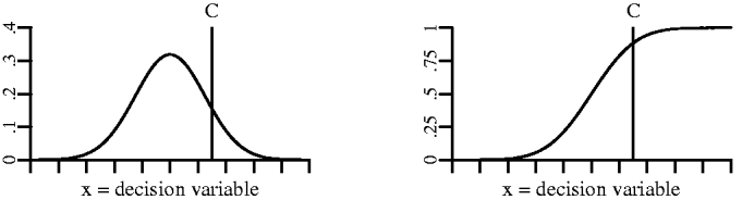
These proportions can be read off the distribution function that comes with every density function. In figure 6, the density function is shown on the left and the corresponding distribution function on the right. For every value on the x axis, the distribution function gives the summed probability of obtaining a value less than x. In our case, we set x to the value of the decision criterion c; the corresponding value of the distribution function is thus the predicted percentage of ‘ungrammatical’ judgments (because the function gives the probability of values to the left of x); percentages of ‘grammatical’ judgments are 1 minus the value of the distribution function. In this way, for every sentence the predicted percentage of ‘grammatical’ judgments can be computed from its ME acceptability score.
For the SGJ part of Experiment 2, we derived percentages of ‘grammatical’ judgments from the ME part of Experiment 1 in the way just described, with the decision criterion set to zero as before and the second free parameter, the standard deviation associated with each sentence, set to .15. Figure 7 plots the mean percentages of ‘grammatical’ judgments for our sixteen syntactic conditions; the black bars are the means observed in the SGJ part of Experiment 2; the white bars are the means predicted by our SDT model. Figure 7 reveals a very close correspondence between observed and predicted means. This is confirmed by a high R 2 value of .98.
Plot of observed means (SGJ part of Experiment 2) and means predicted by the SDT model described in the text. The sixteen conditions of the three subexperiments are numbered in accordance with the result tables in Appendix A.
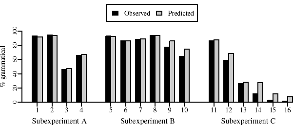
In summary, we have made use of SDT in order to formulate a model of how continuous acceptability scores are converted into binary grammaticality judgments. Despite its simplicity, the model achieved a good fit between predicted and observed data. This once more underscores the finding of a simple, rule-governed relationship between continuous acceptability ratings and binary grammaticality judgments.
So far, our model is an abstract mathematical model and not a real processing model. This is especially true for the first step, which is currently nothing more than a black-box. We have hypothesized that this black-box outputs continuous acceptability scores which can be estimated from the results of ME experiments. The question of how these acceptability scores are actually computed is far beyond the scope of the present paper. We will consider one possible factor, namely frequency of usage, in the next section.
9. Frequency and perceived well-formedness
What is the source and the nature of the continuous acceptability variable which gives rise to gradient judgments when probed with the ME methodology, and which we assume to be mapped onto binary judgments when such judgments have to be given, for example by a linguist doing syntactic research or by participants in an experiment requiring timed or untimed binary grammaticality judgments? One possibility is that degrees of acceptability reflect usage-based frequencies. While mainstream generative grammar has always denied any simple relationship between well-formedness and frequency, various usage-based theories claim that the perceived acceptability of a sentence is intimately tied to its frequency of usage (for an overview, including a discussion of the many difficulties arising in relating frequency and grammaticality, see Manning Reference Manning, Bod, Hay and Jannedy2003). Below, we relate the experimental data obtained in the preceding experiments first to lexical and then to structural frequencies. Because for most of the constructions under consideration this has not yet been done, we hope that this will provide a useful addition to the empirical base for future theoretical investigations of the relationship between grammar and usage.
9.1 Lexical frequencies
Subexperiment B on argument alternations tested 42 different verbs, each occurring in one sentence. We take the judgment data for these 42 verbs in order to determine whether judgment data and corpus frequencies correlate on the level of individual lexical items. As explained in section 3.2, whether a ditransitive verb can be put into the recipient passive depends in part on lexical-conceptual constraints which are absent when ditransitive verbs are used in the active voice or when they are put into the regular passive. When looking at lexical frequencies, we should therefore find an effect at least for verbs used in the recipient passive construction.
The relevant corpus data were obtained from the Internet with the help of the search function provided by Google. For each of the 42 verbs that were included in Subexperiment B, we determined the number of hits for three types of bigrams corresponding to the three sentence types that were investigated in our experiments. Each bigram consisted of the past participle of one of the 42 verbs and one of three auxiliaries: hat ‘has’ for the condition ‘active’, wurde ‘was’ for the condition ‘regular passive’, and bekam ‘got’ for the condition ‘recipient passive’. We obtained bigram frequencies in this way because of the so-called sparse data problem; corpus searches based on existing corpora had shown that many of the bigrams of interest do not show up in corpora of moderate size. That the frequencies of rare bigrams can be reliably estimated by doing a Google search has been shown by Keller & Lapata (Reference Keller and Lapata2003). For the 42 experimental verbs, the means and ranges of the corpus search are shown in (18). Additionally, we obtained the number of hits for the past participle form for each of the 42 verbs in order to have a rough estimate of how often each verb occurs independently of any syntactic construction.Footnote 10
(18)

Because there were no systematic differences between the results of Experiments 1 and 2, we collapsed the results of the two experiments in order to obtain more stable estimates of the judgment data for the individual verbs. We also collapsed across the factor Number of Arguments because an initial inspection of the data indicated that this factor did not have any systematic effects on the issue at hand.
The table in (19) shows correlations between judgment data and two types of corpus data: first, corpus data in the form of absolute bigram frequencies (lines (1) and (2)); second, corpus data in the form of relative bigram frequencies (bigram frequency divided by the past participle frequency of the verb). Following standard practice, all correlations were computed with logarithmic frequencies.
(19)
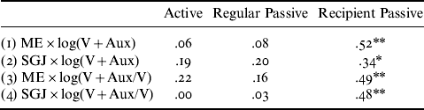
As expected at the outset, significant correlations were found for the condition ‘recipient passive’, but not for the two conditions ‘active’ and ‘regular passive’. With regard to the significant correlations for verbs in the recipient passive construction, a difference between ME and SGJ results shows up. When correlated with unconditional frequencies of verb-auxiliary bigrams, the ME results show a higher correlation than the SGJ results. When frequencies are conditioned on the overall frequency of the verb, the two judgment types yield correlations of equal size. We do not know what the reason for this difference is. In summary, the data presented in this subsection show that correlations between perceived well-formedness and corpus frequencies can be detected on the level of individual lexical items whether participants give gradient or binary judgments.
9.2 Structural frequencies
When we turn to the relationship between corpus frequency and perceived well-formedness on the structural level, a non-trivial issue arises immediately, involving the very notion of ‘structure’ itself: what do we have to count in order to determine the relationship between corpus frequency and perceived well-formedness? A general solution for this so-called grain problem does not seem to be available (see Manning Reference Manning, Bod, Hay and Jannedy2003, Crocker & Keller Reference Crocker, Keller and Fanselow2006). All results that we present below therefore have to be taken modulo the assumption that we have in fact chosen appropriate levels of granularity when comparing frequencies and judgments.
Corpus studies of word order in German (e.g. Hoberg Reference Hoberg1981, Kempen & Harbusch Reference Kempen, Harbusch, Pechmann and Habel2004, Bader & Häussler in press) have shown that the level of granularity necessary to predict whether a given sentence will occur with SO or OS order must at least include the case of the object and the animacy properties of subject and object. For present purposes, we rely on the corpus data presented in Bader & Häussler (in press) because this study provides quantitative data at the appropriate level of granularity. The sentences investigated by Bader & Häussler (in press) were randomly sampled from the newspaper corpus made available by the Institute for German Language (IDS) in Mannheim/Germany (http://www.ids-mannheim.de). The numbers shown in figure 8 are based on a set of about 700 embedded declarative complement clauses containing a subject and either an accusative or a dative object. These clauses are thus structurally identical to the ones that were investigated in Subexperiment A and the two-argument conditions of Subexperiment B.
Comparison of corpus data with experimental results (ME results of Experiment 1 and offline grammaticality judgments (OGJ) of Experiment 3). Percentage scale on left y-axis and ME scale on right y-axis. Left graph: Order of subject and object (Subexperiments A and B combined). ‘S+/O−: Acc’ is short for ‘subject[+animate] before object[−animate, accusative]’ and similarly for the other conditions. Right graph: Verb-cluster linearization (Subexperiment C).

Figure 8 shows experimental and corpus data for the order of subject and object (Subexperiments A and B) and verb-cluster linearization (Subexperiment C). Consider first the left graph in figure 8, which shows the relevant data for sentences with either SO or OS order for different combinations of animacy and case. This graph shows all conditions of Subexperiment A (both subject and object animate) as well as two conditions from Subexperiment B, namely sentences in the condition ‘active’ (SO with animate subject and inanimate accusative object) and sentences in the condition ‘regular passive’ (OS with animate dative object and inanimate subject), both pooled across the condition ‘number of arguments’; the condition ‘recipient passive’ is excluded because of its special status.
A comparison of the judgment data and the corpus data in the left-hand graph of figure 8 reveals a ceiling effect with regard to perceived well-formedness. The four most frequent sentence types were judged as highly acceptable (ME results) or grammatical (questionnaire results). In terms of corpus frequency, however, the four most frequent constructions span a range from c. 45% to c. 3%. First of all – and not unexpectedly – SO sentences with an animate subject and an inanimate accusative object occur with highest frequency. In fact, this sentence type accounts for almost half of the complete corpus. OS sentences with an inanimate subject and an animate dative object and SO sentences in which both the subject and the accusative object are animate occur with about equal frequency of somewhat more than 10%. Even less frequent are SO sentences with animate subject and animate dative object, although they still occur with some regularity. Only for the remaining sentence types – OS sentences with two animate arguments and either dative or accusative object – is a drop in perceived well-formedness found, with accusative OS sentences being judged worse than dative OS sentences. This goes along with extremely low frequencies, which appear to be identical in figure 8. In fact, however, dative OS sentences with two animate arguments occur about five times more often than corresponding accusative OS sentences, thus matching the relative ranking of the two sentence types in terms of perceived well-formedness.
Note finally that the ceiling effect visible in the left graph of figure 8 holds for the ME results and the questionnaire results alike. Ceiling effects might be a measurement artifact when binary judgments are required because percentages of ‘grammatical’ judgments cannot exceed 100%. It is therefore possible that frequency differences in the upper part of the frequency spectrum go unnoticed when grammaticality is measured by binary judgments. The measurement scale of the ME method, in contrast, is open-ended at the top and at the bottom, a fact often cited as a major advantage of this method (see Sprouse Reference Sprouse2007 for an alternative view). However, we see a ceiling effect even when looking at the ME data. The finding that a broad spectrum of frequency is mapped onto a single value of perceived well-formedness therefore cannot easily be dismissed for methodological reasons. Instead, above a certain level, no further improvement in perceived well-formedness seem to be possible.
Consider next the right graph of figure 8, which shows judgment and corpus data for Subexperiment C on verb-cluster formation. Here, we present unpublished data that we obtained from an analysis of complementizer-initial embedded clauses in the deWaC corpus, a huge tagged corpus compiled by crawling the web (described in Baroni, Bernardini, Ferraresi & Zanchetta 2009; see http://wacky.sslmit.unibo.it for further information). Based on the part-of-speech tags, we extracted all clause-final three-verb clusters consisting of a finite perfective auxiliary, a modal verb and a main verb. The numbers shown in figure 8 give the percentages of how often each of the six possible permutations of the three verbs was found.
For verb-cluster linearization, comparing corpus data and experimental results reveals a floor effect on the frequency side. Of the six possible orders, the Standard German order 1–3–2 with the main verb preceding the modal verb and the auxiliary in first position occurs with overwhelming frequency. Of the remaining five orders, the order 3–1–2 with the main verb still preceding the modal verb but the auxiliary only partially inverted to the second position still occurs with a small but non-negligible frequency. For the remaining four orders, in contrast, frequency is either zero or near zero. Nevertheless, we find systematic judgment differences among those remaining orders. In particular, the nested order 3–2–1 (V<Mod and Aux=3) and the completely inverted order 1–2–3 (Mod<V and Aux=1) were always judged better than the two orders in which the order of main and modal verb violates the Standard German order and the auxiliary follows the modal verb (orders 2–1–3 and 2–3–1). This adds to the existing evidence (e.g. Featherston Reference Featherston, Reis and Kepser2005b, Kempen & Harbusch Reference Kempen, Harbusch, Reis and Kepser2005) that native speakers are able to differentiate between syntactic structures which do either not occur at all in language use or which are exceedingly rare.
9.3 Summary: acceptability and frequency
For the syntactic constructions considered in this paper, the relationship between perceived well-formedness and frequency of occurrence does not seem to be a random one. First of all, we found effects of lexical frequency. Second, we found no instance where a syntactic structure S1 was judged as more acceptable or grammatical than a syntactic structure S2 but S2 occurred with greater corpus frequency than S1. However, not all distinctions in perceived well-formedness were reflected in the corpus counts, nor did all corpus distinctions lead to related differences in perceived well-formedness. More precisely, the pattern we found can be summarized by the two clauses in (20) (a rather similar pattern is reported in Kempen & Harbusch Reference Kempen, Harbusch and Steube2008).
- (20)
(a) Ceiling Mismatch
When perceived well-formedness is at ceiling, two syntactic structures may differ in terms of frequency despite being perceived as equally well-formed.
(b) Floor Mismatch
If frequency is at floor, two syntactic structures may differ in terms of perceived well-formedness despite both occurring with zero or near-zero frequency.
The CeilingMismatch – high values of perceived well-formedness in the face of substantial frequency differences – was attested in our data for the order of subject and object. The FloorMismatch – systematic differences in perceived well-formedness despite frequency approaching zero – was observed for word order within three-verb clusters. The finding of lexical frequency effects for recipient passive sentences but not for active or for regular passive sentences might also be due to a ceiling effect. As shown by the experimental results throughout, active and regular passive clauses were always among the structures judged best.
Let us finally note one case not covered by either of the clauses in (20). This is the case where speakers deny that they use or even know a certain structure when explicitly queried, but then use the structure nevertheless (see for example Labov Reference Labov and Austerlitz1977). Whether such cases are real exceptions must be left open because we do not know how these speakers would rate such structures in experimental settings where they have less opportunity and reason to deliberately think about the status of particular syntactic structures, in particular with regard to prescriptive norms.
10. General discussion
We have compared alternative ways of assessing the perceived well-formedness of sentences: the method of magnitude estimation, which has its origins in psycho-physics, and two methods of giving binary grammaticality judgments – speededgrammaticalityjudgments, which are an experimentally refined way of giving standard binary grammaticality judgments, and an off-line questionnaire, which comes closest to the conventional way of judging the grammaticality of sentences. In two experiments, participants had to judge sentences using both the ME and the SGJ method, either in the order ME before SGJ or the reverse. On the level of averaged mean judgments, the experiments revealed a very close correspondence between the ME results and the SGJ results. This was true whether the results were compared within or across experiments. The final experiment gathered grammaticality judgments by means of an offline questionnaire and again found results similar to those of the preceding experiments.
As a first step toward an account of the relationship between gradient and binary judgments of sentence well-formedness, we have analyzed binary grammaticality judgments as a two-step process along the lines of Signal Detection Theory. The first step consists in computing a continuous acceptability value for the given sentence. We have assumed that the values delivered by this step can be reliably estimated by the continuous ratings obtained by the ME procedure. The second step takes the gradient acceptability values computed during the first step and compares them with a preset decision criterion. All acceptability values below the decision criterion are mapped to the response ‘ungrammatical’; conversely, all acceptability values above the criterion are mapped to the response ‘grammatical’. The second step of the proposed model, thus, converts continuous acceptability values into binary grammaticality judgments. Despite its simplicity, the model resulted in a surprisingly good fit between observed and predicted data. From the success of the model we conclude that continuous acceptability ratings and binary grammaticality judgments are related to each other in a simple, rule-governed way.
In summary, the experiments presented in this paper suggest that binary grammaticality judgments are not inherently unreliable. When obtained under experimentally controlled conditions, binary grammaticality judgments can provide the same information as judgments making use of ME. Seen from a different perspective, our results can also be taken as an additional validation of the ME procedure. For someone who may be sceptical of the numerical values that participants have to assign in an ME experiment, it should be reassuring to find such a close correspondence between the results obtained with the ME procedure and those obtained when more familiar binary judgments are required. After all, what this correspondence shows is that the different experimental procedures tap the same underlying perception of well-formedness.
The high similarity between the results obtained with the ME procedure and the results obtained in experiments requiring binary judgments of grammaticality holds on the level of averaged mean values. Judgments of individual sentences by individual speakers must still be taken with caution. However, this applies both to binary judgments (or other judgments making use of a small set of discrete categories) and to gradient judgments alike. In fact, the insights gained by investigating acceptability with the help of ME were only possible because ME studies have always adhered to standard experimental practices and have relied on mean values aggregated over individual participants and sentences.
Figure 9 illustrates the problem of variability for the ME procedure and the two procedures requiring binary judgments, the SGJ procedure of Experiments 1 and 2 and the offline questionnaire of Experiment 3. This figure plots the individual mean results for each of the 30 sentences of Subexperiment C, the subexperiment concerned with the linearization of verbs in a three-verb cluster. Two conditions are shown: the Standard German order 1–3–2 is represented by filled circles, and the Colloquial German order 3–1–2 is represented by open circles. The two horizontal lines represent the mean values for these two conditions, the solid horizontal line the mean value for order 1–3–2 and the dotted horizontal line for order 3–1–2.
Mean judgment values for each of the 30 sentences of Subexperiment C on verb-cluster linearization. The upper plot shows ME results from Experiment 1; the medial plot shows SGJ results from Experiment 2; the bottom plot shows the questionnaire results from Experiment 3. See text for further details.

Figure 9 shows considerable variability at the level of individual sentences (and because these are sentence means aggregated over participants, they already abstract away from some of the observed variation). For example, the order 1–3–2 is judged better than the order 3–1–2 for the great majority of sentences, as reflected by a higher mean value for 1–3–2 than for 3–1–2. However, there are also a couple of sentences for which the relationship between 1–3–2 and 3–1–2 is reversed. This is true for all three experimental procedures represented in figure 9. Thus, relying on judgments for individual sentences would be dangerous, regardless of which method is used.
The problem of unsystematic random variation is taken care of by computing average means which abstract away from differences between speakers and sentences. The effectiveness of averaging was clearly visible in the various comparisons presented above; the highest correlations were always found on the level of grand means. However, averaging should not be considered uncritically. In essence, averaging replaces the ‘ideal speaker-hearer’ by the ‘average speaker-hearer’. An obvious question arising here is whether this average speaker-hearer corresponds to any real speaker-hearer. In the extreme, a mean value of, say, 50% for a particular syntactic structure S might be the result of averaging over two equal groups of speakers, one group always rejecting S (0%) and the other one always accepting S (100%). In this case, there would not be any real speaker who ever judges S as grammatical 50% of the time. This question is especially pressing if one subscribes to a mentalistic view of grammar according to which the individual speaker-hearer's internalized knowledge of language is the subject matter of grammatical theory (see den Dikken, Bernstein, Tortora & Zanuttini 2007 for further discussion).
Fortunately, the issue of removing systematic variation by computing average judgments is by no means an insurmountable problem.Footnote 11 As a first step in addressing this issue, we can simply take a look at each participant's individual means. For purposes of illustration, figure 10 plots the SGJ means from Subexperiment C (verb-cluster linearization) of Experiment 2 separately for the first eight speakers who participated in this experiment. Also included in this figure is a plot of the average mean values (the histogram on the left headed ‘Mean’).
Mean results (left side) and individual results for the first eight participants in Experiment 2. The results are for Subexperiment C (verb-cluster linearization) as obtained by the SGJ procedure (VM=main verb<modal verb; MV=modal verb<main verb).
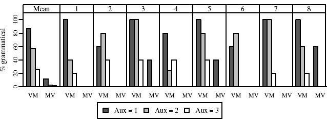
Figure 10 clearly shows variation across individual participants, although the amount of variation seems to fall within a range which might be expected given that experimental results always exhibit some amount of random variability. Tentatively, we thus conclude that the average speaker-hearer does indeed provide a reasonable representation of real speaker-hearers in the case at hand. This of course does not mean that the existing variability among real speaker-hearers always warrants the formation of an average speaker-hearer. Whether this is so must be considered anew for each experiment. That it is indeed possible to identify subgroups of speakers has been shown by Bader & Schmid (Reference Bader and Schmid2006) in an experimental study on do-support in German.
While the overall similarity between the results obtained with the different experimental procedures used in this paper is quite high, certain differences were also found. This is in particular true for the OS sentences of Subexperiment A. All experiments involving binary judgments – the SGJ subexperiments of Experiments 1 and 2 as well as the offline questionnaire of Experiment 3 – showed a substantial and statistically significant interaction between order and case: sentences with accusative object showed a clear disadvantage in comparison to sentences with a dative object when the order was OS but not when the order was SO. The ME results for Subexperiment A also showed an interaction between order and case, but it was less pronounced and not fully significant. Furthermore, the OS sentences of Subexperiment A also showed a striking difference between the SGJ results of Experiment 2 (the experiment in which the SGJ procedure was administered first) and the questionnaire results of Experiment 3 (see figure 4). Note that for the OS sentences of Subexperiment B, the regular passive sentences, a similar comparison reveals almost no differences at all.
The feature that distinguishes the OS sentences of Subexperiment A from all other syntactic conditions investigated in this paper is that OS sentences of this type are marked in terms of their information structure. Such sentences presuppose a context which imposes a narrow focus on the subject. When such sentences have to be judged without a preceding context, the judgment will depend on whether or not one can envision the necessary context. We hypothesize that people differ with regard to their willingness or ability to come up with a relevant context, and that this causes the somewhat variable results for sentences of this type. With regard to the case-by-order interaction observed in Subexperiment A, we do not know of any syntactic constraint(s) that would predict this interaction. Several competing explanations in terms of sentence processing, however, are available. In addition to linguistically motivated processing accounts in terms of case (Bader & Bayer Reference Bader and Bayer2006) or in terms of argument structures (Bornkessel & Schlesewsky Reference Bornkessel and Schlesewsky2006a), an account in terms of frequency would also be possible. Why this interaction was much stronger when binary judgments were required – either timed or untimed – than when gradient ME ratings were required is a puzzle that must be left to future research.
A final question that we would like to discuss is whether our study implies any preference for obtaining either gradient or binary judgments of sentence well-formedness. From a practical point of view, the answer is no. The first two experiments were run under tightly controlled conditions, with each participant tested individually in our laboratory, and the time needed by participants to work through the lists of experimental sentences was about the same for the ME and the SGJ method. Thus, neither method can claim an advantage in terms of the costs for running the experiment. Experiment 3 obtained binary grammaticality judgments in a less costly way because it was a questionnaire study which was completed by a large group of participants in a single session. The same, however, is also possible with magnitude estimation (e.g. Keller Reference Keller2000b).
Practical matters aside, we do not think that there are strong reasons to favor one methodology over the other. Insofar as the model presented in section 8 is correct, binary grammaticality judgments are derived from continuous acceptability values. The latter are therefore primary, and the same can be said of a method like magnitude estimation which obtains continuous judgments in a direct way. However, since traditional grammaticality judgments have received much criticism lately, we end with a short plea for them. One kind of objection that one regularly encounters when presenting SGJ experiments is that giving grammaticality judgments is felt to be an unnatural task for someone who is not a linguist. We do not think that this is true (see also Weskott & Fanselow Reference Weskott, Fanselow, Featherston and Winkler2009). At least for the population from which we recruited our participants – students of all kinds of subjects – judging the grammaticality of sentences was something almost everyone had done before. For example, when proofreading a class paper, people know that they not only have to spot typos but also grammatical errors (and even text processing software nowadays has a button for grammar checking). This does not exclude that people sometimes are unsure about whether a particular sentence is grammatically correct or not – otherwise, we wouldn't be dealing with a gradient phenomenon – but it shows that the notion of grammaticality is surely something which people are familiar with. Furthermore, if prior familiarity with the experimental task is of any relevance at all, then clearly it is the task of judging a sentence as grammatical or ungrammatical which is to be preferred. As already pointed out, many if not most of our participants had encountered this task before. Rating how much better or worse a sentence is in comparison to a given reference sentence, in contrast, is something which most participants had never done before (although, as shown by the results, they can master this task quickly and without much effort).
This brings us, finally, to a reason which in our view constitutes a real advantage of a method like SGJ over a method like ME. This concerns the interpretation of the results obtained with each method. Given the paramount role of grammaticality judgments in linguistic theorizing, knowing the mean percentage with which a given syntactic structure has been judged as grammatical appears to us to be inherently more informative than knowing the ratio by which the structure has been judged as more or less acceptable than a predefined reference sentence. For one thing, the interpretation of traditional grammaticality judgments does not depend on a reference sentence. SGJ results are thus easier to compare across experiments than ME results (for further discussion, see Featherston Reference Featherston2007). In addition, a particular percentage value is always interpretable in relation to the two boundary values of 0% and 100%. Thus, if one knows that a particular sentence type is judged as grammatical 80% of the time, one can conclude with some certainty that the sentence type is overwhelmingly accepted by native speakers, but also that there is some problem with the sentence type preventing it from approaching 100%. A similar kind of reasoning is not possible with the acceptability scores obtained by means of the ME method.
APPENDIX A
Tables of experimental results
Tables A1, A2 and A3 show all results obtained in the three experiments in numerical form. The mean acceptability scores obtained with the ME procedure and the percentages of ‘grammatical’ judgments obtained with the SGJ procedure have already been shown in graphical form in figures 1 and 2. The mean percentages of ‘grammatical’ judgments obtained in the offline questionnaire (OGJ) have been shown in figure 4. Response time (RT) data have not been shown before; they are analyzed in Appendix B. For the SGJ method, we give separate RTs for ‘grammatical’ judgments and ‘ungrammatical’ judgments; since this leads to substantial differences with regard to the number of observations that can be used for computing mean values – and thus to the reliability of the means – we also show the number of observations in each condition.
Mean acceptability scores (ME), percentages of ‘grammatical’ judgments (SGJ and OGJ), and reaction times (RTs, in ms) for Subexperiment A. For easy comparison, the results of Experiment 3 (OGJ) are shown twice.

Mean acceptability scores (ME), percentages of ‘grammatical’ judgments (SGJ and OGJ), and reaction times (RTs, in ms) for Subexperiment B. For easy comparison, the results of Experiment 3 (OGJ) are shown twice.

Mean acceptability scores (ME), percentages of ‘grammatical’ judgments (SGJ and OGJ), and reaction times (RTs, in ms) for Subexperiment C. For easy comparison, the results of Experiment 3 (OGJ) are shown twice.

Appendix B
Analysis of reaction times
Reaction times of SGJ experiments. Reaction times (RTs) in experiments using the SGJ method are only informative when they are computed separately for the two types of judgments – grammatical and ungrammatical. However, this makes it difficult or even impossible to analyze RTs by standard ANOVAs with either participants or items as random effects because of the problem of empty cells.
We therefore do not provide analyses of RTs for each individual subexperiment by means of ANOVAs, but present instead a statistical analysis of the relationship between RTs and well-formedness. This relationship is shown in figure A1. This figure is based on the ME data from Experiment 1 and the SGJ data from Experiment 2, that is, from those subparts of each experiment which were administered first and which are therefore not subject to possible repetition effects. In the left graph of figure A1, mean RTs of the SGJ part of Experiment 2 are plotted against mean acceptability scores of the ME part of Experiment 1, separately for all 16 syntactic conditions that were included in the experiments (see tables A1, A2 and A3 in Appendix A for the experimental condition to which each number in figure 1 refers); RTs for ‘grammatical’ judgments are represented by filled circles, RTs for ‘ungrammatical’ judgments by open circles. In the right graph of figure A1, mean RTs are plotted against the percentages of judgments ‘acceptable’ that were obtained in the SGJ part of Experiment 2.
Mean SGJ reaction times for judgments ‘grammatical’ (filled circles) and judgments ‘ungrammatical’ (open circles) plotted against perceived well-formedness. Numbers indicate experimental conditions. Reaction times are from Experiment 2. Left: Mean acceptability as obtained in the ME part of Experiment 1. Right: Mean grammaticality as obtained in the SGJ part of Experiment 2.

Figure A1 exhibits two striking trends. First, the time needed to judge a sentence as grammatical decreases when perceived well-formedness increases: the fastest RTs are observed for those conditions which were judged as most well-formed, and the slowest RTs for the least well-formed conditions. Exactly the opposite holds for ‘ungrammatical’ judgments. For these judgments, RTs increase with increasing acceptability scores.
In order to assess the relationship between RTs and perceived well-formedness in a quantitative way, we fitted linear regression models with either mean acceptability (ME) or mean percentages of ‘grammatical’ judgments as a numerical predictor variable, and type of response (‘grammatical’ or ‘ungrammatical’) as a binary factorial predictor variable. In this way, it is possible to fit two lines to the data, one for each of the two possible response types. As shown by the straight lines that are included within the graphs of figure A1, the fitted models do indeed give rise to two separate lines: a decreasing line for ‘grammatical’ judgments, and an increasing one for ‘ungrammatical’ judgments. The quality of the fit is quite good both for acceptability scores (ME) (R 2=.91, p<.001) and for percentages ‘grammatical’ (SGJ) (R 2=.87, p<.001).
The strong correlation between RTs and perceived well-formedness is clearly something in need of explanation. In particular, it must be determined whether the simple SDT-based model that we have proposed in this paper can be extended to account for the RT data in addition to the judgment data, or whether a more complex model is necessary to account for both reaction times and judgment data (e.g. a diffusion model along the lines of Ratcliff Reference Ratcliff1978).
Reaction times of ME experiments The instructions of our ME experiments encouraged participants to spend no more than 10 seconds on each sentence, but there was no response deadline as in the SGJ experiments. The resulting RTs, which are shown in tables A1, A2 and A3, do not give rise to problems of empty cells. However, they include not only the time for arriving at a judgment but also the time to read and comprehend the sentences (which is the reason why they are much longer than the corresponding RTs obtained by the SGJ procedure). They therefore reflect all differences among experimental conditions resulting from lexical differences between sentences, including different amounts of lexical material. This is most clearly visible for Subexperiment B. In this subexperiment, all sentences with three arguments had substantially longer RTs in the ME results than sentences with only two arguments.
The one subexperiment in which all sentences contained exactly the same lexical material is Subexperiment C. Here, sentences differed only with respect to the order of the three elements in the verb cluster. For Subexperiment C of Experiment 1, RTs are plotted against acceptability scores in figure A2. This figure reveals a systematic relationship between RTs and acceptability scores: RTs increase with increasing acceptability. Quantitatively, this resulted in an R 2 value of .90 for the straight line that was fitted to the results.
Mean ME reaction times (Mean RT) plotted against mean acceptability scores for Subexperiment C (verb-cluster linearization) of Experiment 1. Numbers indicate experimental conditions.
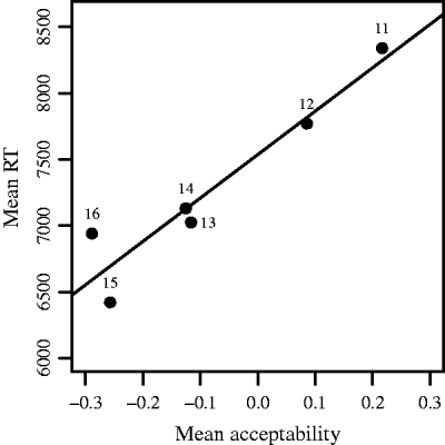
 . Because r lies between −1 and 1, its absolute value is larger than R 2.