
1. Introduction
Turbulent boundary layer trailing-edge (TE) noise (Howe Reference Howe1978) refers to the noise generated when turbulence boundary layers convect past the trailing edge of an aerofoil. It is a common aeroacoustic source in many applications involving rotating blades such as wind turbines. It has gained increasingly more attention in recent years, particularly in the wind industry. This is because the turbine blade size continues to increase, leading to increasingly large blade tip velocity. It is well known that the power of the aeroacoustic noise emission increases quickly as the blade velocity increases, and for modern wind turbines, TE noise has become the dominant noise source (Oerlemans et al. Reference Oerlemans, Fisher, Maeder and Kögler2009). As noise regulations become increasingly stringent, TE noise is also expected to become a regulatory issue for emerging commercial transport such as air taxis, small aerial vehicles and drones (Jaworski & Peake Reference Jaworski and Peake2020). Understanding TE noise and its reduction is of particular importance in these areas.
There have been numerous studies into the techniques of reducing TE noise. Some notable approaches include using porous aerofoils (Howe Reference Howe1979; Fink & Bailey Reference Fink and Bailey1980; Geyer, Sarradj & Fritzsche Reference Geyer, Sarradj and Fritzsche2009a, Reference Geyer, Sarradj and Fritzsche2010), trailing-edge brushes (Herr & Dobrzynski Reference Herr and Dobrzynski2005), surface finlets (Clark et al. Reference Clark, Daly, Devenport and Peake2016, Reference Clark, Alexander, Devenport, Glegg and Jaworski2017) and TE serrations, among which TE serrations represent a particularly effective way of reducing TE noise without severely compromising aerodynamic efficiency. The idea of using serrations was inspired by the silent flight of owls (Jaworski & Peake Reference Jaworski and Peake2020). Thorpe & Griffin (Reference Thorpe and Griffin1962) represents one of the earliest attempts to measure the aeroacoustic signature of free-flying owls. It was found that the noise generated by owls could not be detected by their experimental rig in the ultrasonic frequency range. The noise generated by owls was significantly weaker than that by other birds of similar sizes, demonstrating the owl's silent flight capability. Later experimental studies by Kroeger, Grushka & Helvey (Reference Kroeger, Grushka and Helvey1972) and Neuhaus, Bretting & Schweizer (Reference Neuhaus, Bretting and Schweizer1973) confirmed that owls did have a unique flying signature that is quieter than other birds. Consistent fly-over noise measurements by Sarradj, Fritzsche & Geyer (Reference Sarradj, Fritzsche and Geyer2011), in conjunction with fixed-wing laboratory measurement (Geyer, Sarradj & Fritzsche Reference Geyer, Sarradj and Fritzsche2009b), showed that the silent flying characteristics of owls may be related to the special features of their wings. One of these features is the wavy or serrated features around the wing's leading and trailing edge. The leading-edge serrations appear to be able to reduce the tip-vortex strength at high angles of attack, whereas TE serrations reduce the TE noise in approach/gliding flight. This inspires the technique of installing serrations on the leading and trailing edges of a wing or blade to reduce its aerodynamic noise.
Extensive research into TE noise suppression using serrations has been conducted in the past two decades. Numerous experiments show that serrations represent an effective technique to reduce TE noise. Dassen et al. (Reference Dassen, Parchen, Bruggeman and Hagg1996) conducted wind tunnel measurements to study the noise reduction effects of serrations on aerofoils and flat plates. It was shown that significant noise reductions can be achieved in both cases, for example, noise reductions up to  $8$ and
 $10$ dB were observed for aerofoils and flat plates, respectively. Maximal noise reductions were shown to occur between 1 and 6 kHz. Parchen et al. (Reference Parchen, Hoffmans, Gordner and Braun1999) undertook a similar experimental campaign, but on wind turbine blades at both full and laboratory scales. Similar noise reduction was observed, while a noise increase was reported in the high-frequency regime when serrations were misaligned with the flow direction. A decade later, Oerlemans et al. (Reference Oerlemans, Fisher, Maeder and Kögler2009) conducted field acoustic measurements on full-scale wind turbine blades using standard, optimized and serrated blades. It was shown that the optimized and serrated blades resulted in a noise reduction of
 $0.5$ and
 $3.2$ dB, respectively, for a microphone array placed on the ground. It was found that most of the noise was produced during the downwash movement of the blades. Gruber et al. (Gruber, Azarpeyvand & Joseph Reference Gruber, Azarpeyvand and Joseph2010; Gruber Reference Gruber2012) performed an extensive array of measurements to study the noise reduction effects of serrations of varying sizes. The sound power level (SWL) was obtained by integrating the noise intensity along a microphone arc placed in the mid-span plane. An average reduction of 3–5 dB was reported by using sharp sawtooth serrations. The noise reduction was found to be related to the change of convection velocity and turbulence coherence near the serrations. The serrations used by Gruber (Reference Gruber2012) were flat inserts. Chong, Joseph & Gruber (Reference Chong, Joseph and Gruber2013), however, studied non-flat serrations by directly cutting aerofoils and found similar noise reductions. However, significant boundary layer instability tones were also observed in some configurations. Recently, Leon et al. (Reference Leon, Merino-Martinez, Ragni, Avallone, Scarano, Probsting, Snellen, Simons and Madsen2016) studied the effects of serrations under deflected configurations. It was found that when the serration was aligned with the flow, a consistent noise reduction up to
 $7$ dB was obtained, whereas when the serration was misaligned, a noise increase started to appear beyond a critical Strouhal number that scaled with the boundary layer thickness and free stream velocity. The noise reduction characteristics of serrations when used specifically on flat plates were studied by Moreau & Doolan (Reference Moreau and Doolan2013) and Chong & Vathylakis (Reference Chong and Vathylakis2015). Effective noise reduction was reported in both studies. For example, a noise reduction up to
 $13$ dB was recorded by Moreau & Doolan (Reference Moreau and Doolan2013), but this was shown to be due to the attenuation of vortex shedding. Chong & Vathylakis (Reference Chong and Vathylakis2015) found that little change in the power spectral density and spanwise correlation length of the surface pressure fluctuations occurred. Instead, a pair of pressure-driven oblique vortical structures was identified by using conditional-averaging techniques. In recent years, experiments were conducted to explore the optimal serration shapes, including for example serrations with double wavelength (Chaitanya et al. Reference Chaitanya, Joseph, Narayanan and Kim2018), iron-shaped serrations (Avallone, van der Velden & Ragni Reference Avallone, van der Velden and Ragni2017), ogee serrations (Lyu, Ayton & Chaitanyan Reference Lyu, Ayton and Chaitanyan2019) etc. More details about these experiments can be found in recent studies (Lyu et al. Reference Lyu, Ayton and Chaitanyan2019).
In addition to experiments, numerical simulations are also used to study serrated TE noise. For example, Jones (Jones & Sandberg Reference Jones and Sandberg2012) performed a direct numerical simulation (DNS) of flows around a NACA0012 aerofoil with and without serrations. The serrations appeared to introduce little change into the turbulent boundary properties and an effective noise reduction was observed. Sanjosé et al. (Reference Sanjosé, Meon, Masson and Moreau2014) also performed a DNS on a serrated isolated aerofoil and reported a noise reduction of a similar magnitude. Numerical studies were also performed using the lattice Boltzmann method by Avallone et al. (Reference Avallone, van der Velden, Ragni and Casalino2018), where the link between the far-field noise and the near-field flow parameters was proposed. In addition to the noise reduction obtained by using conventional sawtooth serrations, it was shown that combed-sawtooth trailing edges can provide additional noise reduction benefits.
Both experiments and numerical simulations show that TE serration is indeed an effective method of reducing TE noise. To use serrations in practical applications, however, reliable noise prediction models are essential because they are crucial in the design of optimal serration geometries (see for example a recent study by Kholodov & Moreau Reference Kholodov and Moreau2021). Howe (Reference Howe1991a,Reference Howeb) is among the earliest researchers to model the aerodynamic noise generated by serrated trailing edges analytically. A tailored Green's function was used to formulate a noise prediction model using the blocked surface pressure statistics beneath the turbulent boundary layers. However, it has been well reported that Howe's model significantly overpredicts the noise reduction by using serrations. Later studies (Lyu, Azarpeyvand & Sinayoko Reference Lyu, Azarpeyvand and Sinayoko2015, Reference Lyu, Azarpeyvand and Sinayoko2016) showed that this is due to the Green's function being inaccurate. To improve the accuracy of the TE noise prediction, Lyu et al. (Reference Lyu, Azarpeyvand and Sinayoko2016) developed a TE noise model using Amiet's approach. Instead of using the Green's function, the Schwartszchild technique was used in conjunction with Fourier expansion in an iterative manner to enable analytical progression. The resulting prediction model yielded more realistic predictions compared to Howe's model and showed that noise reduction is achieved mainly through a destructive interference mechanism. The computation of the model involves the evaluation of nested sums, therefore needs to be optimized so as to be more suitable when used for serration optimization purposes. Recently, Ayton (Reference Ayton2018) developed a model using the Wiener–Hopf technique. The far-field sound was formulated as two infinite sums and one infinite integral, therefore consuming significant time when evaluated. However, it was shown (Lyu & Ayton Reference Lyu and Ayton2019) that the model can be further developed by evaluating the infinite integral and one of the infinite sums explicitly, and the resulting simplified model can be computed very efficiently (Lyu & Ayton Reference Lyu and Ayton2019). However, the model hinges on the semi-infinite flat plate assumption and the result is therefore strictly two dimensional. As such, the far-field pressure varies as  $1/\sqrt {r}$ instead of
 $1/r$ as
 $r\to \infty$, where
 $r$ denotes the radial distance of the observer in the plane perpendicular to the spanwise axis. When compared quantitatively with experimental data, it is unclear how far the microphone should be placed from the serration so that both the two-dimensionality and far-field assumption are valid simultaneously. More importantly, since most practical applications involve rotating blades, where three-dimensionality is crucial, a three-dimensional (3-D) accurate model would be necessary to obtain the correct prediction of TE noise for rotating blades.
A classical way to incorporate the 3-D effects is to use the two-step approach used in Amiet's model (Amiet Reference Amiet1976b), where the surface pressure due to the gust scattering by a serrated semi-infinite plate is calculated first, and the far-field sound is calculated subsequently using a surface integral assuming a finite plate. To do that, it is crucial to obtain the near-field scattered pressure on the plate surface. This poses a great difficulty as the powerful method of the steepest descent cannot be used to evaluate the inverse Fourier transform as used by Ayton (Reference Ayton2018). Considering acoustic reciprocity, this is in fact equivalent to calculating the Green's function for the acoustic scattering by serrated edges, where the acoustic source, instead of the observer, is placed in the near field. Obtaining such a Green's function would enable a TE noise model to be developed that is both three-dimensionally accurate and computationally efficient. Moreover, the Green's function itself is fundamentally important in many important aspects concerning TE noise. First, this would open the possibility of examining the consequences of many assumptions that have been open to heated debate, such as the validity of frozen turbulence that has been called into question in a number of recent studies (Ragni et al. Reference Ragni, Avallone, van der Velden and Casalino2018; Zhou et al. Reference Zhou, Liu, Zhong, Fang and Zhang2020). Second, the Green's function would provide a more intuitive understanding of the effects of serrations by showing the scattering characteristics of simple sound sources, thereby lending insights into the physical mechanism of noise reduction by using serrations, and more importantly informing on new techniques of suppressing TE noise. Last but not the least, the Green's function would permit a direct comparison between analytical scattering models and experiments. The point-source-induced sound can be readily measured in the laboratory using laser-induced monopoles. Although TE noise modelling has improved significantly, it is yet to see robust agreement between trailing-edge noise models and experiments. This is difficult, especially when realistic aerofoil geometries are considered. Often this is because the surface pressure statistics needed in the noise prediction model are rather difficult to be obtained accurately. With a controlled simple acoustic source, we can readily assess whether any deviations that exist between models and experiments are introduced by the scattering model and its underlying assumptions or by the turbulent pressure fluctuation statistics.
Although important, such an analytical Green's function remains unknown. As mentioned above, a tailored Green's function was proposed by Howe in 1991 (Howe Reference Howe1991a), but it has been shown to be problematic, especially when the serration is sharp. In this paper, we aim to develop such a Green's function analytically by using the Wiener–Hopf method. Due to mathematical symmetry, with proper transformations, it would also be applicable to the scattering by serrated leading edges (Amiet Reference Amiet1975, Reference Amiet1976b; Lyu & Azarpeyvand Reference Lyu and Azarpeyvand2017). This paper is structured as follows. Section 2 introduces the simplified model and develops the Green's function. Section 3 validates the Green's function by performing numerical integrations and finite element method (FEM) computations using COMSOL. In § 4, we show the noise directivity for a point source located near the serrated trailing edge of the flat plate due to the use of serrations and examine the effects of varying the frequency, serration amplitude, source position and Mach number. The final section concludes the paper and lists some future work.
2. Analytical derivation
To allow analytical progression, we start from a simplified model that is widely used in the literature (Howe Reference Howe1978; Lyu et al. Reference Lyu, Azarpeyvand and Sinayoko2016), i.e. the aerofoil is simplified as a flat plate placed in a uniform flow aligned in the streamwise direction, as shown in figure 1. As mentioned in § 1, the Green's function would be applicable to both trailing-edge and leading-edge scattering because of mathematical symmetry. In this paper, we use the trailing-edge scattering as an example. The flat plate is assumed to be semi-infinite, i.e. the leading edge extends to the upstream infinity and both side edges are also infinitely far away, so only the serrated trailing edge needs to be considered. We restrict our analysis to periodic serrations with a wavelength of  $\tilde {\lambda }$. The problem is non-dimensionalized using the serration wavelength
 $\tilde {\lambda }$, the speed of sound
 $\tilde {c}$ and the fluid density
 $\tilde {\rho }$. Note we have used the symbols with a tilde to denote dimensional variables, whereas those without represent non-dimensional variables. We will adhere to this convention throughout this paper unless explicitly noted otherwise. In terms of the non-dimensional variables, the serration has a wavelength
 $1$ and half-root-to-tip amplitude
 $h$, and the uniform flow from left to right has a dimensionless velocity
 $M$, which is just the Mach number.
Schematic illustration of the Green's function problem. The source represented by the black dot in the diagram is located near the edge at  $\boldsymbol {y}$ and the observer is located in the far field at
 $\boldsymbol {x}$.

A Cartesian coordinate system shown in figure 1 is used in the analysis, where  $x_1$,
 $x_2$ and
 $x_3$ denote the dimensionless streamwise, spanwise and normal-to-plate coordinates, respectively. In such a coordinate system, the profile of the serration, or the trailing edge of the plate, can be described by the periodic function
 $x_1 = hF(x_2)$, where
 $F(x_2)$ obtains a maximum value of
 $1$ and a minimum value of
 $-1$. Under the harmonic assumption of
 $\exp ({-\mathrm {i} \omega t})$, where
 $\omega$ is the non-dimensionalized angular frequency, the Green's function
 $G(\boldsymbol {x}; \boldsymbol {y},\omega )$ satisfies the following inhomogeneous convective equation (Amiet Reference Amiet1976a; Lyu et al. Reference Lyu, Azarpeyvand and Sinayoko2016):
 \begin{equation} \left(\beta^2 \frac{\partial^2 }{\partial x_1^2} + \frac{\partial^2 }{\partial x_2^2} + \frac{\partial^2 }{\partial x_3^2} + 2\mathrm{i} k M \frac{\partial }{\partial x_1} + k^2 \right) G(\boldsymbol{x}; \boldsymbol{y}, \omega) = \delta(\boldsymbol{x}-\boldsymbol{y}), \end{equation}
and the boundary condition
 \begin{equation} \left.\frac{\partial G}{\partial x_3}\right|_{x_3 ={\pm} 0} = 0, \quad x_1 < hF(x_2), \end{equation}
where  $\beta = \sqrt {1 - M^2}$ and
 $k = \omega /c$, and as shown in figure 1,
 $\boldsymbol {y}$ denotes the source position, while
 $\boldsymbol {x}$ denotes the observer position.
Note the observer location  $\boldsymbol {x}$ is often in the far field, therefore, a standard technique is to use the reciprocal theorem to calculate the adjoint Green's function
 $G^a(\,\boldsymbol {y}; \boldsymbol {x}; \omega )\equiv G(\boldsymbol {x}; \boldsymbol {y}, \omega )$ so that the advantage of a plane wave incidence can be taken. However, as we aim to include the mean-flow convection effect in this paper, i.e.
 $M \ne 0$, (2.1) is no longer self-adjoint. In other words, the adjoint Green's function
 $G^a(\,\boldsymbol {y}; \boldsymbol {x}, \omega )$ does not satisfy (2.1). Nevertheless, it can be shown that the equation where
 $G^a(\,\boldsymbol {y}; \boldsymbol {x}, \omega )$ does satisfy differs from (2.1) only by the sign in front of the term
 $2\mathrm {i} kM ({\partial }/{\partial x_1})$, i.e.
 \begin{equation} \left(\beta^2 \frac{\partial^2 }{\partial y_1^2} + \frac{\partial^2 }{\partial y_2^2} + \frac{\partial^2 }{\partial y_3^2} - 2\mathrm{i} k M \frac{\partial }{\partial y_1} + k^2 \right) G^a(\,\boldsymbol {y}; \boldsymbol{x}, \omega) = \delta(\,\boldsymbol {y}-\boldsymbol{x}). \end{equation}
Physically, this is equivalent to solving the acoustic pressure at  $\boldsymbol {y}$ while the point source is at
 $\boldsymbol {x}$, assuming a uniform flow of Mach number
 $M$ travels from right to left. In other words, the problem can be cast as ‘reciprocal’ by reversing the uniform mean flow.
Because  $\boldsymbol {x}$ is in the far field, the incidence wave from the source
 $\boldsymbol {x}$ can be approximated by a plane wave, whose amplitude depends on the distance between
 $\boldsymbol {x}$ and
 $\boldsymbol {y}$. Because of linearity, we can start with an incident wave of magnitude
 $1$, i.e.
 \begin{equation} p_{in} = \exp({-\mathrm{i} k_1 y_1 / \beta})\exp\left({\mathrm{i}\frac{kM}{\beta^2}y_1}\right) \exp({-\mathrm{i} (k_2 y_2 + k_3 y_3)}), \end{equation}
where  $k_1$ and
 $k_2$ are constants related to the radiation angle, the precise definition of which will be given later, and
 $k_3 = \sqrt {(k/\beta )^2 - k_1^2 - k_2^2}$. It can be verified that (2.4) satisfies the homogeneous version of (2.3). We decompose the total adjoint pressure field
 $G^a = p_{in} + p_r + R_s$, where the hypothetically reflected wave
 $p_r$ off an infinite flat plate is defined as
 $p_r = p_{in}(\kern0.7pt y_1, y_2, -y_3)$ and
 $R_s$ is the reflection-removed scattered pressure field. We could also have decomposed the pressure field as
 $G^a = p_{in} +G_s$, and this approach is shown in Appendix B. Note however no matter which decomposition is used, it should in no way affect the final solution.
The reflection-removed scattered wave  $R_s$ satisfies
 \begin{equation} \beta^2 \frac{\partial^2 R_s}{\partial y_1^2} + \frac{\partial^2 R_s}{\partial y_2^2} + \frac{\partial^2 R_s}{\partial y_3^2} - 2 \mathrm{i} k M \frac{\partial R_s}{\partial y_1} + k^2 R_s = 0 \end{equation}
and the following boundary conditions due to the periodicity of the serrations (Ayton Reference Ayton2018):
 $$\begin{gather} \left.\frac{\partial R_s}{\partial y_3}\right|_{y_3=0}= 0,\quad y_1 < hF(y_2); \end{gather}$$
 $$\begin{gather}\left.R_s\right|_{y_3 = 0} ={-}\exp({-\mathrm{i} k_1 y_1 / \beta}) \exp\left({\mathrm{i}\frac{kM}{\beta^2}y_1}\right)\exp({-\mathrm{i} k_2 y_2}), \quad y_1 > hF(y_2); \end{gather}$$
 $$\begin{gather}\left.R_s\right|_{y_2 = 0}= \left.R_s\right|_{y_2 = 1} \mathrm{e}^{\mathrm{i} k_2}; \end{gather}$$
 $$\begin{gather}\left.\frac{\partial R_s}{\partial y_2}\right|_{y_2 = 0} = \left.\frac{\partial R_s}{\partial y_2}\right|_{y_2 = 1} \mathrm{e}^{\mathrm{i} k_2}. \end{gather}$$
Eliminating the first-order term in (2.5) by the transformation  $R_s = \bar {R}_s \exp ({\mathrm {i} k M y_1 / \beta ^2})$, we obtain
 \begin{equation} \beta^2 \frac{\partial^2 \bar{R}_s}{\partial y_1^2} + \frac{\partial^2 \bar{R}_s}{\partial y_2^2} + \frac{\partial^2 \bar{R}_s}{\partial y_3^2} + \left(\frac{k}{\beta}\right)^2 \bar{R}_s = 0. \end{equation}
Earlier work (Ayton Reference Ayton2018) often used the non-orthogonal coordinate transformation  ${\xi _1 = (y_1 - h F(y_2)) / \beta}$,
 $\xi _2 = y_2$ and
 $\xi _3 = y_3$ to enable the use of separation of variables. We show that this coordinate transformation is not necessary and the same Wiener–Hopf equation can be obtained by using the Fourier transform directly. We follow this approach here. Introducing the stretched coordinate
 $\xi _1 = y_1 / \beta$,
 $\xi _2= y_2$,
 $\xi _3 = y_3$, we see that the governing equation reduces to
 \begin{equation} \frac{\partial^2 \bar{R}_s}{\partial \xi_1^2} + \frac{\partial^2 \bar{R}_s}{\partial \xi_2^2} + \frac{\partial^2 \bar{R}_s}{\partial \xi_3^2} + \bar{k}^2 \bar{R}_s = 0, \end{equation}
where the stretched constants are defined as  $\bar {k} = k/\beta$. Now the boundary conditions read
 $$\begin{gather} \left.\frac{\partial \bar{R}_s}{\partial \xi_3}\right|_{\xi_3=0}= 0, \quad \xi_1 < \bar{h} F(\xi_2); \end{gather}$$
 $$\begin{gather}\bar{R}_s|_{\xi_3 = 0} ={-}\exp({-\mathrm{i} (k_1 \xi_1 + k_2 \xi_2)}),\quad \xi_1 > \bar{h} F(\xi_2); \end{gather}$$
 $$\begin{gather}\bar{R}_s|_{\xi_2 = 0}= \bar{R}_s|_{\xi_2 = 1} \mathrm{e}^{\mathrm{i} k_2}; \end{gather}$$
 $$\begin{gather}\left.\frac{\partial \bar{R}_s}{\partial \xi_2}\right|_{\xi_2 = 0} = \left.\frac{\partial \bar{R}_s}{\partial \xi_2}\right|_{\xi_2 = 1}\mathrm{e}^{\mathrm{i} k_2}, \end{gather}$$
where  $\bar {h}$ is defined as
 $\bar {h} = h/\beta$. We can now perform the Fourier transform along the
 $\xi _1$ direction, i.e.
 \begin{equation} \mathcal{R}(s, \xi_2, \xi_3) = \int_{-\infty}^{\infty} \bar{R}_s(\xi_1, \xi_2, \xi_3) \exp({\mathrm{i} s \xi_1}) \,\mathrm{d} \xi_1. \end{equation}
Function  $\mathcal {R}(s, \xi _2, \xi _3)$ can be decomposed into two parts, i.e.
 \begin{align} \mathcal{R}(s, \xi_2, \xi_3) &= \int_{-\infty}^{\bar{h}F(\xi_2)}\bar{R}_s(\xi_1, \xi_2, \xi_3) \exp({\mathrm{i} s \xi_1}) \,\mathrm{d} \xi_1 \nonumber\\ &\quad + \int_{\bar{h}F(\xi_2)}^\infty \bar{R}_s(\xi_1, \xi_2, \xi_3) \exp({\mathrm{i} s \xi_1}) \,\mathrm{d} \xi_1 \nonumber\\ &= \int_{-\infty}^0\bar{R}_s(\xi_1+\bar{h}F(\xi_2), \xi_2, \xi_3) \exp({\mathrm{i} s (\xi_1+\bar{h}F(\xi_2))}) \,\mathrm{d} \xi_1 \nonumber\\ &\quad + \int_{0}^\infty \bar{R}_s(\xi_1+\bar{h}F(\xi_2), \xi_2, \xi_3) \exp({\mathrm{i} s (\xi_1+\bar{h}F(\xi_2))}) \,\mathrm{d} \xi_1\nonumber\\ &= \exp({\mathrm{i} s \bar{h} F(\xi_2)}) (\mathcal{R}^-(s, \xi_2, \xi_3) + \mathcal{R}^+(s, \xi_2, \xi_3) ) \end{align}
where functions  $\mathcal {R}^-$ and
 $\mathcal {R}^+$ are complex functions that are analytical in the lower and upper half-
 $s$ planes, respectively. A similar Fourier transform (and decomposition) is applied to the function
 $\partial \bar {R}_s / \partial \xi _3$, the result of which will be denoted by
 $\mathcal {R}^\prime$ in the rest of the paper.
Equation (2.8) then reduces to
 \begin{equation} \frac{\partial^2 \mathcal{R}}{\partial \xi_2^2} + \frac{\partial^2 \mathcal{R}}{\partial \xi_3^2} + (\bar{k}^2-s^2) \mathcal{R} = 0. \end{equation}
Equation (2.12) is the standard Helmholtz equation and its solution can be found through the usual method of separation of variables. After using the last two boundary conditions shown in (2.9), we show that (2.12) can be solved for  $\xi _3>0$ (the corresponding result for
 $\xi _3<0$ is similar due to antisymmetry) to yield
 \begin{equation} \mathcal{R}(s, \xi_2, \xi_3) = \sum_{n ={-}\infty}^{\infty} A_n(s) \exp({-\gamma_n \xi_3}) \exp({\mathrm{i} \chi_n \xi_2}), \end{equation}
where  $\chi _n = 2n{\rm \pi} - k_2$,
 $\gamma _n = \sqrt {s^2 - \kappa _n^2}$ and
 $\kappa _n = \sqrt {\bar {k}^2 - \chi _n^2}$. We see that
 $\kappa _n$ denotes the wavenumber in the
 $\xi _1-\xi _3$ plane and when
 $n=0$, it is equal to
 $\sqrt {k_1^2 + k_3^2}$. The complex function
 $A_n(s)$ will need to be determined by making use of the first two boundary conditions shown in (2.9) by using the Wiener–Hopf method, i.e.
 \begin{align} \mathcal{R}^\prime(s, \xi_2, 0) &= \exp({\mathrm{i} s \bar{h} F(\xi_2)})\sum_{n={-}\infty}^{\infty} \mathcal{R}_n^{\prime+}(s) \exp({-{\rm i} s \bar{h} F(\xi_2)}) \exp({\mathrm{i} \chi_n \xi_2}); \end{align}
 \begin{align} \mathcal{R}(s,\xi_2, 0) &= \exp({\mathrm{i} s \bar{h} F(\xi_2)}) \left(\sum_{n={-}\infty}^{\infty} \mathcal{R}_{n}^-(s) \exp({-{\rm i} s \bar{h} F(\xi_2)}) \exp({\mathrm{i} \chi_n \xi_2}) \right.\nonumber\\ &\quad \left.\vphantom{\sum_{n={-}\infty}^{\infty}} -\frac{\mathrm{i}}{s - k_1}\exp({-\mathrm{i} (k_1 \bar{h} F(\xi_2)+ k_2 \xi_2)})\right), \end{align}
where  $\mathcal {R}_n^{\prime +}(s)$ and
 $\mathcal {R}_n^-(s)$ are the expansion coefficients of functions
 $\mathcal {R}^{\prime +}(s, \xi _2, 0)$ and
 $\mathcal {R}^-(s, \xi _2, 0)$ using the basis functions
 $\exp ({-\mathrm {i} s \bar {h} F(\xi _2)}) \exp ({\mathrm {i} \chi _n \xi _2}),\ n =0, \pm 1, \pm 2 \cdots$, and they are unknown at this stage. The last exponential term in the parenthesis of (2.14b) can also be expanded and the resulting coefficients are denoted by
 $E_n(s)$. Here,
 $E_n(s)$ can be found to be
 \begin{equation} E_n(s) = \int_0^1 \exp({\mathrm{i} (s-k)\bar{h}F(\xi_2)})\exp({-\mathrm{i} 2 n {\rm \pi}\xi_2})\,\mathrm{d} \xi_2. \end{equation}
Note that  $E_n(s)$ can be arbitrary because no restriction on
 $F(\xi _2)$ has been imposed apart from it being periodic. For any arbitrary piecewise linear functions,
 $E_n(s)$ can be integrated analytically. For example, for the conventional sawtooth serration profile defined by (in one period)
 \begin{equation}
F(\xi_2)= \begin{cases} 4 \xi_2, & -\dfrac{1}{4} < \xi_2 <
\dfrac{1}{4}, \\
-4 \xi_2 + 2, & \dfrac{1}{4} <
\xi_2 < \dfrac{3}{4}, \end{cases}
\end{equation}
 $E_n(s)$ can be found as
 \begin{equation} E_n(s)= \frac{4 (s - k_1)\bar{h} \sin((s-k_1)\bar{h} - n{\rm \pi}/2)} {4 (s-k_1)^2\overline{h}^2 - n^2 {\rm \pi}^2}. \end{equation}
Upon comparing (2.13) and (2.14a) and making use of orthogonality of the basis functions  $\exp ({-\mathrm {i} s \bar {h} F(\xi _2)}) \exp ({\mathrm {i} \chi _n \xi _2}),\ n =0, \pm 1, \pm 2 \cdots$, we arrive at the following matching conditions for mode
 $n$, i.e.
 $$\begin{gather} -\gamma_n A_n(s) = \mathcal{R}^{\prime + }_n(s), \end{gather}$$
 $$\begin{gather}A_n(s) = \mathcal{R}_{n}^-(s) - \frac{\mathrm{i}}{s -k_1} E_n(s). \end{gather}$$
We can proceed by eliminating  $A(s)$ and arrive at the Wiener–Hopf equation:
 \begin{equation} \gamma_n \left(\mathcal{R}^-_n(s) - \frac{\mathrm{i}}{s-k_1} E_n(s)\right) + \mathcal{R}_n^{\prime +}(s) = 0. \end{equation}
The function  $E_n(s)$ causes much difficulty in the kernel decomposition. A recent approach (Ayton Reference Ayton2018) assumes that both
 $\mathcal {R}_n^-(s)$ and
 $\mathcal {R}_n^{\prime +}(s)$ contain the factor
 $E_n(s)$ so that a kernel factorization can proceed. However, we find that this assumption appears not to be true, in particular, this leads to results that do not strictly satisfy the boundary conditions. Moreover, as mentioned above, the results obtained by decomposing the total pressure field as either
 $G^a = p_{in} + G_s$ or
 $G^a = p_{in} + p_r + R_s$ should yield no difference to the final solution. However, it can be verified that if the assumption that
 $E_n(s)$ is a factor in
 $R_n^-(s)$ and
 $R_n^{\prime +}(s)$ is used, the two methods would yield different solutions (the two are only equal to each other for mode
 $n=0$, see Appendix D for details), which signals a potential problem with the underlying assumption. In fact, from (2.9) and (2.14a), we see that
 $E_n(s)$ represents the variation of the incident pressure on the edge. As
 $\mathcal {R}_n^-(s)$ denotes the scattered pressure upstream of the trailing edge, if
 $\mathcal {R}_n^-(s)$ had the same
 $E_n(s)$ factor as the incident wave, the scattering problem would need to be homogeneous in the spanwise direction. This can only be guaranteed if the trailing edge is a straight (or swept) edge. For serrated edges, the homogeneity condition is not satisfied and the
 $E_n(s)$ variation in
 $\mathcal {R}_n^-(s)$ cannot be guaranteed.
However, as the frequency increases, the acoustic wavelength becomes increasingly short, and the scattered pressure variation on the edge is expected to become increasingly localized and dominated by the incident phase variation; the assumption of  $E_n(s)$ dependence may be approximately valid in the high-frequency limit. Serrations are known to be more effective as the frequency increases (see for example Howe Reference Howe1991a; Gruber Reference Gruber2012; Lyu et al. Reference Lyu, Azarpeyvand and Sinayoko2016), and more importantly, it is the hydrodynamic wavelength that characterizes the incoming (gust) length scale in TE noise modelling, the localized scattering is more likely to be valid. Therefore, in the following part of this paper, we focus on this high-frequency regime aiming to develop a closed-form analytical Green's function, which can be used to develop a 3-D TE noise model.
The kernel is the standard  $\gamma _n = \sqrt {s^2 - \kappa _n^2}$, and once
 $E_n(s)$ is removed from both
 $\mathcal {R}_n^-(s)$ and
 $\mathcal {R}_n^{\prime +}(s)$, it becomes a routine procedure to be factorized as
 $\sqrt {s - \kappa _n}\sqrt {s + \kappa _n}$. Then
 $A_n(s)$ can be approximated by
 \begin{equation} A(s) ={-} \frac{1}{\gamma_n} \mathcal{R}^{\prime+}_n(s) ={-}\frac{\mathrm{i}}{\sqrt{s - \kappa_n}}\frac{\sqrt{k_1 - \kappa_n}}{s-k_1} E_n(s). \end{equation}
Substituting (2.20) into (2.13) and taking the inverse Fourier transform yields
 \begin{align} \bar{R}_s(\xi_1, \xi_2, \xi_3)) &= \sum_{n ={-}\infty}^{\infty}-\mathrm{i}(\sqrt{k_1 - \kappa_n}) \exp({\mathrm{i} \chi_n \xi_2}) \nonumber\\ &\quad \times\frac{1}{2{\rm \pi}}\int_{-\infty}^{\infty} \frac{E_n(s)}{s-k_1}\frac{1}{\sqrt{s - \kappa_n}} \exp({-\mathrm{i} s \xi_1 - \gamma_n \xi_3})\,\mathrm{d} s. \end{align}
Let  $r = \sqrt {(y_1/\beta )^2 + y_3^2}$ and
 $\cos \theta = y_1 / (\beta r)$, we have finally
 \begin{align} R_s(r,\theta, y_2) &= \frac{1}{2{\rm \pi}}\exp({\mathrm{i} k M y_1 / \beta^2}) \sum_{n ={-}\infty}^{\infty}-\mathrm{i}(\sqrt{k_1 - \kappa_n}) \exp({\mathrm{i} \chi_n y_2}) \nonumber\\ &\quad \times \left[ \int_{-\infty}^{\infty} \frac{E_n(s)}{s-k_1} \frac{1}{\sqrt{s - \kappa_n}} \exp({({-}i s \cos \theta - \gamma_n \sin\theta) r}) \,\mathrm{d} s \right], \end{align}
where  $E_n(s)$ is given by (2.15), and the integral is along the path
 $P$ shown in figure 2. Note that the integrand in (2.22) has a pole at
 $s=k_1$ and two branch points at
 $s=\pm \kappa _n$. The integral path
 $P$ has to pass above the pole at
 $s=k_1$ due to the analyticity requirement. It is, however, equivalent to integrating (2.22) along the path
 $P_0$ shown in figure 2, provided that the residue contribution from the pole is subtracted. We see from (2.17) that
 ${E_n(k_1) = \delta _{n_1}}$, therefore, it is convenient to calculate the residue, which is precisely the hypothetical reflected wave off an infinite flat plate
 $p_{r}$. Consequently, the total scattered field
 $G_s$ can be directly calculated by integrating (2.22) along the path
 $P_0$ instead, i.e.
 \begin{align} G_s(r,\theta, y_2) &= \frac{1}{2{\rm \pi}}\exp({\mathrm{i} k M y_1 / \beta^2}) \sum_{n ={-}\infty}^{\infty}-\mathrm{i}(\sqrt{k_1 - \kappa_n})\exp({\mathrm{i} \chi_n y_2}) \nonumber\\ &\quad \times \left[\int_{-\infty}^{\infty} \frac{E_n(s)}{s-k_1}\frac{1}{\sqrt{s - \kappa_n}} \exp({({-}i s \cos \theta - \gamma_n \sin\theta) r}) \,\mathrm{d} s\right], \end{align}
where the integral path in (2.23) is given by  $P_0$ as shown in figure 2.
Integral path  $P$ in (2.22), which passes around a simple pole at
 $s=k_1$ and two branch points at
 $s =\pm \kappa _n$. Note the branch point
 $\kappa _n$ can be an imaginary number depending on the value of
 $n$, which however does not affect the analyticity of the integrand along the integral path. The integral along path
 $P$ is equivalent to that along
 $P_0$ minus a residue contribution around
 $s=k_1$.

To obtain a closed-form analytical Green's function, the integral in (2.23) has to be evaluated analytically. Note that  $E_n(s)$ is arbitrary, but for all piecewise linear serration profiles,
 $E_n(s)$ can be evaluated analytically. If the far-field scattered pressure is of interest, i.e.
 $r\to \infty$, (2.23) can be quickly evaluated asymptotically by the powerful method of the steepest descent, as shown by Ayton (Reference Ayton2018). However, as we seek the Green's function, it is the near-field scattered pressure that is of our interest. The steepest descent method can no longer be used, and the contour integral in (2.23) must be integrated exactly. We show that for all piecewise linear profiles, the above complex contour integral can be integrated exactly to yield closed-form analytical solutions. We use the conventional sawtooth serration as an example in the rest of the paper, whereas the Green's functions for other common piecewise linear functions are given in Appendix C.
We begin by noting that for conventional sawtooth serrations,  $E_n(s)$ is given by (2.17), in which the sine functions can be expanded using exponential functions. To facilitate a compact notation, we define two auxiliary local polar coordinate frames, i.e.
 $(r_t, \theta _t)$ and
 $(r_r, \theta _r)$ in the stretched
 $y_1 / \beta$–
 $y_3$ plane (i.e.
 $\xi _1$–
 $\xi _3$ plane), as shown in figure 3. Here the stretch factor
 $\beta$ is to account for the background uniform flow, and when
 $M=0$, the stretched plane is just the physical
 $y_1$–
 $y_3$ plane. We see that
 $\theta _t$ and
 $\theta _r$ represent the geometric angles of the observer with respect to the tip and root of the serration in the stretched
 $y_1/\beta$–
 $y_3$ plane, respectively, while
 $r_t$ and
 $r_r$ represent their corresponding radial coordinates, respectively. With these definitions, we can obtain
 $$\begin{gather} r_t = \sqrt{r^2 + \bar{h}^2 - 2 r \bar{h} \cos\theta}, \end{gather}$$
 $$\begin{gather}\theta_t = \arccos [(r\cos\theta - \bar{h})/r_t]. \end{gather}$$
And similarly, we have
 \begin{equation} \left.\begin{gathered} r_r = \sqrt{r^2 + \bar{h}^2 + 2 r \bar{h} \cos\theta}, \\ \theta_r = \arccos [(r\cos\theta + \bar{h})/r_r]. \end{gathered}\right\} \end{equation}
Expanding the sine functions in (2.17) into exponential functions, we can show that
 \begin{align} G_s(r, \theta, y) &= \frac{1}{2{\rm \pi}}\exp({\mathrm{i} k M y_1 / \beta^2}) \sum_{n ={-}\infty}^{\infty}-\mathrm{i}(\sqrt{k_1 - \kappa_n})\exp({\mathrm{i} \chi_n y_2})\nonumber\\ &\quad \times\left( \exp\left( -\mathrm{i}\left(k_1 \bar{h}+\frac{n{\rm \pi}}{2}\right)\right) H_n(r_t, \theta_t) - \exp\left( \mathrm{i}\left(k_1\bar{h}+\frac{n{\rm \pi}}{2}\right)\right)H_n(r_r, \theta_r)\right), \end{align}
where
 \begin{align} H_n(r_i, \theta_i) = \int_{-\infty}^{\infty} \frac{-2\mathrm{i}\bar{h}}{(2(s-k_1)\bar{h})^2-(n{\rm \pi})^2} \frac{1}{\sqrt{s - \kappa_n}} \exp({({-}i s \cos \theta_i - \gamma_n \sin\theta_i)r_i}) \,\mathrm{d} s \end{align}
and  $(r_i, \theta _i)$ can take the value of either
 $(r_t, \theta _t)$ or
 $(r_r, \theta _r)$.
Definition of the two geometrical angles  $\theta _t$ and
 $\theta _r$ and their corresponding radial coordinates
 $r_t$ and
 $r_i$.

To integrate (2.27), when  $n\ne 0$, we may expand the first factor of the integrand as partial fractions, i.e.
 \begin{equation} \frac{-2\mathrm{i}\bar{h}}{(2(s-k_1)\bar{h})^2-(n{\rm \pi})^2}={-} \frac{\mathrm{i} \bar{h}}{n {\rm \pi}}\left[\frac{1}{2(s-k_1)\bar{h} - n{\rm \pi}} - \frac{1}{2(s-k_1)\bar{h} + n{\rm \pi}}\right]. \end{equation}
Equation (2.27) can then be written as the difference between two integrals, i.e.
 \begin{equation} H_n(r_i, \theta_i) ={-}\frac{\mathrm{i}}{2n{\rm \pi}}[D_n^+(r_k, \theta_i) - D_n^-(r_k, \theta_i)], \end{equation}
where
 \begin{equation} D_n^\pm(r_k, \theta_i) =\int_{-\infty}^{\infty} \frac{1}{s-(k_1 \pm n{\rm \pi}/2 \bar{h})}\frac{1}{\sqrt{s - \kappa_n}} \exp({({-}i s \cos \theta_i - \gamma_n \sin\theta_i)r_i}) \,\mathrm{d} s. \end{equation}
We see from (2.30) that the presence of the serration introduces a modulated streamwise wavenumber of  $k_1\pm n{\rm \pi} /2\bar {h}$ in the solution. Physically, this can be understood as follows. The presence of the periodic serration modulates the wavenumber of the incoming plane wave. The incoming plane wave has a spanwise wavenumber of
 $k_2$, consequently the
 $n$th mode of the scattered pressure has a spanwise wavenumber of
 $k_2 - 2 n {\rm \pi}$, where
 $n$ is an integer. Because the serration extends in both
 $y_1$ and
 $y_2$ directions, the scattered pressure along the edge varies in both
 $y_1$ and
 $y_2$ directions. Therefore, the streamwise wavenumber must be modulated simultaneously in a similar way as the spanwise wavenumber. Because the half-wavelength (one tooth) and root-to-tip amplitude of the serration are
 $1/2$ and
 $2h$, respectively, the
 $n$th-order plane wave would have corresponding modulated streamwise wavenumbers of
 $k_1+ n{\rm \pi} /2h$ and
 $k_1- n{\rm \pi} /2h$, due to the presence of the left and right teeth, respectively. Therefore, each spanwise mode (
 $n$th for example) corresponds to two equally weighted plane waves, one with a streamwise wavenumber of
 $k_1+n{\rm \pi} /2h$ and the other with
 $k_1-n{\rm \pi} /2h$. We can define two geometrical angles representing the effective incident angles in the
 $y_1/\beta - y_3$ plane for the two plane waves, i.e.
 \begin{equation} \varTheta_n^\pm{=} \arccos \frac{k_1 \pm n {\rm \pi}/2\bar{h}}{\kappa_n}, \end{equation}
where  $n$ is an integer. Clearly, for
 $n=0$, both
 $\varTheta _0^+$ and
 $\varTheta _0^-$ reduce to
 $\varTheta _0 \equiv \arccos k_1/\kappa _0$ representing the incident angle of
 $p_{in}$.
To evaluate (2.30), we deformed the integration path  $P_0$ shown in figure 2 to the curve
 $P_1+P_2+P_3$ shown in figure 4. The path
 $P_2$ is described by
 $s= -\kappa _n \cos (\theta _i + \mathrm {i} t)$, where the real number
 $t$ varies from
 $+\infty$ to
 $-\infty$. Figure 4 shows that
 $s\to \infty$ in the second quadrant as
 $t \to +\infty$, whereas as
 $s\to \infty$ in the third quadrant,
 $t \to -\infty$. It can be shown that integration along
 $P_1$ and
 $P_3$ approaches
 $0$ as
 $|s|\to \infty$. Therefore, the integral in (2.30) can be evaluated along
 $P_2$ instead provided
 $P_2$ passes the simple pole from below. Because the deformed path
 $P_2$ intersects with the real axis at
 $-\kappa _n \cos \theta _i$, such a condition is met when
 $-\kappa _n \cos \theta _i < k_1$, i.e. when
 $\theta _i > {\rm \pi}-\arccos (k_1/\kappa _n)$. When
 $0<\theta _i < {\rm \pi}- \arccos (k_1/\kappa _n)$, we can show that a residue contribution must be added. However, this pole contribution is exactly cancelled by the jump in the resulting integral and the final solution takes the same form as that for
 $\theta _i > {\rm \pi}- \arccos (k_1 /\kappa _n)$ (see Chapter 2 of Noble (Reference Noble1958) for details). Therefore, in the rest of the paper, we choose not to distinguish the two cases. By deforming the integral along
 $P_2$ and making use of the definition of (2.31), (2.30) reduces to
 \begin{equation} D_n^\pm(r_i, \theta_i)={-}\sqrt{\frac{2}{\kappa_n}} \int_{-\infty}^{\infty}\frac{\sin\dfrac{1}{2}(\theta_i + \mathrm{i} t)} {\cos(\theta_i+\mathrm{i} t) + \cos\varTheta_n^{{\pm}}} \exp({\mathrm{i} \kappa_n r_i \cosh t}) \,\mathrm{d} t.\end{equation}
Equation (2.32) can be integrated analytically to yield (see Appendix A for more details)
 \begin{equation} D_n^\pm(r_i, \theta_i) ={-}{\rm \pi}\sqrt{\frac{2}{\kappa_n}} \frac{I(\kappa_n r_i, \theta_i; \varTheta_n^\pm)}{\sin \dfrac{1}{2}\varTheta_n^\pm}, \end{equation}
where function  $I(kr, \theta ; \varTheta )$ is the classical Fresnel solution denoting the pressure field scattered by a straight trailing edge (Noble Reference Noble1958), i.e.
 \begin{align} I(kr, \theta; \varTheta) &= \frac{\exp\left({-\mathrm{i} \dfrac{\rm \pi}{4}}\right)}{\sqrt{\rm \pi}} \left[\exp({-\mathrm{i} kr \cos(\varTheta+\theta)}) F\left(\sqrt{2kr} \cos \frac{\varTheta+\theta}{2}\right) \right. \nonumber\\ &\quad \left.-\exp({-\mathrm{i} kr \cos(\varTheta-\theta)}) F\left(\sqrt{2kr} \cos\frac{\varTheta-\theta}{2}\right)\right]. \end{align}
The Fresnel integral  $F(x)$ in (2.34) is defined as
 \begin{equation} F(x) = \int_x^\infty \mathrm{e}^{\mathrm{i} u^2} \,\mathrm{d} u \end{equation}
and can be conveniently computed using the standard error function.
Deformed path  $P_1+P_2+P_3$, where
 $P_2$ is described by the
 $s = -\kappa _n \cos (\theta _i+\mathrm {i} t)$ as
 $t$ varies from
 $+\infty$ to
 $-\infty$. When
 $t=0$, the path
 $P_2$ intersects with the real axis at
 $-\kappa _n\cos \theta _i$. When
 $-\kappa _n\cos \theta _i > k_1$ as shown above, the simple pole is crossed, and a residue contribution must be included. The case when
 $\kappa _n$ is imaginary is similar.

Having obtained the analytical result of  $D_n^\pm (r_i, \theta _i)$, it follows that
 \begin{equation} H_n(r_i, \theta_i) = \frac{\mathrm{i}}{\sqrt{2\kappa_n}n} \left(\frac{I(\kappa_n r_i, \theta_i; \varTheta_n^+)}{\sin\dfrac{1}{2}\varTheta_n^+} -\frac{I(\kappa_n r_i, \theta_i; \varTheta_n^-)}{\sin\dfrac{1}{2}\varTheta_n^-}\right), \end{equation}
where, as mentioned above, the subscript  $i$ takes the value of either
 $t$ or
 $r$. Note that in (2.36),
 $H_n(r_i, \theta _i)$ decays at least as fast as
 $n^{-3 / 2}$ as
 $n\to \infty$, and because
 $n$ appears in the denominator, (2.36) works only for
 $n\ne 0$. However, if treating
 $n$ as a real variable, we may obtain the result for
 $n=0$ by taking the limit as
 $n\to 0$. To facilitate practical computations, we also derive an explicit formula for
 $H_0(r_i, \theta _i)$ from (2.27). This can be found in Appendix B.
Substituting (2.36) into (2.26), the total scattered pressure  $G_s$ can be readily evaluated. The important fact is that (2.26) is an exact evaluation of (2.23), and therefore is not only valid in the far field, but also in the near field. When
 $r\to \infty$, (2.26) would recover the far-field approximation obtained using the steepest descent method by Ayton (Reference Ayton2018). Note again that (2.36) consists of the standard Fresnel solution describing the scattered field by a straight edge. This suggests that the pressure field scattered by the sawtooth edge is equivalent to the sum of the Floquet modes scattered by two imagined semi-infinite flat plates with their straight trailing edges located at the tip and root of the serration, respectively. This appears to be somewhat consistent with a number of previous findings showing that noise generation by serrated edges is dominated by the root or tip regions (Kim, Haeri & Joseph Reference Kim, Haeri and Joseph2016; Turner & Kim Reference Turner and Kim2017; Avallone et al. Reference Avallone, van der Velden, Ragni and Casalino2018). This view, however, results from the use of the
 $E_n(s)$ assumption and is therefore not exact. Because (2.17) is used in the derivation, (2.26) is therefore only valid for sawtooth serrations; however, as mentioned earlier, we can easily obtain analytical Green's functions for any arbitrary piecewise linear serration profiles. Appendix C contains the Green's functions for other serration profiles, such as the square shapes.
When a point source is located at  $\boldsymbol {x}$, i.e.
 $(x_1, x_2, x_3)$, the incident plane wave near the serration has an amplitude of
 \begin{equation} A(\boldsymbol{x}) ={-}\frac{1}{\beta} \frac{1}{4 {\rm \pi}R} \exp({\mathrm{i} k R / \beta}) \exp\left({-\mathrm{i}\frac{kM}{\beta^2}x_1}\right), \end{equation}
where  $R = \sqrt {(x_1/\beta )^2 + x_2^2 + x_3^2}$. Furthermore, the value of
 $k_1$ and
 $k_2$ in the definition of
 $p_{in}$ can be found to be
 \begin{equation} k_1 = \frac{k}{\beta} \frac{x_1 /\beta}{R},\quad k_2 = \frac{k}{\beta} \frac{x_2}{R}. \end{equation}
By linearity, the Green's function can be readily obtained as
 \begin{equation} G(\boldsymbol{x}; \boldsymbol{y},\omega)= G^a(\,\boldsymbol {y}; \boldsymbol{x}, \omega) = A(\boldsymbol{x}) \left(p_{in} + G_s\right), \end{equation}
where  $p_{in}$ is shown in (2.4) and
 $G_s$ is given by (2.26). Equation (2.39) is the fundamental equation of this paper. It can be seen that the Green's function consists of two terms; the first term
 $A(\boldsymbol {x}) p_{in}$ represents the sound propagating directly from the source
 $\boldsymbol {y}$ to the observer
 $\boldsymbol {x}$, while the second term
 $A(\boldsymbol {x})G_s$ represents the scattered pressure off the serrated plate then propagating to the observer
 $\boldsymbol {x}$. The direct propagating sound is trivial and most importantly does not depend on the serration profiles; therefore, it is the scattered part that we are interested in.
3. Validation
We see from § 2 that to obtain the analytical Green's function, considerable algebra is involved. Therefore, it is necessary to validate the result before the Green's function is used to study the scattering characteristics. In this section, we choose to validate the Green's function using two approaches. The first is to numerically integrate (2.23) so as to ensure that the complex analytical evaluation of the integral is correct. The second approach is to make use of the FEM technique to compute the scattered pressure under the incident wave shown in (2.4) using COMSOL so as to examine to what extent the assumption regarding  $E_n(s)$ serves as a good approximation.
Figure 5 shows a comparison between the scattered pressure  $|G_s|$ obtained by the numerical integration and from (2.26). As can be seen from figure 5(a), the scattered pressures obtained using the two approaches completely collapse along the line of
 $y_2 = 0$ in the plane of the flat plate. Similarly, the scattered pressure obtained by numerical integration along the line of
 $y_1=0$ in the flat plate plane is identical to that from (2.26). Pressure values at other locations show exactly the same agreement. This excellent agreement shows that the analytical evaluation of the contour integral in the complex
 $s$ domain is indeed correct and exact.
Comparison of the scattered pressure field  $|G_s|$ on (a)
 $y_2=0$,
 $y_3=0$ and (b)
 $y_1=0$,
 $y_3 = 0$. The serration amplitude is
 $h=10$, the wavenumber is
 $k=1$, the Mach number
 $M=0$ and the observer angle
 $\varTheta _0=\frac {3}{4}{\rm \pi}$.

Although figure 5 shows that the analytical derivation from (2.23) to (2.36) is correct, it cannot show to what extent (2.39) approximates the exact solution to (2.1). This is because (2.23) is based on the assumption of  $E_n(s)$, and to examine its validity, we need to use FEM to numerically calculate the scattered pressure so that a direct comparison between the numerical and analytical Green's functions can be made. We again choose to compare the near-field
 $|G_s|$ under the incident wave shown in (2.4).
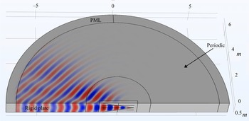
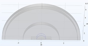
The commercial software COMSOL is used to conduct the numerical simulation, the computational domain of which is shown in figure 6. We can see that a half-cylindrical domain consisting of one serration wavelength is used. The semi-infinite plate is placed on the left-hand side of the bottom surface, as shown in figure 6. Periodic boundary conditions are used between the front and back surfaces. Perfectly matched layers (PMLs) are attached to the outer side of the domain to absorb the scattered pressure due to a plane wave incidence prescribed by (2.4). The PMLs work well for absorbing sound scattered off a finite object, but start to become less accurate to simulate a flat plate that is semi-infinitely long. To improve the accuracy of the PMLs, a small imaginary part of  $k$ (in this paper,
 $\arg {k}\approx -0.02$) is used so that the scattered pressure decays gradually as it propagates. When compared against analytical results, the same
 $k$ is used in (2.26). This is permissible and can be shown conveniently by analytical continuation. A free tetrahedral mesh is used and the resulting case has up to 4 millions degrees of freedom at the highest dimensionless frequency
 $k$. Grid independence is examined by using increasingly fine meshes that result in little change in the calculated pressure field.
Scattered pressure field  $G_s$ (only real part is shown) from FEM simulations, where
 $M=0$,
 $h=2$,
 $k=10$ and
 $\varTheta ={\rm \pi} /4$. A small imaginary part of
 $k$ is used to improve the perfectly matched layers accuracy.

The scattered near-field pressure is evaluated along two semicircles shown in blue in figure 7. The two semicircles have a dimensionless radius of  $1$ and are located in the
 $y_2=0$ and
 $y_2 =0.75$ planes, respectively. In the rest of this paper, they are referred to as the SC1 (
 $y_2=0$) and SC2 (
 $y_2 = 0.75$), respectively. In the FEM computation, the serration amplitude
 $h$, the frequency
 $k$ and the incident angle
 $\varTheta$ can all be varied. To facilitate comparison, the scattered pressure by a straight trailing edge is also computed and evaluated on the same semicircles.
Two semicircles of radius  $1$ denote the probe locations on which two scattered pressure are compared between the FEM and the analytical formula. The front semicircle is at
 $y_2=0$ while the back one is at
 ${y_2 = 0.75}$.

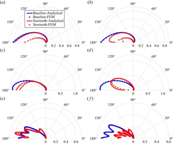
Figure 8 shows the comparison of the scattered pressure calculated by the FEM technique and the analytical Green's function at  $M=0$ and
 $\varTheta ={\rm \pi} /4$. The scattered pressure values from both the straight (blue) and serrated (red) edges at various non-dimensional frequencies are shown. Figure 8(a,b) shows the results when
 $k=2$, from which we can see that the computed pressure distribution for straight edges agrees excellently with the analytical prediction. This ensures that the PMLs work satisfactorily and the grid is sufficiently fine to resolve the pressure field. However, the computed scattered pressure for serrated edges is significantly smaller than the analytical prediction. This is expected, as the assumption about
 $E_n(s)$ dependence is not expected to be valid at this frequency. As mentioned in § 2, as the frequency increases, the scattering becomes increasingly localized and the assumption is more likely to be valid. This is indeed the case, as shown in figure 8(c,d). We can see that the baseline results continue to agree excellently with analytical predictions, but the serrated results are now in better agreement with the analytical prediction with slight deviation at large angles. In particular, figure 8(d) shows a significant change in the near-field directivity shape on SC2 due to the use of serrations, and the Green's function can capture this change well apart from the small magnitude deviation at large observer angles. As the frequency increases to
 $k=50$, figure 8(e, f) shows that the scattered pressures obtained using the two methods agree well with each other both in terms of the shape and amplitude of the directivity patterns.
Comparison of the analytical and FEM-calculated Green's function at  $M = 0$ and
 $\varTheta ={\rm \pi} / 4$ for both baseline and serrated (
 $h=1$) trailing edges on the first (SC1) and second (SC2) semicircles at various frequencies: (a)
 $k=2$, SC1; (b)
 $k=2$, SC2; (c)
 $k=10$, SC1; (d)
 $k=10$, SC2; (e)
 $k=50$, SC1; ( f)
 $k=50$, SC2.

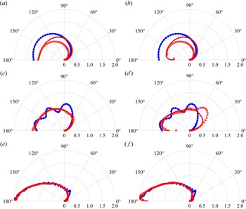
Figure 9 shows the comparison between the scattered pressure when the incident angle  $\varTheta =3/4{\rm \pi}$ for both the baseline and serrated trailing edges. When the incident angle
 ${\varTheta =3/4{\rm \pi}}$, the directivity patterns of the scattered pressure are significantly different from those at
 $\varTheta ={\rm \pi} / 4$. Nevertheless, figure 9(a,b) still clearly shows the discrepancy between the FEM and analytical results for serrated edges, while figure 9(c,d) shows that the agreement is fairly good. Again at the highest frequency
 ${k=50}$, the two lines virtually collapse, as shown in figure 9(e, f), indicating good agreement between the analytical and calculated Green's functions.
Comparison of the analytical and FEM-calculated Green's function at  $M = 0$ and
 $\varTheta =3{\rm \pi} /4$ for both baseline and serrated (
 $h=1$) trailing edges on the first (SC1) and second (SC2) semicircles at various frequencies. Legends are the same as those shown in figure 8. (a)
 $k=2$, SC1; (b)
 $k=2$, SC2; (c)
 $k=10$, SC1; (d)
 $k=10$, SC2; (e)
 $k=50$, SC1; ( f)
 $k=50$, SC2.

In summary, we see that the analytical Green's function approximates the exact Green's function reasonably well at high frequencies. A rule of thumb for the valid regime may be taken as  $kh > 10$. It is, however, worth noting that the incident plane wave is by no means limited to propagative waves. Because of analytical continuation, the Green's function must also work for evanescent waves, such as the plane-wave gusts used in TE noise modelling using Amiet's approach. In such cases, the convective Mach number of the gust is typically low and therefore it is the hydrodynamic wavenumber
 $k_1h$ that determines how localized is the scattering. Considering that this hydrodynamic wavenumber is often much larger than the acoustic wavenumber, especially for low-Mach-number applications, the
 $E_n(s)$ assumption would be more likely to hold so that (2.26) may be used to develop a 3-D TE noise prediction model. Note that although (2.26) appears complex, it can be simplified considerably when used to model TE noise because both
 $\varTheta$ and
 $\theta _i$ are equal to
 ${\rm \pi} / 2$ in the scattered surface pressure calculation. Therefore, it can be expected the resulting model can be cast into a relatively compact form that facilitates efficient evaluation.
4. Results and discussions
Having validated the analytical Green's function, we are now in a position to examine its far-field radiation characteristics and the effects of varying the frequency, serration amplitude, sound source position and Mach number using (2.39). As shown in § 2, (2.39) consists of a directly propagating incident part and a scattered part. In the rest of this section, we only examine the scattered part of Green's function, i.e.  $A(\boldsymbol {x})G_s$ shown in (2.26), because it is the scattered part
 $A(\boldsymbol {x})G_s$ that is related to the serration geometry, whereas the incident part remains unchanged no matter how the serration changes. To study the effects of the frequency, the non-dimensionalized wavenumbers
 $k=10$ and
 $k=50$ are chosen because § 3 shows that the Green's function serves as a reasonably good approximation to the exact solution at these frequencies. In the rest of this section, the far-field directivity patterns at
 $k=10$ and
 $k=50$ are shown simultaneously when the serration amplitude, source position and Mach number vary. To account for the pressure decay due to sound propagation, the scattered pressure in (2.39) is scaled by
 $4{\rm \pi} |\boldsymbol {x}|$ so that
 \begin{equation} G_{scaled} ={-}\frac{1}{\beta} \frac{|\boldsymbol{x}|}{R} \exp({\mathrm{i} k R / \beta}) \exp\left({-\mathrm{i}\frac{kM}{\beta^2}x_1}\right)G_s \end{equation}
is used to plot the directivity patterns. In the following directivity plots, the observer position is chosen to be  $|\boldsymbol {x}|=100$ away from the coordinate origin in the
 $x_2= 0$ plane. From (4.1), we see that
 $|G_{scaled}| = |G_s||\boldsymbol {x}|/\beta R$, therefore, choosing values other than
 $100$ does not change the directivity shape and magnitude in the plane
 $x_2=0$.
4.1. Effects of the serration amplitude
We first study the effects of varying the serration amplitude on the scattering characteristics. As a starting point, we let  $M=0$ so that
 $\beta =1$, i.e. the stretched coordinates are just the physical coordinates in the definition of
 $G_s$. We choose three serration lengths, i.e.
 $h=1$,
 $h=2$ and
 $h=5$, and have their scattered far-field directivity
 $|G_{scaled}|$ plotted in figure 10. The directivity plots for their corresponding straight-edge scattering are also included for reference. In all these plots, we fix the source position at
 $(\cos {\rm \pi}/4, 0.25, \sin {\rm \pi}/4)$. From figure 3, it can be seen that
 $y_2=0.25$ is the plane that passes the serration tip. For the rest of the paper, we refer to it as the tip plane, whereas
 $y_2=0.75$ is similarly referred to as the root plane. Figure 10(a,b) shows the directivity patterns for a serration amplitude of
 $h = 1$. This represents a relatively wide serration. Note we do not consider serrations wider than this, i.e. serrations with very small
 $h$ values, because that would result in very small
 $kh$ values that invalidate the
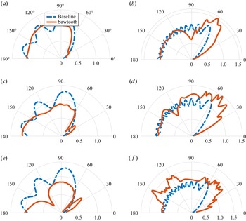
 $E_n(s)$ assumption. This however does not pose much restriction on its applications, because it is widely known that serrations with very short amplitude have little effect on reducing TE noise. We see from figure 10(a) that compared to the baseline results, the scattered pressure is slightly weaker at large observer angles, i.e.
 $\varTheta > 135^\circ$, but slightly stronger at others. As the frequency increases to
 $k=50$, we see a more pronounced radiation enhancement when
 $\varTheta < 135^\circ$ and an increasingly less obvious noise suppression at large observer angles. In addition, both the baseline and serrated directivity patterns exhibit lobes resulting from interference between the geometrically reflected and scattered pressure fields.
Far-field directivity patterns of the scattered pressure due to the baseline and serrated edges of different sizes. The source is located at  $r=1$ and
 $\theta = {\rm \pi}/4$ in the
 $y_2=0.25$ plane (passing the serration tip).(a)
 $h=1, k=10$; (b)
 $h=1, k=50$; (c)
 $h=2, k=10$; (d)
 $h=2, k=50$; (e)
 $h=5, k = 10$; ( f)
 ${h=5}, {k = 50}$.

As the amplitude of the serration increases, this tendency becomes increasingly evident, as shown in figure 10(c,d), where directivity patterns for serrations of  $h=2$ are shown. Figure 10(e, f) shows the directivity patterns when
 $h= 5$. This represents a rather long serration, and we see that the general behaviour of the scattered pressure remains similar to serrations of
 $h=2$. The difference is that the low-angle enhancement is more evident, in particular when
 $\varTheta <135^\circ$. For the long serration shown in figure 10(e, f), we see that the directivity shapes are significantly different from those of straight edges. This may be understood as follows. When the amplitude of the serration increases, the additional area of the serration extended downstream can act as an effective reflection surface for the nearby source when the observer is at low observer angles. From the directivity plots, it manifests itself as large noise radiation or even an additional lobe, as shown in figure 10(a–f). For example, because the sound source is at
 $\theta ={\rm \pi} /4$ in the tip plane in figure 10, the geometrically reflected acoustic wave would only exist in the range of
 $135^\circ < \varTheta \le 180$ for the baseline flat plate. The scattered pressure gradually decreases to
 $0$ as
 $\varTheta$ reduces to
 $0$. However, when a sufficiently large serration exists, the extended surface would provide additional reflection for a nearby source and stronger noise radiation would occur at low observer angles (e.g.
 $\varTheta < 135^\circ$) due to the additional reflection. This implies that turbulence eddies directly above the surface in the tip plane are more efficient in radiating noise to low observer angles and therefore are of more relevance for noise suppression.
The effects of serration amplitude can also be studied when the source is located at  $\theta =3{\rm \pi} /4$ in the tip plane. The results are shown in figure 11. Figure 11(a,b) shows the directivity patterns for wide serrations of
 $h=1$. Because the source is located at
 $\theta =3{\rm \pi} /4$, the scattered pressure by the baseline trailing edge has a large amplitude when
 $\varTheta > 45^\circ$ because of surface reflection. When the serrated TE is used, similar reflection exists and the resulting directivity is therefore similar to the baseline results. As the frequency increases to
 $k=50$, the behaviour remains largely similar apart from multiple lobes resulting from the interference. However, below
 $\varTheta =60^\circ$, we also see a noticeable noise increase, which again may be explained by the extended surface downstream of the source. As the serration amplitude further increases, we expect a more pronounced noise increase. This in fact can be seen in figure 11(c), where a small radiation lobe starts to appear. At
 $k=50$, the noise enhancement at
 $\varTheta <60^\circ$ is more evident. From figure 11(e), we see a roughly similar behaviour for the longest serration of
 $h=5$. However, we also note a slightly weaker radiation for
 $\varTheta >60^\circ$. This may be due to the fact that part of the flat plate upstream of the source is removed, therefore weakening a perfect reflection by a straight TE. Such weakening, however, can be expected to diminish as the frequency increases leading to increasingly localized scattering, which is indeed the case, as shown in figure 11( f). When the serration amplitude is large and the source is located in the close vicinity of the origin, it can be expected that the scattered directivity would remain roughly similar between a source at
 $\theta ={\rm \pi} /4$ and the other at
 $\theta =3{\rm \pi} /4$. By comparing figures 10( f) and 11( f), we see this is indeed the case.
Far-field directivity patterns of the scattered pressure due to the baseline and serrated edges of different sizes. The source is located at  $r=1$ and
 $\theta = 3{\rm \pi} /4$ in the
 $y_2=0.25$ plane (the serration tip plane).(a)
 $h=1$,
 $k=10$; (b)
 $h=1$,
 $k=50$; (c)
 $h=2$,
 $k=10$; (d)
 $h=2$,
 $k=50$; (e)
 $h=5$,
 $k = 10$; ( f)
 $h=5$,
 $k = 50$.

Both figures 10 and 11 show that when serrations are used, an evident noise increase occurs at some observer angles, which is particularly pronounced at high frequencies. This may seem somewhat surprising as serrations are in fact used to reduce rather than increase TE noise. This apparent contradiction arises because the Green's function developed in this paper is for a simple acoustic point source, whereas in practical applications, the sources are of a distribution type and characterized by hydrodynamic length scales that are much shorter than the acoustic wavelengths. It is known that the destructive interference introduced by serrations, which hinges on the fact that the hydrodynamic fluctuations are characterized by short length scales, plays a significant role in reducing TE noise (Howe Reference Howe1991a; Lyu et al. Reference Lyu, Azarpeyvand and Sinayoko2016; Jaworski & Peake Reference Jaworski and Peake2020). Once these hydrodynamic length scales are taken into account, significant noise reduction can be expected. Therefore, the noise directivity observed in this paper is not to be confused with that of the total TE noise.
4.2. Effects of the source position
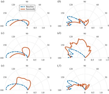
Figures 10 and 11 show the scattered pressure directivity for sound sources located in the serration tip plane. It would be interesting to understand how the scattering characteristics change when the spanwise location of the sound source changes. Figure 12 shows the directivity patterns for sound sources at  $\theta ={\rm \pi} /4$ but at different spanwise locations when
 $M=0$. Figure 12(a,b) shows the noise directivity for sources located at
 $y_2 = 0$. We see that noise is only slightly increased at low observer angles, and similarly slightly reduced at high angles. This is because the sound sources are located off the serration tip plate, therefore, the additional (weakened) reflection due to the extended (removed) surface is weaker. Significant noise increase occurs as the source moves to the tip plane, as explained in figure 10. When the spanwise location moves to
 $0.5$, we expect the resulting directivity to be identical to that in the
 $y_2 = 0$ plane due to symmetry. When the source position moves to
 $y_2 = 0.75$, i.e. in the serration root plane, the resulting directivity is shown in figure 12(e, f). It seems surprising to see an even broader lobe in the range of
 $45^\circ < \varTheta < 135^\circ$ as the source is not directly above any rigid surface. However, we note that compared to the baseline trailing edge, there do exist additional rigid surfaces downstream, albeit slightly off the plane. Furthermore, constructive interference may be expected as the two serration teeth are geometrically symmetric with respect to
 $y_2=0.75$. If this were true, we would expect a less pronounced noise increase at high frequencies, because the scattering will become localized and the scattered pressure drops more rapidly as the frequency increases. This is indeed the case, as shown in figure 12( f).
Far-field directivity patterns of the scattered pressure due to the baseline and serrated edge of  $h=2$. The source is located at
 $r=1$ and
 $\theta = {\rm \pi}/4$ in the
 $y_2=0$,
 $y_2=0.25$ and
 $y_2=0.75$ planes. (a)
 $y_2 = 0$,
 $k=10$; (b)
 $y_2 = 0$,
 $k=50$; (c)
 $y_2 = 0.25$,
 $k=10$; (d)
 $y_2 = 0.25$,
 $=50$; (e)
 $y_2=0.75$,
 $k = 50$; ( f)
 $y_2 = 0.75$,
 $k=50$.

Apart from varying the spanwise location of the source, we are also interested in the effects of varying the radial distance in the  $(y_1, y_3)$ plane, i.e.
 $\sqrt {y_1^2+y_3^2}$. As we consider the case of
 $M=0$, this distance is the same as
 $r$. For baseline TE scattering, the only characteristic length scale is the sound wavelength (apart from
 $r$). Therefore, the scattering can only depend on the non-dimensional number
 $kr$. In other words, decreasing
 $r$ would be equivalent to increasing the frequency. The use of serrated trailing edges, however, introduces two additional length scales, i.e. the wavelength and amplitude of the serration. Therefore, we expect a change in the scattering characteristics as
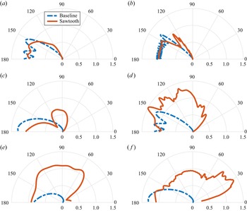
 $r$ varies. Figure 13 shows the directivity patterns for a sound source located at
 $\theta ={\rm \pi} /4$ but various
 $r$ in the tip plane. In particular, figure 13(a,b) shows the scattered directivity when the source is far from the edge at
 $r=5$. We see that the difference between the straight and serrated cases is not pronounced. This is expected because the source is relatively far away from the edge, and therefore the enhanced and weakened reflection due to the extended or removed surface would not be strong. Considerable change, however, occurs when the source moves closer to the edge to
 $r=1$, as can be seen from figure 13(c,d). At this distance, the source effectively sees parts of the reflection surface extended while others removed, and consequently the noise radiation is amplified or reduced at low or large observer angles. It is interesting to see that the baseline directivity patterns in figures 13(a) and 13(d) are identical. Indeed, without the additional length scales introduced by the serrations, the scattering would only depend on
 $kr$, which attains equal values in both cases. However, when serrations are used, we see that the directivity patterns are no longer the same even though
 $kr$ remains identical. In particular, a closer source leads to more pronounced modifications to the directivity patterns. When the source continues to move to the close vicinity of the edge, we would expect even more pronounced effects induced by the serrations. Indeed, comparing figures 13(c,d) and 13(e, f), we see that the low-angle amplification is substantial. Considering, in the serrated case, the point source is immediately above a rigid plate that does not exist in the baseline case, such strong modifications to the low-angle directivity can be expected.
Far-field directivity patterns of the scattered pressure due to the baseline and serrated edge ( $h=2$). The source is located at
 $\theta = {\rm \pi}/4$ in the
 $y_2=0.25$ plane (tip plane) and
 $r$ takes the value of
 $5$,
 $1$ and
 $0.2$.(a)
 $r=5, k=10$; (b)
 $r=5, k=50$; (c)
 $r=1, k=10$; (d)
 $r=1, k=50$; (e)
 $r=0.2, k = 10$; ( f)
 $r=0.2, k = 50$.

4.3. Effects of the Mach number
The effect of varying Mach numbers can be similarly studied. Figure 14 shows the far-field directivity patterns for a sound source located at  $(\cos (3{\rm \pi} /4), 0.25, \sin (3{\rm \pi} /4))$ but with various Mach numbers. The serration has an amplitude of
 $h=2$. Figure 14(a,b) shows the directivity at
 $M=0.2$. Compared with figure 11(c,d), we see that little change occurs at such a Mach number in both the straight and serrated cases. When we increase the Mach number to
 $M=0.5$, we start to see that the mean flow tends to increase the radiation magnitude at side angles (around
 $\varTheta =90^\circ$), whereas no amplification or reduction seems to occur at
 $\varTheta =0^\circ$ and
 $\varTheta =180^\circ$ at all. The consequence is that the directivity pattern is effectively squeezed into a thinner lobe. Such a tendency is consistent between the baseline and serrated cases, and is much more evident at the Mach number of
 $0.8$, which is shown in figure 14(e, f). For example, we see that the baseline directivity peaks at around
 $\varTheta =90^\circ$ and obtains a value of
 $1.7$, while the pressure magnitude at
 $\varTheta =180^\circ$ remains to be
 $1$.
Far-field directivity patterns of the scattered pressure due to the baseline and serrated edges at various Mach numbers. The serration has an amplitude of  $h=2$. The source is located at
 $r=1$ and
 $\theta = 3{\rm \pi} /4$ in the
 $y_2=0.25$ plane. (a)
 $M=0.2, k=10$; (b)
 $M=0.2, k=50$; (c)
 $M=0.5, k=10$; (d)
 $M=0.5, k=50$; (e)
 $M=0.8, k=10$; ( f)
 $M=0.8, k=50$.

The fact that convection amplification occurs at side angles instead of forward angles appears very strange and even contradictory to the well-known Doppler effects. It is well established that sound is amplified in the forward ( $\varTheta <{\rm \pi} /2$) arc and reduced in the backward (
 $\varTheta > {\rm \pi}/2$) arc by a factor of
 $(1-M\cos \varTheta )^{-1}$ when a point source is in motion. This would also imply that no sound amplification occurs at
 $\varTheta =90^\circ$. To understand why such a discrepancy occurs, we start with a simple where that a point source travels from left to right with a uniform Mach number
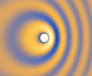
 $M$. We can choose the coordinate frame to be static relative to the medium or to the point source. The former is often used in the classical Doppler analysis while the latter in the TE noise modelling. The instantaneous pressure field generated by such a moving source can be calculated analytically and plotted in figure 15, where the Mach number is chosen to be
 $M=0.5$. Note that figure 15 is a standard result and is only included here for the following illustration purposes.
Instantaneous pressure distribution due to a moving source travelling from left to right at a Mach number of  $0.5$. The instantaneous position of the source is shown by the white circle.

In the coordinate frame that remains still to the source (e.g. with its origin fixed on the point source), the acoustic pressure at a fixed distance to the source does not possess the same phase (see figure 15). However, although not shown here in detail, it can be verified that the magnitude of the pressure is amplified by  $\beta ^{-1}$ at
 $\varTheta =90^\circ$ and remains unchanged at
 $\varTheta =0^\circ$ and
 $180^\circ$. This is precisely what we observe for our Green's function, where the TE noise source effectively remains still at the origin. In fact, the maximal value obtained at
 $\varTheta =90^\circ$ in figure 14(e) is around
 $1.7$ at
 $M=0.8$, and this is consistent with the amplification ratio of
 $\beta ^{-1}=1.67$. However, in the coordinate frame that remains still relative to the medium, we are often interested in measuring the sound at a fixed distance to its emitting position. Clearly they must have the same phase, as shown for example by the dark circles in figure 15. Figure 15 clearly shows that the emitted sound is amplified in the forward arc and reduced in the backward arc. Although not shown here in detail, it can be readily verified that the amplification ratio shown in figure 15 is precisely
 $(1-M\cos \varTheta )^{-1}$.
In summary, the seemingly strange convective behaviour shown in figure 14 is consistent with the classical Doppler effect, and the apparent contradiction is due to the use of a different coordinate frame. This shows that proper corrections have to be applied when wind tunnel results are used to predict the noise radiation directivity of practical applications.
5. Conclusion
In this paper, we develop an analytical Green's function for the acoustic scattering by serrated edges, which is in a closed form and is applicable to both TE and LE scatterings. The standard adjoint Green's function technique is used to formulate the derivation into a pressure scattering problem under a plane wave incidence. The total pressure field is then decomposed into an incident, a hypothetically reflected and a reflection-removed scattered part. The scattered field is subsequently solved using the Wiener–Hopf method. It is shown that a recent kernel factorization used in TE and LE noise modelling appears not to be uniformly valid, but may be used as a reasonable approximation in the high-frequency regime. Closed-form analytical Green's functions in the form of Fresnel integrals are obtained for any arbitrary piecewise linear serrations. Numerical integration is used to validate the derivations, which shows excellent agreement with the results given by the analytical formula. The Green's function is then compared with the scattered pressure calculated using FEM in COMSOL. The results clearly demonstrate that the  $E_n(s)$ assumption is problematic at small
 $kh$ values, but serves as reasonably good approximations at large values. The noise directivity patterns are studied as a function of the frequency, serration amplitude, source position and Mach number. It is shown that the use of serrations enhances noise radiation at low observer angles. The strength of this enhancement increases as the frequency increases. However, slight noise weakening may occur at large observer angles, but such effects diminish as the frequency increases. These directivity changes may be understood from the perspective of an extended or removed rigid reflection surface, and are therefore more evident when the source moves closer to the edge. Increasing the Mach number appears to amplify the sound at side angles but not at
 $\varTheta =0^\circ$ and
 $\varTheta =90^\circ$. This seemingly strange behaviour is the consequence of using a coordinate frame that is static relative to the TE noise source.
Due to its analytical nature, the Green's function can be evaluated quickly. Because of symmetry, it is applicable to both leading- and trailing-edge scatterings. Such a Green's function would be particularly suitable for developing a leading- or trailing-edge noise model that is both highly efficient and three-dimensionally accurate. More importantly, with a proper knowledge of the turbulence statistics inside a boundary layer, the Green's function may be used to consider the effects of non-frozen turbulence on TE noise and its reduction using serrations. These form part of our future work.
Funding
The author wishes to gratefully acknowledge the financial support from Laoshan Laboratory under the grant number of LSKJ202202000.
Declaration of interests
The author reports no conflict of interest.
Appendix A. Analytical evaluation of  $H_n^\pm (r_i, \theta _i)$ ($n\ne 0$)


To evaluate (2.32), i.e.
 \begin{equation} D_n^\pm(r_i, \theta_i)={-}\sqrt{\frac{2}{\kappa_n}} \int_{-\infty}^{\infty}\frac{\sin\dfrac{1}{2}(\theta_i + \mathrm{i} t)} {\cos(\theta_i+\mathrm{i} t) + \cos\varTheta_n^{{\pm}}} \exp({\mathrm{i} \kappa_n r_i \cosh t}) \,\mathrm{d} t, \end{equation}
we note that
 $$\begin{gather} \cos(\theta_i+\mathrm{i} t) + \cos\varTheta_n^{{\pm}} = 2 \cos \tfrac{1}{2}(\theta_i+\mathrm{i} t+\varTheta_n^\pm) \cos \tfrac{1}{2}(\theta_i+\mathrm{i} t-\varTheta_n^\pm), \end{gather}$$
 $$\begin{gather}2\sin \tfrac{1}{2}(\theta_i + \mathrm{i} t) \sin \tfrac{1}{2}\varTheta_n^\pm{=} \cos \tfrac{1}{2}(\theta_i + \mathrm{i} t -\varTheta_n^\pm) - \cos \tfrac{1}{2}(\theta_i + \mathrm{i} t +\varTheta_n^\pm). \end{gather}$$
Making use of (A2), the integrand in (A1) can be written as
 \begin{equation} \frac{1}{4 \sin \dfrac{1}{2}\varTheta_n^\pm} \left[\frac{1}{\cos \dfrac{1}{2}(\mathrm{i} t+\theta_i+\varTheta_n^\pm)} - \frac{1}{\cos \dfrac{1}{2}(\mathrm{i} t + \theta_i-\varTheta_n^\pm)}\right] \end{equation}
and consequently
 \begin{equation} D_n^\pm(r_i, \theta_i)={-}\sqrt{\frac{2}{\kappa_n}} \frac{1}{\sin \dfrac{1}{2}\varTheta_n^\pm} [N(\theta_i + \varTheta_n^\pm) - N(\theta_i - \varTheta_n^\pm)], \end{equation}
where
 \begin{equation} N(\psi) = \int_{-\infty}^{\infty}\frac{1}{4 \cos \dfrac{1}{2}(\mathrm{i} t + \psi )} \exp({\mathrm{i} \kappa_n r_i \cosh t}) \,\mathrm{d} t. \end{equation}
Equation (A5) can be evaluated by multiplying both the numerator and denominator of the integrand by  $\cos \frac {1}{2} (\mathrm {i} t - \psi )$ and making use of the odd and even properties of the integrand, resulting in
 \begin{equation} N(\psi) = \int_0^\infty\frac{\cosh \dfrac{1}{2}t \cos \dfrac{1}{2}\psi} {\cosh t + \cos\psi }\exp({\mathrm{i} \kappa_n r_i \cosh t})\,\mathrm{d} t. \end{equation}
Letting  $\tau = \sinh \frac {1}{2}t$ and
 $\cosh t = 2\tau ^2 + 1$, one can show that (Noble Reference Noble1958)
 \begin{equation} N(\psi) =\exp({-\mathrm{i} \kappa_n r_i \cos\psi})\cos \frac{1}{2}\psi\int_0^\infty \frac{\exp\left({\mathrm{i} 2\kappa_n r_i \left(\tau^2 + \cos^2 \dfrac{1}{2}\psi\right)}\right)}{\tau^2 + \cos^2 \dfrac{1}{2}\psi} \mathrm{d} \tau.\end{equation}
It is well known that
 \begin{align} &
\int_0^\infty\exp\left({\mathrm{i} 2\kappa_n r_i
\left(2\tau^2 + \cos^2
\dfrac{1}{2}\psi\right)}\right)\mathrm{d} \tau \nonumber\\
&\quad =\frac{1}{2} \exp\left({\mathrm{i} 2 \kappa_n r_i
\cos^2 \frac{1}{2}\psi}\right) \sqrt{\frac{\rm \pi}{2\kappa_n
r_i}}\exp\left({-\mathrm{i} \frac{\rm \pi}{4}}\right).
\end{align}
Integrating both side of (A8) with respect to  $r_i$, one can show that (A7) can be evaluated to
 \begin{equation} N(\psi) = \exp({-\mathrm{i}\kappa_n r_i \cos\psi})\sqrt{\rm \pi}\exp\left({-\mathrm{i} \frac{\rm \pi}{4}}\right) F\left(\sqrt{2\kappa_n r_i} \cos \frac{1}{2}\psi\right),\end{equation}
where the Fresnel integral  $F$ is defined by (2.35). Substituting (A9) into (A4), we obtain the final solution
 \begin{equation} D_n^\pm(r_i, \theta_i)={-}{\rm \pi}\sqrt{\frac{2}{\kappa_n}} \frac{I(\kappa_n r_i, \theta_i, \varTheta_n^\pm)}{\sin \dfrac{1}{2}\varTheta_n^\pm}, \end{equation}
where function  $I(\kappa _n r_i, \theta _i, \varTheta _n^\pm )$ is defined in (2.34). Using the above integral, we can quickly obtain (2.36).
Appendix B. Analytical evaluation of $H_0(r_i, \theta _i)$

When  $n=0$, (2.27) reduces to
 \begin{equation} H_0(r_i, \theta_i)={-}\frac{\mathrm{i}}{2\bar{h}} \int_{-\infty}^{\infty}\frac{1}{(s-k_1)^2}\frac{1}{\sqrt{s - \kappa_0}} \exp({({-}i s \cos \theta_i - \gamma_0 \sin\theta_i)r_i}) \,\mathrm{d} s. \end{equation}
Upon deforming onto  $P_2$, one obtains
 \begin{equation} H_0(r_i, \theta_i)={-}\frac{\mathrm{i}}{\sqrt{2\kappa_0} \kappa_0 \bar{h}} \int_{-\infty}^{\infty}\frac{\sin\dfrac{1}{2}(\theta_i + \mathrm{i} t)} {\left(\cos(\theta_i+\mathrm{i} t) + \cos\varTheta_0\right)^2} \exp({\mathrm{i} \kappa_0 r_i \cosh t}) \,\mathrm{d} t. \end{equation}
To evaluate (B2), we make use of the same trigonometric identity shown in (A2) such at
 \begin{equation} H_0(r_i, \theta_i)={-}\frac{\mathrm{i}}{\sqrt{2\kappa_0} \kappa_0 \bar{h}} \frac{1}{\sin \dfrac{1}{2}\varTheta_0} \left[M\left(\theta_i + \varTheta_0, \theta_i - \varTheta_0\right) -M\left(\theta_i - \varTheta_0, \theta_i + \varTheta_0\right)\right], \end{equation}
where
 \begin{equation} M(\psi_1, \psi_2) =\int_{-\infty}^{\infty} \frac{1}{8\cos^2 \dfrac{1}{2}(\mathrm{i} t + \psi_1)\cos \dfrac{1}{2}(\mathrm{i} t + \psi_2)} \exp({\mathrm{i} \kappa_0 r_i \cosh t}) \,\mathrm{d} t. \end{equation}
To evaluate (B4), we multiply both the numerator and denominator by  $\cos ^2 \frac {1}{2}(\mathrm {i} t - \psi _1)\cos \frac {1}{2}(\mathrm {i} t - \psi _2)$, expand using trigonometric identities, and make use of the odd and even properties of the integrand to rewrite (B4) as
 \begin{align} & \int_0^\infty\frac{(1+\cosh t \cos\psi_1)\left(\cosh \dfrac{1}{2}t + \cos \dfrac{1}{2}\psi_2 - \sinh t \sin\psi_1 \sinh \dfrac{1}{2}t \sin \dfrac{1}{2}\psi_2\right)} {(\cosh t + \cos\psi_1)^2 (\cosh t + \cos\psi_2)} \nonumber\\ &\quad \times\exp({\mathrm{i} \kappa_0 r_i \cosh t}) \,\mathrm{d} t. \end{align}
Let  $\tau =\sinh \frac {1}{2}t$ and hence
 $\cosh t = 1 + 2\tau ^2$, then (B5) reduces to
 \begin{equation} M(\psi_1, \psi_2)=\int_0^\infty \frac{\cos\left(\psi_1 + \dfrac{\psi_2}{2}\right) \tau^2 + \cos^2 \psi_1 \cos \dfrac{\psi_2}{2}} {2\left(\tau^2 + \cos^2 \dfrac{\psi_1}{2}\right)^2 \left(\tau^2 + \cos^2 \dfrac{\psi_2}{2}\right)}\exp({\mathrm{i} \kappa_0 r_i (2\tau^2 + 1)}) \,\mathrm{d} t. \end{equation}
Note that the rational expression in the integrand of (B6) can be expanded in terms of partial fractions, i.e.
 \begin{align} & \frac{\cos\left(\psi_1 + \dfrac{\psi_2}{2}\right) \tau^2 + \cos^2 \psi_1 \cos \dfrac{\psi_2}{2}}{2 \left(\tau^2 + \cos^2 \dfrac{\psi_1}{2}\right)^2 \left(\tau^2 + \cos^2 \dfrac{\psi_2}{2}\right)} \nonumber\\ &\quad =\frac{A_1}{\tau^2 + \cos^2 \dfrac{1}{2}\psi_1} +\frac{A_2}{\left(\tau^2 + \cos^2 \dfrac{1}{2}\psi_1\right)^2} + \frac{A_3}{\tau^2 + \cos^2 \dfrac{1}{2}\psi_2}, \end{align}
where
 $$\begin{gather} A_1 = \frac{-\cos \frac{1}{2}\psi_2}{2\sin^2 \dfrac{1}{2}(\psi_1 - \psi_2)}, \end{gather}$$
 $$\begin{gather}A_2 = \frac{\sin \dfrac{1}{2}\psi_1 \cos^2 \dfrac{1}{2}\psi_1}{\sin \dfrac{1}{2}(\psi_1 - \psi_2)}, \end{gather}$$
 $$\begin{gather}A_3 ={-}A_1. \end{gather}$$
The first and third partial fractions are similar to (A7), therefore can be readily evaluated. The second term can be evaluated by integrating (A8) twice with respect to  $r_i$, so that the
 $M(\psi _1, \psi _2)$ reduces to
 \begin{align}
M(\psi_1, \psi_2) &= A_1 \exp\left({-\mathrm{i}
\frac{\rm \pi}{4}}\right) \frac{\sqrt{\rm \pi}}{\cos \dfrac{1}{2}
\psi_1} \exp({-\mathrm{i} \kappa_0 r_i \cos\psi_1})
F\left(\sqrt{2\kappa_0 r_i} \cos \frac{1}{2}\psi_1\right) \nonumber\\
&\quad + A_2\exp\left({-\mathrm{i}
\frac{\rm \pi}{4}}\right) \frac{\sqrt{\rm \pi}}{\cos^3
\dfrac{1}{2} \psi_1} \exp({-\mathrm{i} \kappa_0 r_i
\cos\psi_1}) \nonumber\\
&\quad \times\left(2\mathrm{i}\kappa_0 r_i \cos^2
\frac{1}{2}\psi_1 F\left(\sqrt{2\kappa_0 r_i} \cos
\frac{1}{2}\psi_1\right) \right.\nonumber\\
&\quad \left.+\,\frac{1}{2} \sqrt{2\kappa_0 r_i \cos^2
\frac{1}{2}\psi_1} \exp\left({\mathrm{i} 2\kappa_0 r_i
\cos^2 \frac{1}{2}\psi_1}\right)
+\frac{1}{2}F\left(\sqrt{2\kappa_0 r_i} \cos
\frac{1}{2}\psi_1\right)\right) \nonumber\\
&\quad + A_3\exp\left({-\mathrm{i} \frac{\rm \pi}{4}}\right)
\frac{\sqrt{\rm \pi}}{\cos \dfrac{1}{2}
\psi_2}\exp({-\mathrm{i} \kappa_0 r_i \cos\psi_2})
F\left(\sqrt{2\kappa_0 r_i} \cos \frac{1}{2}\psi_2\right).
\end{align}
Substituting (B9) into (B3) and collecting common terms, we show that  $H_0(r_i, \theta _i)$ can be calculated explicitly as
 \begin{align} H_0(r_i, \theta_i) &= \frac{\mathrm{i}{\rm \pi}}{4\sqrt{2\kappa_0}\kappa_0 \bar{h}} \frac{1}{\sin^2\dfrac{\varTheta_0}{2}}\left[\frac{I(\kappa_0 r_i, \theta_i; \varTheta_0)}{\sin\dfrac{\varTheta_0}{2}}- \frac{(2\mathrm{i}\kappa_0 r_i) J(\kappa_0 r_i, \theta_i;\varTheta_0)}{\cos\dfrac{\varTheta_0}{2}} \vphantom{\frac{\exp\left({-\mathrm{i} \dfrac{\rm \pi}{4}}\right)}{\sqrt{\rm \pi} }}\right.\nonumber\\ &\quad \left. -\frac{\exp\left({-\mathrm{i} \dfrac{\rm \pi}{4}}\right)}{\sqrt{\rm \pi} } 2\sqrt{2\kappa_0 r_i} \sin\frac{\theta_i}{2} \exp({\mathrm{i} \kappa_0 r_i})\right], \end{align}
where the subscript  $i$ takes the value of either
 $t$ or
 $r$. The Fresnel function
 $I(\kappa _0 r_i, \theta _i; \varTheta _0)$ is defined in § 2, and
 $J(\kappa _0 r_i, \theta _i; \varTheta _0)$ is very similar to
 $I(\kappa _0 r_i, \theta _i; \varTheta _0)$, i.e.
 \begin{align}
J(\kappa_0 r_i, \theta_i; \varTheta_0) &=
\frac{1}{\sqrt{\rm \pi}} \exp\left({-\mathrm{i}
\dfrac{\rm \pi}{4}}\right)
\left[\sin(\varTheta_0+\theta_i)\exp({-\mathrm{i} \kappa_0
r_i \cos(\varTheta+\theta)})
\vphantom{\left(\sqrt{2\kappa_0 r_i} \cos
\frac{\varTheta_0-\theta_i}{2}\right)}\right.\nonumber\\
&\quad \times F\left(\sqrt{2\kappa_0 r_i} \cos
\frac{\varTheta_0+\theta_i}{2}\right)
-\sin(\varTheta_0-\theta_i) \nonumber\\
&\quad \left. \times
\exp({-\mathrm{i} \kappa_0 r_i \cos(\varTheta_0-\theta_i)})
F\left(\sqrt{2\kappa_0 r_i} \cos
\frac{\varTheta_0-\theta_i}{2}\right) \right].
\end{align}
Appendix C. Green's function for other piecewise linear serration profiles
As mentioned in § 2, the Green's function can be calculated analytically for arbitrary piecewise linear serrations. For other serration profiles, the scattered Green's function  $G_s$ can still be written as
 \begin{align} G_s(r,\theta, y_2) &= \frac{1}{2{\rm \pi}}\exp({\mathrm{i} k M y_1 / \beta^2}) \sum_{n ={-}\infty}^{\infty} -\mathrm{i}(\sqrt{k_1 - \kappa_n}) \nonumber\\ &\quad \times \left[\int_{-\infty}^{\infty}\frac{E_n(s)}{s-k_1} \frac{1}{\sqrt{s - \kappa_n}} \exp({(-{\rm i} s \cos \theta - \gamma_n \sin\theta) r}) \,\mathrm{d} s\right], \end{align}
where the integral path is given by  $P_0$, as shown in figure 2, and
 $E_n(s)$ is defined by (2.15). For square-shaped serrations,
 \begin{equation} E_n(s) = \frac{2\sin \dfrac{1}{2}n{\rm \pi}}{n{\rm \pi}}\exp\left({-\mathrm{i} \frac{1}{2}n{\rm \pi}}\right) \cos\left[(s-k_1)\bar{h} + \frac{n{\rm \pi}}{2}\right]. \end{equation}
Note that  $E_n(s)$ can be readily written as
 \begin{align} E_n(s) &= \frac{\sin \dfrac{1}{2}n{\rm \pi}}{n{\rm \pi}}\exp\left({\mathrm{i} \frac{1}{2}n{\rm \pi}}\right) \left(\exp\left({\mathrm{i} \left[(s-k_1)\bar{h} - \frac{n{\rm \pi}}{2}\right]}\right) \right.\nonumber\\ &\quad \left.+\exp\left({-\mathrm{i} \left[(s-k_1)\bar{h} - \frac{n{\rm \pi}}{2}\right]}\right)\right). \end{align}
Equation (C3) is similar to (2.17) (after trigonometric expansions), and the Green's function can be calculated in a similar manner (without performing additional integration) to yield
 \begin{align} G_s(r, \theta, y) &= \frac{1}{2{\rm \pi}} \exp({\mathrm{i} k M y_1 / \beta^2})\sum_{n ={-}\infty}^{\infty} -\mathrm{i}(\sqrt{k_1 - \kappa_n})\exp({\mathrm{i} \chi_n y_2}) \frac{\sin \dfrac{1}{2}n{\rm \pi}}{n{\rm \pi}}\exp\left({\mathrm{i} \frac{1}{2} n{\rm \pi}}\right) \nonumber\\ &\quad \times \left(\exp\left( -\mathrm{i}\left(k_1\bar{h}+\frac{n{\rm \pi}}{2}\right)\right) D_0(r_t, \theta_t) - \exp\left( \mathrm{i}\left(k_1\bar{h}+\frac{n{\rm \pi}}{2}\right)\right)D_0(r_r, \theta_r)\right), \end{align}
where  $D_0(r_i, \theta _i) \equiv D_0^+(r_i, \theta _i)\equiv D_0^-(r_i, \theta _i)$ is defined in (2.33). Note that
 $D_0(r_i, \theta _i)$ does not depend on
 $n$, which is different from that for sawtooth serrations. In fact, we can show that
 $E_n(s)$ for arbitrary piecewise linear serrations can be written in a similar form as those shown in (C3), therefore, their corresponding Green's functions can be calculated similarly in a straightforward manner. We omit a repetitive description here.
Appendix D. An alternative decomposition
When we use the decomposition  $G^a = p_{in} + G_s$ instead, the scattered wave
 $G_s(\,\boldsymbol {y};\boldsymbol {x}, \omega )$ satisfies
 \begin{equation} \beta^2 \frac{\partial^2 G_s}{\partial y_1^2} + \frac{\partial^2 G_s}{\partial y_2^2} + \frac{\partial^2 G_s}{\partial y_3^2} - 2\mathrm{i} k M \frac{\partial G_s}{\partial y_1} + k^2 G_s = 0, \end{equation}
and the following boundary conditions:
 $$\begin{gather} \left.\frac{\partial G_s}{\partial y_3}\right|_{y_3=0} = i k_3 \exp({-\mathrm{i} k_1 y_1 / \beta}) \exp\left({\mathrm{i}\frac{kM}{\beta^2}y_1}\right) \exp({-\mathrm{i} k_2 y_2}),\quad y_1 < hF(y_2); \end{gather}$$
 $$\begin{gather}G_s|_{y_3 = 0}= 0,\quad y_1 > hF(y_2); \end{gather}$$
 $$\begin{gather}G_s|_{y_2 = 0}= G_s|_{y_2 = 1} \mathrm{e}^{\mathrm{i} k_2}; \end{gather}$$
 $$\begin{gather}\left.\frac{\partial G_s}{\partial y_2}\right|_{y_2 = 0} = \left.\frac{\partial G_s}{\partial y_2}\right|_{y_2 = 1} \mathrm{e}^{\mathrm{i} k_2}. \end{gather}$$
Eliminating the first-order term in (D1) by the transformation  $G_s = \bar {G}_s \exp ({\mathrm {i} k M y_1 / \beta ^2})$, one obtains
 \begin{equation} \beta^2 \frac{\partial^2 \bar{G}_s}{\partial y_1^2} + \frac{\partial^2 \bar{G}_s}{\partial y_2^2} + \frac{\partial^2 \bar{G}_s}{\partial y_3^2} + \left(\frac{k}{\beta}\right)^2 \bar{G}_s = 0. \end{equation}
Note here, we can use either the non-orthogonal transformation commonly used in previous works or the simple stretching transformation shown in § 2. The two would yield identical results. However, since § 2 uses the latter, here we choose to use the former just for comparison. Introducing the non-orthogonal coordinate transformation  $\xi _1 = (y_1 - h F(y_2)) / \beta$,
 $\xi _2 = y_2$ and
 $\xi _3 = y_3$ yields
 \begin{align} & \frac{\partial^2 \bar{G}_s}{\partial \xi_1^2} + \frac{\partial^2 \bar{G}_s}{\partial \xi_2^2} + \frac{\partial^2 \bar{G}_s}{\partial \xi_3^2} - 2 \bar{h} F^\prime(\xi_2) \frac{\partial^2 \bar{G}_s}{\partial \xi_1 \partial \xi_2}\nonumber\\ &\quad - \bar{h} F^{\prime\prime}(\xi_2) \frac{\partial \bar{G}_s}{\partial \xi_1} + \bar{h}^2 F^{\prime 2}(\xi_2) \frac{\partial^2 \bar{G}_s}{\partial \xi_1^2} + \bar{k}^2 \bar{G}_s = 0, \end{align}
where the stretched constants are defined as  $\bar {h} = h/\beta$ and
 $\bar {k} = k/\beta$. Now the boundary conditions read
 $$\begin{gather} \left.\frac{\partial \bar{G}_s}{\partial \xi_3}\right|_{\xi_3=0} = {\rm i} k_3 \exp({-\mathrm{i} k_1 (\xi_1 + \bar{h} F(\xi_2))}) \exp({-\mathrm{i} k_2 \xi_2 }) \quad \xi_1 < 0; \end{gather}$$
 $$\begin{gather}\bar{G}_s|_{\xi_3 = 0} = 0, \quad \xi_1 > 0; \end{gather}$$
 $$\begin{gather}\bar{G}_s|_{\xi_2 = 0} = \bar{G}_s|_{\xi_2 = 1} \mathrm{e}^{\mathrm{i} k_2}; \end{gather}$$
 $$\begin{gather}\left.\frac{\partial \bar{G}_s}{\partial \xi_2}\right|_{\xi_2 = 0} = \left.\frac{\partial \bar{G}_s}{\partial \xi_2}\right|_{\xi_2 = 1} \mathrm{e}^{\mathrm{i} k_2}. \end{gather}$$
We can now perform the Fourier transform along the  $\xi _1$ direction, i.e.
 \begin{equation} \mathcal{G}(s, \xi_2, \xi_3) = \int_{-\infty}^{\infty} \bar{G}_s(\xi_1, \xi_2, \xi_3) \exp({\mathrm{i} s \xi_1}) \,\mathrm{d} \xi_1, \end{equation}
and (D4) then reduces to
 \begin{equation} \frac{\partial^2 \mathcal{G}}{\partial \xi_2^2} + \frac{\partial^2 \mathcal{G}}{\partial \xi_3^2} + 2 \mathrm{i} s \bar{h} F^\prime(\xi_2) \frac{\partial \mathcal{G}}{\partial \xi_2} + \mathrm{i} s\bar{h} F^{\prime\prime}(\xi_2) \mathcal{G} - s^2 \bar{h}^2 F^{\prime 2}(\xi_2) \mathcal{G} + (\bar{k}^2-s^2) \mathcal{G} = 0. \end{equation}
Upon use of the last two boundary conditions shown in (D5), (D7) can be solved by using the method of separation variables such that for  $\xi _3>0$, (the corresponding result for
 $\xi _3<0$ is similar due to the antisymmetry):
 \begin{equation} \mathcal{G}(s, \xi_2, \xi_3) = \sum_{n ={-}\infty}^{\infty} A_n(s) \exp({-\gamma_n \xi_3}) \exp({-\mathrm{i} s \bar{h} F(\xi_2)}) \exp({\mathrm{i} \chi_n \xi_2}), \end{equation}
where  $\chi _n = 2n{\rm \pi} - k_2$,
 $\gamma _n = \sqrt {s^2 - \kappa _n^2}$ and
 $\kappa _n = \sqrt {\bar {k}^2 - \chi _n^2}$. The complex function
 $A_n(s)$ will need to be determined by making use of the first two boundary conditions shown in (D5) by using the Wiener–Hopf method, i.e.
 \begin{align} \mathcal{G}^\prime(s, \xi_2, 0) &= \frac{k_3}{(s - k_1)} \sum_{n={-}\infty}^{\infty} E_n(s)\exp({-{\rm i} s \bar{h} F(\xi_2)}) \exp({\mathrm{i} \chi_n \xi_2}) \nonumber\\ &\quad + \sum_{-\infty}^{\infty} \mathcal{G}_n^{\prime+}(s)\exp({-{\rm i} s \bar{h} F(\xi_2)}) \exp({\mathrm{i}\chi_n \xi_2}); \end{align}
 \begin{align} \mathcal{G}(s,\xi_2, 0) &= \sum_{n={-}\infty}^{\infty} \mathcal{G}_{n}^-(s) \exp({-{\rm i} s \bar{h} F(\xi_2)}) \exp({\mathrm{i} \chi_n \xi_2}), \end{align}
where the symbol  $\prime$ denotes the first derivative with respect to
 $\xi _3$, and
 $\mathcal {G}_n^-(s)$ and
 $\mathcal {G}_n^{\prime +}(s)$ are the expansion coefficients of functions
 $\mathcal {G}^-(s, \xi _2, 0)$ and
 $\mathcal {G}^{\prime +}(s, \xi _2, 0)$ using the basis functions
 $\exp ({-\mathrm {i} s \bar {h} F(\xi _2)}) \exp ({\mathrm {i} \chi _n \xi _2}),\ n =0, \pm 1, \pm 2 \cdots$, and they are unknown at this stage. Here,
 $E_n$ can be found to be
 \begin{equation} E_n(s) = \int_0^1 \exp({\mathrm{i} (k-s)\bar{h}F(\xi_2)})\exp({-\mathrm{i} 2 n {\rm \pi}\xi_2}) \,\mathrm{d} \xi_2. \end{equation}
Making use of orthogonality of the basis functions  $\exp ({-\mathrm {i} s \bar {h} F(\xi _2)}) \exp ({\mathrm {i} \chi _n \xi _2}),\ {n =0}, \pm 1, \pm 2 \cdots$, we arrive at the following matching conditions for mode
 $n$:
 $$\begin{gather} -\gamma_n A_n(s) =\frac{k_3}{(s - k_1)} E_n(s) + \mathcal{G}^{\prime + }_n(s); \end{gather}$$
 $$\begin{gather}A_n(s)= \mathcal{G}_{n}^-(s). \end{gather}$$
We can proceed by eliminating  $A(s)$ and arrive at
 \begin{equation} \gamma_n \mathcal{G}^-_n(s) + \frac{k_3}{s-k_1} E_n(s) +\mathcal{G}_n^\prime (s) = 0. \end{equation}
Again, when  $E_n(s)$ is assumed to be a factor of both
 $\mathcal {G}_n^-(s)$ and
 $\mathcal {G}_n^{\prime +}(s)$, it becomes a routine procedure to factorize the kernel as
 $\sqrt {s - \kappa _n}\sqrt {s + \kappa _n}$, and
 \begin{equation} A(s) = \mathcal{G}^-_n(s)= \frac{-k_3 E_n(s)}{(s-k_1)} \frac{1}{\sqrt{s - \kappa_n}}\frac{1}{\sqrt{k_1 + \kappa_n}}. \end{equation}
With the same definition of  $r$ and
 $\theta$ shown in § 2, the scattered pressure field
 $G_s$ can be found to be
 \begin{align} G_s(r, \theta, y) &= \exp({\mathrm{i} k M x / \beta^2})\sum_{n ={-}\infty}^{\infty} \frac{-k_3\exp({\mathrm{i} \chi_n y})}{\sqrt{k_1 + \kappa_n} } \nonumber\\ &\quad \times\left[\frac{1}{2{\rm \pi}} \int_{-\infty}^{\infty}\frac{E_n(s)}{(s-k_1)}\frac{1}{\sqrt{s - \kappa_n}} \exp({({-}i s \cos \theta - \gamma_n \sin\theta) r}) \,\mathrm{d} s\right], \end{align}
where the integral is along the path  $P_0$ shown in figure 2.
Comparing (2.23) and (D14), we see that when  $n=0$, the summands in these two equations are equal to each other. However, for other values of
 $n$, the summands differ. This already signals a problem in the validity of the assumption that
 $E_n(s)$ is a factor in
 $\mathcal {R}_n^-$ and
 $\mathcal {R}_n^{\prime +}$, i.e. if such an assumption were true, the two methods should yield completely identical results.