2.1. Methodology

Our methodology for the estimation of a CI diagnosis rate can be summarised generically as follows.

Consider a specific calendar year for the exposure and diagnosis, age x last birthday and set of covariates, θ. For convenience we measure time from the start of this year so that the specific calendar year is the time interval [0, 1]. Then:

(1) $$N(x\,:\,\bitheta )\,\sim\,{\rm Poisson}\left( {\lambda _{{x\,:\,\bitheta }} \,{\rm E}^{{\asterisk}} \left( {x\,:\,\bitheta } \right)} \right)$$

where $$N\left( {x\,:\,\bitheta } \right)$$ is the observed number of claims diagnosed within the specific year and settled in the observation period, classified by age and θ; $$\lambda _{{x\,:\,\bitheta }} $$ the claim diagnosis rate for this calendar year, classified by age and θ; and $${\rm E}^{{\asterisk}} \left( {x\,:\,\bitheta } \right)$$ the adjusted exposure for this calendar year, given by:

(2) $${\rm E}^{{\asterisk}} \left( {x\,:\,\bitheta } \right)=\mathop{\int}\nolimits_{u=0}^1 {{\rm E}\left( {x,u\,:\,\bitheta } \right)\,\,{\rm F}\left( {t{\,\minus\,}u:x,\bitheta } \right)du} $$

where $${\rm E}\left( {x,u\,:\,\bitheta } \right)$$ is the exposure at time u years after the start of the specific calendar year and $${\rm F}\left( {t{\,\minus\,}u:x,\bitheta } \right)$$ the CDD for a delay of length t−u, where t is the end of the last year during the observation period in which the office, specified in θ, contributes data. Multiplying by this probability reduces the exposure to allow for claims that are diagnosed within the specific calendar year but not settled until after the end of the observation period, and hence not included in the CMI’s data. Note that t is determined by the office specified by θ.

Modelling CDD using generalised linear-type models under LN and Burr error distributions is discussed in an earlier paper (Ozkok et al., Reference Ozkok, Streftaris, Waters and Wilkie2014a) for the same data set being used in the present paper. Here we are not repeating the details but providing the probability density functions (pdf) of the two distributions.

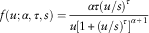
The pdf of the three-parameter Burr distribution is:

(3) $$f(u;\alpha ,\tau ,s)={{\alpha \tau (u/s)^{\tau } } \over {u\left[ {1{\plus}(u/s)^{\tau } } \right]^{{\alpha {\plus}1}} }}$$

where $$\alpha ,\tau \,\gt\, 0$$ are the shape parameters and s>0 a scale parameter, and the pdf of the LN distribution is given by:

(4) $$f(u;\mu ,\sigma )={1 \over {u\sigma \sqrt {2\pi } }}\exp \left( {{\,\minus\,}{{(\log u{\,\minus\,}\mu )^{2} } \over {2\,\sigma ^{2} }}} \right),\quad \quad {\,\minus\,}\infty\,\lt\, \mu \,\lt\, \infty,\sigma \,\gt\, 0.$$

Then the crude claim diagnosis rates, $$\hat{\lambda }_{{x\,:\,\bitheta }} $$ , for this calendar year can be given by:

$$\hat{\lambda }_{{x\,:\,\bitheta }} =N(x\,:\,\bitheta )/{\rm E}^{{\asterisk}} \left( {x\,:\,\bitheta } \right)$$

which has a standard deviation estimated by $$\sqrt {N\left( {x\,:\,\bitheta } \right)} /{\rm E}^{{\asterisk}} \left( {x\,:\,\bitheta } \right)$$ . The estimators can be aggregated over calendar year and/or any of the covariates in θ, if appropriate.

We model the CI diagnosis rates, $${\lambda }_{{x\,:\,\bitheta }} $$ using the following functional form:

$${\lambda }_{{x\,:\,\bitheta }} =\mathop{\sum}\limits_{i=1}^r \kappa _{i} x^{{i{\,\minus\,}1}} {\plus}\exp \left( {\mathop{\sum}\limits_{j=1}^s \delta _{j} x^{{j{\,\minus\,}1}} {\plus}\bibeta \bitheta ^{T} } \right)\quad i=1,\ldots,r,j=1,\ldots,s$$

where κ _i and δ _j are constants and β is a vector of regression coefficients. Note that age x last birthday is a continuous variable so that an estimate of the diagnosis rate at age x exact is given by $$\hat{\lambda }_{{x{\,\minus\,}0.5\,:\,\bitheta }} $$ .

Full details of this methodology can be found in Ozkok et al. (Reference Ozkok, Streftaris, Waters and Wilkie2014a, Reference Ozkok, Streftaris, Waters and Wilkie2014Reference Ozkok, Streftaris, Waters and Wilkieb).

2.2. All-causes rates

Our first model for the investigation of CII diagnosis rates is an all-causes model illustrated in Figure 1.

Figure 1

An all-causes model.

Under this model we assume the policyholder is healthy at the time of commencement of the policy and stays in this state until at some future time he/she transits to insured event. Insured event means diagnosis with a CI or death for FA policies, or diagnosis with a CI for SA policies. This model does not explicitly distinguish between FA and SA policies, but type of policy is included as a possible covariate.

We model $$\lambda _{{x\,:\,\bitheta }} $$ using our two different CDDs: LN and Burr. Recall that the CDDs are used to estimate the missing delays as well as to adjust the exposure in modelling the CI diagnosis rates. Under both CDDs, variable selection results suggest that the best model for all-causes diagnosis rates retain the same variables, namely Smoker status, Policy duration, Office, the Age×Smoker interaction term and Age with the same values for r=0 and s=2. Note that policy type, FA or SA, is not retained as a significant covariate. The methodology we use for variable selection is discussed in Ozkok et al. (Reference Ozkok, Streftaris, Waters and Wilkie2014a, section 5.5), in this paper we employ similar standard stepwise regression techniques using BIC.

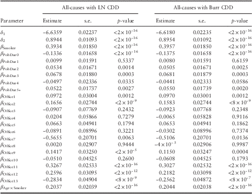
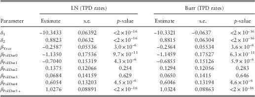
The estimates of the regression coefficients under both CDDs are given in Table 1, together with the standard error of each estimate and its p-value. The parameter estimates under the Burr model are discussed in detail in Ozkok et al. (Reference Ozkok, Streftaris, Waters and Wilkie2014b). We do not repeat these discussions here as the main aim of this paper is to compare the net premium rates under different CDDs. Figure 2 shows a comparison between the estimates of the parameters and 95% confidence intervals of the coefficients under the two models. The estimate of δ ₁ is not shown in the figure for plotting scale purposes. Some confidence intervals for office effect show considerable overlap, suggesting that specific individual offices share common characteristics with regards to resulting CI diagnosis rates. Although combining certain office experiences might provide a simplified model, retaining individual office details is beneficial in cases where specific comparisons are desirable. Table 1 and Figure 2 show that the estimates of the model parameters and their standard deviations are very close to each other under the two CDDs.

Figure 2

Comparison of parameter estimates for all-causes diagnosis rates using Burr and LN CDDs. LN, lognormal; CDD, claim delay distribution.

Table 1

Estimates of parameters for the best model for all-causes diagnosis rates.

Note: LN, lognormal; CDD, claim delay distribution.

Comparisons of all-causes diagnosis rates for non-smokers and smokers using two different CDDs are shown in Figures 3 and 4, respectively. In these figures, weighted rates (Burr or LN) indicate the diagnosis rates obtained by a weighted average of the smoothed rates for all 13 offices where, at each age, the weights are proportional to the adjusted exposure (using Burr or LN CDDs) for each office at that age. Note that the plots are on the log scale with values on the y-axis being on the original scale. For each of the scenarios we also provide the relative diagnosis rates, that is, for a specific characteristic the ratio of all-cause diagnosis rates using the LN CDD to all-cause diagnosis rates using the Burr CDD. The ragged appearance of the relative diagnosis rates (LN/Burr) is owing to weighting the rates by office. The relative diagnosis rates for all scenarios are very close to 1, indicating only small differences between smoothed rates under Burr and LN CDDs. Whether these small differences translate into significant differences in terms of pricing is discussed in section 3.

Figure 3

Comparison of all-cause diagnosis rates for non-smokers estimated by using the CDD under Burr (red-dashed) and LN (black-solid) distributions and relative diagnosis rates. (a) policy duration 0 years; (b) policy duration 5+ years. LN, lognormal; CDD, claim delay distribution.

Figure 4

Comparison of all-causes diagnosis rates for smokers estimated by using the CDD under Burr (red-dashed) and LN (black-solid) distributions and relative diagnosis rates. (a) policy duration 0 years; (b) policy duration 5+ years. LN, lognormal; CDD, claim delay distribution.

2.3. Sensitivity of CI diagnosis rates to CDD estimates

In the claims data set, 17% of the claims have a missing date of diagnosis. As all these claims have a date of settlement, we can estimate their dates of diagnosis using the CDD. More specifically, for each missing observation the analysis presented so far uses the median of the posterior distribution of the delay to estimate missing dates of diagnosis (Ozkok et al., Reference Ozkok, Streftaris, Waters and Wilkie2012). Here we investigate the effect of using different percentiles of the CDDs on the estimates of CI diagnosis rates. Once the model coefficients are estimated, the fitted number of claims, thus the fitted diagnosis rates ( $$\tilde{\lambda }_{{x\,:\,\bitheta }} $$ ) can be calculated. To obtain a confidence interval for diagnosis rates we use parametric bootstrap methodology (Efron & Tibshirani, Reference Efron and Tibshirani1993). More specifically, we first simulate 500 samples assuming

$$N^{{{\rm sim}}} \left( {x\,:\,\bitheta } \right)\,\sim\,\:\;{\rm Poisson}\left( {\tilde{\lambda }_{{x\,:\,\bitheta }} \;{\rm E}^{{\asterisk}} \left( {x\,:\,\bitheta } \right)} \right)$$

and then fit the model described in equations (1)–(5) to obtain an empirical sampling distribution of $$\lambda _{{x\,:\,\bitheta }} $$ .

Each panel of Figure 5 shows the following information for non-smokers and for policy duration either 0 or 5+ years:

• ∙ The 95% confidence intervals for the diagnosis rates, relative to the diagnosis rates themselves, calculated using the median of the CDD to estimate missing dates of diagnosis, for each of the two CDDs: red (Burr) and black (LN).

• ∙ The diagnosis rates using the 97.5% point of the CDD to estimate missing dates, relative to the diagnosis rates using the median of the CDD, for each CDD: light green (Burr) and green (LN).

• ∙ The diagnosis rates using the 2.5% point (panels (c) and (d)) of the CDD to estimate missing dates, relative to the diagnosis rates using the median of the CDD, for each CDD: light blue (Burr) and blue (LN).

Figure 5

Sensitivity analysis for non-smokers using 95% confidence interval (CI) of the CDD under Burr and LN distributions. (a and c) policy duration 0 years; (b and d) policy duration 5+ years. LN, lognormal; CDD, claim delay distribution.

The principal features of Figure 5 are the same for the two CDDs. For panels (b)–(d), the estimated diagnosis rates using the 97.5% or 2.5% point of the CDD to estimate missing dates of diagnosis lie within the 95% confidence intervals, but this is not the case for policy duration 0 when we use the 97.5% point of the CDD (see panel (a)). However, it is the case if we use a percentage point of the CDD between 2.5% and 95%. See Ozkok et al. (Reference Ozkok, Streftaris, Waters and Wilkie2014b) for more discussion of this in relation to the Burr CDD.

2.4. An alternative all-causes model

All-causes diagnosis rates can be modelled using an alternative approach illustrated in Figure 6. This model allows separately for transition from healthy to diagnosis with a CI ( $$\lambda _{{x\,:\,\bitheta }}^{{{\rm CI}}} $$ ), which would result in a claim under an FA or an SA policy, and transition from healthy to dead ( $$\lambda _{{x\,:\,\bitheta }}^{{\rm D}} $$ ), which would result in a claim under an FA, but not an SA, policy.

Figure 6

An all critical illness (CI) causes and death model.

The best models for the diagnosed with CI rates, $$\lambda _{{x\,:\,\bitheta }}^{{{\rm CI}}} $$ , retain the same variables using the Burr and the LN CDD, namely Sex, Smoker status, Benefit type, Policy duration, Office, the Age×Smoker interaction term and Age with the same values for r=0 and s=2 in equation (5). The estimates of the model coefficients under the Burr and LN CDDs are given in Table 2, together with the standard error of each estimate and its p-value.

Table 2

Estimates of parameters for the best model for $$\lambda _{{x\,:\,\theta }}^{{{\rm CI}}} $$ .

Note: LN, lognormal.

We note that under this model the significant variables are different from the ones under the all-causes model given in section 2.2 with policy type having a significant positive effect. That is, when we exclude death claims, the difference between FA and SA rates is significant with SA rates being higher. Under this model Sex also appears as a significant covariate with lower CI diagnosis rates for males. We think this is because of higher cancer rates for women owing to high breast cancer rates. When we include death rates as in section 2.2, higher mortality rates for males cancel out higher cancer rates for females and Sex is not a significant covariate in the model.

2.5. Cause-specific rates

We can use our methodology to estimate diagnosis rates for individual causes. The question of interest here is whether type of CDD used affects significantly the estimated diagnosis rates. We investigate this in relation to two large causes – cancer and heart attack – and three small ones – multiple sclerosis (MS), major organ transplant (MOT), and total and permanent disability (TPD).

The best models for these individual causes, except cancer, retain the same covariates under both CDDs. For cancer the best models under the Burr CDD and the LN CDD have different covariates, namely:

• Burr CDD: Age, Sex, Smoker, Year, Age×Smoker.

• LN CDD: Age, Sex, Office and Policy type.

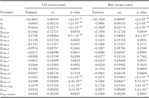
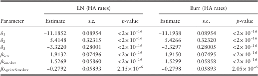
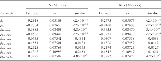
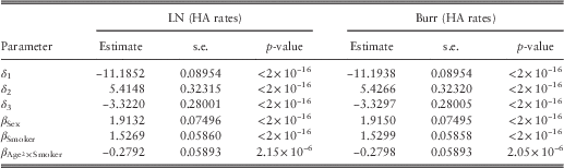
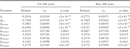
In order to compare cancer diagnosis rates under the two different CDDs, we use models that include all these variables: Age, Sex, Smoker, Year, Office, Policy type and Age×Smoker. The parameter estimates for the models for cancer diagnosis rates are set out in Table 3. The parameter estimates for the models for diagnosis rates for the other four causes are set out in Tables 4–7.

Table 3

Estimates of the parameters for the model for cancer diagnosis rates.

Note: LN, lognormal.

Table 4

Estimates of the parameters for the model for heart attack (HA) diagnosis rates.

Note: LN, lognormal.

Table 5

Estimates of the parameters for the model for multiple sclerosis (MS) diagnosis rates.

Note: LN, lognormal.

Table 6

Estimates of the parameters for the model for major organ transplant (MOT) diagnosis rates.

Note: LN, lognormal.

Table 7

Estimates of the parameters for the model for total and permanent disability (TPD) diagnosis rates.

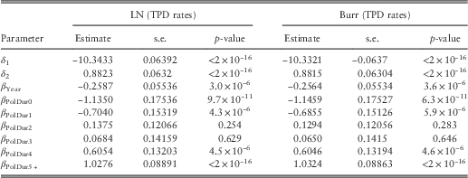
Note: LN, lognormal.

Comparisons of cancer, heart attack and MS diagnosis rates for male non-smokers estimated using the two different CDDs are shown in Figures 7, 8 and 9, respectively. In addition, comparisons of MOT and TPD rates for policy duration 5+ estimated using the two different CDDs are shown in Figures 10 and 11, respectively. In these figures DR (under Burr or LN CDD) denotes the diagnosis rates estimated by using the appropriate CDD. In Figures 7, 9 and 11, DR (under Burr or LN CDDs) indicate the diagnosis rates obtained by a weighted average of the smoothed rates at each age. The crude rates and the confidence intervals of the crude rates (under Burr or LN CDD) can also be seen in the figures. These plots are on the log scale with values on the y-axis being on original scale.

Figure 7

Comparison of cancer rates for male non-smokers estimated by using the CDD under Burr and LN distributions and relative diagnosis rates. LN, lognormal; CDD, claim delay distribution.

Figure 8

Comparison of heart attack rates for male non-smokers estimated by using the CDD under Burr and LN distributions and relative diagnosis rates. LN, lognormal; CDD, claim delay distribution.

Figure 9

Comparison of multiple sclerosis rates for male non-smokers estimated by using the CDD under Burr and LN distributions and relative diagnosis rates. LN, lognormal; CDD, claim delay distribution.

Figure 10

Comparison of major organ transplant rates estimated by using the CDD under Burr and LN distributions and relative diagnosis rates. LN, lognormal; CDD, claim delay distribution.

Figure 11

Comparison of total and permanent disability rates for policy duration 5+ estimated by using the CDD under Burr and LN distributions and relative diagnosis rates. LN, lognormal; CDD, claim delay distribution.

For each cause we also provide the relative diagnosis rates, that is, for a specific characteristic, the ratio of the all-causes diagnosis rates using the LN CDD to the all-causes diagnosis rates using the Burr CDD. The ragged appearance of the relative diagnosis rates (LN/Burr) in some cases is owing to the weighting. The figures indicate that the difference between smoothed rates under Burr and LN CDDs is <5% for almost all cases we have investigated. The only exception is MOT showing a difference of nearly 10%. However, for this case we have very few data leading to models where only the constant is significant.

3.1. Formulae

In this section, we set out generic formulae for the calculation of a net premium. We will use these formulae to price a CII policy that covers “all-causes” using the model given in Figure 1, and a FA and a SA policy using the model given in Figure 6. We also consider an “all-causes except TPD” model as this product is sold in the UK market. In each case, $$\lambda _{{y\,:\,\bitheta }}^{{}} $$ denotes the total transition intensity of the diagnosis of a CI at exact age y with covariates θ.

For convenience, the initial age x, and the term n, of the policy will always be integers. We will assume, as is often the case in practice, that premiums are paid monthly in advance during the term of the policy while the life is healthy. The expected present value (EPV) of an annuity of annual amount 1 payable monthly while in the “healthy” state from age x for a maximum of n years is denoted $$\ddot{a}_{{x\,:\,\left. {\overline{\, n \,}}\! \right&#x007C; }}^{{(12)}} $$ . Any premiums paid between diagnosis and settlement are likely to be refunded. For convenience, we will assume that the benefit is paid at the end of the month, measured from the issue of the policy, in which diagnosis occurs. The EPV at age x for a healthy life of a payment of 1 on the occurrence of an insured event (diagnosis with a CI or, possibly, death) within n years is denoted $$A^{{(12)1}} _{{x\,:\,\left. {\overline{\, n \,}}\! \right&#x007C; }} $$ . In practice, the average observed delay between diagnosis and settlement of a CI claim is around 6 months and can be much longer. We have not allowed for this delay in the calculation of the net premium because at least one major insurer in the United Kingdom will pay interest if settlement is significantly delayed beyond diagnosis, for example, by more than 2 months, and we suspect other insurers would do the same.

The probability that a life healthy at age x will remain healthy until at least age x+t is denoted $$_{t} p_{x} $$ .

We use a fixed interest rate i per year, with $$v=1/(1{\plus}i)$$ , $$d^{{(12)}} =12(1{\,\minus\,}(1{\plus}i)^{{{\minus}1/12}} )$$ and $$\delta =\log (1{\plus}i)$$ . Unless otherwise stated, we use an interest rate of 3% per annum.

We calculate the annual amount of net premium, $$P_{{x:\left. {\overline{\, n \,}}\! \right&#x007C; }}^{{}} $$ , for unit benefit as follows:

(6) $$P_{{x:\left. {\overline{\, n \,}}\! \right&#x007C; }} =A_{\quad\ \,{\:\:\:\:\:\:\:\:\:\:\:x\,:\,\left. {\overline{\, n \,}}\! \right&#x007C; }}^{{(12)1}} /\ddot{a}_{{x\,:\,\left. {\overline{\, n \,}}\! \right&#x007C; }}^{{(12)}} $$

where

$$A_{\quad\ \,\,{\:\:\:\:\:\:\:\:\:\:\:x:\left. {\overline{\, n \,}}\! \right&#x007C; }}^{{(12)1}} =1{\,\minus\,}d^{{(12)}} \ddot{a}_{{x:\left. {\overline{\, n \,}}\! \right&#x007C; }}^{{(12)}} {\,\minus\,}v^{n} \,_{n} p_{x} $$

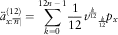$$\ddot{a}_{{x:\left. {\overline{\, n \,}}\! \right&#x007C; }}^{{(12)}} =\mathop{\sum}\limits_{k=0}^{12n{\,\minus\,}1} {1 \over {12}}\:\:v^{{{k \over {12}}}} \:\,_{{{k \over {12}}}} p_{x} $$

and

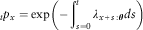(7) $$_{t} p_{x} =\exp \left( {{\minus}\mathop{\int}\nolimits_{s=0}^t \lambda _{{x{\plus}s\,:\,\bitheta }} \:ds} \right)$$

Values of $$_{t} p_{x} $$ can be calculated from equation (7) using numerical integration. However, the models summarised in Tables 1 and 2 include policy duration as a significant covariate. Policy duration is measured as curtate duration from the diagnosis of the policy, split into curtate durations 0, 1, 2, 3, 4 and 5 or more years. As there are different parameters for each of these durations, it is not possible to convert these models into models with policy duration as a continuous variable. This means care must be taken with the integration in equation (7), recognising the discontinuities at integer durations up to 5 years.

3.2. Net premium rates for all-causes

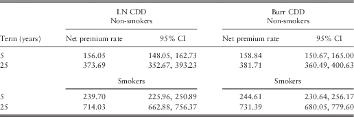
In this section, we obtain the net premium rates for the model summarised in Table 1 and Figures 2–4. Figure 12 shows net premiums for all-causes CII for different terms for a 40-year-old policyholder with a £100,000 benefit amount. For such a 5-year CI and death cover, the net premium that a non-smoking policyholder pays £156.05 (95% confidence interval: £148.05, £162.73) using the LN CDD and £158.84 (£150.67, £165.00) using the Burr CDD. The small difference between net premiums and the narrow confidence interval increase with increasing term time. For example, when the insurance cover is increased to 25 years the net premium amounts change to £373.69 (£352.67, £393.23) (LN CDD) and £381.71 (£360.49, £400.63) (Burr CDD). The net premium rates for a corresponding smoker are given in Table 8. These figures show that as the term increases, the confidence intervals get wider owing to the higher uncertainty. However, in all cases the net premium rates calculated under different CDDs lie within each other’s confidence intervals.

Figure 12

Net premiums for all-causes for a 40-year-old policyholder with £100,000 benefit amount using the CDD under Burr and LN distributions. (a) Non-smokers; (b) Smokers. LN, lognormal; CDD, claim delay distribution and CI, confidence interval.

Table 8

Net premium rates and their confidence intervals for a 40-year-old policyholder with £100,000 benefit amount using the CDD under Burr and LN distributions.

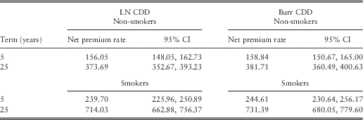
Note: CDD, claim delay distribution; LN, lognormal; CI, confidence interval.

3.3. Sensitivity of net premium rates to interest rate

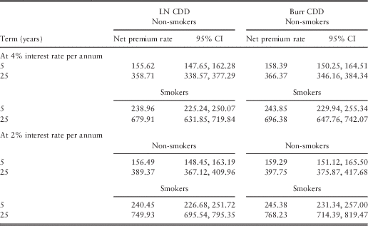
Our net premium calculations in Table 8 are based on a 3% interest rate. The sensitivity of net premium rates to the interest rate by changing it by 1% can be seen in Table 9. The important conclusion remains unchanged: the choice of CDD does not significantly affect the net premium rate in the sense that in all cases the net premium rate for each CDD lies within the 95% confidence interval for the net premium rate calculated using the alternative CDD (Figures 13 and 14).

Figure 13

Net premiums for all-causes for a 40-year-old policyholder with £100,000 benefit amount using the CDD under Burr and LN distributions at 4% interest rate per annum. (a) Non-smokers; (b) Smokers. LN, lognormal; CDD, claim delay distribution and CI, confidence interval.

Figure 14

Net premiums for all-causes for a 40-year-old policyholder with £100,000 benefit amount using the CDD under Burr and LN distributions at 2% interest rate per annum. (a) Non-smokers; (b) Smokers. LN, lognormal; CDD, claim delay distribution and CI, confidence interval.

Table 9

Net premium rates for all-causes for a 40-year-old policyholder with £100,000 benefit amount using the CDD under Burr and LN distributions at 4% and 2% interest rates per annum.

Note: LN, lognormal; CDD, claim delay distribution; CI, confidence interval.

3.4. Net premium rates for FA and SA policies

We can calculate the net premium rate for a FA CII policy using the model given in Figure 6. The first part of the calculation is to obtain the net premium rates for a FA CI with “death only cover”. Although this does not correspond to any product sold in the market, it is interesting to consider as shown later. Having done this, we need to add the net premium for the “critical illness only (excluding death)” cover. The latter calculation uses the parameter values in Table 2 with policy type set to FA.

For a 40-year-old male policyholder and £100,000 benefit amount the net premium rates for “death only” cover are shown in Figure 15. Higher diagnosis rates for smokers lead to significantly higher net premium rates. However, the interesting point in this figure is that the point estimates of net premium rates are marginally outside the CIs of the rates using a different CDD. This indicates that the choice of CDD has had a significant effect on the net premium rate, albeit for a policy not available in the market.

Figure 15

Net premiums for only death cover for 40-year-old males with £100,000 benefit amount using the CDD under Burr and LN distributions. (a) Non-smokers; (b) Smokers. LN, lognormal; CDD, claim delay distribution and CI, confidence interval.

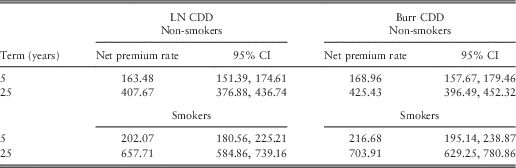
Figure 16 shows the net premium rates for an FA policy (death and CI included) using our two different CDDs. The differences in net premium rates are now not statistically significant: in each case, the net premium calculated using one CDD lies within the 95% confidence interval of the net premium calculated using the other CDD. The confidence intervals for net premium rates for smokers are wider than those for non-smokers as we have far less data for smokers (Table 10).

Figure 16

Net premiums for a full accelerated policy for 40-year-old males with £100,000 benefit amount using the CDD under Burr and LN distributions. (a) Non-smokers; (b) Smokers. LN, lognormal; CDD, claim delay distribution and CI, confidence interval.

Table 10

Net premium rates for full accelerated policies and their confidence intervals (CIs) for 40—year-old males with £100,000 benefit amount.

Note: LN, lognormal; CDD, claim delay distribution.

We can calculate net premium rates for an SA policy using the model in Figure 6 and the parameter values in Table 2, with policy type set to SA. The significant positive coefficient for policy type indicates higher diagnosis rates, for all causes other than death, for an SA policy compared with an FA policy. Figure 17 shows the net premiums for an SA policy with £100,000 benefit amount using the Burr and LN CDDs and the corresponding 95% confidence intervals for a 40-year-old male non-smoker and smoker. Based on this figure we can conclude that the two sets of net premiums are not significantly different from each other.

Figure 17

Net premiums for a stand alone policy for 40-year-old males with £100,000 benefit amount using the CDD under Burr and LN distributions. (a) Non-smokers; (b) Smokers. LN, lognormal; CDD, claim delay distribution and CI, confidence interval.

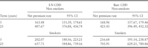
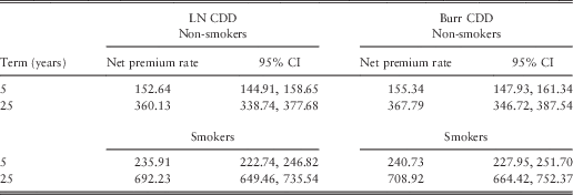
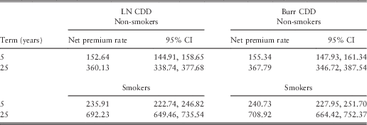
Finally, we present the net premium rates for a CI policy that does not cover TPD. This is a product which does exist in the UK market. Note that neither Sex nor policy type is significant for this model. The net premium rates for this policy for a 40-year old under different CDDs are shown in Figure 18. Net premium rates for policies with a term of 5 or 25 years are shown in Table 11, together with their 95% confidence intervals. As expected, the net premiums are slightly lower than the net premiums calculated for all-causes (see Figure 12; Table 8). However, the effect of using different CDDs is not significant.

Figure 18

Net premiums for all-causes except TPD for 40-year-old policyholders with £100,000 benefit amount using the CDD under Burr and LN distributions. (a) Non-smokers; (b) Smokers. TPD, total and permanent disability; LN, lognormal; CDD, claim delay distribution and CI, confidence interval.

Table 11

Net premium rates for policies covering all-causes except TPD and their confidence intervals (CIs) for a 40-year-old policyholder with £100,000 benefit amount.

Note: LN, lognormal; CDD, claim delay distribution.