YOUTH EMPLOYMENT AND THE FAMILY ECONOMY

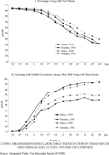
Although more attention is focused on the young children who worked and who became the targets of anti–child labor and compulsory schooling campaigns, most “working children” were sons and daughters in their late teens or early twenties. Figure 1 presents data from the 1910 and 1920 federal censuses on the fraction of urban youth living with one or both parents (panel A), and the fraction of such youth who had gainful occupations (panel B). Most sons and daughters entered the labor market in their mid- to late-teens but remained in their parents' households until their early twenties. Many, in fact, remained at home until they married.⁷

Most individuals, therefore, spent a number of years living at home yet earning incomes.

Today, too, entry into the labor market generally precedes departure from home. But, whereas today the earnings of working children are viewed as the property of the children, in the past, those earnings were viewed as the property of the parents. Working children turned over most, or all, of their earnings to their parents. Tamara Hareven argues that among workers at the Amoskeag Mill in Manchester, New Hampshire this custom was an “unwritten law.”⁸

In a 1903 survey conducted by the New Jersey Bureau of Statistics of Labor and Industries, 814 out of 943 workers between the ages of 12 and 19 surveyed reported giving all of their earnings to their parents, and another 45 gave over two-thirds of their earnings to their parents.⁹ Even sons and daughters in their twenties turned over most of the contents of their pay envelopes to their parents. A 1907 survey found that over half of all women in their late twenties and living at home contributed all of their earnings to their parents.¹⁰

Because of this practice, youth employment during this period tends to be studied in terms of its contributions to the family economy. Historians have argued that sending children into the labor market was a “family strategy” for keeping the family out of poverty or debt in the face of hardships such as the low earnings, unemployment, or absence of the father.¹¹

Michael Haines has also emphasized the importance of income from children in the later stages of the family life cycle. Using data from the Cost of Living survey of 1889/90, Haines showed that income from the family head peaked when the head was in his 30s whereas family expenditures peaked when the head was in his 50s. The gap between the head's earnings and family expenditures in these later stages was filled by the earnings of working children.¹²

The model of household decision making underlying these studies is the neoclassical, or so-called unitary, model of the household in which the household maximizes a household welfare function subject to a unified budget constraint that pools income from all sources. This model abstracts from the potential conflicts between household members' objectives. Household members are assumed to work together to maximize the welfare of the household as a whole, and the rewards to children's work are shared by all household members in the form of a more relaxed budget constraint.

The one study that considers the returns to work to the working children themselves, concludes that these returns were very small. Donald Parsons and Claudia Goldin argue that compensation of working children could have taken the form of transfers of physical assets when the children reached adulthood.¹³

But using the same data as Haines, the 1889/90 Cost of Living survey, they find that the savings rate out of children's income was no different than the savings rate out of all other family income. Families with working children did not accumulate assets at a faster rate than families without working children. This finding, together with the low rate of retained earnings of working children, lead Parsons and Goldin to conclude that, “there is little evidence … to suggest that offspring who worked as youths were compensated with greater physical asset endowments.”¹⁴

What incentives, then, did children have to work? The standard answers are altruism and the threat of punishment. These factors were clearly important. Many youth workers were keenly aware of the importance of their earnings to the welfare of their families. Marie Proulx, who began working at the Amoskeag Mill as a teenager, explained her situation as follows:

Similar sentiments were expressed by a man who grew up in the Polish community in Pittsburgh in the early 1900s: But other evidence suggests that altruism by children was not enough. Louise Montgomery in her 1913 study of girls in the Chicago stockyards district observed that when doing piecework, some girls refused to go beyond a “comfortable speed limit” and some even “found a pleasurable excitement in discovering just how ‘comfortable’ they could be without losing their position.” In response, mothers would often give “additional incentive to increased speed” by tying spending money and even funds for necessary clothing to the girls' earnings.¹⁷ Esther Little and William Cotton encountered similar schemes in the Kensington neighborhood of Philadelphia. One mother they encountered was afraid her sons, ages 17 and 19, would not be willing to work unless she gave them plenty of spending money. She therefore gave them 15 cents on every dollar they earned as well as many “extras.”¹⁸

Such “bribes” indicate that children's income altered how a household allocated its resources, but do not necessarily imply that children gained more power in the household. Other evidence, though, indicates that working changed the status of the child in the household. Charles Oliver, a clerk at the First National Bank in Philadelphia in the 1930s, described the change in treatment he received after he started working:

Woods and Kennedy emphasized how working changed girls' attitudes, noting girls' sentiments that they “could do what they please” and that “they shouldn't be restrained.”²⁰ But Woods and Kennedy also claimed that the household changed in relation to the girl. Echoing the words of Oliver, they reported that when a girl became a wage-earner she was less likely to be subjected to physical punishment.²¹

Part of this change in status appears to have been greater input into household decision making. In particular, working children had some influence on how the contents of their pay envelopes were spent. Montgomery found that 290 of the 300 girls ages 16 to 24 whom she interviewed in the Chicago stockyards district had “no independent control of their own wages.”²²

But she goes on to note that working girls voiced their opinions as to how their earnings should be allocated: These conflicts often led to changes in household spending patterns. Montgomery argues: In other words, children's remittances and parental authority were not predetermined but rather were the outcome of negotiations between parents and children.

The idea that family decisions are the outcome of bargaining among household members is not new. Marilyn Manser and Murray Brown and Marjorie McElroy and Mary Jean Horney proposed bargaining models of household decision making over 20 years ago.²⁵

In the intervening years, other collective models of the household have followed, accompanied by a number of empirical tests that have shown that the sources, and not just the sum total, of household income influence household consumption decisions.²⁶ But these models and tests have focused on the interactions between husbands and wives. Can collective models of the household be extended to describe the interactions between parents and adolescents in the early twentieth century? Skepticism that children could have participated in household decision making during this period is perhaps best expressed in the language of a bargaining model: what were the children's threat points? In most models of bargaining between husbands and wives, the assumed threat point is exit: if negotiations break down, the relationship can be dissolved through separation or divorce. In the context of parent-child relationships in the early twentieth century, exit only became an option in late adolescence.

But exit need not be the only threat point. Shelly Lundberg and Robert Pollak have proposed that an alternative threat point is simply noncooperation.²⁷

Children could have simply refused to work or to have shirked on the job in such a way as to reduce earnings and increase their chances of being fired. Montgomery's account of pieceworkers in Chicago is a case in point. Montgomery's study also suggests an alternative noncooperative outcome: the establishment of a formal boarding arrangement between the parent and child. She found that conflicts between parents and sons sometimes led to arrangements in which the sons paid fixed sums for their board and lodging and retained control over their remaining income. Although this arrangement was fairly uncommon for daughters, Montgomery met ten girls for whom the conflict had “reached a climax” and had consequently “demanded and secured an equal right with the brother to pay a fixed sum for board.”²⁸

The difference Montgomery observed between the experiences of sons and daughters could itself be interpreted as further evidence of bargaining between parents and children. Although some single women lived on their own in boarding houses or similar arrangements in the early twentieth century, the exit options for daughters were far more circumscribed than those of sons. For daughters, the most common route out of the parental household was through marriage. In addition, daughters tended to earn less than sons, which limited opportunities. In the context of a bargaining or collective model of the household, these factors should have led daughters to have less influence in household decisions than sons. Data on retained earnings seem to bear this out. In the 1903 New Jersey study of workers ages 12 to 19, 91 percent of girls compared to 82 percent of boys turned over all their income to their parents. Some of this difference was due to the difference in earnings levels between boys and girls, but not all of it. Even after controlling for weekly earnings, girls were 5 percentage points more likely to contribute all their income to their parents than were boys.²⁹

THE BUREAU OF LABOR STATISTICS COST OF LIVING SURVEY OF 1917–1919

The discussion in the previous section suggests that children's entry into the labor market affected a wide variety of household behaviors including the rules regulating the leisure activities of children and even the use of corporal punishment. Such changes in social relations are, however, difficult to quantify, and the only information available on these issues takes the form of the qualitative accounts described above. The empirical analysis here focuses on a more easily quantified aspect of household behavior: household expenditures. Household expenditures represent only a subset of household decisions, albeit a fairly important one. How a household allocates its resources has important implications for the welfare of its members. Moreover, as Montgomery's observations of Chicago households reveal, this was a key area of potential conflict between parents and working children.

The data employed in the analysis come from the Cost of Living Survey of 1917–1919 conducted by the Bureau of Labor Statistics.³⁰

These data were collected to construct the original weights of the Consumer Price Index. Hence, they include expenditures for a broad range of goods. But what makes them particularly rich for this study is that they include a measure of private consumption—clothing expenditures—as well as information on the labor supply, wages, and total earnings, for each member of the household. The predecessor to the Department of Labor, the Commissioner of Labor, had conducted cost of living surveys in 1889/90 and 1901. However, while these surveys were somewhat similar in scope, they do not permit the kind of analysis required to examine the hypothesis of interest. For example, all that is available for the 1901 survey are state-level averages; the original family survey data have been lost. Family-level data for the 1889/90 survey survive, but this survey only collected data on the number of working children, total income from children and total expenditures on children's clothing. These data, therefore, cannot be used to examine how an individual child's private consumption varied with her labor market outcome.³¹

The timing of the 1917–1919 data would seem to be problematic for two reasons. First, the employment of child labor had been on the decline for several decades and in the first two decades of the 1900s had become increasingly regulated and restricted. But, as noted previously, most of the working children in families were sons and daughters in their late teens and early twenties and thus unaffected by these changes. However, the labor market behavior of adolescents did change in the first half of the twentieth century with the expansion of secondary education. The school enrollment rates of 14 to 17 year olds rose from 18 to 73 percent between 1910 and 1940.³²

Even so, by 1920 still less than a third of 14 to 17 year olds were in high school, and the school enrollment rates of youth 18 and over were still very low. The more dramatic changes in youth school enrollment and labor market participation took place after 1920. In some ways, the 1917–1919 data represent one of the last snapshots of family consumption behavior in the era when children rather than mothers were the most important group of supplementary earners.

The second reason the timing seems problematic is that for much of the survey period, the United States was at war. However, very little rationing of domestic consumers took place in the United States during the First World War. Some restrictions were placed on consumer purchases, but these did not involve restrictions on the total quantities of goods that a household could purchase.³³

Prices rather than quantity constraints allocated scarce goods across consumers. Another consequence of the war, in fact, makes this period ideal for addressing the question at hand. This was a period of high labor demand and very low unemployment. In this labor market, those who wanted jobs were generally able to find jobs. Young women's labor market opportunities, in particular, expanded during the war. Some lingering effects of this can be seen in Figure 1: the percentages of young women ages 17 to 24 with gainful occupations were 8 to 9 points higher in 1920 than in 1910.

The Cost of Living data were collected through interviews with the households of wage earners and low- and medium-salaried workers in 99 “industrial centers” in 1918 and 1919. These industrial cities embraced all regions of the country and ranged in size from the largest cities of the time, New York City and Chicago, to small one-industry towns such as the mining town of Pana, Illinois, which had a population of 6,122 in 1920. Most, however, were large: 47 had populations of over 100,000 and an additional 31 had populations of over 25,000 in 1920.³⁴

Interviews were organized by cities and were staggered over a couple of years so that the data cover different annual periods between 31 July 1917 and 28 February 1919. All of the survey periods, though, overlap for the period from 28 February 1918 to 31 July 1918. Households were interviewed only once and were asked for all their earnings and expenditures over the specified year-long period. The data, therefore, suffer from some degree of recall bias. Such bias would expected to be relatively small, however, for clothing expenditures because such expenditures tend to be “lumpy,” taking place fairly infrequently and being large relative to other types of expenditures.

Surveyed households were not randomly selected from the interview cities. To be included in the survey, households had to contain an intact married couple and at least one child. Other selection criteria served to exclude the upper and lower tails of the income distribution. The survey specifically excluded “slum or charity families” and non–English speaking families who had resided fewer than five years in the United States, and required that at least 75 percent or more of a household's total income come from family labor earnings.³⁵

Particularly important for this study, the survey required that all family members contribute all their earnings to “the family fund.” Households in which children had boarding arrangements with their parents, like those described by Montgomery were excluded.³⁶ However, as discussed above, the vast majority of sons and daughters living at home contributed all their earnings to their parents. The survey also required that households reside in the same locality for the entire year covered in the survey and be able to provide all items of expenditure and income of household members other than those living as lodgers.³⁷

Over 12,000 households participated in the survey. The sample, however, was skewed toward younger families, so only about a third of the surveyed households contained sons and daughters age 12 or older.³⁸

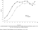
Figure 2 presents the labor market participation rates of the sons and daughters ages 12 to 24 of the surveyed households. Here, labor market participation is defined as having positive labor earnings. These rates are generally higher than the census-based “gainful occupation” rates of urban children living with one or more parents presented in Figure 1. The differences are due primarily to the differences in the definitions of market participation. The “gainful occupation” definition imposes a high standard for participation and hence, misses many young workers who may have worked sporadically or did odd jobs rather than working regularly scheduled hours. This explains why the differences between the Cost of Living and census data participation rates are largest at the youngest ages. But some of the disparity, particularly for older daughters, is likely due to the increased wartime demand for labor.

A notable feature of Figure 2 is the drop in labor market participation rates for sons between ages 21 and 23. This highlights an issue that must be kept in mind in the empirical analysis that follows. The sons and daughters observed living with their parents represent a self-selected group of all sons and daughters. This is particularly true of those in their twenties as half of their peers had already left their parents' homes. It is unclear, however, in which direction such selection effects would go. Sons and daughters who stayed at home into their twenties may have been those with the worst outside opportunities. The young men still at home during the survey years would have also included those found to be unfit to serve in the armed services during the war. The dip in employment rates for sons in the their early twenties may reflect such negative selection. But those who remained at home may have also been those whose preferences conflicted the least with those of their parents or who received the most favorable treatment from their parents.

METHODOLOGY

An intuitive approach to examining how an individual's labor market outcomes affected her influence in household expenditure decisions would be to address the following question: did expenditures on an individual's private consumption goods vary with that individual's labor market outcomes? Clothing expenditures are a natural choice as a measure of private consumption because they can generally be assigned to a particular individual within a household, and, on average, they represent a sizable fraction of total private consumption. One could estimate a demand function for an individual's clothing expenditures that includes variables implied by a unitary household model—household income, household demographics, relative prices—as well as measures of the individual's labor market outcome such as an indicator for labor market participation or her wage. Under the null hypothesis that individual labor market outcomes had no effect on household expenditure decisions, the coefficients on those variables should be equal to zero.³⁹

This is the basic intuition behind the tests used by Martin Browning and his co-authors in their study of the bargaining between husbands and wives in Canadian households in the 1980s.⁴⁰ This approach, however, is problematic when looking at how work affected the influence of children in household decision making.

The first challenge arises from the fact that adding children as potential decision makers greatly increases the complexity of the bargaining problem. The bargaining power of any one decision maker in the household will depend on her position relative to all other decision makers in the household. When only husbands and wives are assumed to be the decision makers, all that matters is the position of the wife relative to the husband (or vice versa). But when children are allowed to be decision makers, the dimensionality of the problem increases. The bargaining power of a particular child will depend not only on her position relative to her father's, but also on her position relative to her mother's position, her position relative to the positions of other children in the household, and the positions of those other household members to each other. Moreover, this dimensionality will vary from household to household.

The second challenge is that the presence of working children in a household was likely correlated with other household characteristics that may also have affected household expenditure patterns. In other words, children's labor supply decisions were endogenous to household expenditure decisions. Such correlations fit into both the unitary and collective household models. In both frameworks, the decision to send children into the labor market depends on the difference in the utility level when children were working and the utility level when children were in school or in the home. Observable household characteristics such as size will affect this decision as well as influence household expenditure choices. More problematic, unobservable characteristics will also produce such correlations. For example, families with greater preferences for adult goods relative to their children's welfare would have been more likely to have had children working as well as having had lower expenditures on children's goods. Moreover, the collective models suggest an additional explanation of a correlation between the presence of working children and spending patterns: if working gave children more influence in household consumption decisions, then the children with the greatest incentives to work would be children whose preferences were the most in conflict with the preferences of their parents.

These dimensionality and endogeneity issues make using variation across households to identify the effect of labor market status on children's influence in household decision making problematic. Therefore, the approach employed here is to use variation within households to identify this effect. In other words, the empirical question examined is: within a given household, did the expenditures on children's clothing vary with those children's labor market outcomes? This is accomplished by including household fixed effects in the demand equations. Household fixed effects will capture all characteristics common to the household. These include the factors usually included in demand functions such as total household expenditure or income, household demographics, and relative prices as well as unobservables such as the relative bargaining power of the mother to the father and parents' relative preferences for adult and children's goods. Any variation that remains will have to be explained by variation in the characteristics of children within a given household.

I consider three different labor market status measures: an indicator for whether a child was working or not; the child's total annual earnings; and the child's weekly wage rate. Each of these measures can be thought of as testing slightly different versions of the household bargaining hypothesis. The work indicator variable provides the most direct test of Woods and Kennedy's proposition that entering the labor market brought a child more power within the household. The earnings measures test hypotheses that assert that expenditures on a child's private consumption goods were tied in some direct way to the child's contributions to the household. For instance, parents may have simply returned some fraction of the child's earnings back to the child either directly or through expenditures on her private goods. The most straightforward test of this is to look at the effect of total annual earnings on annual clothing expenditures. The problem with this approach, though, is that annual earnings represent the interaction between the wage rate and labor supply choices. So to see if potential earnings matter in a different way from actual earnings, I also consider the effect of a child's weekly wage rate on her clothing expenditures.

The empirical models also include age and gender, characteristics that, as discussed previously, may have also been correlated with potential bargaining power. But here it is important to discuss a weakness of using clothing expenditures as a measure of the outcome of bargaining within the household. Clothing expenditures are only one component of private consumption. If the preferences for clothing relative to other goods varies with a particular characteristic, then these data will not be very informative as to how bargaining power varied with that characteristic. For instance, if daughters had stronger preferences for clothing relative to other goods than did sons, observing higher expenditures on daughters' clothing will not necessarily be evidence of daughters having more influence in household decision making.

The sample is restricted to sons and daughters ages 12 to 24. Due to the use of household fixed effects, the sample is further restricted to those children who had one or more siblings in this age group. These are the only observations which will be used to identify the effects of the other variables. Limiting the sample in this way, therefore, makes the reported sample means and sizes more informative of the data actually used to estimate the parameters of interest.

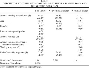
The sample consists of 5,192 sons and daughters from 2,076 families. Table 1 presents some descriptive statistics for the sample. Half of the sons and daughters in the sample were at work at some time during the survey year. Among those who worked, the mean weekly wage was $9.68, less than half the weekly wage rate of their fathers. Their average annual earnings were $338.37 and accounted for, on average, 17 percent of their households' incomes. Working children were older and were more likely to be male than those who did not work. They also had, on average, higher clothing expenditures.

RESULTS

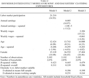
Table 2 presents the results from the fixed effects models using the three different measures of labor market outcome. The models include squared terms for wages, earnings, and age to allow for nonlinear effects of these variables.⁴¹

All three models indicate that working led to rewards in terms of personal clothing expenditures. The first specification looks at the effect of working versus nonworking. Expenditures on clothing for sons and daughters who worked in the market were $21 higher than the expenditures on clothing for their nonworking siblings. This represents a substantial bonus given that the sample mean of clothing expenditures was $69. It also translates into a sizable addition to the worker's wardrobe. Cotton dresses offered for sale in the Sears, Roebuck, and Company Catalog for Spring 1918 ranged in price from $2 to $6, and young men's “late model” wool pants were priced between $3 and $4 per pair. Assuming these prices are representative, 21 dollars in additional expenditures would translate into four or more additional new outfits a year.

But the rewards to work did not just derive from labor market entry alone. The results of the other two specifications indicate that they also depended on how much income the child brought into the household. The coefficients on the squared terms of both wage and earnings are negative, indicating diminishing returns to each additional dollar, but they are also small, indicating that this diminishment was gradual.⁴²

As children's earnings increased, so too did expenditures on their clothing. These increases, however, were not proportionate. The elasticities of clothing expenditures with respect to both earnings and wages are only about 0.20 when evaluated at the means for the full sample and 0.25 when evaluated at the means for the sample of working children. An increase in a working child's annual earnings of $275, or one standard deviation change, above the mean would lead to only a $15 increase in clothing expenditures. But as noted previously, clothing expenditures were only one component of private consumption.

A criticism of interpreting these results as evidence that children's earnings brought them greater influence in household decisions is that clothing needs may have been correlated with labor market status. Entering the labor market may have required more or different types of clothing. Moreover, jobs that were higher paying—for instance, working in an office or being a clerk in a store—may have required more expensive clothing than lower-paying jobs.

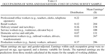
Such arguments are convincing only up to a point. Some of the jobs that youth were engaged in during the 1910s perhaps did require larger or special wardrobes, but many did not. Table 3 presents the occupational distribution of the working children in the sample as well as age- and gender-adjusted earnings by occupational category.⁴³

A substantial fraction of the sample worked in office or retail settings that would have required particular types of dress. But over half worked in factory, domestic service, or delivery or errand jobs that did not require more expensive wardrobes. Also, the rank ordering of earnings by occupation is not completely consistent with the notion that higher paying jobs required more expensive wardrobes. Office and retail establishment workers did have higher earnings than delivery and errand boys, but earnings were highest in production and transportation industry jobs.

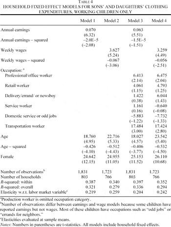
To examine this hypothesis more carefully, a number of robustness tests are considered. Table 4 presents the results from these tests. The first set re-estimates the wage and earnings models using only data on working children.⁴⁴

If the estimated effects of earnings and wages on clothing expenditures found in Table 2 were due only to the fact that labor market entry required larger wardrobes or more expensive forms of dress, than we would expect these effects to be attenuated when looking only at working children. This is not the case. Evaluated at the means of the sample, the elasticities of clothing expenditures with respect to earnings and wages were 0.22 and 0.26, respectively. Within the ranks of working children, clothing expenditures varied with income.

These results are still consistent, however, with the notion that certain types of jobs required special wardrobes and were also higher paying. To consider this version of the hypothesis, the earnings and wage models were re-estimated again using the working children sample, but now adding controls for occupational category. The addition of these controls has very little impact on the estimated effects of earnings and wages. These models do, however, provide some support for the hypothesis that different jobs had different clothing requirements. Even after controlling for wage or earnings, office and professional workers had higher clothing expenditures than production workers. Such workers would have had to project a particular image and so required more formal, and likely more expensive, attire. The data also indicate that workers in transportation jobs had higher clothing expenditures than workers in production jobs perhaps reflecting the outdoor nature of many transportation jobs and hence the need for heavier outerwear. But the bottom line that emerges from these models is that, even allowing that different types of jobs may have had different types of clothing requirements, expenditures on a child's clothing still depended on how much income she brought into the household.

DIFFERENCES IN BARGAINING POWER BY AGE AND GENDER

If interactions between parents and children took place within a bargaining framework, then we would expect that bargaining power would have varied with a child's age and gender as threat points, particularly in the form of exit options, varied with these characteristics. But as noted previously, having clothing expenditures as our only measure of private consumption makes it difficult to examine gender differences in bargaining power. All of the models presented in Tables 2 and 4 indicate that controlling for the age and labor market status of the child, households spent more on the clothing of daughters than on that of sons. This should not necessarily be interpreted as indicating that daughters had greater influence in household decisions. A more intuitive interpretation is that daughters preferred to have more of their private consumption in the form of clothes than did sons.

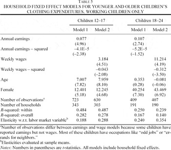
The clothing expenditure data do, however, allow us to explore differences in bargaining power by age. Needs and preferences for clothing likely did differ to some extent by age, but less so than by gender. The models in Tables 2 and 4 indicate that clothing expenditures did increase with a child's age. But a more sensitive test of increased bargaining power with age would be to determine if the effects of labor market status variables varied with age. If older children had more bargaining power because they had better opportunities to leave their parents' households, then they should have been better able to secure higher fractions of their earnings in the form of private consumption goods.

To test this hypothesis, the data for working children were divided into two samples: children ages 12 to 17 and children ages 18 to 24. As shown in Figure 1, while some youth younger than age 18 lived apart from their parents, it was not until age 18 that 20 percent or more did so. Eighteen was also, in most states during the period, the age at which young women could marry without their parents' consent.⁴⁵

Table 5 presents the wage and earnings models for the two age groups. The rewards of additional earnings were indeed greater for the older than for the younger group. The elasticities with respect to earnings and wages were 0.24 and 0.35 for sons and daughters ages 18 to 24 compared to 0.19 and 0.29 for sons and daughters ages 12 to 17. Also interesting is the difference in the effect of age across the two samples. Here, age is entered only linearly due to the smaller age ranges contained in each sample. For the sample of 12 to 17 year olds, clothing expenditures were increasing with age. But for the older sample, clothing expenditures did not vary with age. These patterns would seem to fit well with the notion that bargaining power varied with exit options. During early adolescence, opportunities to leave the parental household would have improved with each passing year. But after age 18, these opportunities changed very little from birthday to birthday.