INTRODUCTION
Farmers deal with field patterns that are increasingly split into areas far away from each other and with increased diversity. This is particularly the case for the farmers in the Massif Central (France), where a steady increase in the area used for cattle farming has been observed over the last decade. This contrasts with previous, more stable conditions (55 ha and 1·8 Annual Work Unit (AWU) in 2000 as against 69 ha and 1·8 AWU in 2007 on average for dairy cattle farms (Agreste 2008). Consequently, farmers have to manage fields with constraints that restrict their use. These constraints include: distance from farmstead, slope, small area and altitude. Distance and small area are determinant factors for grazing with dairy cows due to the necessity of going twice a day to the milking parlour (Morlon & Benoit Reference Morlon and Benoit1990; Brunschwig et al. Reference Brunschwig, Josien and Bernhard2006; Andrieu et al. Reference Andrieu, Josien and Duru2007). Slope is a major constraint when it comes to mechanization. This is associated with altitude and is a determinant of field use in mountain areas (Fleury et al. Reference Fleury, Dubeuf and Jeannin1996; Andrieu et al. Reference Andrieu, Josien and Duru2007). These constraints are often found on mountain fields and can reduce the season length and land use. Forage production and grazing are often modified by climatic uncertainties (Baumont et al. Reference Baumont, Deux, Farruggia and Jouven2008; Mosnier et al. Reference Mosnier, Agabriel, Lherm, van Itterson, Wolfe and van Laar2009). These constraints can increase costs and complicate the matching of fodder production adapted to animal requirements.
Field characteristics are key factors towards managing forage areas as they play an important role with regards to specific farm requirements. This is why research needs to focus on the development of new methods for the management of forage systems. Of special interest are models of livestock farm functioning that consider both temporal and spatial field uses. Martin et al. (Reference Martin, Hossard, Theau, Therond, Josien, Cruz, Rellier, Martin-Clouaire and Duru2009) present an expert discrimination tree based on 53 grassland uses, while Garcia-Launay et al. (Reference Garcia-Launay, Sibra, Molenat, Agabriel and Brunschwig2012) published a statistical discrimination tree for a cattle farm system based on 1586 field uses.
Land use classification can be thought of as a data mining issue. From this point of view, computational intelligence methods based on unsupervised learning are especially appropriate for understanding or extracting unknown information from different data sources. The purpose of unsupervised learning methods is to discover and cluster together similar groups from the input data. These data are usually represented as feature vectors in a highly dimensional space. Data belonging to one group are more similar than data belonging to different groups as defined by a similarity measure. This is also referred to as data clustering (Jain et al. Reference Jain, Murty and Flynn1999), being especially useful when information about the input data is unavailable or unknown.
The self-organizing map (SOM) is an unsupervised learning method that has been used widely for knowledge discovery, data mining, detection of inherent structures in highly dimensional data and mapping this data into a two-dimensional (2D) representation space (Kohonen Reference Kohonen1982). This mapping retains relationships within the input data and preserves its topology. The main advantage of this method is the visual understanding of data structures. Different visualization techniques have been used frequently to achieve a better understanding of the data (Vesanto Reference Vesanto1999). The SOM has several weaknesses: one is that the number and arrangement of the neurons has to be defined in advance; another is their inability to represent hierarchical relationships. The growing hierarchical self-organizing map (GHSOM) was proposed by Rauber et al. (Reference Rauber, Merkl and Dittenbach2002) to tackle both limitations. This neural network model has a hierarchical architecture divided into layers, where each layer is composed of different single SOMs with an adaptive architecture that is determined during the unsupervised learning process based on the input data.
In the present paper, the GHSOM model is used for the clustering and visualization of land usage data to achieve a hierarchical clustering. The understanding of this hierarchical clustering is improved by applying different visualization techniques to the maps at each layer. Knowledge of the management of forage production and grazing in grass-based livestock systems is needed to simulate their functioning and propose new practices. The remainder of the present paper is organized as follows. In the next section, a description of the GHSOM model and the training algorithm is provided. Then there follows a brief overview about land usage data and following that is a section presenting an experiment and its results consisting of the analysis and the visualization of land usage data with the GHSOM. The paper ends with a section presenting some conclusions.
HIERARCHICAL SELF-ORGANIZING MODEL
In the present paper, the GHSOM (Rauber et al. Reference Rauber, Merkl and Dittenbach2002) was used as a tool to perform hierarchical cluster analysis over land usage. The GHSOM can be considered as an extended version of the standard SOM (Kohonen Reference Kohonen1982), where a hierarchy of SOMs is constructed. The main purpose of SOMs is to map high-dimensional data into a 2D representation space, preserving the topology of the data. Thus, understanding of the data is gained by visualizing the resulting map. By using the GHSOM, hierarchical data understanding is also obtained and the size of the architecture does not need to be established in advance.
The GHSOM is an artificial neural network that consists of several growing SOMs (Fritzke Reference Fritzke1995) arranged in layers or levels, where the size of the architecture (number of neurons, maps and layers) is automatically determined during the unsupervised learning process, without having to decide this size beforehand. Initially, the GHSOM starts with a single SOM of 2×2 neurons, which is trained with the input data. After training, it can grow by inserting rows or columns of neurons until a certain level of detail in the representation of the data mapped onto the SOM is reached. Once the growing process has finished, the resulting neurons are examined to decide whether they are going to be expanded or not. The idea is to expand into a new map in the next layer of the hierarchy those neurons that represent the most heterogeneous clusters in order to provide a more detailed representation. Once the training process has finished, the final architecture of the GHSOM shows the clusters in which the data were mapped, where data belonging to one cluster are more similar than data belonging to different clusters. Moreover, this architecture reflects the inherent hierarchical relationships between the input data. An example of the architecture of a GHSOM is shown in Fig. 1.
Example of GHSOM architecture (colour version available online).

The adaptive growth process of the GHSOM is controlled by means of two parameters, τ 1 and τ 2. These two parameters are used to control the growth of the maps and the neural expansion into new maps of the GHSOM, respectively. The quantity of adaptation depends mainly on the quantization error (qe) of each neuron. The qe is a measure of the dissimilarity of the data mapped onto each neuron, where the higher the value of qe, the higher the heterogeneity of the data cluster. The qe of a neuron i is defined as follows:
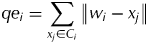 $$qe_i = \sum\limits_{x_j \in C_i} {\left\| {w_i - x_j} \right\|} $$
where C i is the set of input patterns mapped onto the neuron i, x j is the jth input pattern from C i, and w i is the weight vector of the neuron i.
Once a map m is trained, the possibility that the map can grow must be checked. The quantization error of each neuron (qe i) of the map m must be computed in order to compute the mean quantization error of the map (MQE m). If the MQE m is smaller than a certain fraction τ 1 of the qe of the corresponding parent neuron u in the upper layer, the map stops growing. This stopping criterion for the growth of the map is defined in Eqn (2). Otherwise, the map keeps growing to achieve a better level of representation of the data mapped onto the map, so the smaller the τ 1 parameter chosen the larger the map.
 $$MQE_m \lt \tau _1 \times qe_u $$
The growing of a map is done by inserting a row or a column of neurons between two neurons. These neurons correspond to the neuron with the highest quantization error e and its most dissimilar neighbour d. A row or a column is inserted if these two neurons belong to the same column or row, respectively. The index of the neuron d is computed according to Eqn (3), where ∧e is the set of neurons neighbouring e.
 $$d = \mathop {\arg \max} \limits_i (\left\| {w_e} \right. - \left. {w_i} \right\|),\quad w_i \in \wedge _e $$
Initially, the qe at layer 0 must be computed as given in Eqn (4), where w 0 represents the mean of the entire input data I.
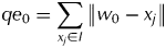 $$qe_0 = \sum\limits_{x_j \in I} {\left\| {w_0 - x_j} \right\|} $$
The initial quantization error (qe 0) measures the dissimilarity of all input data and it is used for the neural expansion process of the GHSOM together with the τ 2 parameter, as given in the stopping criterion of the neural expansion Eqn (5). In this stopping criterion, the quantization error of a neuron i (qe i) must be smaller than a fraction (τ 2) of the initial quantization error (qe 0) to be a leaf neuron (non-expanded neuron). Otherwise, the neuron is expanded into a new map at the next level of the hierarchy, so the smaller the τ 2 parameter, the deeper the hierarchy.
 $$qe_i \lt \tau _2 \times qe_0 $$
When a new map is created from an expanded neuron, a coherent initialization of the weight vectors of the neuron is used as proposed by Dittenbach et al. (Reference Dittenbach, Rauber, Merkl, Allinson, Yin, Allinson and Slack2001). This initialization provides a global orientation of the individual maps in the various layers of the hierarchy. Thus, the weight vectors of neurons mirror the orientation of the weight vectors of the neighbour neurons of their parents. The proposed initialization computes the mean of the parent and its neighbours in their respective directions.
A newly created map from its parent neuron is trained as a single SOM. During the training, the set of input patterns are those that were mapped onto the parent neuron. In each iteration t, an input pattern is randomly selected from this data subset. The winning neuron of the map is the neuron with the smallest Euclidian distance to the input pattern, whose index r is defined as:
 $$r(t) = \arg \mathop {\min} \limits_i (\left\| {x(t) - w_i (t)} \right\|)$$
The winner's height vector is updated according to Eqn (7). Here, the amount of adaptation is guided by a learning rate α, decreasing in time. In addition to the winner, the winner's neighbours are updated depending on a Gaussian neighbourhood function h i and their distances to the winning neuron. This neighbourhood function, Eqn (8), reduces its neighbourhood kernel δ during training, being  $\left\| {r{}_c - r_i} \right\|^2 $ the distance between neurons c and i within the output space, with r i representing the 2D coordinates of the neuron i within the grid.
 $$w_i (t + 1) = w_i (t) + \alpha (t)h_i (t)\left[ {x(t) - w_i (t)} \right]$$
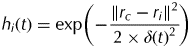 $$h_i (t) = \exp \left( { - \displaystyle{{\left\| {r_c - r_i} \right\|^2} \over {2 \times \delta (t)^2}}} \right)$$
LAND USAGE DATA
The dataset was organized based on: geographical characteristics, practices and season of forage production, usage (cutting and grazing) and forage supply during grazing.
Description of the traditional salers livestock system
The Traditional Salers Livestock System is located in the Massif Central, France, mainly in the departments of Cantal and Puy-de-Dôme. One mountain breed of cows exploited in these departments is the hardy Salers, which is a dual purpose breed (milk and store production). These cows produce milk concurrently for milking and suckler calves. The calves initiate the milking process. Suckling follows the milking activity. This traditional dual milking production model has been observed in different mountain areas (Teissier Reference Teissier1979).
The survey
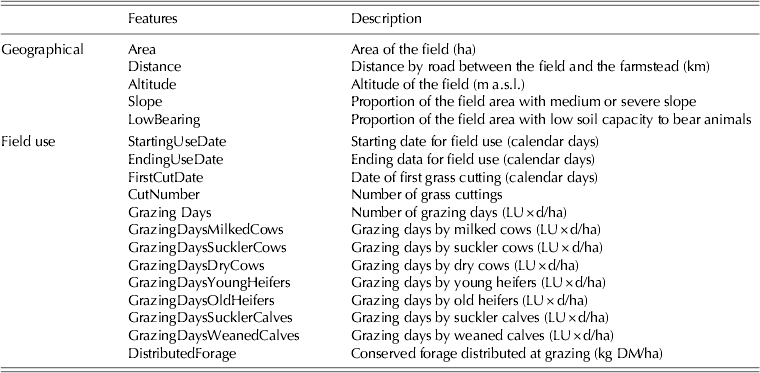
A survey in the Salers farms population was done in order to get a representative sample (Garcia-Launay et al. Reference Garcia-Launay, Sibra, Molenat, Agabriel and Brunschwig2012). These 72 farms are characterized by medium values for: agricultural area (78 ha), number of cows (43) and low milk quotas (69 000 l/year) compared with the average values observed in France (40 cows with 254 000 litres of milk collected per farm and per year) (Institut de l'Elevage 2008). Milking duration per year varies from a seasonal period of 135 days to all year long. Altitude ranges from 430 to 1400 m a.s.l., which is characteristic of these mountainous areas. The farm systems are based entirely on permanent grasslands with a grazing period duration of 7·5 months on average. Within the sample, 43 farms managed a dual-purpose herd and 29 farms managed both a dual-purpose and a suckler herd. Data were collected for each farmer in 2005 (Agabriel et al. Reference Agabriel, Sibra, Journal and Coulon2005). The data concerned the farming system with a focus on animal production and forage management. The information obtained was about herd composition, animal grouping, feeding supply (forage and concentrate) per group throughout the year and also about the total quantities of conserved forage produced and bought. The field was considered as the smallest functional and spatial unit (Thenail & Baudry Reference Thenail and Baudry2004) with homogeneous land use in 2005. Farmers were asked to characterize each field geographically (n=1586) based on: area, distance to farmstead, slope, altitude and soil capacity (Table 1). Aerial photographs were used to validate the values obtained. The farmers’ own perception of the areas/fields with low bearing capacity and with medium or severe slope was also used for validation purposes. It was considered that the farmers’ perception had a higher correlation with the grassland use than measured variables.
Geographical and field use features
A detailed cutting and grazing schedule was drawn up for each field (Table 1) and reports produced, including: cutting dates, type of conserved forage harvested, entrance and exit dates of animal groups, and quantity of forage supplied at grazing. Fields that were cropped (n=23), used by other farmers (n=28) or abandoned (n=35) were excluded from the present study.
RESULTS
In order to demonstrate the application of GHSOM in the field of land use classification, several experiments and results are described in this section. These experiments consist of the analysis and data visualization of geographical and field use characteristics and cutting and/or grazing practices in three general groups of fields: cut only, cut and grazed and grazed only fields. Land use analysis and subsequent visualization of the resulting data was based on GHSOM models. The resulting data visualizations are useful to help characterize the types of grassland use in a mountain cattle farm system and to link them to the geographical characteristics of the fields. This provides a conceptual model of grassland use that can be easily adapted to counselling and modelling needs.
Data preparation
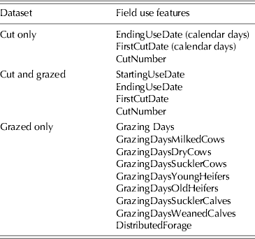
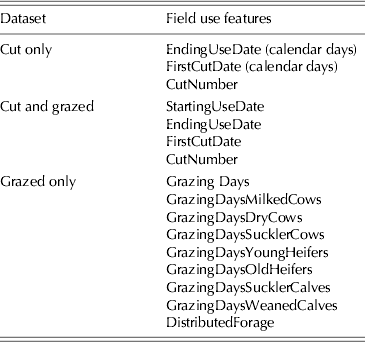
For each of the three datasets, both the field use and the geographical features were taken into account for the cluster analysis. A description of the field use and geographical features utilized in these datasets is given in Table 1. The five geographical features are present in the three datasets. These are: area, distance, altitude, proportion of area with medium or severe slope and with low bearing. Some datasets contained missing values, which were removed from the datasets. Since the aim is to cluster the data samples, the class labels were not included. The first dataset corresponding to cut only fields contained a total of 112 samples and eight features, with three field use features and five geographical features. The second dataset (cut and grazed) had a total of 660 samples with nine features (four field use and five geographical). Finally, the third dataset (grazed only) contained 746 samples with 14 features (nine from field use and five geographical). The field use features present in each dataset are shown in Table 2.
Field use features per dataset
Data visualization
The three datasets were used to train the GHSOM model in order to build a hierarchical clustering model of the data. The τ 1 and τ 2 parameters were set to 0·1, since this achieves a small architecture of two layers that can be easily analysed and understood. Ten runs were performed for each dataset, generating ten architectures for each one. All the architectures obtained by training with the same dataset were similar to each other. However, they were not exactly the same since the input samples were presented randomly to the neural network. Therefore, the architecture that achieved the best level of clustering, considered to be the one with the minimum sum of qe of the hierarchical model (see previously), was selected in order to analyse the results of each dataset.
For the sake of simplicity, only the visualizations corresponding to the first dataset are shown in the present paper. Thus, the hierarchical 3D architecture and its projection in a 2D map for the selected model from the first dataset are shown in Figs 2 and 3, respectively. In Fig. 2, the architecture has two layers and three maps in the second layer. All the obtained architectures for the three selected models have two layers with three or four maps in the second layer, so the analysis performed in the present paper for the first dataset is valid for the two remaining datasets. Each sphere represents a neuron. Numbers were assigned to each neuron in order to identify them. The expanded neurons are represented with darker shades and without horizontal lines. An arrow going out from the neuron indicates the map into which it was expanded. The 2D projections of these hierarchies can help in visualizing the neural subdivision at a glance. In Fig. 3, each square represents either a neuron (if it contains a circle in its centre) or a map (if it is subdivided into more squares). The smaller the size of the square the deeper the layer it belongs to (the biggest square is the map at layer zero). It can be seen in these plots how for the first architecture, neurons 3, 5 and 6 were expanded into three maps of 3×2, 4×2 and 3×3 neurons, respectively. These two representations of the hierarchical architecture provide a better understanding of the resulting clustering for each dataset corresponding to different cutting and/or grazing practices.
Three-dimensional architectures for the cut only dataset. Each sphere represents a neuron and identification numbers were assigned to each neuron. The expanded neurons are represented with darker shades and without horizontal lines (colour version available online).
Two-dimensional projections of the hierarchical architectures for the cut only dataset. Each square represents a neuron or a map, where the smaller the size of the square, the deeper the level of the hierarchy of the neuron or map. Thus, the biggest square represents the neuron at layer-0 map and the smallest one a neuron at layer 2. Numbers were assigned to each neuron (colour version available online).
By observing the obtained architectures, the relationships and arrangement among clusters can be analysed, although information about the input data mapped into the clusters is not reflected. In order to show the relationship between the input data and the clusters, more visualization techniques are used. One of these techniques is to plot the input data hits, which shows the number of samples mapped onto each cluster of the architecture. The distribution of samples into clusters for the obtained hierarchy corresponding to the first dataset is given in Fig. 4. The relative number of samples for each neuron is also shown by means of the size of a coloured patch. Note that those neurons with larger numbers of mapped data are expanded. In this plot, it can be seen that for the cut only field, from the 112 samples initially mapped, 25, 30 and 35 were expanded into three new maps in the second layer. In the maps from the second layer of the architecture, neurons with no samples associated can be detected. These neurons are considered ‘dead’ and do not provide any information about the clustering performed. Thus, they can be ignored from now on.
Input data hits for the architecture corresponding to the cut only dataset. Each square represents a neuron with its number of samples associated and also the relative number of samples by means of the size of a coloured patch. The neurons with a larger number of samples are the ones that have been expanded (indicated with an arrow). Neurons without any sample associated are considered dead neurons (colour version available online).
Another useful visualization technique to obtain more information about the data mapped into the clusters is the plot of the component planes. This shows the distribution of the feature values in order to see the spread of data from each feature (or component) in all map neurons. By comparing the corresponding component planes for each feature, possible correlations among features can be discovered. The component planes of the maps corresponding to the first group of field are given in Fig. 5. In the plots, there is a component plane per feature, where larger weights (higher values of a feature) are represented by darker shades. A colour legend shows the values of the component planes normalized between 0 and 1. Dead neurons are coloured in grey and must be ignored in the analysis since they do not represent any data cluster. By observing these plots, no correlations are detected among features, indicating that the features were selected properly. In Fig. 6, a detail of the component planes for the ‘FirstCutDate’ feature is given, where the hierarchical relations of the component planes can be better perceived.
Component planes for the cut only dataset: (a) layer-1 map, (b) layer-2 first map, (c) layer-2 second map and (d) layer-2 third map. Larger weights are represented by darker shades. A colour legend is shown, where the values of the component planes are normalized between 0 and 1. Dead neurons are coloured in grey (colour version available online).
Component planes for the ‘FirstCutDate’ feature corresponding to the architecture of the cut only dataset. Larger weights are represented by darker shades. A colour legend is shown, where the values of the component planes are normalized between 0 and 1. Dead neurons are coloured in grey (colour version available online).
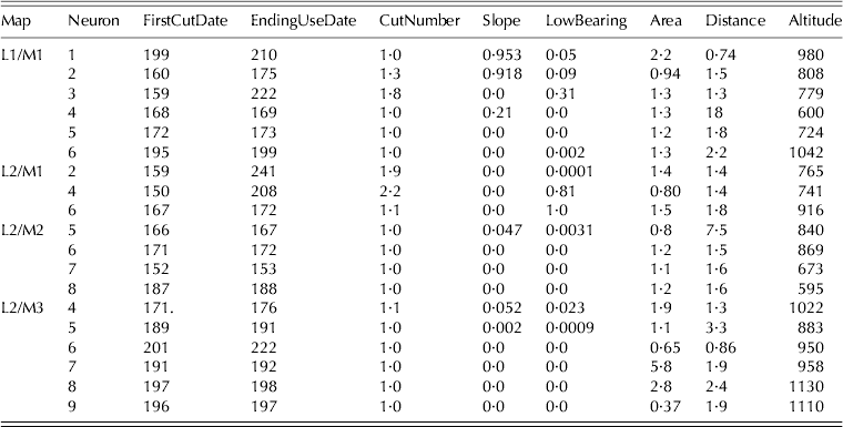
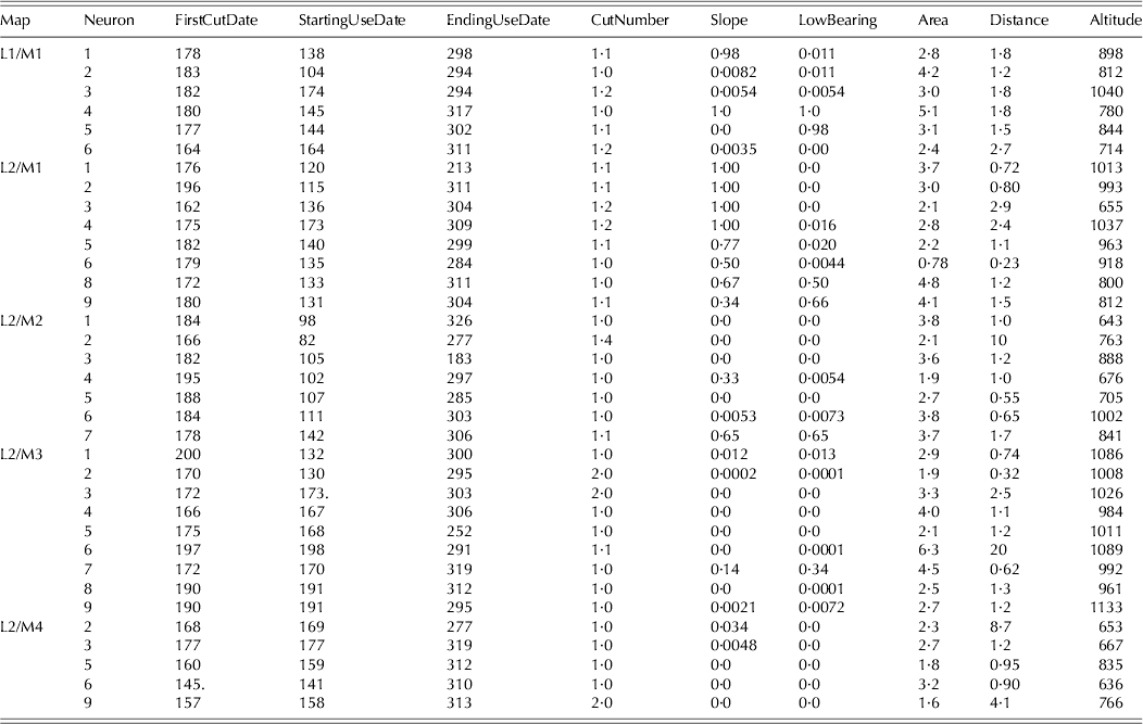
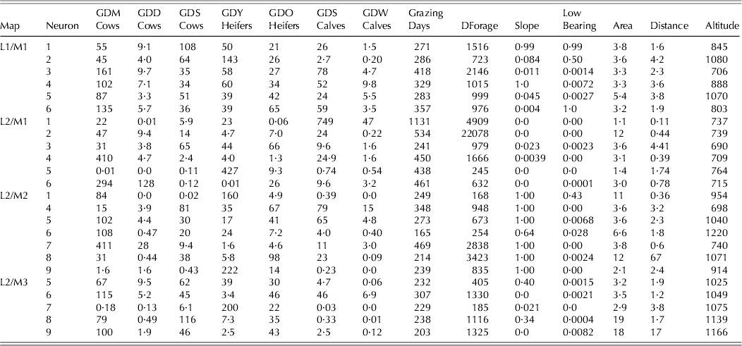
Apart from detecting possible correlations among features, more information can be extracted from these plots. This information is summarized in Tables 3–5 for the cut only, cut and grazed and grazed only field groups, respectively. Here, it can be seen that the values representing all the data mapped onto each cluster in each field group.
Considering the cut only fields (Table 3), the L2/M3 map could be characterized as fields with late cut and relatively elevated altitude (cf. Neuron 9), the L2/M2 map as fields with early cut (cf. Neuron 5), and the L2/M1 map as fields with two cuts and/or low bearing (cf. Neuron 4), while L1/M1 map appears to be more heterogeneous.
Values of the component planes from the cut only field architecture
For the cut and grazed fields (Table 4), the L2/M4 map could be characterized as fields with long periods of use, early first cut and late ending date, and situated at low altitude (cf. Neuron 9), the L2/M3 map as fields with late first cut, medium usage end date and located at elevated altitude (cf. Neuron 6), the L2/M2 map as fields with a longer period of use, early grazing before a first cut, a medium ending date, and situated at low altitude (cf. Neuron 5), the L2/M1 map as fields with grazing before a first cut, medium ending date, high proportion of area with medium or severe slope and situated at medium altitude (Neuron 5) and L1/M1 map as fields with grazing before an early first cut, a late ending date, with slope or low bearing, a relatively large area and long distance from farmstead and medium altitude (cf. Neuron 4).
Values of the component planes from the cut and grazed field architecture
For the grazed only fields (Table 5), the maps were characterized as follows: L2/M3 map as fields used by milking cows and suck-ling cows, medium forage distribution and grazing days and situated at elevated altitude (cf. Neuron 8), L2/M2 map as fields grazed by milking cows, heterogeneous grazing days and forage distribution, with high proportion of area with medium or severe slope and relatively large area (cf. Neuron 5), L2/M1 map mainly grazed by milking cows, with high grazing days and forage distribution, situated at small distance from farm-stead and low altitude (cf. Neuron 4), and L1/M1 map as fields more grazed by suckling cows and heifers, with high grazing days and forage distribution, and situated at long distance from farmstead and medium altitude (cf. Neuron 2).
Values of the component planes from the grazed only field architecture
CONCLUSIONS
Geographical characteristics are key discriminators of grassland use. A hierarchical visualization of land usage data was provided using a GHSOM neural network. The GHSOM is composed of several independent growing SOMs, arranged in a hierarchical architecture, that are automatically established during the unsupervised learning process. As a consequence, this hierarchical architecture provides a more flexible adaptation to input data than a single SOM and a better capture of the relationships among them. Therefore, the improvement in data modelling provides a better visualization and understanding of the input data. By using the GHSOM for land usage data, the provided hierarchy of SOMs can be analysed to extract relevant information about the mapped data. This may aid agronomists and farmers to better understand hidden relationships in the datasets.
In the present paper, a dataset obtained by capturing data from 1586 was utilized to train the GHSOM algorithm. Different visualization techniques were used to represent different maps. After considering all the data plots together with the hierarchical architecture, a better insight of the data was achieved and several clusters could be identified along the hierarchy. The proposed hierarchical model of grassland use shows that a combination of geographical characteristics may be associated with several types of grassland use. The use of these fields may be adapted according to weather conditions and herd requirements during the grazing season. The map obtained highlighted groups that could be characterized by types of field use related to some geographical characteristics, while the neurons enabled a better characterization of this relationship. This way to classify field uses could be of interest as input in a farm simulator to specify the possible uses of fields associated to their geographical characteristics. This is particularly interesting in case of in silico experiment or in case of complete reorganization of grazing and forage system or of farming systems. Further investigation will consider the influence of field pattern characteristics on these relationships.