1. Introduction
In recent years, the global phenomenon of climate change has become increasingly evident, with rising temperatures posing significant challenges to various aspects of human life and economic activity. Studies have found that climate change in the long run and its short-run counterpart – that is, weather shocks – adversely affect aggregate output, agriculture, labour productivity, health, energy, and even conflict and crime, among other outcomes (Dell et al., Reference Dell, Jones and Olken2014). The negative effect of weather shocks also disproportionately affects less developed countries as they have weaker institutions and high reliance on agriculture (Paglialunga et al., Reference Paglialunga, Coveri and Zanfei2022), which in turn exacerbates the problem of inequality (Palagi et al., Reference Palagi, Coronese, Lamperti and Roventini2022), both across and within countries. Studies have also found that the effects of temperature rise become more visible after reaching certain thresholds (Dell et al., Reference Dell, Jones and Olken2014), implying that countries with already-warm climates will pay the highest price of global warming. However, evidence on the effects of temperature shocks on micro and small enterprises remains limited despite their critical role in many economies, particularly in developing countries.
This study examines the impact of temperature on labour productivity in micro and small enterprises in Indonesia – an expansive archipelago with a complex socio-economic landscape that faces heightened vulnerability to rising temperatures due to its equatorial position. As temperatures continue to rise, there is a pressing need to understand the implications for productivity, livelihoods and overall economic well-being, especially within the informal sector, where a substantial portion of the population is engaged. As in other developing countries, Indonesia’s micro and small enterprises are mostly informal household-based businesses and serve as the primary livelihood source for many, particularly the poor. Unlike larger enterprises, they also lack the resources to cope with rising temperatures.
In Indonesia, micro, small and medium enterprises (MSMEs) form the backbone of the economy, accounting for 99 per cent of all business units, contributing 60.5 per cent to GDP and employing nearly 97 per cent of the workforce (Coordinating Ministry of Economic Affairs, 2024). Strikingly, around 85 per cent of these enterprises are operated from within the household (Kadin Indonesia, 2023), underscoring the central role of household-based enterprises in shaping livelihoods and economic resilience. Despite their scale and significance, this segment remains understudied, as prior research has largely focused on MSMEs more broadly without disentangling the unique dynamics of enterprises embedded in the household setting. Studying household-based enterprises is therefore essential, not only because they constitute the most common form of business in Indonesia, but also because they reflect the intersection of family, livelihood and enterprise, operating under distinct constraints and vulnerabilities compared to more formalized firms.
We use data from the non-farm business module in the Indonesian Family Life Survey (IFLS) merged with gridded climate data – particularly temperature and precipitation. The combination of the two datasets presents a unique opportunity to explore how temperature variations affect labour productivity in micro and small enterprises. Particularly, as a comprehensive household survey covering a wide range of socio-economic aspects of household-based enterprises, the IFLS offers rich information to examine the impact of temperature on productivity outcomes – measured by annual earnings per labour – and identify the transmission explaining the impact mechanism. The merged data also enables us to explore the possible heterogeneous effects across economic sectors and other dimensions.
In estimating the impact of temperature rise on productivity, our estimation strategy relies on plausibly exogenous temporal temperature variations within each geographic area. In addition to some relevant covariates, we also control for two fixed effects (FE): subdistricts and year-month of survey. The subdistrict FE handles potential correlation between temperature – and precipitation level – with unique (unobserved time-invariant) subdistrict heterogeneity that might also explain the productivity. The year-month of survey and temperature measurement FE capture nationwide temperature movement that might coincide with movement in productivity. We also control household-level characteristics that might correlate with productivity. After all of these, we argue that the estimated temperature parameter reflects the unbiased impact of temperature on workers’ productivity in household-based enterprises.
Our findings indicate that a 1°C increase in the 12-month average temperature deviation reduces revenue by 13–14 per cent and revenue per worker by 20–21 per cent. We further find that the effect of temperature rise on productivity is nonlinear, following an inverted U-shaped relationship, with productivity peaking at around 25–26°C. The effects are also heterogeneous, disproportionately affecting businesses that are located in already warmer areas; smaller businesses; and those in sectors demanding intensive labour, such as construction and manufacturing. The findings highlight the significant impact of climate-induced temperature changes on labour productivity in vulnerable economic sectors, emphasizing the need for targeted policies to enhance climate resilience in Indonesia’s household-based enterprises.
Our study contributes to at least two distinct strands of literature. Firstly, it engages with the very limited body of work on the effects of weather shocks on micro and small enterprises, an area where many aspects remain underexplored. Among the few existing studies are Churchill et al. (Reference Churchill, Munyanyi, Trinh and Wiklund2024), who examine the impact of extreme weather on self-employment in Australia, and Francisco et al. (Reference Francisco, Lau and Mendoza2014), who analyse small and medium enterprises (SMEs) resilience to flooding in the Philippines. In summary, prior research shows that weather shocks significantly reduce the prevalence and resilience of small- and medium-scale enterprises and self-employment.
Secondly, our study strengthens the evidence on the adverse impacts of climate change and weather shocks in the Indonesian context. For instance, Levine and Yang (Reference Levine and Yang2014) investigate the effects of rainfall shocks, Caruso et al. (Reference Caruso, Petrarca and Ricciuti2016) assess the impact of temperature on agricultural production and Chaijaroen (Reference Chaijaroen2019) explores how coral bleaching induced by rising sea temperatures affects fishery household incomes. More recently, Xie (Reference Xie2024) examines how temperature shocks influence the dynamics and input bundle choices of medium and large firms in Indonesia. Collectively, these studies found that climate shocks, specifically rainfall volatility, temperature shocks and coral bleaching, significantly disrupt output across the agricultural, fishery and manufacturing sectors.
However, there remains a notable lack of emphasis on the specific vulnerabilities and adaptive capacities of household-based SMEs in the Indonesian context. Extending this literature, our work provides new micro-level evidence from home-based firms and shows variation in the degree of susceptibility to temperature shocks across locations. In particular, our results show that enterprises located in areas with higher temperatures experience substantially larger productivity losses. It adds a spatially nuanced perspective to the micro-enterprise and informal-sector climate literature.
The paper is organized as follows. Section 2 surveys the previous studies that link climate with various measures of well-being and productivity. Section 3 provides a discussion on both data sources, the IFLS and the climate data. The empirical strategy is outlined in Section 4, followed by a discussion of the results in Section 5. Finally, Section 6 provides some conclusions and implications.
2. Literature review
The connection between climate change and productivity has become a crucial focus in research as rising global temperatures bring new challenges. Climate change is raising the frequency and intensity of extreme climate events, such as heatwaves, droughts and floods. This poses substantial risks for businesses, industries and economies worldwide. A study by Hübler et al. (Reference Hübler, Klepper and Peterson2008) also indicates that rising temperatures impair work performance, potentially leading to a significant GDP loss. To understand where these losses come from, recent works trace micro-level pathways from temperature shock to labour productivity.
The first pathway is direct physiological strain. Worker productivity declines as heat exposure rises (Dasgupta et al., Reference Dasgupta, Maanen, Gosling, Piontek, Otto and Schleußner2021). High-frequency factory data from India show substantial effects: on hot days, each additional degree lowers output by about 4–9 per cent and increases absenteeism (Somanathan et al., Reference Somanathan, Somanathan, Sudarshan and Tewari2021). Heat also compromises safety, with extreme ambient temperatures associated with more occupational injuries and lost workdays (Martínez-Solanas et al., Reference Martínez-Solanas, López-Ruiz, Wellenius, Gasparrini, Sunyer, Benavides and Basagaña2018). These findings are consistent with a broad literature linking heat to pervasive productivity losses across settings and regions (Kjellström et al., Reference Kjellström, Kovats, Lloyd, Holt and Tol2009; Dunne et al., Reference Dunne, Stouffer and John2013; Dell et al., Reference Dell, Jones and Olken2014).
The second pathway operates through cognition and mental health. Elevated temperatures impair decision-making: hyperthermia disrupts brain connectivity (Sun et al., Reference Sun, Qian, Jiang, Li, Li, Li and Liu2013), slows reactions and reduces accuracy (Gaoua et al., Reference Gaoua, Racinais, Grantham and Massioui2010), impairs rational choice and patience (Escobar Carias et al., Reference Escobar Carias, Johnston, Knott and Sweeney2024) and weakens judgment in high-stakes tasks (Thompson et al., Reference Thompson, Ferrie, Pearson, Highlands and Matthews2024). Afridi et al. (Reference Afridi, Mahajan and Sangwan2022) also find that droughts exert long-lasting impacts on well-being in agriculture, with women disproportionately affected. Taken together, these cognitive and psychological channels compound the direct physiological effects, lowering effective labour supply and elevating error risk.
These mechanisms do not hit all workers equally. Exposure varies with tasks and baseline climate, producing pronounced sectoral and spatial heterogeneity. In crop production, heat stress depresses labour productivity with implications for global food security (Orlov et al., Reference Orlov, Daloz, Sillmann, Thiery, Douzal, Lejeune and Schleussner2021). Outdoor, labour-intensive sectors such as construction face a slower work pace, more breaks and higher health risks under extreme heat. Because many tropical regions begin from higher baseline temperatures, the same shock generates larger productivity losses there, which points to the need for region-specific adaptation (Knittel et al., Reference Knittel, Jury, Bednar-Friedl, Bachner and Steiner2020; Orlov et al., Reference Orlov, Daloz, Sillmann, Thiery, Douzal, Lejeune and Schleussner2021).
At the macro level, diminished labour productivity reduces output, raises costs and erodes competitiveness – pressures that are especially acute in labour-intensive developing economies (Fankhauser and McDermott, Reference Fankhauser and McDermott2016). Yet losses are not inevitable: stronger social support and adaptive capacity cushion impacts (Knittel et al., Reference Knittel, Jury, Bednar-Friedl, Bachner and Steiner2020), while practical workplace adaptations – climate control, shifting hours to cooler periods and hydration/rest protocols – help sustain performance (Zhu et al., Reference Zhu, Wang, Zhang and Wang2021). In sum, the evidence converges on a coherent picture: climate shocks, and heat in particular, depress labour through physiological, psychological and cognitive channels, with uneven burdens across sectors and regions and economy-wide consequences that well-designed adaptation can partially offset.
While much of the literature focuses on workers, large firms and macroeconomic impacts, evidence on small businesses remains limited. Notable exceptions include Churchill et al. (Reference Churchill, Munyanyi, Trinh and Wiklund2024), who study the impact of extreme weather on self-employment in Australia, and Francisco et al. (Reference Francisco, Lau and Mendoza2014), who assess SME resilience to flooding. Tarsia (Reference Tarsia2024) extends this by analysing the effect of temperature shocks on firm performance across Europe. Building on this, our study contributes new evidence on how climate change affects productivity in household businesses within a developing economy. Specifically, we focus on micro and small household-based enterprises in Indonesia, most of which operate informally and face distinct challenges in adapting to climate shocks. Unlike Xie (Reference Xie2024), who analyses medium and large firms in Indonesia, our study targets small, often home-based businesses that form a substantial part of employment in emerging economies. While Somanathan et al. (Reference Somanathan, Somanathan, Sudarshan and Tewari2021) use manufacturing data from India to quantify heat-related productivity losses, our research offers insights from Indonesia’s archipelagic context, where businesses are geographically dispersed, resource-constrained and embedded in diverse microclimates.
Indonesia is a particularly relevant case: as the world’s fourth most populous country and an upper-middle-income economy, it has a high concentration of household-based firms that are vital to livelihoods yet highly vulnerable to environmental stressors (Dell et al., Reference Dell, Jones and Olken2014; Paglialunga et al., Reference Paglialunga, Coveri and Zanfei2022). Its equatorial climate, vast geography and socio-economic diversity make it a critical setting for understanding how temperature shocks affect small-scale enterprise productivity. This context is essential for designing targeted climate adaptation strategies in tropical developing countries, where informality and limited adaptive capacity can intensify the adverse effects of rising temperatures.
3. Data
3.1. Household businesses
The main data of this study comes from the IFLS, an extensive household-level longitudinal survey that measures a rich set of information at individual, household and community levels. The survey was first conducted in 1993, using a sampling frame representing nearly 83 per cent of the Indonesian population. The first round was followed by four consecutive rounds in 1997, 2000, 2007 and 2014 (Strauss et al., Reference Strauss, Beegle, Sikoki, Dwiyanto, Herawati and Witoelar2004, Reference Strauss, Witoelar, Sikoki and Wattie2009, Reference Strauss, Witoelar and Sikoki2016). The actual fieldwork for each round takes place within a 1-year span, thus creating even bigger temporal variation. In the case of splitting households (e.g., due to marriage), IFLS followed both the original and the newly created households, explaining the growing household sample size.
IFLS has a module on household businesses aimed at all households running any non-agricultural business currently in operation or which had been shut down in the last 12 months. This module collects essential information, including the year of establishment, revenue and cost, physical capital, number of workers and business sector. As time progressed, IFLS expanded the questions in every new survey round while keeping the existing items. Older rounds of IFLS tend to have more limited information than its newer rounds. For this reason, we restrict our sample to only containing the last three rounds of IFLS, allowing us to construct our outcomes and to include other variables of interest. When the sampled households operate more than one business, the survey asked the households to identify the main and the secondary businesses, and collect the information from all businesses run by the households. More recent IFLS rounds record more businesses owned by households. To maximize statistical power, we include all the businesses recorded in the dataset in our sample.
The main outcomes of this study are revenue and revenue per worker, which serve as a proxy for productivity. The revenue variable is constructed from self-reported questions asked to the household member who has knowledge of the daily operation of the business. It is recorded for the last 12 months prior to the survey in an aggregate figure. For the firm’s number of workers, the survey includes both paid and unpaid workers employed by the firm at the time the survey was conducted. In the case of own-account workers, we purposively add ‘1’ to the number of workers to account for the owner herself. This procedure also eases the conversion to a natural logarithm.
One potential concern is employment seasonality. In our case, this may be a concern since the timing of the interviews was different across households, which then may determine the number of workers employed by the business in that particular interview month. Indeed, in Appendix Table A1, we show that employment tends to jump at the end of year. This motivates us to include a temporal FE empirical specification, which is discussed in the next section. From the survey data, we also generate some control variables, including the current value of physical capital (total value of lands, buildings, vehicles and equipment), age of business, sector and business location (home-based or outside home).
Table 1 provides summary statistics for all variables in the study: the upper panel displays the summary statistics for climate-related variables, while the lower one shows those of household business variables. Of the more than 12,600 household businesses in the sample, approximately 4,700 are from IFLS3, 4,300 from IFLS4 and 3,600 from IFLS5. The smaller number in the last round is due to the limitation of the recorded number of businesses per household to a maximum of two. The sample is dominated by microenterprises with an average number of workers of only slightly higher than two, even after counting the owner as the business’s worker. Almost half of the businesses are fully or partially home-based, mostly from the trade and restaurant sector. Despite being specifically aimed at non-agricultural businesses, some of them are nonetheless captured in the dataset. The average age of businesses is considerably high at around 10 years.
Summary statistics

3.2. Climate data
Our main treatment variable in this study is temperature, obtained from the Global Historical Climatology Network version 2 and the Climate Anomaly Monitoring System (GHCN CAMS) gridded data (Fan and van den Dool, Reference Fan and van den Dool2008). GHCN CAMS measures the average monthly land surface air temperature at a spatial resolution of 0.5 by 0.5 degrees. It also provides long-term mean (LTM) temperature for each calendar month, which we utilize to calculate temperature deviation from the ‘normal’ condition. We use this temperature deviation in our main specification as a measure of temperature shocks. In addition to temperature, we also use monthly precipitation data obtained from the Global Precipitation Climatology Centre (GPCC) (Rustemeier et al., Reference Rustemeier, Hänsel, Finger, Schneider and Ziese2022) as a control variable. GPCC measures total monthly precipitation at a spatial resolution of 0.25 by 0.25 degrees.Footnote 1
We then merge the climatic gridded data with household-based firms. Particularly, we match each subdistrict’s centroid in IFLSFootnote 2 with the nearest non-missing climatic grid. In total, 284 IFLS subdistricts are matched to 114 grids, providing enough variation for temperature shock effect identification. Appendix Figure A1 shows the distribution of the subdistricts included in the sample, along with the matched temperature grids. The outcome variable, revenue per worker, is measured as a total annual value for the last 12 months preceding the survey. Because the climatic data comes in monthly frequency, we match it with household data by first calculating the corresponding 12-month average.
Appendix Figure A2 shows the summary of monthly temperature data for grids that are matched with the IFLS sample for the entire time span between 2000 and 2016. Appendix Table A2 further shows the monthly mean and median of temperature level and temperature deviation. Appendix Figure A2 shows a clear annual seasonal pattern. In the matched grids, annual temperature has two peaks, in April and October (with a median temperature of 27.2°C and 27.4°C, respectively) and has two troughs, in February and July (with a median temperature of 26.4°C and 26.1°C, respectively). However, after subtracting the calendar month LTM from the raw temperature data, the temperature deviation is apparently stochastic. Appendix Table A2 shows that the temperature tends to be most volatile in January, with a median deviation of around 0.35°C and the least volatile in August, with a median deviation of around 0.15°C. The seasonality of temperature patterns might coincide with the seasonality of economic environment patterns, which might bias the temperature–productivity relationship. This motivates us later to include year-month FE in our regression framework. In addition to temperature, the precipitation data also exhibit a clear seasonal pattern (see Appendix Figure A4), which disappears after removing the LTM.
The distribution of temperature variables for the matched grids and periods is shown in Appendix Figure A3. Panel A shows the 12-month average of temperature. The distribution is left-skewed, reflecting the distribution of population and settlements, which mostly reside in lower altitudes. Panel B, on the other hand, shows the 12-month average deviation from LTMs. The distribution is more symmetrical due to the more stochastic nature of temperature shocks. Relatedly, Appendix Figure A5 presents the distribution of precipitation variables for the matched grids and periods, which, in contrast to temperature, is slightly right-skewed.
4. Empirical strategy
4.1. Identification strategy
Our empirical strategy to establish the causal effect of temperature shock on productivity relies on plausibly exogenous temporal variations of temperature (and other weather-related variables) within each geographic area. In this study, we define the geographic area as a subdistrict (kecamatan), the lowest administrative division identifiable from the survey data, which is publicly available. The use of a lower-level administrative division, village, is not needed as the resolution of gridded temperature data is wide enough to cover several subdistricts.Footnote 3
Specifically, our empirical model is as follows:
 \begin{equation}{y_{ijt}} = {\beta _1}tem{p_{jt}} + {\beta _2}preci{p_{jt}} + \,{{\boldsymbol{\gamma }}^{\boldsymbol{'}}}{{\boldsymbol{x}}_{{\boldsymbol{ijt}}}} + {\phi _j} + {\tau _t} + {\varepsilon _{ijt}},\end{equation}
where y is our outcome variable (log revenue and log revenue per worker) of household business i residing in subdistrict j at time t (survey month). Our treatment variable of interest is temp, which is the 12-month average surface temperature deviation preceding the surveys that were conducted in year-month t. Temperature deviation is defined as the deviation from the monthly LTM. We also include precip, which is a 12-month average of monthly precipitation, as another measure of weather shock. This inclusion of a precipitation variable causes the temperature coefficient to reflect the temperature shock’s effect on productivity net of its effect through the rainfall change channel. This inclusion is a standard practice in the temperature effect literature (see, e.g., Dell et al., Reference Dell, Jones and Olken2014; Somanathan et al., Reference Somanathan, Somanathan, Sudarshan and Tewari2021; Tarsia, Reference Tarsia2024; Xie, Reference Xie2024). Vector x contains a set of household business characteristics, which are not the transmission channels through which temperature shock affects the outcomes.
In the model, we also control for  ${\phi _j}$ and
 ${\tau _t}$, which respectively represent the subdistrict FE and year-month FE. The subdistrict FE addresses the potential endogeneity of temperature caused by the heterogeneity of climate across regions. Furthermore, adding year-month FE to the model captures nationwide temperature movements that may coincide with changes in productivity. The inclusion of these FE remains necessary even after netting out calendar month LTMs from the temperature data at the grid level, as nationwide shocks may still be present. These temporal FE also address potential nationwide co-movements in temperature, revenue and labour seasonality, which could otherwise add noise to the estimates and induce spurious correlation. Lastly, because the treatment variable only differs across temperature grids (as opposed to across subdistricts), we cluster the standard error at the temperature grid level. After all of these steps, we argue that the
 ${\beta _1}$ will then capture the unbiased direct effect of temperature on household business productivity. The adverse effect of temperature rise on productivity will be reflected by its negative sign.
4.2. Threats to identification
Despite exploiting exogenous temperature variation within subdistricts, our identification strategy may still be subject to threats to causal inference regarding the effect of temperature on productivity.
Firstly, our approach effectively treats the data as a repeated cross-section of household businesses. The inclusion of subdistrict FE addresses heterogeneity across subdistricts – such as differences in climatic conditions, economic environments and geographic features – that could otherwise confound the estimates (e.g., if more productive businesses were disproportionately located in warmer subdistricts). However, businesses may respond to temperature shocks by relocating to other subdistricts. If more productive businesses tend to move away from subdistricts experiencing high temperature shocks, our estimates would be upward-biased. To address this concern, we test whether business relocation is correlated with temperature shocks. Although the IFLS does not provide explicit firm-level location data, it contains a detailed migration module at the individual level. Since the household business module links to the manager’s person ID, we can match business owners to the migration records and examine whether their relocation patterns respond to temperature shocks. The regression results, presented in Appendix Table A3, indicate that the effect of temperature on business-owner migration is not only negligible in magnitude but also statistically insignificant.
Secondly, related to the relocation issue, systematic sample attrition may also bias our estimates. For instance, if less productive businesses are more likely to exit the sample, the resulting coefficients would be upward-biased. We address this concern by examining whether business attrition is correlated with temperature shocks. Because the IFLS is a household panel (rather than a household-business panel), we proxy firm attrition with household attrition. The regression results, reported in Appendix Table A4, show that temperature has no statistically significant effect on the probability of sample attrition.
Finally, general equilibrium effects may also bias our estimates. One potential concern is that the observed effect of temperature shocks on revenue and revenue per worker could operate through demand-side rather than supply-side channels, which is the mechanism of primary interest. For example, higher temperatures may depress aggregate demand, thereby reducing revenues. Another concern is that revenues are measured in monetary terms rather than physical quantities, which introduces the possibility of price effects influencing our estimates. We argue, however, that the inclusion of FE – particularly year-month FE – mitigates these issues by absorbing nationwide temporal fluctuations in demand, prices and related factors. Moreover, with respect to the demand-channel concern, we show below that in sectors where demand is determined in advance and is therefore less sensitive to short-term temperature shocks (such as the construction sector), the estimated effect remains negative and statistically significant.
5. Results and discussion
5.1. Baseline result
We begin our analysis by visually inspecting the temperature–productivity relationship. Accounting for subdistrict and year-month FE, Figure 1 reveals a clear negative relationship between temperature and revenue per worker.
Relationship between revenue per worker and temperature deviation.

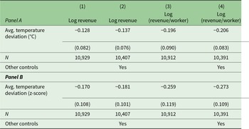
This relationship is further quantified in Table 2, panel A, which shows that a 1°C increase in the 12-month average temperature deviation reduces revenue by approximately 13–14 per cent (column 1) and revenue per worker by approximately 20–21 per cent (column 3). Adding a set of covariates improves the precision of the estimates as reflected by the decreasing standard error but does not significantly change the magnitude of the estimates. This suggests that temperature is exogenous conditional on subdistrict and year-month FE. This estimate represents the total effect of temperature shocks, capturing all pathways through which temperature impacts productivity, including changes in working conditions, worker health and input adjustments. The higher estimated adverse impacts of temperature shock on revenue per worker than on total revenue is a hint that input reallocation might be an important channel. This possibility is explored further in a later section. Further subsample analysis also shows that this adverse impact of temperature shock happens to household businesses both in rural and urban areas, with the former experiencing relatively milder impacts compared to the latter (see Appendix Table A5).
The effect of temperature shocks on household business productivity
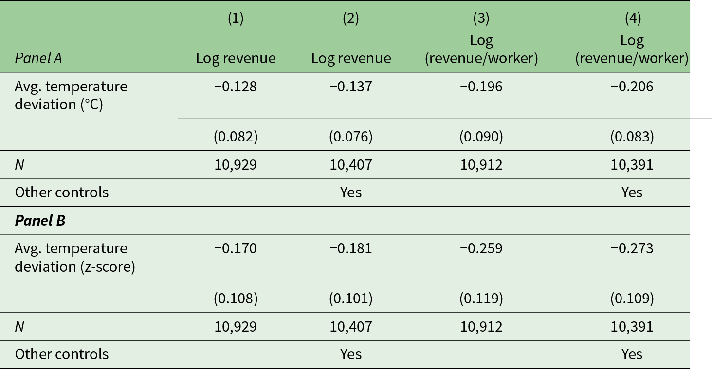
Notes: Standard errors, clustered at temperature grid level, are in parentheses. All the temperature variables are an average of 12 months preceding the survey. All models control for precipitation and include subdistricts FE, year-month FE and business order FE. Other controls include business age, business age squared, location (home-based vs partially home-based vs outside home) dummies and sector dummies.
Considering actual temperature deviation variation in the sample, panel B shows that a one standard deviation increase in average temperature deviation decreases revenue by 18 per cent and revenue per worker by 27 per cent. These effects are higher compared to panel A since the standard deviation of temperature deviation is higher than 1°C. Together, these findings highlight the rising temperatures’ strong negative impact on household business productivity.
Previous studies that focus on the effect of temperature on output typically find that each degree Celsius rise in average temperature decreases output by around 1–3 per cent (see, e.g., Dell et al., Reference Dell, Jones and Olken2014; Somanathan et al., Reference Somanathan, Somanathan, Sudarshan and Tewari2021) and rarely exceeds 5 per cent. Our finding of a 14 per cent revenue drop, therefore, lies in the upper extreme. We argue that this estimated effect can be reconciled with the literature using the following reasons. Firstly, our sample consists mostly of microenterprises (with an average of only two workers), whereas previous studies typically focus on macro data (driven largely by large businesses) or on large firms directly. Smaller firms have fewer resources to cope with temperature shocks and therefore experience more severe adverse impacts. Secondly, because smaller businesses have lower revenues, even a modest change in revenue levels can translate into a large percentage change. In fact, the mean annual revenue of household businesses in our sample is only around US$1,000–3,000 in 2024 dollars (see Appendix Table A6).
As the outcome is measured for a 1-year period, it is possible that during this time span, household businesses adapt to temperature shocks in ways that could dampen the adverse impacts. Among the possible adaptation strategies are input reallocation and relocation of businesses (migration). Firstly, if input reallocation (changing the capital and labour mix) were carried out optimally, it would mitigate the negative effect of temperature on output. We test this by regressing total revenue on temperature while controlling for labour and capital inputs (under both Cobb–Douglas and Translog specifications). If optimal adaptation were occurring, we would expect that the inclusion of labour and capital in the regression would mimic the inability to reallocate inputs, thereby amplifying the measured effect of temperature. As shown in Appendix Table A7, controlling for labour and capital inputs does amplify the negative effect. However, the changes in magnitudes are only marginal. Secondly, household businesses might adapt to temperature change by relocating their business to other areas. However, we have shown in the threats to identification section that business owner migration is uncorrelated with temperature shocks, thus ruling out this adaptation mechanism.
5.2. Nonlinearity of temperature effect
Previous studies found a nonlinear effect of temperature on productivity (see, e.g., Dasgupta et al., Reference Dasgupta, Maanen, Gosling, Piontek, Otto and Schleußner2021; Somanathan et al., Reference Somanathan, Somanathan, Sudarshan and Tewari2021; Tarsia, Reference Tarsia2024). We check the possibility of nonlinear effects by modifying our models.
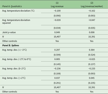
Panel A of Table 3 explores the potential nonlinearity in the relationship between temperature and revenue per worker by incorporating a quadratic function of average temperature into the analysis. The results indicate that the relationship follows an inverted U-shape. This finding is supported by the joint significance test, where the p-value is below 5 per cent in both outcomes, confirming the statistical relevance of the quadratic term. These results suggest that while moderate temperatures are conducive to productivity, deviations on either side of the optimal temperature have negative impacts, highlighting the delicate balance between environmental conditions and labour performance. This inverted-U relationship aligns with findings from Dasgupta et al. (Reference Dasgupta, Maanen, Gosling, Piontek, Otto and Schleußner2021) and Tarsia (Reference Tarsia2024). Further sectoral analysis (see Appendix Table A8) shows that this nonlinear relationship exists in secondary (manufacturing and construction) and tertiary (services and trade) sectors, but that there is no evidence of any relationship in the primary sector (agriculture, forestry, fishing and mining).
Nonlinear effect of temperature shocks on worker productivity
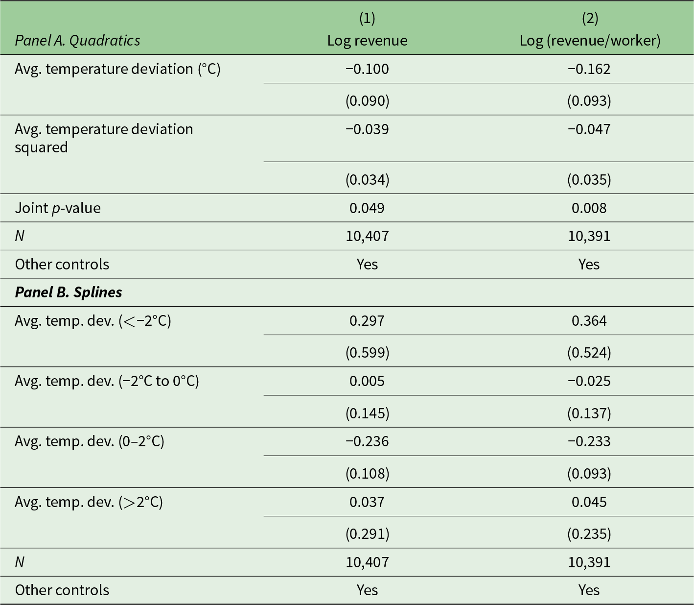
Notes: Standard errors, clustered at temperature grid level, are in parentheses. All the temperature variables are the average of 12 months preceding the survey. All models control for precipitation and include subdistricts FE, year-month FE and business order FE. Other controls include business age, business age squared, location (home-based vs partially home-based vs outside home) dummies and sector dummies.
Panel B of Table 3 employs an alternative approach using spline regression to examine the temperature–productivity relationship further. The analysis reveals that when temperature deviations are below −2°C from the LTM, temperature increases actually improve productivity. The statistical significance is absent, however, because of the relatively small number of observations (fewer than 600 observations coming from only 12 different grids) in this temperature category. Since the average temperature LTM is around 26.5°C, this temperature range corresponds to the temperature levels below 24.5°C. This result suggests the potential benefits of temperature increases in suboptimal (cooler) conditions. In the temperature deviation range of −2°C to 0°C, the temperature effect is relatively flat. Then, in the next temperature deviation range of 0–2°C (corresponding to a temperature level of around 26.5–28.5°C), temperature increase starts to have adverse impacts on productivity. The last temperature deviation range (>2°C) shows no statistically significant effect, but this is due to low observations (fewer than 600 observations coming from only 19 different grids) and hence very low precision (the standard deviations in both models are more than five times higher than the coefficients). This finding aligns with the quadratic model results and suggests that the adverse effects of high temperatures intensify as temperatures rise.
5.3. Mechanism
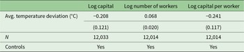
In the previous section, we showed that the effect of temperature shocks on revenue per worker is higher than on total revenue. This fact suggests the existence of input reallocation effect of temperature shocks. We now explicitly check this plausibility by using log capital, log employment and log capital per worker as our outcome in the main regression model.
Table 4 examines how household-based enterprises adjust input usage in response to temperature increases. The results show that higher temperatures significantly increase labour and, on the other hand, decrease physical capital. Combining the two effects, positive temperature shocks significantly decrease capital per worker. This increasing employment effect is consistent with the more pronounced adverse effect of temperature shocks on revenue per worker than on total revenue.
The effects of temperature shocks on capital, employment and capital per worker
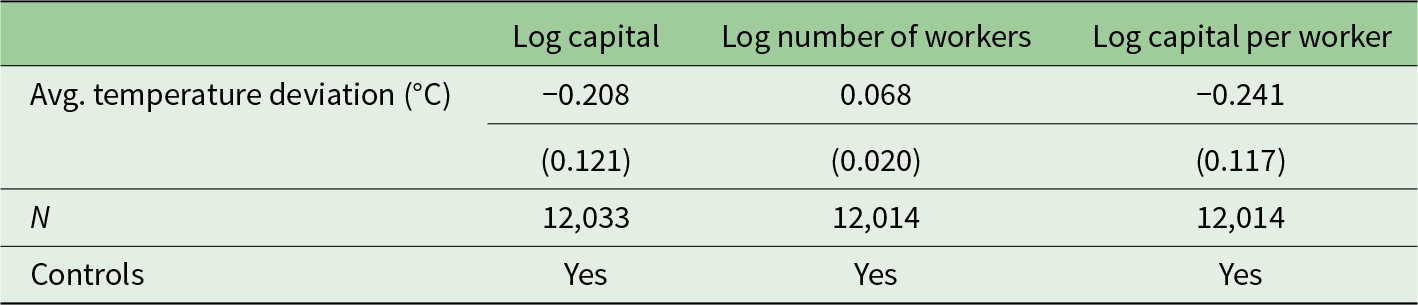
Notes: Standard errors, clustered at temperature grid level, are in parentheses. All the temperature variables are an average of 12 months preceding the survey. All models control for precipitation and include subdistricts FE, year-month FE and business order FE. Other controls include business age, business age squared, location (home-based vs partially home-based vs outside home) dummies and sector dummies.
The observed reduction in capital use alongside an increase in labour input during periods of extreme heat can be interpreted through two main mechanisms. One possibility is input substitution. If capital and labour are substitutable, extreme temperatures may induce household businesses to re-optimize their input mix by relying more on labour while reducing capital use. However, this interpretation would imply an increase in labour productivity during heat shocks, which contradicts a substantial body of evidence showing that extreme heat reduces worker productivity (see, e.g., Somanathan et al., Reference Somanathan, Somanathan, Sudarshan and Tewari2021). For this reason, a pure substitution story driven by rising labour productivity appears unlikely.
A more consistent explanation is that labour productivity declines during extreme heat, but labour input nevertheless increases because the effective price of labour falls. Extreme weather events are associated with higher unemployment and reduced labour demand in larger firms (Rujiwattanapong and Yoshida, Reference Rujiwattanapong and Yoshida2025), which can increase the supply of labour available to household-based businesses. In this context, informal household enterprises may function as employers of last resort, absorbing excess labour at lower wages and compensating for reduced productivity by employing more workers.
The observed decline in capital use should be interpreted with caution. Unlike labour, which is measured in physical units (number of workers), capital in our data is proxied by the monetary value of business assets. Changes in asset values do not necessarily correspond to changes in the physical quantity of capital. The decline in measured capital may therefore reflect reduced utilization or effectiveness of physical capital during extreme heat, rather than an actual reduction in capital stock. Alternatively, it may indicate the liquidation of business assets as a coping strategy to mitigate income losses during periods of extreme temperature. While our data do not allow us to distinguish conclusively between these channels, both interpretations are consistent with household businesses adjusting to adverse environmental shocks.
5.4. Heterogeneity of effect
In this section, we further explore the potential heterogeneous effect of temperature shocks on revenue per worker across different temperature LTM, employment and capital, as well as across sectors.
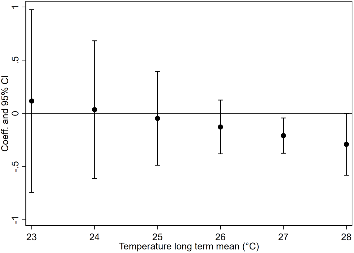
Figure 2 examines whether the impact of temperature shocks on revenue per worker varies depending on a region’s ‘normal’ temperature, which is proxied by the LTM temperature. The analysis reveals that areas with higher normal temperatures experience a greater adverse effect on revenue per worker from the same magnitude of temperature increase. This finding suggests that hotter regions are more vulnerable to temperature shocks, as they are already closer to thresholds where further increases significantly impair productivity. This is in line with previous macro-level studies, which found that countries with already-warm climates will pay the highest price of global warming (Dell et al., Reference Dell, Jones and Olken2014). These results emphasize the disproportionate risks businesses face in hotter areas, underscoring the need for targeted interventions to mitigate the effects of rising temperatures in these regions.
The effect of temperature shocks on worker productivity by temperature LTM.
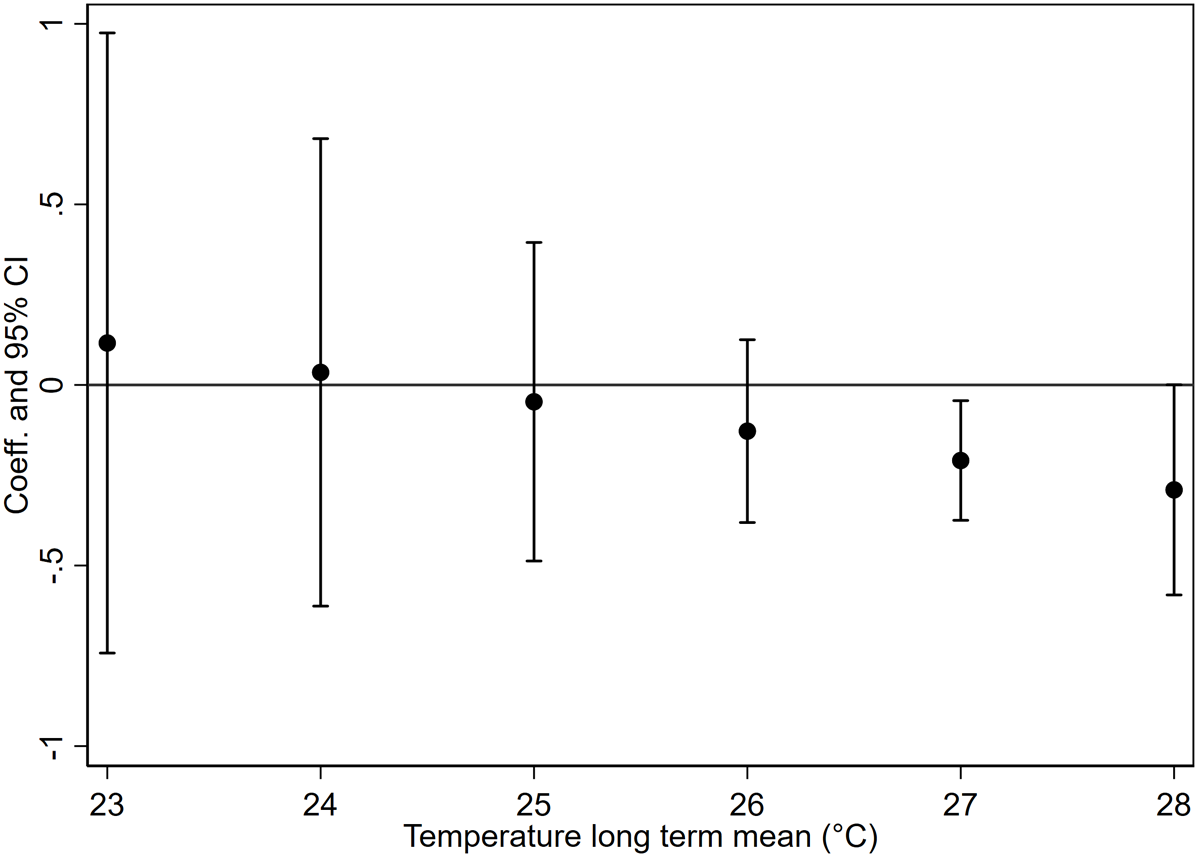
Figure 3A explores the effect of temperature shocks on business size, measured in terms of employment. The results indicate that temperature increases of the same magnitude disproportionately adversely impact revenue per worker in smaller businesses. For businesses with 10 or more workers, the effect of temperature shocks is statistically insignificant, as the null hypothesis of no effect cannot be rejected. However, since most household-based enterprises in the sample are micro and small businesses – with an average of just over two workers – these findings highlight the vulnerability of smaller businesses to temperature shocks. This unequal impact can potentially exacerbate existing economic inequalities, as smaller, already resource-constrained businesses bear the brunt of climate-induced productivity losses.
The effect of temperature shocks on worker productivity by the number of workers and the value of capital.

Figure 3B shows whether the impact of temperature shocks on revenue per worker varies with business size in terms of capital. While the effect appears slightly larger for businesses with higher capital, the difference is negligible. Simpler regressions that include interaction terms between average temperature deviation and capital show that this interaction term is not statistically significant. This indicates that the adverse effect of temperature shocks on revenue per worker is consistent across businesses of different capital sizes. Thus, temperature shocks affect businesses in a relatively uniform way regardless of their scale in terms of capital, emphasizing that capital size does not mitigate the vulnerability to temperature-induced productivity losses.
Figure 4 explores the differential impact of temperature shocks on revenue per worker across various sectors. The results show that the construction sector is the most adversely affected. However, the confidence interval for this estimate is also wide due to a very small sample size. The manufacturing and food sales sectors are the next most impacted, experiencing around a 22–28 per cent drop in revenue per worker for every 1°C increase in temperature. These are followed by the agriculture, non-food sales and services sectors, which experience a smaller decline of around 17–20 per cent.
The effect of temperature shocks on worker productivity by business sector.

In contrast, the agriculture, transportation and communication, as well as finance, insurance and real estate sectors show no statistically significant effect from temperature shocks. The mining and quarrying sector also displays no significant impact, possibly due to a limited sample size. These findings suggest that sectors with higher physical labour demands are particularly vulnerable to temperature-induced productivity losses, while more service-oriented industries appear less sensitive. It should also be noted that workers in sectors such as communications, finance and real estate are more likely to have access to climate control devices (such as air conditioning) and hence evade the temperature shock effects.
5.5. Robustness checks
Our main results are robust to a battery of tests. Firstly, the results are robust to the inclusion of more fine-grained FE. Ideally, firm FE should be used. However, since there is no identifier to match household businesses across IFLS rounds, we make use of two available alternatives. Table A9 in the Appendix shows that the estimated coefficients are still negative and significant when we include household FE or business managers’ FE.
Secondly, our results are robust to the use of alternative temporal FE. Panel A of Table A10 in the Appendix shows that when we change the FE from year-month to year and month separately, the coefficients are still negative and significant. Panel B of the same table shows that when we use province-year-month FE, the magnitude is still negative, while the statistical significance is gone due to imprecision caused by the fact that our temperature only varies across subdistricts, yet there are only a few subdistricts within each province in our sample.
Thirdly, several studies of temperature shock effects use a nonparametric specification for the temperature variable by using counts of daily maximum temperature in several intervals (bins) to allow for nonlinear effects. We check the robustness of our main result using this approach. Table A11 in the Appendix shows the regression results for two alternative bin sizes (2C and 3C). Despite the loss of precision, the estimates suggest an inverse-U pattern: moving one day with maximum temperature from the lowest bin into warmer bins initially increases productivity, but further warming brings productivity back to a level statistically indistinguishable from the lowest bin. Overall, we can say that the effect of temperature shock on productivity is at least linear, with a possibility of an inverse-U effect.
Fourthly, in Appendix Table A12, we show that our results are robust when we restrict our sample to only include balanced panel households, i.e., only containing households that own businesses in all three rounds (IFLS 3, 4 and 5). The regression results for both revenue and revenue per worker outcome are still significant, even with a bigger absolute magnitude. This also addresses the concern about systematic attrition that we have discussed in the threats to identification section. Lastly, in Appendix Table A13, we show that our results are also robust when we use different measures of employment, from including all workers to only including paid workers.
6. Conclusion and recommendations
This study demonstrates a clear and robust negative relationship between rising temperatures and productivity in Indonesia’s household-based enterprises. A 1°C increase in the 12-month average temperature reduces revenue by 14 per cent and revenue per worker by 21 per cent, reflecting the significant total effect of temperature on productivity. Furthermore, we also found the inverted U-shaped relationship, with productivity peaking at around 25–26°C.
Our findings also reveal that micro and small enterprises, particularly those in hotter regions and labour-intensive sectors like construction and manufacturing, are disproportionately affected by temperature increases. Conversely, larger businesses and less labour-intensive sectors show greater resilience, widening the productivity gap and potentially exacerbating economic inequality. This evidence underscores the vulnerabilities of small-scale enterprises to climate change and the urgent need for targeted support.
From the results, we propose several policy recommendations that are not just applicable to Indonesia, but also to emerging countries in tropical areas with a significant portion of micro and small enterprises in the economy. Firstly, enhancing an adaptation strategy for vulnerable enterprises, especially micro and small-sized ones, is urgent. Policymakers in emerging economies should prioritize micro and small businesses in climate adaptation programs by providing financial incentives, technical assistance and training to improve their resilience. We found that they were affected considerably and had limitations on the adjustment side to maintain output. For instance, subsidies for climate-friendly technologies, access to cooling infrastructure and improved working conditions can help mitigate the productivity losses caused by temperature shocks.
Secondly, emerging countries need a sector-specific climate resilience measurement. Labour-intensive sectors, particularly construction, agriculture and manufacturing, require tailored interventions to reduce climate vulnerability. Investments in heat-resilient infrastructure, technological upgrades and innovative farming practices, such as precision agriculture, can enhance productivity while minimizing climate-related risks. Thirdly, governments in emerging economies should improve their regional targeting and equity considerations. Regions with higher baseline temperatures and businesses in hotter areas should be prioritized for climate adaptation programs. Targeted interventions, such as localized cooling solutions, heat-adaptive work schedules and region-specific grants or subsidies, can reduce the disproportionate impact of temperature shocks on these areas. This recommendation applies not only to Indonesia but also to all developing countries near the equator.
Lastly, governments need to put a long-term investment in green technology and climate policy. Policymakers must invest in sustainable and energy-efficient technologies to reduce the impact of rising temperatures. Strengthening commitment to renewable energy, urban greening projects and climate-resilient infrastructure will not only mitigate the adverse effects of temperature increases but also contribute to long-term economic and environmental sustainability. We believe that by adopting these recommendations, Indonesia can help safeguard its labour productivity, reduce economic inequalities and enhance the resilience of its enterprises in the face of rising temperatures.
Supplementary material
The supplementary material for this article can be found at https://doi.org/10.1017/S1355770X26100564.
Acknowledgements
The authors are grateful to Universitas Gadjah Mada, which provided a research grant for this study through the Academic Excellence Grant Program with ID (6529/UN1.P1/PT.01.03/2024). The authors thank the Editor and two anonymous referees for helpful comments. The authors also thank Ardina Hasanbasri, Albert Park, Dorothea Ramizo, Yanrui Wu and participants of the 2025 Asian Economic Development Conference for their valuable comments on the earlier version of the paper. Special thanks to Muhammad Putra, Mikael Bagas Ario Wicaksono and Ester Dwi Sabtu for their excellent research assistance.
Competing interests
The authors declare none.