1 Introduction
Newton’s method, also known as the Newton–Raphson method named after Isaac Newton (1642–1727) and Joseph Raphson (1648–1715), is probably the oldest and most famous iterative process to be found in mathematics. The method was first proposed to find successively better approximations to the roots (or zeros) of a real-valued function
 $p(z)$
. Picking an initial point
 $z_0$
near a root of p, Newton’s method produces an nth approximation of the root via the formula
 $z_{n+1}=f_p(z_n)$
, where
 $$ \begin{align*}f_p(z)=z-\frac{p(z)}{p'(z)}\end{align*} $$
is called the Newton map of p. Replacing
 $z_n$
by
 $z_{n+1}$
generates a sequence of approximations
 $\{z_n\}$
which may or may not converge to a root of p.
A brief history of Newton’s method, following [Reference AlexanderA], is as follows. Versions of Newton’s method had been in existence for centuries previous to Newton and Raphson. Anticipations of Newton’s method are found in an ancient Babylonian iterative method of approximating the square root of a,
 $$ \begin{align*}z_{n+1}=\frac{1}{2}\bigg(z_n+\frac{a}{z_n}\bigg),\end{align*} $$
which is equivalent to Newton’s method for the function
 $f(z)=z^2-a$
. The modern formulation of the method is also attributed to Thomas Simpson (1710–1761) and Joseph Fourier (1768–1830).
By the mid-1800s, several mathematicians had already examined the convergence of Newton’s method towards the real roots of an equation
 $p(z)=0$
, but the investigations of Ernst Schröder (1841–1902) and Arthur Cayley (1821–1895) are distinguished from their predecessors in their consideration of the convergence of Newton’s method to the complex roots of
 $p(z)=0$
.
Schröder and Cayley each studied the convergence of Newton’s method for the quadratic polynomials, and both showed that on either side of the perpendicular bisector of the roots, Newton’s method converges to the root on that particular side. However, in 1879, Cayley [Reference CayleyC] first noticed the difficulties in generalizing Newton’s method to cubic polynomials, or general polynomials with at least three distinct roots. In [Reference CayleyC], Cayley wrote:
‘The solution is easy and elegant in the case of a quadratic equation, but (Newton’s method for) the next succeeding case of the cubic equation appears to present considerable difficulty.’
The study of Newton’s method led to the theory of iterations of holomorphic functions, as initiated by Pierre Fatou and Gaston Julia around the 1920s. Since then, the study of Newton maps became one of the major themes with general interest, both in discrete dynamical system (pure mathematics), and in root-finding algorithm (applied mathematics), see for example [Reference Aspenberg and RoeschAR, Reference BarańskiBa, Reference BergweilerBe, Reference Baranski, Fagella, Jarque and KarpinskaBFJK1, Reference Baranski, Fagella, Jarque and KarpinskaBFJK2, Reference Hubbard, Schleicher and SutherlandHSS, Reference PrzytyckiPr, Reference RoederRo07, Reference RoeschRo08, Reference Roesch, Wang and YinRWY, Reference Shishikura and SchleicherSh, Reference TanTan].
Let p be a polynomial with at least two distinct roots (the discussion is trivial when p has only one (possibly multiple) root), and let
 $\zeta \in {\mathbb {C}}$
be a root of p. For its Newton map
 $f_p$
, the attracting basin or root basin of
 $\zeta $
, denoted by
 $B(\zeta )$
, consists of points z on the Riemann sphere
 $\widehat {\mathbb {C}}$
whose orbit
 $\{f_p^n(z);n\in \mathbb N\}$
(here
 $g^n$
means the nth iterate of g) converges to
 $\zeta $
:
 $$ \begin{align*}B(\zeta)=\{z\in \widehat{\mathbb{C}}; f^n_p(z)\rightarrow \zeta \text{ as } n\rightarrow +\infty\}.\end{align*} $$
It is well known that
 $B(\zeta )$
is an open set of
 $\widehat {\mathbb {C}}$
. In the case that p has two distinct (possibly multiple) roots, by quasi-conformal surgery, one can show that
 $B(\zeta )$
is a quasi-disk and the Julia set
 $J(f_p)$
is a quasi-circle. So this case is easy.
We say that a polynomial p is non-trivial (in the sense of Cayley) if p has at least three distinct roots. A non-trivial polynomial takes the form
 $$ \begin{align*} p(z)=a(z-a_1)^{n_1}\cdots(z-a_d)^{n_d}, \end{align*} $$
where
 $a\in \mathbb C-\{0\}$
,
 $d\geq 3$
, and
 $a_1,\ldots , a_d\in \mathbb C$
are distinct roots of p, with multiplicities
 $n_1,\ldots ,n_d\geq 1$
. This is the general case and the attracting basin
 $B(\zeta )$
consists of countably many connected components. The one containing
 $\zeta $
is called the immediate attracting basin or immediate root basin, and is denoted by
 $B^0(\zeta )$
. Przytycki [Reference PrzytyckiPr] showed that
 $B^0(\zeta )$
is a topological disk when p is a non-trivial cubic polynomial. By means of quasi-conformal surgery, Shishikura [Reference Shishikura and SchleicherSh] proved that the Julia set of the Newton map for any non-trivial polynomial is connected. This result is further generalized to Newton’s method for entire functions by Baranski et al [Reference Baranski, Fagella, Jarque and KarpinskaBFJK1, Reference Baranski, Fagella, Jarque and KarpinskaBFJK2]. This implies, in particular, each component of
 $B(\zeta )$
is a topological disk.
Although
 $B=B^0(\zeta )$
has a simple topology, its boundary
 $\partial B$
exhibits rich topological structures. The reason is that the Newton map
 $f_p$
can have unpredictable dynamics and complicated bifurcations on
 $\partial B$
. Therefore, for Newton maps, understanding the topology of
 $\partial B$
makes a fundamental and challenging problem from the view point of dynamical system.
Little progress had been made towards the problem until the ground-breaking work of Roesch. In [Reference RoeschRo08], Roesch proved, building on previous works of Head [Reference HeadHe] and Tan [Reference TanTan], that
 $\partial B$
is always a Jordan curve, when p is a non-trivial cubic polynomial and
 $\mathrm {deg}(f_p|_B)=2$
. The proof is the first successful application of the Branner–Hubbard–Yoccoz puzzle theory to rational maps. The puzzle theory has also been developed by Roesch, Wang, and Yin [Reference Roesch, Wang and YinRWY] to study the local connectivity and rigidity phenomenon in parameter space.
The main result of the paper is to give a complete characterization of
 $\partial B$
for the Newton maps for all polynomials.
Theorem 1.1. Let
 $f_p$
be the Newton map for any non-trivial polynomial p. Then the boundary
 $\partial B$
of any immediate root basin B is locally connected. Moreover,
 $\partial B$
is a Jordan curve if and only if
 $\mathrm {deg}(f_p|_B)=2$
.
The theorem implies that the boundary of each component of the root basins is locally connected. Therefore, the boundaries of all components of root basins, for the Newton maps for all polynomials, from the viewpoint of topology, are tame. Our argument also has a byproduct: the Julia set of a non-renormalizable Newton map is always locally connected, which generalizes Yoccoz’s famous theorem to Newton maps.
Our work extends Roesch’s theorem [Reference RoeschRo08, Theorem 6] for cubic Newton maps to Newton maps of arbitrary polynomials.
It is distinguished from Roesch’s work [Reference RoeschRo08] in two ways. First, the invariant graph is different from those in [Reference RoeschRo08]. In our work, we construct only one graph adapted to the puzzle theory: the one generated by the channel graph, while in [Reference RoeschRo08], countably many candidate graphs are provided, and each of them involves very technical construction. Second, each cubic Newton map has only one free critical point, so the puzzle theory in [Reference RoeschRo08] is the same as the quadratic case; however, the Newton maps for higher degree non-trivial polynomials can have more free critical points, and the quadratic puzzle theory does not work here. To deal with this general case, we take advantage of recent developments [Reference Kahn and LyubichKL1, Reference Kahn and LyubichKL2, Reference Kozlovski, Shen and van StrienKSS] in multi-critical polynomial dynamics.
1.1 Organization of the paper
The paper is organized as follows.
In §2, we present some basic facts for Newton maps.
In §3, we develop a method to count the number of poles (counting a suitable multiplicity) for Newton maps in certain domains arising from dynamics. This allows us to construct an invariant graph for Newton maps by an inductive procedure in §4. This graph is used to develop the puzzle theory.
In §5, we introduce the Branner–Hubbard–Yoccoz puzzle theory and sketch the idea of the proof, whose details are carried out in the forthcoming sections. The strategy is deeply inspired by the work of Roesch and Yin [Reference Roesch and YinRY].
To prove the local connectivity of
 $\partial B$
, for each
 $z\in \partial B$
, we define its end
 ${\mathbf e}(z)$
as the intersection of infinitely many nested puzzle pieces containing z. The main point is to show that
 ${\mathbf e}(z)\cap \partial B=\{z\}$
. For this purpose, we need to treat two cases: the wandering case and the renormalizable case.
In §6, we will show that each wandering end is a singleton. This is based on the dichotomy: a wandering end
 ${\mathbf e}$
either satisfies the bounded degree property or its combinatorial limit set
 $\omega ({\mathbf e})$
contains a persistently recurrent critical end. The treatments for these two cases are different: the former needs to control the number of critical points in long orbits of puzzle pieces, while the latter makes essential use of recent developments in multi-critical polynomial dynamics, especially the principle nest construction and its properties [Reference Kahn and LyubichKL1, Reference Kahn and LyubichKL2, Reference Kozlovski, Shen and van StrienKSS].
In §7, we handle the renormalizable case. We will show that if
 ${\mathbf e}(z)$
is periodic and non-trivial, then
 ${\mathbf e}(z)\cap \partial B=\{z\}$
. The main idea is to construct an invariant curve which separates the end
 ${\mathbf e}(z)$
from B. The construction is natural and less technical (compare [Reference RoeschRo08]). The idea is new and can be applied to study other rational maps.
In §8, we complete the proof of the main theorem.
1.2 Notation
Throughout the paper, we will use the following notation.
-
(1)
 $\widehat {\mathbb {C}}$
,
${\mathbb {C}}$
, and
$\mathbb {D}$
are the Riemann sphere, the complex plane, and the unit disk, respectively. The boundary of
$\mathbb {D}$
is denoted by
$\mathbb {S}$
.
-
(2) Let A be a set in
$\widehat {\mathbb {C}}$
. The closure and the boundary of A are denoted by
$\overline {A}$
and
$\partial A$
, respectively. We denote by
$\mathrm {Comp}(A)$
the collection of all connected components of A. The cardinality of A is
$\#A$
. -
(3) Given two subsets A and B of
$\widehat {\mathbb {C}}$
, we say that
$A\Subset B$
if A is contained in the interior of B. -
(4) The Julia set and Fatou set of a rational map f are denoted by
$ J(f)$
and
$ F(f)$
, respectively.


2 Preliminaries
This section collects some basic facts and introduces some notation for Newton maps.
Let p be a complex polynomial, factored as
 $$ \begin{align*}p(z)=a(z-a_1)^{n_1}\cdots(z-a_d)^{n_d},\end{align*} $$
where
 $a\neq 0$
and
 $a_1,\ldots , a_d\in \mathbb {C}$
are distinct roots of p, with multiplicities
 $n_1,\ldots , n_d\geq ~1$
. In our discussion, we may assume
 $d\geq 2$
.
Its Newton map
 $f_p$
fixes each root
 $a_k$
with multiplier
 $$ \begin{align*}f_p'(a_k)=\frac{p(z)p''(z)}{p'(z)^2}\bigg|_{z=a_k}=\frac{n_k-1}{n_k}.\end{align*} $$
Therefore, each root
 $a_k$
of p corresponds to an attracting fixed point of
 $f_p$
with multiplier
 $1-1/n_k$
. It follows from the equation
 $$ \begin{align*}\frac{1}{f_p(z)-z}=-\sum_{k=1}^d\frac{n_k}{z-a_k}\end{align*} $$
that the degree of
 $f_p$
equals d, the number of distinct roots of p. One may also verifies that
 $\infty $
is a repelling fixed point of
 $f_p$
with multiplier
 $$ \begin{align*}\lambda_\infty=\frac{\sum_{k=1}^d n_k}{\sum_{k=1}^d n_k-1}=\frac{\deg(p)}{\deg(p)-1}.\end{align*} $$
From the above discussion, we see that a degree-d Newton map has
 $d+1$
distinct fixed points with specific multipliers. However, a well-known theorem of Head states that the fixed points together with the specific multipliers can determine a unique Newton map.
Theorem 2.1. (Head [Reference HeadHe])
A rational map f of degree
 $d\geq 2$
is the Newton map of a polynomial p if and only if f has
 $d+1$
distinct fixed points
 $$ \begin{align*}a_1, a_2, \ldots, a_d, \infty,\end{align*} $$
such that for each fixed point
 $a_k$
, the multiplier takes the form
 $$ \begin{align*}f'(a_k)=1-1/n_k \quad\text{with } n_k\in \mathbb N, \ 1\leq k\leq d.\end{align*} $$
In this case, the polynomial p has the form
 $a(z-a_1)^{n_1}\cdots (z-a_d)^{n_d}, \ a\neq 0$
.
Now, for the Newton map
 $f=f_p$
of p, let
 $B(a_k)$
be the root basin of
 $a_k$
and
 $B_k$
be the immediate root basin of
 $a_k$
. Recall that
 $$ \begin{align*}B(a_k)=\{z\in \widehat{\mathbb{C}}; f^n(z)\rightarrow a_k \text{ as } n\rightarrow +\infty\}.\end{align*} $$
The attracting basin for all roots is
 $$ \begin{align*}{B}_f=B(a_1)\cup\cdots\cup B(a_d).\end{align*} $$
We say that f is post-critically finite in
 ${B}_f$
if there are only finitely many post-critical points in
 $B_f,$
or equivalently, each critical point in
 ${B}_f$
will eventually be iterated to one critical point of
 $a_k$
.
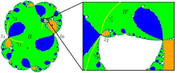
According to Shishikura [Reference Shishikura and SchleicherSh], the Julia set of a Newton map f is always connected, or equivalently, all Fatou components of f are simply connected (see Figure 1). By means of quasi-conformal surgery, one can show that f is quasi-conformally conjugate, in a neighborhood of of
 $\mathbb {\widehat {C}}-B_f$
, to a Newton map g which is post-critically finite in its root basin
 $B_g$
. Because the topology of the Julia set
 $J(f)$
does not change under this conjugacy, throughout the paper, we pose the following.
Image of the Julia set
 $J(f)$
under the action of the Möbius map
 $h(z)={z}/({z-1})$
, where f is the Newton map for the polynomial
 $p(z)=(z^2-1)(z-a)(z-b)$
with
 $a=-1.142-2.0477\,i$
and
 $b=0.1667-3.15485\,i$
.

Assumption 2.2. The Newton map f is post-critically finite in
 $B_f$
.
Under Assumption 2.2, if the degree d of f is two, then f is affinely conjugate to
 $z^2$
. In this case, the collection
 $\mathrm {Comp}(B_f)$
of all components of
 $B_f$
consists of only two elements. In other situations,
 $\mathrm {Comp}(B_f)$
consists of infinitely many elements.
A virtue of Assumption 2.2 is that one can give a natural dynamical parameterization of root basins (see [Reference MilnorMi06]).
Lemma 2.3. Assume f is post-critically finite in
 $B_f$
, then there exist so-called Böttcher maps,
 $\{\Phi _B\}_{B\in \mathrm {Comp}({B}_f)}$
, such that for each
 $B\in \mathrm {Comp}({B}_f)$
:
-
(1)
$\Phi _B:B\to \mathbb {D}$
is a conformal map; -
(2)
$\Phi _{f(B)}\circ f\circ \Phi _B^{-1}(z)=z^{d_{B}}, \text { for all } z\in \mathbb {D}$
, where
$d_B=\mathrm {deg}(f|_{B})$
.


In general, for each
 $B\in \mathrm {Comp}({B}_f)$
, the Böttcher map
 $\Phi _B$
is not unique. There are
 $d_B-1$
choices of
 $\Phi _B$
when
 $f(B)=B$
, and
 $d_B$
choices of
 $\Phi _B$
when
 $f(B)\neq B$
and
 $\Phi _{f(B)}$
is determined. Once we fix a choice of Böttcher maps
 $\{\Phi _B\}_{B\in \mathrm {Comp}({B}_f)}$
, we may define the internal rays, as follows.
For each
 $B\in \mathrm {Comp}({B}_f)$
, the point
 $\Phi _B^{-1}(0)$
is called the center of B, and the Jordan arc
 $$ \begin{align*}R_B(\theta):=\Phi_B^{-1}(\{re^{2\pi i\theta}:0<r<1\})\end{align*} $$
is called the internal ray of angle
 $\theta $
in B. According to a well-known landing theorem [Reference MilnorMi06, Theorem 18.10], when
 $\theta $
is rational, the internal ray
 $R_B(\theta )$
always lands (that is the limit
 $\lim _{r\rightarrow 1^-} \Phi _B^{-1}(re^{2\pi i\theta })$
exists). A number
 $r\in (0,1)$
and two rational angles
 $\theta _1,\theta _2$
induce a sector:
 $$ \begin{align*}S_B(\theta_1,\theta_2;r):=\Phi_B^{-1}(\{t\,e^{2\pi i\theta}:r<t<1,\theta_1<\theta<\theta_2\}),\end{align*} $$
here
 $\theta _1<\theta <\theta _2$
means that the angles
 $\theta _1, \theta , \theta _2$
sit in the circle in the counter clock-wise order.
3 Counting number of poles
In this section, we develop a method to count the number of poles (counting suitable multiplicity) for Newton maps f in certain domains (which arise from dynamics). We will show that in the domains we consider, the number of poles is strictly less than the number of Jordan curves which bound the domain. This fact allows us to construct an invariant graph for Newton maps by an inductive procedure (see §4).
3.1 Counting number of fixed points
By a graph we mean a connected and compact subset of
 $\widehat {\mathbb {C}}$
, written as the disjoint union of finitely many points (called vertices) and finitely many open Jordan arcs (called edges), any two of which touch only at vertices. A graph can contain a loop.
Let G be a graph. For any
 $z\in G$
, let
 $\nu (G, z)$
be the number of components of
 $G\setminus \{z\}$
. We call z a cut point of G if
 $\nu (G, z)\geq 2$
(
 $\Longleftrightarrow \, G\setminus \{z\}$
is disconnected), a non-cut point of G if
 $\nu (G, z)=1$
(
 $\Longleftrightarrow \, G\setminus \{z\}$
is connected). Observe that all components in
 $\widehat {\mathbb {C}}\setminus G$
are Jordan disks if and only if all
 $z\in G$
are non-cut points.
In our discussion, by a Jordan domain or Jordan disk, we mean an open subset of
 $\widehat {\mathbb {C}}$
whose boundary is a Jordan curve. A pre-Jordan domain W means a connected component of
 $g^{-1}(D)$
, where D is a Jordan disk and g is a rational map. Here the boundary
 $\partial D$
may or may not contain critical values of g. If
 $\partial D$
contains no critical value of g, then each boundary component of W is a Jordan curve; if
 $\partial D$
contains at least one critical value of g, then each component of
 $\partial W$
can be written as a union of finitely many Jordan curves, touching at critical points. In either case, for any component
 $\gamma $
of
 $\partial W$
, the map
 $g|_{\gamma }: \gamma \rightarrow \partial D$
has a well-defined degree, denoted by
 $\mathrm {deg}(g|_\gamma )$
. It is equal to the number of preimages
 $g^{-1}(q)$
on
 $\gamma $
of a point
 $q\in \partial D$
which is not a critical value.
One may observe that for any pre-Jordan domain W, any component V of
 $h^{-1}(W)$
is again a pre-Jordan domain, here h is a rational map. To see this, note that W is a component of
 $g^{-1}(D)$
(D is a Jordan disk) and V is a component of
 $(g\circ h)^{-1}(D)$
, where
 $g\circ h$
is a rational map.
Let U be a pre-Jordan domain and D be a Jordan disk in
 $\widehat {\mathbb {C}}$
such that
 $U\subseteq D$
. The filled closure of U with respect to D, denoted by
 $\widehat {U}_D$
, is
 $$ \begin{align*}\widehat{U}_D=\overline{U}\cup\bigcup_V\overline{V},\end{align*} $$
where V ranges over all components of
 $\widehat {\mathbb {C}}\setminus \overline {U}$
with
 $V\subseteq D$
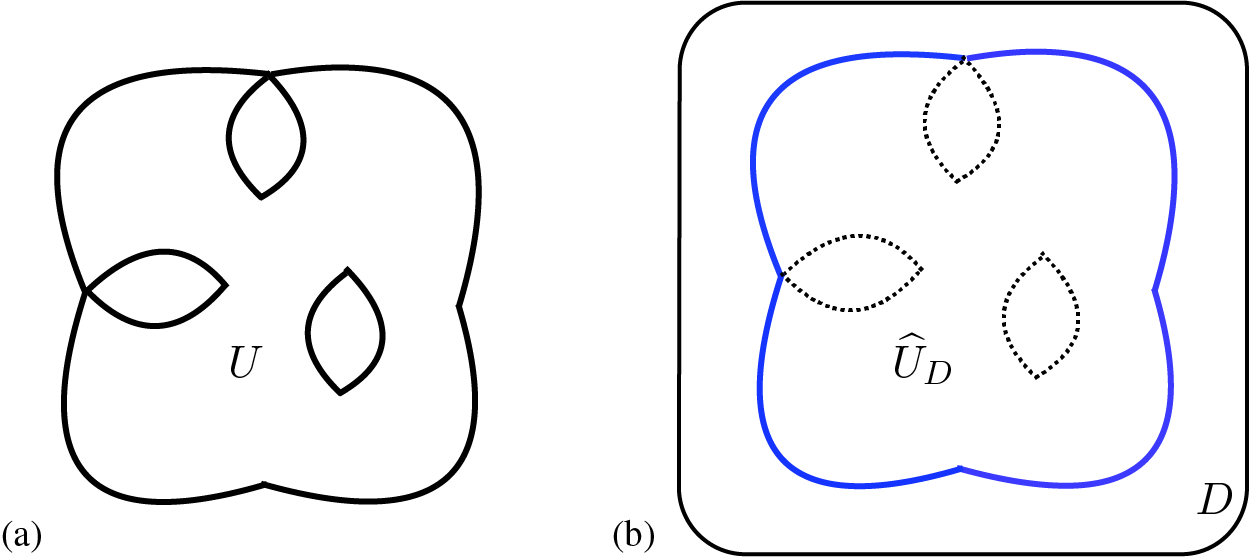
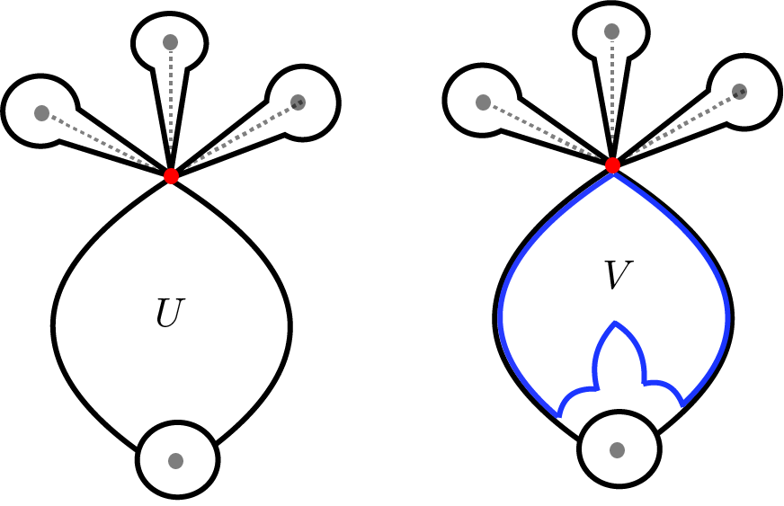
. See Figure 2.
An example of pre-Jordan domain U (a) and its filled closure
 $\widehat {U}_D$
with respect to D (b). Clearly
 $\widehat {U}_D$
is a Jordan disk bounded by a blue curve.

It is easy to verify the following facts.
-
(1)
$\overline {U}\subseteq \widehat {U}_D\subseteq \overline {D}$
and
$\widehat {U}_D=\widehat {U}_{D'}$
for any Jordan disk
$D'$
containing D. -
(2) The filled closure
$\widehat {U}_D$
is always a Jordan disk. To see this, if
$\widehat {U}_D$
is not a Jordan disk, then
$\partial \widehat {U}_D$
is not a Jordan curve, and can be written as a union of finitely many Jordan curves, say
$\alpha _1, \ldots , \alpha _k$
with
$k\geq 2$
, such that the intersection of any two curves is a finite set. These curves enclose mutually disjoint Jordan disks,
$D_1, \ldots , D_k$
, in
$\widehat {\mathbb {C}}-\overline {U}$
. Note that
$\partial D\subset \overline {D}_j$
for some j, however this will contradict the definition of
$\widehat {U}_D$
. -
(3)
$\widehat {U}_D=\overline {U}$
if and only if U is a Jordan disk.


The following fixed point theorem appears in [Reference Rückert and SchleicherRS, Theorem 4.8].
Lemma 3.1. Let
 $D\subseteq \widehat {\mathbb {C}}$
be a Jordan disk and g be a rational map of degree at least two. Suppose that
 $g^{-1}(D)$
has a component
 $U\subseteq D$
. If
 $\partial D\cap \partial U$
contains a fixed point q, we further require that q is repelling and
 $g(N_q\cap \partial U)\supseteq N_{q}\cap \partial U$
in a neighborhood
 $N_{q}$
of q. Then
 $$ \begin{align*}\#\mathrm{Fix}(g|_{\overline{U}})=\mathrm{deg}(g|_{\partial U}).\end{align*} $$
Here the number of fixed points is counted with multiplicity. Recall that the multiplicity of a fixed point
 $z_0\in \mathbb C$
is defined to be the unique integer
 $m\geq 1$
such that, near
 $z_0$
,
 $$ \begin{align*}g(z)-z=a_m(z-{z}_0)^m+a_{m+1}(z-{z}_0)^{m+1}+\cdots\end{align*} $$
with
 $a_m\neq 0$
. The number m is independent of the choice of coordinates.
As a consequence of Lemma 3.1, one has the following corollary.
Corollary 3.2. Let D be a Jordan disk in
 $\widehat {\mathbb {C}}$
and g be a rational map of degree at least two. Suppose that
 $g^{-1}(D)$
has a component
 $U\subseteq D$
. If
 $\partial D\cap \partial U$
contains a fixed point q, we further require that q is repelling and
 $g(N_q\cap \partial U)\supseteq N_{q}\cap \partial U$
in a neighborhood
 $N_{q}$
of q. Then
 $$ \begin{align*}\#\mathrm{Fix}(g|_{\widehat{U}_D})=\sum_{V}\mathrm{deg}(g|_{\partial V}),\end{align*} $$
where V runs over all components of
 $g^{-1}(D)$
such that
 $V\subseteq \widehat {U}_D$
.
In particular, if
 $\widehat {U}_D$
contains only one fixed point (counting multiplicity), then U is a Jordan disk (
 $\Longleftrightarrow \,\overline {U}=\widehat {U}_D$
) and
 $g:U\to D$
is a homeomorphism.
Proof. Let
 $V_1=U, V_2,\ldots ,V_n$
(respectively
 $V^{\prime }_1,\ldots ,V_m'$
) be all the components of
 $g^{-1}(D)$
(respectively
 $g^{-1}(\widehat {\mathbb {C}}\setminus \overline {D})$
) in the filled closure
 $\widehat {U}_D$
. Then by definition,
 $$ \begin{align*}\widehat{U}_D=\overline{V}_1\cup\cdots\cup\overline{V}_n\cup V_1'\cdots\cup V_m'.\end{align*} $$
These
 $V_k'$
terms are clearly disjoint from fixed points. For distinct
 $\overline {V}_i,\overline {V}_j$
, the intersection
 $\overline {V}_i\cap \overline {V}_j$
is a finite set because it is contained in the critical set of g. Further, if
 $\overline {V}_i\cap \overline {V}_j$
contains a fixed point, say q, of g, then q is a critical point and hence a superattracting fixed point. Moreover, we have
 $q\in \partial V_i\cap \partial D$
, and this implies that q is also on
 $\partial U\cap \partial D$
. However, this contradicts our assumption. Therefore, there is no fixed point on
 $\partial V_i\cap \partial V_j$
.
It follows from Lemma 3.1 that
 $$ \begin{align*}\#\mathrm{Fix}(g|_{\widehat{U}_D})=\sum_{1\leq k\leq n}\#\mathrm{Fix}(g|_{\overline{V}_k})=\sum_{1\leq k\leq n}\mathrm{deg}(g|_{\partial V_k}).\end{align*} $$
This equality implies that if
 $\#\mathrm {Fix}(g|_{\widehat {U}_D})=1$
, then U is the unique component of
 $g^{-1}(D)$
in D and
 $\mathrm {deg}(g|_U)=1$
, which proves the statement.
Remark 3.3. What is multiplicity?
In Corollary 3.2, the sum
 $$ \begin{align*}\sum_{1\leq k\leq n}\mathrm{deg}(g|_{\partial V_k})\end{align*} $$
is the cardinality
 $\#(g^{-1}(q)\cap \widehat {U}_D)$
for (any)
 $q\in \partial {D}$
, counting multiplicity.
The multiplicity
 $m(p, \widehat {U}_D)$
of
 $p\in g^{-1}(q)\cap \widehat {U}_D$
is an integer between
 $1$
and the local degree
 $\mathrm {deg}(g,p)$
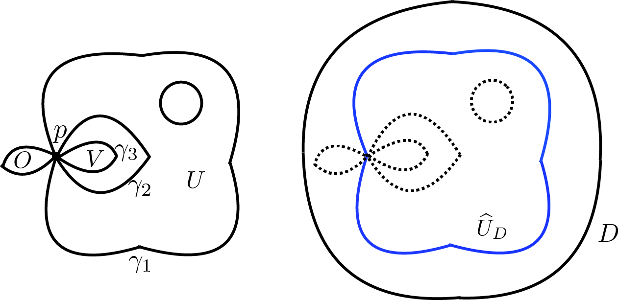
. A natural definition is as follows (see Figure 3).
In this example, there are three components of
 $g^{-1}(D)$
contained in D. They are
 $U, V$
, and O. Their boundaries touch at p. The filled closure
 $\widehat {U}_D$
contains
 $U,V$
. Clearly,
 $\partial U=\gamma _1\cup \gamma _2$
,
 $\partial V=\gamma _3$
. Moreover,
 $\partial U$
meets p twice and
 $\partial V$
meets p once, and hence
 $m(p, \widehat {U}_D)=2+1=3$
. Note also
 $\alpha (p)=\gamma _1\cup \gamma _2\cup \gamma _3$
and
 $\nu (\alpha (p), p)=3=m(p, \widehat {U}_D)<\mathrm {deg}(g, p)=4$
.

Let
 $\mathcal {F}(p, \widehat {U}_D)$
consist of those
 $V\in \{V_1,\ldots , V_n\}$
so that
 $p\in \partial V$
. For each
 $V\in \mathcal {F}(p, \widehat {U}_D)$
, the boundary
 $\partial V$
has a natural positive orientation so that the region V is on the right if one moves along
 $\partial V$
in the orientation.
If one moves along
 $\partial V$
in positive orientation, it is possible that one passes through p once or several times. Let
 $T(p,\partial V)\geq 1$
be the number of the times that one passes through p. The multiplicity
 $m(p, \widehat {U}_D)$
is defined by
 $$ \begin{align*}m(p, \widehat{U}_D)=\sum_{V\in \mathcal{F}(p, \widehat{U}_D)} T(p,\partial V).\end{align*} $$
Let
 $\alpha (p)$
be the component of
 $g^{-1}(\partial D)\cap \widehat {U}_D$
containing p. One may show
 $$ \begin{align*}m(p, \widehat{U}_D)=\nu(\alpha(p), p).\end{align*} $$
Hence, we have the identity
 $$ \begin{align*}\sum_{p\in g^{-1}(q)\cap \widehat{U}_D}\nu(\alpha(p), p)=\sum_{p\in g^{-1}(q)\cap \widehat{U}_D}m(p, \widehat{U}_D) =\sum_{1\leq k\leq n}\mathrm{deg}(g|_{\partial V_k}).\end{align*} $$
3.2 The inverse image of a Jordan curve
Let
 $\gamma $
be a Jordan curve in
 $\widehat {\mathbb {C}}$
. Its complement
 $\widehat {\mathbb {C}}-\gamma $
has two components, one is called the interior part of
 $\gamma $
, denoted by
 $\mathrm {Int}(\gamma )$
, while the other is called the exterior part of
 $\gamma $
, denoted by
 $\mathrm {Ext}(\gamma )$
. The designation of the interior or exterior parts is arbitrary at this moment.
Let g be a rational map. Suppose there is a component U of
 $g^{-1}(\mathrm {Ext}(\gamma ))$
contained in
 $\mathrm {Ext}(\gamma )$
. Let
 $\widehat {U}$
be the filled closure of U with respect to
 $\mathrm {Ext}(\gamma )$
. The inverse image
 $\gamma ^{-1}$
of
 $\gamma $
, with respect to g, is the Jordan curve
 $$ \begin{align*}\gamma^{-1}=\partial \widehat{U}.\end{align*} $$
One may verify that
 $g(\gamma ^{-1})=\gamma $
and
 $\gamma ^{-1}$
is contained in (possibly equal to) a connected component, say
 $\alpha $
, of
 $g^{-1}(\gamma )$
. Moreover, the degrees of
 $g|_{\gamma ^{-1}}$
and
 $g|_{\alpha }$
are well defined, and satisfy
 $$ \begin{align*}\mathrm{deg}(g|_{\gamma^{-1}})\leq \mathrm{deg}(g|_{\alpha})\leq \mathrm{deg}(g).\end{align*} $$
The equality
 $\mathrm {deg}(g|_{\gamma ^{-1}})=\mathrm {deg}(g|_{\alpha })$
holds if and only if
 $\gamma ^{-1}=\alpha $
. Applying the same operation to the new curve
 $\gamma ^{-1}$
, one gets
 $\gamma ^{-2}=(\gamma ^{-1})^{-1}$
. Precisely, suppose
 $\mathrm {Ext}(\gamma ^{-1})$
is given (remark: we do not specify
 $\mathrm {Ext}(\gamma ^{-1})$
for the moment, but in §3.3, the choice of
 $\mathrm {Ext}(\gamma ^{-1})$
will be clear), and let V be a component
 $g^{-1}(\mathrm {Ext}(\gamma ^{-1}))$
contained in
 $\mathrm {Ext}(\gamma ^{-1})$
and
 $\widehat {V}$
be the filled closure of V with respect to
 $\mathrm {Ext}(\gamma ^{-1})$
, we set
 $\gamma ^{-2}=(\gamma ^{-1})^{-1}=\partial \widehat {V}$
. Similarly, for any integer
 $n\geq 1$
, the curve
 $\gamma ^{-n}$
can be defined inductively:
 $$ \begin{align*}\gamma^{-n}=(\gamma^{-n+1})^{-1},\end{align*} $$
with the property
 $\mathrm {Ext}(\gamma ^{-n})\subseteq \mathrm {Ext}(\gamma ^{-n+1})\subseteq \cdots \subseteq \mathrm {Ext}(\gamma ^{-1})$
.
We remark that the only ambiguity in the definition of
 $\gamma ^{-1}$
occurs when we are choosing the component U of
 $g^{-1}(\mathrm {Ext}(\gamma ))$
. There might be several components of
 $g^{-1}(\mathrm {Ext}(\gamma ))$
contained in
 $\mathrm {Ext}(\gamma )$
, and U is not unique. However, the readers do not need to worry about that because in the following discussion, we actually choose some specific component U of
 $g^{-1}(\mathrm {Ext}(\gamma ))$
, and there will be no ambiguity then.
3.3 Counting number of poles
We say that the Jordan curves
 $\gamma _1,\ldots ,\gamma _n$
with
 $n\geq 2$
in
 $\widehat {\mathbb {C}}$
are independent, if:
-
(1)
$\gamma _i\cap \gamma _j$
is a finite set (possibly empty), for
$i\neq j$
; -
(2) for any k, there is a component
$\mathrm {Int}(\gamma _k)$
of
$\widehat {\mathbb {C}}\setminus \gamma _k$
, designated as the interior part of
$\gamma _k$
, such that the Jordan disks
$\mathrm {Int}(\gamma _1),\ldots ,\mathrm {Int}(\gamma _n)$
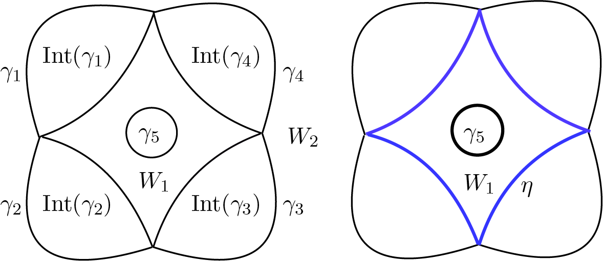
are mutually disjoint (see Figure 4).


Note that when we are saying that the curves
 $\gamma _1,\ldots ,\gamma _n$
are independent, their interior part
 $\mathrm {Int}(\gamma _k)$
is determined. The other component of
 $\widehat {\mathbb {C}}\setminus \gamma _k$
is the exterior part of
 $\gamma _k$
, denoted by
 $\mathrm {Ext}(\gamma _k)$
. Let
 $$ \begin{align*}A(\gamma_1,\ldots,\gamma_n)=\bigcap_{1\leq k\leq n}\mathrm{Ext}(\gamma_k)=\widehat{\mathbb{C}}-\bigcup_{1\leq k\leq n}\overline{\mathrm{Int}(\gamma_k)}.\end{align*} $$
Clearly
 $A(\gamma _1,\ldots ,\gamma _n)$
is an open set and has finitely many connected components. It is worth observing that for any component W of
 $A(\gamma _1,\ldots ,\gamma _n)$
, which is not a Jordan disk, there are independent Jordan curves
 $\eta _1,\ldots ,\eta _m$
for some
 $m\geq 2$
such that
 $W=A(\eta _1,\ldots ,\eta _m)$
, see Figure 4.
An example of independent Jordan curves
 $\gamma _1,\ldots , \gamma _5$
(a), here
 $A(\gamma _1,\ldots ,\gamma _5)=W_1\cup W_2$
, and
 $W_1$
can be written as
 $A(\gamma _5, \eta )$
, where
 $\gamma _5,\eta $
are independent (b).

Proposition 3.4. Let g be a rational map with
 $\infty $
a repelling fixed point. Let
 $\gamma _1, \ldots ,\gamma _n$
be independent Jordan curves in
 $\widehat {\mathbb {C}}$
satisfying:
-
(a)
$\gamma _i\cap \gamma _j=\{\infty \}$
for any
$i\neq j$
; -
(b) all fixed points of g in
$\mathbb {C}$
are contained in
$\mathrm {Int}(\gamma _1)\cup \cdots \cup \mathrm {Int}(\gamma _n)$
; -
(c) in a neighborhood
$N(\infty )$
of
$\infty $
, one has
$$ \begin{align*}N(\infty)\cap \gamma_k\subseteq g(N(\infty)\cap\gamma_k),\quad\text{for all } \ 1\leq k\leq n;\end{align*} $$
-
(d) the unbounded component of
$g^{-1}(\gamma _k)$
is contained in
$\overline {\mathrm {Ext}}(\gamma _k)$
.


Then the unbounded component
 $U_k$
of
 $g^{-1}(\mathrm {Ext}(\gamma _k))$
satisfies
 $$ \begin{align*}U_k\subseteq \mathrm{Ext}(\gamma_k).\end{align*} $$
Further, let
 $\widehat {U}_k$
be the filled closure of
 $U_k$
with respect to
 $\mathrm {Ext}(\gamma _k)$
and let
 $\gamma _k^{-1}=\partial \widehat {U}_k$
. Then:
-
(1)
$\gamma _1^{-1},\ldots ,\gamma _n^{-1}$
are independent Jordan curves with
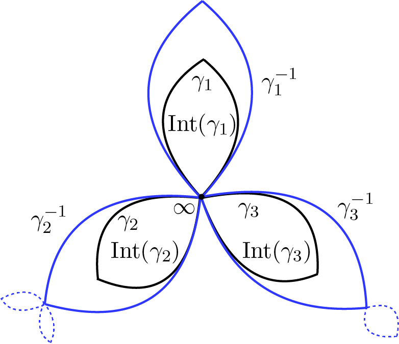
$\overline {\mathrm {Ext}}(\gamma _k^{-1})=\widehat {U}_k$
(see Figure 5); -
(2) in each
$\widehat {U}_k$
, the number of poles (counting multiplicity, see Remark 3.3) equals that of fixed points; -
(3)
$g^{-1}(\mathrm {Ext}(\gamma _k))$
is disjoint from
$\mathrm {Ext}(\gamma _k)\setminus \mathrm {Ext}(\gamma _k^{-1})$
; -
(4) the unbounded component of
$g^{-1}(\overline {A(\gamma _1,\ldots ,\gamma _n)})$
is contained in
$$ \begin{align*}\overline{A(\gamma_1^{-1},\ldots,\gamma_n^{-1})}.\end{align*} $$


Inverse images of independent curves.

Proof. Let
 $\alpha _k$
be the unbounded component of
 $g^{-1}(\gamma _k)$
. The set
 $\alpha _k$
is a union of finitely many Jordan curves, touching at finitely many points. Clearly,
 $\widehat {\mathbb {C}}\setminus \alpha _k$
has finitely many components, and each component of
 $g^{-1}(\mathrm {Ext}(\gamma _k))$
(respectively
 $g^{-1}(\mathrm {Int}(\gamma _k))$
) is contained in one of them. Write
 $$ \begin{align*} \mathrm{Comp} (\widehat{\mathbb{C}}\setminus {\alpha_{k}})= \{C_{k,\infty},C_{k,1},\ldots,C_{k,l},C^{\prime}_{k,\infty}, C^{\prime}_{k,1}, \ldots,C_{k,l^{\prime}}^{\prime} \}, \end{align*} $$
where the notation is labeled so that:
-
(i)
$C_{k,\infty },C_{k,\infty '}$
are the only two unbounded components; -
(ii) each
$C\in \{C_{k,\infty }, C_{k,1},\ldots , C_{k,l}\}$
(respectively
$\{C^{\prime }_{k,\infty }, C^{\prime }_{k,1},\ldots , C^{\prime }_{k,l'}\}$
) contains a component V of
$g^{-1}(\mathrm {Ext}(\gamma _k))$
(respectively
$g^{-1}(\mathrm {Int}(\gamma _k))$
) such that
$\partial C\subseteq \partial V$
.


The unbounded component
 $U_k$
of
 $g^{-1}(\mathrm {Ext}(\gamma _k))$
is contained in
 $C_{k,\infty }$
. By condition (d), either
 $C_{k,\infty }\subseteq \mathrm {Ext}(\gamma _k)$
or
 $\mathrm {Int}(\gamma _k) \subseteq C_{k,\infty }$
. The latter cannot happen, because locally near
 $\infty $
, g behaves like
 $N(\infty )\cap \gamma _k\subseteq g(N(\infty )\cap \gamma _k)$
, and globally, g is orientation preserving. Thus
 $U_k\subseteq C_{k,\infty }\subseteq \mathrm {Ext}(\gamma _k)$
.
We will prove the properties (1)–(4), based on the following claim.
 $$ \begin{align*}\ C_{k,1}\cup\cdots\cup C_{k,l}\subseteq\widehat{U}_k.\end{align*} $$
In fact, if the claim is not true, we have
 $C_{k,i}\subseteq \widehat {\mathbb {C}}\setminus \widehat {U}_k$
for some i. By condition (d), the filled closure
 $\widehat {C}_{k,i}$
of
 $C_{k,i}$
with respect to
 $\widehat {\mathbb {C}}\setminus \widehat {U}_k$
is disjoint from
 $\mathrm {Int}(\gamma _k)$
, and
 $\mathrm {Int}(\gamma _k)\subseteq C_{k,\infty }'$
. Let
 $D=\mathrm {Ext}(\gamma _k)$
and U be a component of
 $g^{-1}(\mathrm {Ext}(\gamma _k))$
contained in
 $C_{k,i}$
. Clearly
 $U\subseteq D$
. Applying Corollary 3.2 to the pair
 $(D, U)$
, we have that
 $\widehat {C}_{k,i}$
contains at least one fixed point of g. This contradicts condition (b), which completes the proof of the claim.
-
(1) The following observation
implies that
$$ \begin{align*}\gamma_i^{-1}\cap\gamma_j^{-1}\subseteq g^{-1}(\gamma_i)\cap g^{-1}(\gamma_j)\subseteq g^{-1}(\gamma_i\cap\gamma_j)=g^{-1}(\infty),\quad i\neq j\end{align*} $$
$\gamma _i^{-1}\cap \gamma _j^{-1}$
is a finite set, as it consists of finitely many poles.
Note that
$\gamma _i\subseteq \overline {\mathrm {Ext}}(\gamma _k)$
for
$i\neq k$
, the unbounded component
$\alpha _i$
of
$g^{-1}(\gamma _i)$
is contained in the unbounded component of
$g^{-1}(\overline {\mathrm {Ext}}(\gamma _k))$
. Therefore,
$\gamma _i^{-1}\subseteq \alpha _i\subseteq \widehat {U}_k$
, and there are mutually disjoint interior parts
${\mathrm {Int}}(\gamma _k^{-1})$
of the curves
$\gamma _k^{-1}$
. This verifies that the curves
$\gamma _k^{-1}$
are independent. -
(2) It is an immediate consequence of Corollary 3.2.
-
(3) It follows from the claim above.
-
(4) Because
the unbounded component of
$$ \begin{align*}\overline{A(\gamma_1,\ldots,\gamma_n)}\subseteq \overline{\mathrm{Ext}}(\gamma_i)\quad\mathrm{for\,\, }1\leq i\leq n,\end{align*} $$
$g^{-1}(\overline {A(\gamma _1,\ldots ,\gamma _n)})$
, denoted by E, is contained in that of
$g^{-1}(\overline {\mathrm {Ext}}(\gamma _i))$
, and therefore
$E\subseteq \widehat {U}_i$
by the claim above. Thus
$E\subseteq \widehat {U}_1\cap \cdots \cap \widehat {U}_n=\overline {A(\gamma _1^{-1},\ldots ,\gamma _n^{-1})}$
.


Proposition 3.5. Let g be a rational map with
 $\infty $
a repelling fixed point. Let
 $\gamma _1, \ldots ,\gamma _n$
be independent Jordan curves in
 $\widehat {\mathbb {C}}$
such that:
-
(1)
$\infty \in \gamma _1\cap \cdots \cap \gamma _n$
; -
(2) all fixed points of g in
$\mathbb {C}$
are contained in
$\mathrm {Int}(\gamma _1)\cup \cdots \cup \mathrm {Int}(\gamma _n)$
; -
(3) in each
$\overline {\mathrm {Ext}}(\gamma _k)\setminus \{\infty \}$
, the number of poles equals that of fixed points.Then the number of poles in
$\overline {A(\gamma _1,\ldots ,\gamma _n)}$
is
$n-1$
, strictly less than n.


Here, the number of poles is counted with multiplicity (see Remark 3.3).
Proof. Let
 $a_k$
(respectively
 $b_k$
) be the number of poles (respectively fixed points) in
 $\overline {\mathrm {Ext}}(\gamma _k)\setminus \{\infty \}$
. Let
 $\widetilde {a}_k$
(respectively
 $\widetilde {b}_k$
) be the number of poles (respectively fixed points) in
 $\mathrm {Int}(\gamma _k)=\widehat {\mathbb {C}}-\overline {\mathrm {Ext}}(\gamma _k)$
. Let a be the number of poles in
 $\overline {H}\setminus \{\infty \}$
, where
 $H=A(\gamma _1,\ldots ,\gamma _n)$
. All these numbers are counted with multiplicities.
The independent curves
 $\gamma _1,\ldots ,\gamma _n$
decompose
 $\mathbb C$
into several parts. These parts satisfy the following relations:
-
(1)
$\overline {\mathrm {Ext}}(\gamma _k)\setminus \{\infty \} =(\overline {H}\setminus \{\infty \})\cup \bigcup _{i\neq k}\mathrm {Int}(\gamma _i)$
; -
(2)
$\mathbb {C}=(\overline {H}\setminus \{\infty \})\cup \bigcup _{1\leq i\leq n}\mathrm {Int}(\gamma _1)$
.


By counting the number of poles, we have the following identity:
 $$ \begin{align*} \sum_{1\leq k\leq n} a_k&= \sum_{1\leq k\leq n}\bigg(a+\sum_{i\neq k}\widetilde{a}_i\bigg)=an+(n-1)\sum_{1\leq i\leq n}\widetilde{a}_i\\ &= a+(n-1)\bigg(a+\sum_{1\leq i\leq n}\widetilde{a}_i\bigg)=a+(n-1)(d-1), \end{align*} $$
where d is the degree of g. Note that
 $\overline {H}\setminus \{\infty \}$
is disjoint from the fixed points of g. By counting the number of fixed points in
 $\mathbb C$
, we have
 $$ \begin{align*}\sum_{1\leq k\leq n} b_k=\sum_{1\leq k\leq n}\bigg(0+\sum_{i\neq k}\widetilde{b}_i\bigg)=(n-1)\sum_{1\leq i\leq n}\widetilde{b}_i=(n-1)d.\end{align*} $$
By assumption, one has
 $a_k=b_k$
for all k, which implies that
 $\sum a_k=\sum b_k$
. Therefore, we have
 $a=n-1$
. The proof is completed.
4 Invariant graph
Let f be a Newton map of degree
 $d\geq 3$
, post-critically finite on
 $ B_f$
. The aim of this section is to prove the existence of an invariant graph for f. Here, a graph G is said to be invariant for f if it satisfies
 $$ \begin{align*}f(G)\subseteq G\quad \text{and}\quad f^{-1}(G) \text{ is connected}.\end{align*} $$
In fact, the existence of an invariant graph is first proven by Drach et al [Reference Drach, Mikulich, Rückert and SchleicherDMRS] and Mikulich, Rückert, and Schleicher [Reference Mikulich, Rückert and SchleicherMRS]. Our work is distinguished from theirs in two aspects.
First, our idea of proof is essentially different from theirs. The construction in Theorem 4.1 is actually inspired by a previous work [Reference Cui, Gao and ZengCGZ]. Analogous to [Reference Cui, Gao and ZengCGZ, Proposition 4.4], it is crucial to see that the point
 $\infty $
(respectively each periodic Fatou center in [Reference Cui, Gao and ZengCGZ]) has to be a non-cut point for the graph that is used to construct puzzles in §5 (respectively tiles in [Reference Cui, Gao and ZengCGZ, §5]). This point is the main goal of our construction. In contrast, the proof in [Reference Drach, Mikulich, Rückert and SchleicherDMRS] aims to show that all the poles lie in the unbounded component, say
 $\Delta _n$
, of
 $f^{-n}(\Delta _0)$
for sufficiently large n; see (4.1) for the definition of channel graph
 $\Delta _0$
. Additionally, it seems to be not clear from [Reference Drach, Mikulich, Rückert and SchleicherDMRS] whether
 $\infty $
is a cut point of
 $\Delta _n$
or not.
Second, our graph is different from theirs. The graph G constructed in Theorem 4.1 is a strict subset of
 $\Delta _n$
. It has very good properties: points in G except some strictly pre-periodic Fatou centers are non-cut points; see Proposition 4.8. Therefore, it is well adapted to construct puzzles; see §5.1. In contrast, for the graph
 $\Delta _n$
, many iterated preimages of
 $\infty $
are cut points. That is the reason why we develop a different proof and construct a different graph.
4.1 Channel graph
For any immediate root basin B of f, there are exactly
 $d_B-1$
fixed internal rays in B:
 $$ \begin{align*}R_{B}({j}/{(d_B-1)}),\quad 0\leq j\leq d_B-2 \text{ where } d_B=\mathrm{deg}(f|_{B}).\end{align*} $$
Each of these fixed internal rays must land at a fixed point on
 $\partial B$
. Because
 $\infty $
is the unique fixed point of f on its Julia set, all fixed internal rays land at the common point
 $\infty $
.
The channel graph of f, denoted by
 $\Delta _0$
, is defined by
 $$ \begin{align} \Delta_0=\bigcup_{B}\bigcup_{j=1}^{d_B-1}\overline{ R_{B}({j}/(d_B-1))}, \end{align} $$
where B ranges over all immediate root basins in
 $\{B_1,\ldots , B_d\}$
. Clearly
 $f(\Delta _0)=\Delta _0$
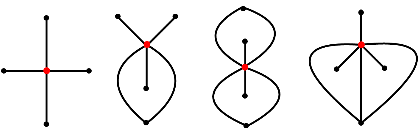
. Figure 6 illustrates all possible channel graphs when
 $d=4$
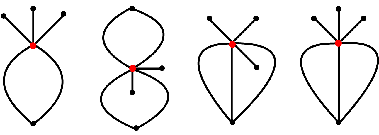
. Some graphs which look like channel graphs but in fact are fake ones are given in Figure 7.
4.2 Invariant graph
The main result in this section is the following.
Theorem 4.1. Let f be a Newton map which is post-critically finite on
 $ B_f$
. Then there exists an invariant graph G such that:
-
(1)
$ f^N(G)=\Delta _0$
for some integer
$N\geq 1$
; -
(2)
$\infty $
is a non-cut point with respect to G.


The idea of the proof. Let us sketch the idea, so that the readers can have a rough picture of the proof. For each
 $k\geq 1$
, let
 $\mathcal C_k=f^{-k}(\Delta _0)\setminus f^{-k+1}(\Delta _0)$
. From Theorem 4.1(1), one may easily imagine that G is actually a union of some suitable iterated preimages of
 $\Delta _0$
.
All possible channel graphs when
 $d=4$
. The red dot is
 $\infty $
and the black dots are the centers of immediate root basins.

Caution: these graphs are not channel graphs for
 $d=4$
, they are fake ones. Want to know why? See Fact 4.2.

These iterated preimages are chosen in an inductive fashion. First, we extend the graph
 $\widetilde {\Delta }_0:=\Delta _0$
to a larger one
 $\widetilde {\Delta }_1$
, by adding a suitable subset of
 $\mathcal C_1$
. Inductively, at step k, we will get an extension of the graph
 $\widetilde {\Delta }_k$
from
 $\widetilde {\Delta }_{k-1}$
by adding a subset of
 $\mathcal C_1\cup \cdots \cup \mathcal C_k$
.
The choice of the subset of
 $\mathcal C_1\cup \cdots \cup \mathcal C_k$
is delicate, we actually choose a suitable subset such that either its endpoint is a pole, or some endpoint of the iterated preimage is a pole. This dichotomy is guaranteed by the shrinking lemma (see Lemma 4.11). The heart of the proof is to show that any subset of this kind can touch another one at some pole. This will be based on the counting number of poles (Propositions 3.4 and 3.5) in the preceding section. However one cannot apply these results directly.
To compensate for the situation, we need to make a modification
 $G_k$
of the graph
 $\widetilde {\Delta }_k$
in each step. For these
 $G_k$
terms, we can apply Propositions 3.4 and 3.5 successfully. For this technical reason, in our discussion, we actually focus on the construction of
 $G_k$
(whose modification yields
 $\widetilde {\Delta }_k$
), and the graphs
 $\widetilde {\Delta }_k$
do not appear directly in the proof.
Then Theorem 4.1(2) can guide each step of the proof. To construct a graph G so that
 $\infty $
is a non-cut point, we construct a sequence of modified graphs
 $G_k$
so that
 $$ \begin{align*}\infty\in G_0\subseteq G_1\subseteq G_2\subseteq\ldots,\end{align*} $$
here, the graph
 $G_0$
is a modified version of the channel graph
 $\Delta _0$
, and
 $G_{k+1}$
is constructed inductively so that the difference set
 $G_{k+1}\setminus G_k$
is the union of finitely many Jordan arcs, and that
 $$ \begin{align*}\nu(G_{k+1}, \infty) < \nu(G_k, \infty)\quad\text{if } \ \nu(G_k, \infty)\geq 2.\end{align*} $$
The property
 $d=\nu (G_0, \infty )>\nu (G_1, \infty )>\nu (G_2, \infty )> \ldots $
implies that after finitely many steps, the procedure will terminate at a graph
 $G_{\ell }$
with
 $\nu (G_{\ell }, \infty )=1$
, which is equivalent to say that
 $\infty $
is a non-cut point for
 $G_{\ell }$
. Finally, a suitable modification of
 $G_{\ell }$
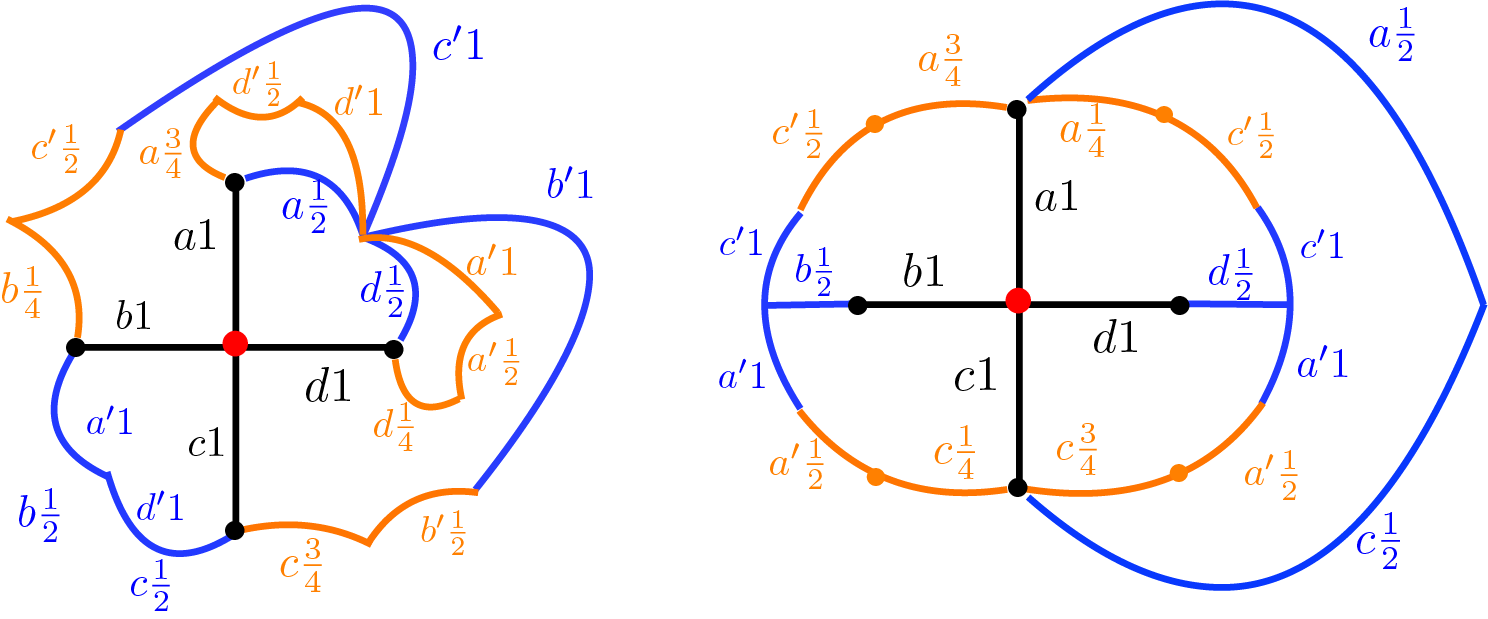
yields the required graph G. See Figures 8 and 9.
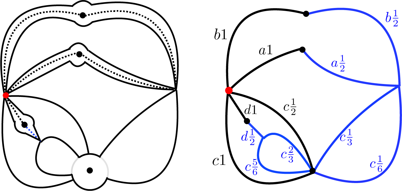
A type of channel graph
 $\Delta _0$
(a) and its resulting invariant graph G (b). Here the red dots represent the same point
 $\infty $
. The notation ‘
 $w t$
’ means the internal ray of angle t starting from the center
 $w\in \{a,b,c,d\}$
.

Two invariant graphs for two different maps. Their channel graphs are the same, but the combinations are different. The notation ‘
 $w t$
’ means the internal ray of angle t starting from the center
 $w\in \{a,b,c,d\}\cup \{a',b',c',d'\}$
, here
 $x'$
is a preimage of x. The blue/orange parts are the subsets of the first/second preimages of the channel graph.

Proof of Theorem 4.1
The proof proceeds in six steps, as follows.
Step 1: from
 $\Delta _0$
to
 $G_0$
. The aim of this step is to modify
 $\Delta _0$
to a new graph
 $G_0$
, such that
 $G_0$
is disjoint from the d attracting fixed points.
Consider an immediate root basin B of f. Recall that
 $\Phi _B:B\to \mathbb {D}$
is a Böttcher map, satisfying that
 $\Phi _B(z)^{d_B}=\Phi _B(f(z))$
. Fix a number
 $r\in (0,1)$
.
If
 $d_B\geq 3$
, let
 $$ \begin{align*}\Delta_B=\{\infty\}\cup \Phi_B^{-1}(\{[r,1) e^{2\pi i k/(d_B-1)}; 0\leq k\leq d_B-2\})\cup\Phi_B^{-1}(r\mathbb S).\end{align*} $$
If
 $d_B=2$
, take a small angle
 $\theta _0\in (0,1/2)$
and define two arcs
 $\alpha _{\pm }$
in B by
 $$ \begin{align*}\alpha_{\pm}=\Phi_B^{-1}(\{e^{s(\log r\pm 2\pi i\theta_0)}; 0<s<1\}).\end{align*} $$
Clearly,
 $\alpha _{\pm }$
connect
 $\infty $
to
 $\Phi _B^{-1}(re^{\pm 2\pi i \theta _0})$
, and
 $\alpha _{\pm }\subseteq f(\alpha _{\pm })$
. For convenience, in this case, we say that the arcs
 $\alpha _{\pm }$
are tangent to the internal ray
 $\Phi _B^{-1}((0,1))$
at
 $\infty $
. The preimages
 $f^{-n}(\alpha _{\pm })$
are also said to be tangent to internal rays
 $f^{-n}(\Phi _B^{-1}((0,1)))$
at some points in
 $f^{-n}(\infty )$
. We set
 $$ \begin{align*}\Delta_B=\{\infty\}\cup\alpha_+\cup\alpha_-\cup \Phi_B^{-1}(\{r\,e^{2\pi i t};\ \theta_0\leq t\leq -\theta_0\}).\end{align*} $$
Finally, let
 $$ \begin{align*}G_0=\bigcup_{B}\Delta_B,\end{align*} $$
where the union is taken over all immediate root basins B of f. Clearly
 $G_0$
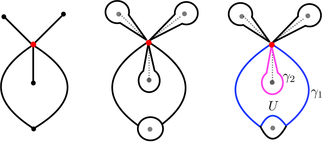
avoids all centers of the immediate root basins. See Figure 10.
The channel graph
 $\Delta _0$
(a), the modified graph
 $G_0$
(b), and a non-trivial component U of
 $\widehat {\mathbb {C}}\setminus G_0$
(c). This U can be written as
 $A(\gamma _1, \gamma _2)$
, where
 $\gamma _1$
is the blue curve and
 $\gamma _2$
is the purple one.

Step 2: from
 $G_0$
to
 $G_1$
. For a finite graph
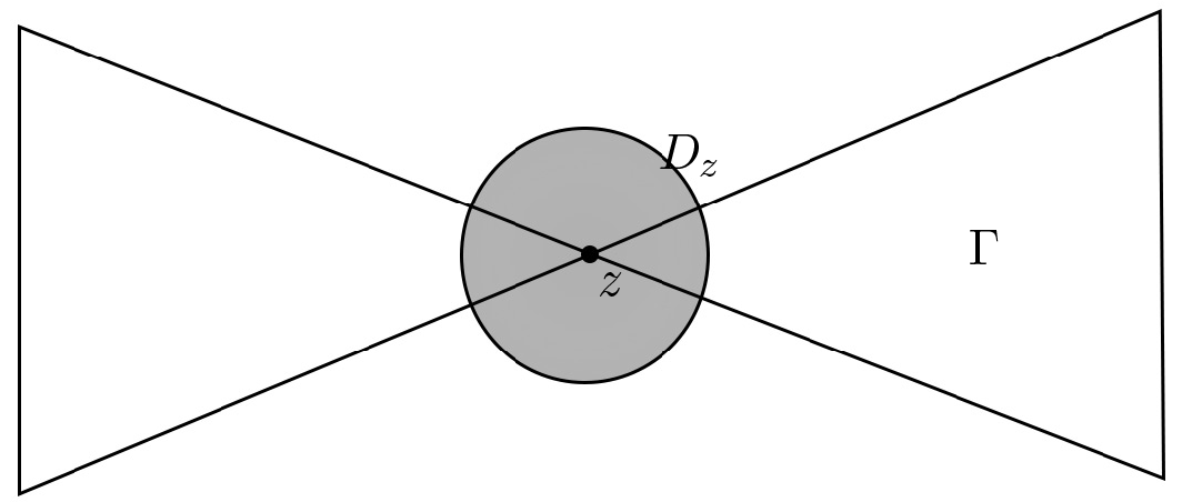
 $\Gamma \subseteq \widehat {\mathbb {C}}$
with
 $\infty \in \Gamma $
, its complement
 $\widehat {\mathbb {C}}\setminus \Gamma $
has finitely many components. There are two kinds of unbounded ones. An unbounded component U of
 $\widehat {\mathbb {C}}\setminus \Gamma $
is called trivial if
 $\nu (\partial U, \infty )=1$
(equivalently,
 $\infty $
is a non-cut point of
 $\partial U$
); non-trivial if
 $\nu (\partial U, \infty )\geq 2$
(i.e.,
 $\infty $
is a cut point of
 $\partial U$
).
For the graph
 $G_0$
given by Step 1, the following fact is non-trivial.
Fact 4.2. An unbounded component U of
 $\widehat {\mathbb {C}}\setminus G_0$
is trivial (that is,
 $\partial U\setminus \{\infty \}$
is connected) if and only if
 $\partial U=\Delta _B$
with
 $d_B=2$
.
Proof. The ‘
 $\Longleftarrow $
’ part is obvious. We need to show the ‘
 $\Longrightarrow $
’ part. If it is not true, then there are two possibilities for U:
-
(1)
$\partial U$
intersects at least two root basins; or -
(2)
$\partial U$
is a component of
$\widehat {\mathbb {C}}-\Delta _B$
with
$d_B\geq 3$
(see Figures 10 and 11).


The former case implies that
 $\partial U\setminus \{\infty \}$
has at least two components. Hence it is impossible.
In the following, we consider the latter case. Note that
 $U\subseteq f(U)$
and the image
 $f(U\cap B)$
covers
 $U\cap B$
twice. One may also observe that there is a component V of
 $f^{-1}(U)$
, contained in U, such that
 $\partial V$
contains two sections of fixed internal rays. Note that
 $\overline {V}$
contains only one fixed point, namely
 $\infty $
. However, by Lemma 3.1, one has
 $$ \begin{align*}\#\mathrm{Fix}(f|_{\overline{V}})=\mathrm{deg}(f|_{\partial V}).\end{align*} $$
This gives a contradiction, because
 $\#\mathrm {Fix}(f|_{\overline {V}})=1$
and
 $\mathrm {deg}(f|_{\partial V})\geq 2$
.
Fact 4.2 has the following interesting corollary.
Fact 4.3. Under the assumption
 $d=\mathrm {deg}(f)\geq 3$
, there are at least two immediate root basins B with
 $d_B=2$
. As a consequence, trivial and non-trivial components both exist in
 $\mathrm {Comp}(\widehat {\mathbb {C}}\setminus G_0)$
.


Proof. This fact is obvious if
 $d_B=2$
for all immediate root basins B. So we may assume
 $d_B\geq 3$
for some B. In this case,
 $\widehat {\mathbb {C}}-\Delta _B$
has at
 $d_B-1\geq 2$
unbounded components. To prove the fact, we will show each unbounded component of
 $\widehat {\mathbb {C}}-\Delta _B$
contains an immediate root basin
 $B''$
with
 $d_{B''}=2$
.
In fact, if some unbounded component of
 $\widehat {\mathbb {C}}-\Delta _B$
, say U, contains no immediate root basin
 $B'$
with
 $d_{B'}=2$
, then there are two cases:
-
(1) there is no immediate root basin completely contained in U; or
-
(2) all immediate root basins
$B''$
in U satisfy that
$d_{B''}\geq 3$
.


In the former case, U is trivial. However, this contradicts Fact 4.2.
In the latter case, we can find an immediate root basin
 $B''\subseteq U$
, which is an innermost one, and such that some unbounded component V of
 $\widehat {\mathbb {C}}-\Delta _{B''}$
is also trivial (this is an easy observation). This again contradicts Fact 4.2.
The idea of this step is to take pullbacks of the boundaries of non-trivial unbounded components of
 $\widehat {\mathbb {C}}\setminus G_0$
.
Let
 $Q_0$
be a non-trivial unbounded component of
 $\widehat {\mathbb {C}}\setminus G_0$
. Such a component can be written as
 $Q_0=A(\gamma _1,\ldots ,\gamma _n)$
where
 $n\geq 2$
and
 $\gamma _1,\ldots ,\gamma _n$
are independent Jordan curves. One may verify that the curves
 $\gamma _1,\ldots ,\gamma _n$
satisfy the conditions (a)–(d) in Proposition 3.4. Indeed, by the construction in Step 1, the conditions (a)–(c) are satisfied, we only need to check that the unbounded component
 $\alpha _k$
of
 $f^{-1}(\gamma _k)$
is contained in
 $\overline {\mathrm {Ext}}(\gamma _k)$
. To see this, note that either
 $\alpha _k\subseteq \overline {\mathrm {Int}}(\gamma _k)$
or
 $\alpha _k\subseteq \overline {\mathrm {Ext}}(\gamma _k)$
; the former cannot happen, the reason is that
 $\gamma _k$
contains a section of some equipotential curve
 $\Phi _B^{-1}(r\partial \mathbb D)$
(for some immediate root basin B) and
 $\alpha _k$
contains a section of the equipotential curve
 $\Phi _B^{-1}(\sqrt [d_B\,\,\,\,]{r}\partial \mathbb D)$
, which can not be completely contained in
 $\overline {\mathrm {Int}}(\gamma _k)$
.
We then apply Proposition 3.4 to the independent curves
 $\gamma _1,\ldots ,\gamma _n$
, and obtain the new independent Jordan curves
 $\gamma _1^{-1},\ldots ,\gamma _n^{-1}$
. For these new curves, observe that:
-
(1) for each k, the curve
$\gamma _k^{-1}$
contains at least one pole of f in
$\mathbb {C}$
; -
(2) one has
$\gamma _i^{-1}\cap \gamma _j^{-1}\subseteq f^{-1}(\infty )$
, for
$i\neq j$
.


In the following, we will show that at least two curves of
 $\gamma _1^{-1},\ldots ,\gamma _n^{-1}$
have a common pole. In fact, if this is not true, then the set
 $\overline {A(\gamma _1^{-1},\ldots ,\gamma _n^{-1})}$
contains at least n distinct poles. However, by Proposition 3.4, the curves
 $\gamma _1^{-1},\ldots ,\gamma _n^{-1}$
satisfy the assumptions in Proposition 3.5. Then by Proposition 3.5, the number of poles in
 $\overline {A(\gamma _1^{-1},\ldots ,\gamma _n^{-1})}$
is exactly
 $n-1$
(counting multiplicity). This is a contradiction.
Finally, let us define three curve families
 $\Gamma _0, \Gamma ^*_1, \Gamma _1$
, and a new graph
 $G_1$
by
 $$ \begin{align*}\Gamma_0=\bigcup_{Q_0}\{\gamma_1,\ldots,\gamma_n\},\ \Gamma^*_1=\Gamma_1=\bigcup_{Q_0}\{\gamma_1^{-1},\ldots,\gamma_n^{-1}\},\ G_1=\bigcup_{\gamma\in \Gamma^*_1}\gamma,\end{align*} $$
where
 $Q_0$
ranges over all non-trivial unbounded components of
 $\widehat {\mathbb {C}}\setminus G_0$
. The existence of common poles for the curves
 $\gamma _k^{-1}$
, implies that
 $$ \begin{align*}\nu(G_1,\infty)<\nu(G_0,\infty)=d.\end{align*} $$
Note that we have the inclusion
 $$ \begin{align*}f(\Gamma_1):=\{f(\gamma);\gamma\in\Gamma_1\}\subseteq \Gamma_0, \ \ f(G_1)\subseteq G_0.\end{align*} $$
Step 3: from
 $G_1$
to
 $G_2$
. The idea of the proof is similar to that of Step 2: taking pullbacks of the boundaries of non-trivial unbounded components of
 $\widehat {\mathbb {C}}\setminus G_1$
, until some pullback hits a pole. We remark that this step actually reveals the general case of the pullback procedure. The shrinking lemma is involved to deal with the difficulty arising here.
Note that if
 $\nu (G_1,\infty )=1$
, then
 $\infty $
is a non-cut point of
 $G_1$
, and hence there is nothing to do in this step. So we may assume that
 $\nu (G_1,\infty )\geq 2$
, and this case happens if and only if there exists a non-trivial unbounded component, say
 $Q_1$
, of
 $\widehat {\mathbb {C}}\setminus G_1$
.
Note that
 $Q_1$
is contained in some
 $Q_0=A(\gamma _1,\ldots ,\gamma _n)$
in Step 2, and that
 $Q_0$
is decomposed by the curves
 $\gamma ^{-1}_1,\ldots ,\gamma _n^{-1}$
into several parts. Because
 $Q_1$
is non-trivial, it can be written as
 $$ \begin{align*}Q_1=A(\alpha_1,\ldots,\alpha_m),\end{align*} $$
where
 $\alpha _1,\ldots ,\alpha _m$
are independent Jordan curves. The set
 $\{\alpha _1,\ldots ,\alpha _m\}$
can be decomposed into two disjoint subsets
 $\Gamma _1(Q_1)$
and
 $\Xi (Q_1)$
, such that:
-
(1) each curve
$\lambda \in \Gamma _1(Q_1)$
comes from
$\Gamma _1$
, namely
$\Gamma _1(Q_1)\subseteq \Gamma _1$
; -
(2) each curve
$\eta \in \Xi (Q_1)$
is new, that is, composed of several sections, each section is a part of a curve in
$\Gamma _1$
.


Note that each curve
 $\lambda \in \Gamma _1(Q_1)\subseteq \Gamma _1$
must contain a pole in
 $\mathbb {C}$
. Each curve
 $\eta \in \Xi (Q_1)$
must also contain a pole in
 $\mathbb {C}$
, because if two curves in
 $\Gamma _1$
intersect at a point other than
 $\infty $
, then this point is a pole.
Fact 4.4.
 $\Xi (Q_1)\neq \emptyset $
. In other words, at least one curve among
 $\alpha _k$
is new.
Proof. If not, then
 $\Gamma _1(Q_1)=\{\alpha _1,\ldots ,\alpha _m\}\subseteq \Gamma _1$
, and
 $\alpha _i\cap \alpha _j=\{\infty \}$
for
 $i\neq j$
. Therefore, the number of poles in
 $\overline {Q}_1=\overline {A(\alpha _1,\ldots ,\alpha _m)}$
is at least m.
However, applying Proposition 3.4 to the curves
 $f(\alpha _1), \ldots , f(\alpha _m)$
, we see that the curves
 $\alpha _1,\ldots ,\alpha _m$
satisfy the assumptions in Proposition 3.5. Then by Proposition 3.5, the number of poles in
 $\overline {A(\alpha _1,\ldots ,\alpha _m)}$
is exactly
 $m-1$
(counting multiplicity). This is a contradiction.
We may write
 $$ \begin{align*}\Gamma_1(Q_1)=\{\lambda_1,\ldots,\lambda_r\}, \ \Xi(Q_1)=\{\eta_1,\ldots, \eta_s\}.\end{align*} $$
Claim. The Jordan curves
 $f(\lambda _1),\ldots ,f(\lambda _r), \eta _1,\ldots ,\eta _s$
are independent, and satisfy the conditions of Proposition 3.4.
Proof. By the definition of
 $Q_1$
, we see that
 $\lambda _1,\ldots ,\lambda _r, \eta _1,\ldots , \eta _s$
are in different components of
 $\widehat {\mathbb {C}}\setminus Q_1$
. So the bound mutually disjoint components are
 $\mathrm {Int}(\lambda _1),\ldots , \mathrm {Int}(\lambda _r), \mathrm {Int}(\eta _1),\ldots , \mathrm {Int}(\eta _s)$
. Because
 $f(\lambda _k)\subset \overline {\mathrm {Int}}(\lambda _k)$
(we have proven this when we deal with
 $Q_0$
), we see immediately that
 $f(\lambda _1),\ldots ,f(\lambda _r), \eta _1,\ldots ,\eta _s$
are independent, and they satisfy the conditions of Proposition 3.4.
Applying Proposition 3.4 to these curves, for each
 $\eta _j$
, one gets
 $\eta _j^{-1}$
. Moreover, the curves
 $\lambda _1,\ldots ,\lambda _r,\eta ^{-1}_1,\ldots , \eta ^{-1}_s$
are independent.
If one of the resulting curves
 $\eta ^{-1}_j$
, say
 $\eta _k^{-1}$
, is disjoint from poles in
 $\mathbb {C}$
, then it is exactly the unbounded component of
 $f^{-1}(\eta _k)$
, and:
-
(1)
$\eta _k^{-1}$
intersects each of
$\lambda _1,\ldots ,\lambda _r,\eta ^{-1}_j, j\neq k,$
only at
$\infty $
; -
(2)
$f:\eta _k^{-1}\to \eta _k$
is one-to-one.


For any integer
 $l\geq 1$
, one may define
 $\eta _k^{-l-1}$
inductively by
 $$ \begin{align*}\eta_k^{-l-1}=(\eta_k^{-l})^{-1}\end{align*} $$
as long as the curves
 $$ \begin{align*}f(\lambda_1),\ldots,f(\lambda_r),\eta_1,\ldots, \eta_{k-1}, \eta_k^{-l}, \eta_{k+1}, \ldots,\eta_s,\end{align*} $$
are independent, and
 $\eta _k^{-1},\ldots , \eta _k^{-l}$
are disjoint from poles in
 $\mathbb {C}$
. In this case, the curves
 $\lambda _1,\ldots ,\lambda _r,\eta _1^{-1},\ldots , \eta _{k-1}^{-1}, \eta _k^{-l-1},\eta _{k+1}^{-1},\ldots ,\eta _s^{-1}$
are independent.
To continue our discussion, we need the following crucial fact.
Lemma 4.5. For each curve
 $\eta \in \Xi (Q_1)=\{\eta _1,\ldots , \eta _s\}$
, there is a minimal integer
 $N=N_{\eta }\geq 1$
, such that
 $\eta ^{-N}$
contains a pole of f in
 $\mathbb {C}$
.
Proof. If it is not true for
 $\eta =\eta _k$
, then for any
 $j\geq 1$
, the curves
 $\lambda _1,\ldots ,\lambda _r$
,
 $\eta _1^{-1}$
,
 $\ldots , \eta _{k-1}^{-1}, \eta _k^{-j},\eta _{k+1}^{-1},\ldots ,\eta _s^{-1}$
are independent, and the domains
 $$ \begin{align*}H_j=A(\lambda_1,\ldots,\lambda_r,\eta_1^{-1},\ldots, \eta_{k-1}^{-1}, \eta_k^{-j},\eta_{k+1}^{-1},\ldots,\eta_s^{-1})\end{align*} $$
satisfy
 $$ \begin{align*}H_1\supseteq H_2\supseteq \cdots \supseteq H_j\supseteq \cdots.\end{align*} $$
In particular, we have
 $$ \begin{align*}\mathrm{Int}(\eta_k^{-1})\subseteq \mathrm{Int}(\eta_k^{-j}) \quad \text{and}\quad \mathrm{Int}(\lambda_1)\cup\cdots\cup \mathrm{Int}(\lambda_r) \subseteq \mathrm{Ext}(\eta^{-j}_k).\end{align*} $$
This implies that the spherical diameters
 $\mathrm {diam}(\eta _k^{-j})$
with
 $j\geq 1$
are uniformly bounded from below and above.
To get a contradiction, we will show
 $\mathrm {diam}(\eta _k^{-j})\to 0$
as
 $j\to \infty $
. Note that all Jordan curves
 $\eta _k^{-j}$
traverse two distinct immediate root basins, say
 $B', B''$
. We may decompose
 $\eta _k^{-j}$
into three segments
 $\beta _j,\beta ^{\prime }_j, \beta ^{\prime \prime }_j$
:
-
(1)
$\beta _j'$
(respectively
$\beta _j''$
) is the intersection of
$\eta _k^{-j}$
with the closure of some fixed internal ray of
$B'$
(respectively
$B''$
), it takes the form
$\overline {\phi _{B'}^{-1}((r^{1/d_{B'}^j}, 1)e^{2\pi i k/(d_{B'}-1)})}$
for some k; -
(2)
$\beta _j=\eta _k^{-j}\setminus (\beta _j'\cup \beta _j'')$
.


The observation
 $\bigcap _{j} \beta ^{\prime }_j=\bigcap _{j}\beta _j''=\{\infty \}$
implies that
 $\mathrm {diam}(\beta _j')\to 0$
and
 $\mathrm {diam}(\beta _j'')\to 0$
as
 $j\to \infty $
. It remains to prove
 $$ \begin{align*}\mathrm{diam}(\beta_j)\to 0 \quad \mathrm{as}\quad j\to\infty.\end{align*} $$
Note that
 $f:\beta _{j+1}\rightarrow \beta _j$
is a homeomorphism. By the construction of
 $\beta _j$
, there is a large integer
 $n_0>0$
such that
 $\beta _{0}\cap \beta _{n_0}=\emptyset $
. It follows that
 $\beta _{jn_0}\cap \beta _{(j+1)n_0}=\emptyset $
for all
 $j\geq 0$
.
Choose a large integer
 $n_0>0$
such that
 $\beta _{0}\cap \beta _{n_0}=\emptyset $
, and
 $\beta _{n_0}$
has no intersection with the postcritical set. Choose a disk neighborhood
 $U_{0}$
of
 $\overline {\beta _{n_0}}$
such that
 $f^{n_0}(U_{0})\cap U_{0}=\emptyset $
. Then by pulling back
 $U_{0}$
via
 $f^{kn_0}$
, we get a disk neighborhood
 $U_{k}$
of
 $\beta _{kn_0}$
. It follows that there exists a sequence of open sets
 $\{U_j\}$
with
 $\beta _{jn_0}\Subset U_j$
such that
 $f^{n_0}(U_{j+1})=U_j$
and
 $U_{j+1}\cap U_0=\emptyset $
for
 $j\geq 0$
. By the shrinking lemma (see Lemma 4.11), one has
 $\mathrm {diam}(\beta _{jn_0})\to 0$
as
 $j\to \infty $
. The shrinking property
 $H_j\supseteq H_{j+1}$
implies that
 $\mathrm {diam}(\beta _j)\to ~0$
as
 $j\to \infty $
. This gives a contradiction.
Remark 4.6. In Lemma 4.5, it may happen that for some
 $N\geq 1$
,
 $$ \begin{align*}\eta^{-N}\cap f^{-1}(\infty)=\eta\cap f^{-1}(\infty).\end{align*} $$
In other words, the poles in
 $\eta ^{-N}$
are already contained in
 $\eta $
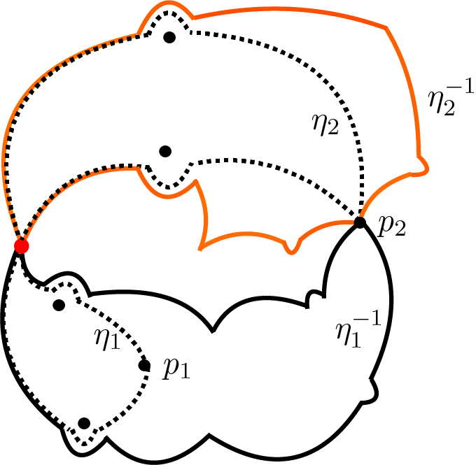
, and hence not new. Figure 12 gives such an example (in this example
 $\eta =\eta _2, N=1$
).
In this example, the black dashed curves
 $\eta _1, \eta _2$
contain the poles
 $p_1, p_2$
, respectively. Here,
 $\eta _1^{-1}$
is the black curve containing the new pole
 $p_2$
, and
 $\eta _2^{-1}$
is the orange curve containing the same pole
 $p_2$
as
 $\eta _2$
does. The pole
 $p_2$
is also a critical point.

By Lemma 4.5, for each
 $\eta _k$
, there exists a minimal integer
 $N_k\geq 1$
such that
 $\eta _k^{-N_k}$
contains a pole. One may verify further that the Jordan curves
 $$ \begin{align*}f(\lambda_1), \ldots, f(\lambda_r),\eta_1^{-l_1},\ldots,\eta_s^{-l_s}\end{align*} $$
with
 $0\leq l_1< N_1,\ldots ,0\leq l_s< N_s$
are independent and satisfy the conditions (a)–(d) in Proposition 3.4. Applying Proposition 3.4 to the curves
 $$ \begin{align*}f(\lambda_1),\ldots,f(\lambda_r),\eta_1^{-N_1+1},\ldots,\eta_s^{-N_s+1},\end{align*} $$
we get the following independent curves
 $$ \begin{align*}\lambda_1,\ldots,\lambda_r,\eta_1^{-N_1},\ldots,\eta_s^{-N_s},\end{align*} $$
each of which contains a pole in
 $\mathbb {C}$
. Again Proposition 3.5 implies that at least two of these curves contain a common pole in
 $\mathbb {C}$
. We remark that each
 $\eta _k$
passes through exactly two immediate root basins
 $B',B''$
, and so do the curves
 $\eta _k^{-j}, 1\leq j\leq N_k$
; these Jordan curves overlap on an invariant subarc in
 $\{\infty \}\cup B'\cup B''$
.
Let us define two families of Jordan curves
 $$ \begin{align*}\Gamma^*_2=\bigcup_{Q_1}\{\eta_1^{-1},\ldots, \eta_1^{-N_1},\ldots,\eta_s^{-1},\ldots, \eta_s^{-N_s}\},\quad \Gamma_2=\bigcup_{Q_1}\{\eta_1^{-N_1},\ldots,\eta_s^{-N_s}\},\end{align*} $$
where
 $Q_1$
ranges over all non-trivial unbounded components of
 $\widehat {\mathbb {C}}\setminus G_1$
. Now we get a new graph
 $G_2$
, which is an extension of
 $G_1$
:
 $$ \begin{align*}G_2=G_1\bigcup \bigcup_{\gamma\in \Gamma^*_2}\gamma.\end{align*} $$
Observe that
 $f(G_2)\subseteq G_0\cup G_2$
. The construction and the existence of common poles for the curves
 $\lambda _1,\ldots ,\lambda _r$
,
 $\eta _1^{-N_1},\ldots ,\eta _s^{-N_s}$
imply that
 $$ \begin{align*}\nu(G_2,\infty)<\nu(G_1,\infty).\end{align*} $$
Step 4: from
 $G_k$
to
 $G_{k+1}$
, an induction procedure. Suppose for some
 $k\geq 2$
, we have constructed the graphs
 $G_1, \ldots , G_k$
and the curve families
 $\Gamma ^*_1, \Gamma _1$
 $\ldots , \Gamma ^*_k, \Gamma _k$
, inductively in the following way:
 $$ \begin{align*}\Gamma^*_l&=\bigcup_{Q_{l-1}}\{\eta_1^{-1},\ldots, \eta_1^{-N_1},\ldots,\eta_s^{-1},\ldots, \eta_s^{-N_s}\},\\[3pt] \Gamma_l&=\bigcup_{Q_{l-1}}\{\eta_1^{-N_1},\ldots,\eta_s^{-N_s}\}, \ G_{l}=G_{l-1}\bigcup \bigcup_{\gamma\in \Gamma^*_l}\gamma, \end{align*} $$
where
 $Q_{l-1}$
is taken over all non-trivial unbounded components of
 $\widehat {\mathbb {C}}\setminus G_{l-1}$
, and that
 $f(G_l)\subseteq G_0\cup G_l$
and
 $\nu (G_l,\infty )<\nu (G_{l-1},\infty )$
, for
 $2\leq l\leq k$
.
If
 $\nu (G_k,\infty )=1$
, then the step is done. If
 $\nu (G_k,\infty )\geq 2$
, we consider each non-trivial unbounded component
 $Q_{k}$
of
 $\widehat {\mathbb {C}}\setminus G_k$
. Write
 $Q_k$
as
 $A(\delta _1,\ldots , \delta _t)$
and compare the curves
 $\delta \in \{\delta _1,\ldots , \delta _t\}$
with the curves in
 $\Gamma _1\cup \cdots \cup \Gamma _k$
, there are two possibilities: either
-
(1)
$\delta \in \Gamma _1\cup \cdots \cup \Gamma _k$
; or -
(2)
$\delta $
is new, that is,
$\delta \notin \Gamma _1\cup \cdots \cup \Gamma _k$
. In this case,
$\delta $
is composed of several sections, and each section is a part of a curve in
$\Gamma _1\cup \cdots \Gamma _k$
.


Let
 $\Xi (Q_k)$
be the collection of new curves. For each
 $\eta \in \Xi (Q_k)$
, by the same argument as Lemma 4.5, there is a minimal integer
 $N_\eta \geq 1$
such that
 $\eta ^{-N_\eta }$
meets a pole in
 $\mathbb {C}$
. By Proposition 3.5, at least two curves of
 $\{\eta ^{-N_\eta }; \eta \in \Xi (Q_k)\}$
share a common pole. Similarly as above, we get a new graph
 $G_{k+1}$
and two curve families
 $\Gamma _{k+1}\subseteq \Gamma _{k+1}^*$
:
 $$ \begin{align*}\Gamma^*_{k+1}=\bigcup_{Q_{k}} \bigcup_{\eta\in \Xi(Q_k)}\{\eta^{-1},\ldots,\eta^{-N_\eta}\}, \quad \Gamma_{k+1}=\bigcup_{Q_{k}} \bigcup_{\eta\in \Xi(Q_k)}\{\eta^{-N_\eta}\},\end{align*} $$
 $$ \begin{align*}G_{k+1}=G_{k}\bigcup \bigcup_{\gamma\in \Gamma^*_{k+1}}\gamma,\end{align*} $$
where
 $Q_{k}$
is taken over all the non-trivial unbounded component
 $Q_{k}$
of
 $\widehat {\mathbb {C}}\setminus G_k$
.
The resulting graph
 $G_{k+1}$
satisfies
 $$ \begin{align*}\nu(G_{k+1},\infty)<\nu(G_k,\infty), \quad f(G_{k+1})\subseteq G_0\cup G_{k+1}.\end{align*} $$
After finitely many steps, we have
 $\nu (G_\ell ,\infty )=1$
for some minimal integer
 $\ell \geq 1$
. Then
 $\infty $
is a non-cut point for the graph
 $G_\ell $
, and
 $f(G_\ell )\subseteq G_0\cup G_\ell $
.
Step 5: from
 $G_\ell $
to G, a natural modification. By construction, all points in
 $G_\ell \cap J(f)$
are iterated preimages of
 $\infty $
, and
 $$ \begin{align*}f(G_\ell\cap J(f))\subseteq G_\ell\cap J(f), \quad f^N(G_\ell\cap J(f))=\{\infty\}\end{align*} $$
for some large integer
 $N\geq 1$
. Note that for any
 $0\leq k\leq \ell $
, the graph
 $G_k$
is a union of some curves in
 $$ \begin{align*}\Gamma=\Gamma_0\cup\Gamma^*_1\cup \Gamma^*_2\cup \Gamma^*_3\cup \cdots\cup \Gamma^*_\ell.\end{align*} $$
To give a natural modification of
 $G_{\ell }$
, it suffices to define the modification of each curve
 $\delta \in \Gamma $
. This goes in the following way.
Let
 $B\in \mathrm {Comp}(B_f)$
with
 $B\cap \delta \neq \emptyset $
, then
 $B\cap \delta $
consists of finitely many components. Suppose B is eventually iterated to the immediate root basin
 $B_0$
. Note that each component
 $\sigma $
of
 $B\cap \delta $
is an open arc, and near the boundary
 $\partial B$
,
 $\sigma $
is either tangent to (if
 $d_{B_0}=2$
) or equal to (if
 $d_{B_0}\geq 3$
) two internal rays (see Figure 13), say
 $R_B(\alpha ), R_B(\beta )$
. We define the modification
 $\mathcal {M}(\sigma )$
of
 $\sigma $
by
 $$ \begin{align*}\mathcal{M}(\sigma)=R_B(\alpha)\cup R_B(\beta)\cup\{c_B\},\end{align*} $$
where
 $c_B$
is the center of B (it is possible that
 $\alpha =\beta $
). We then set
 $$ \begin{align*}\mathcal{M}(\delta)=\overline{\bigcup_B\bigcup_\sigma \mathcal{M}(\sigma)},\end{align*} $$
where B ranges over all components
 $B\in \mathrm {Comp}(B_f)$
with
 $B\cap \delta \neq \emptyset $
and
 $\sigma $
is taken over all components of
 $B\cap \delta $
.
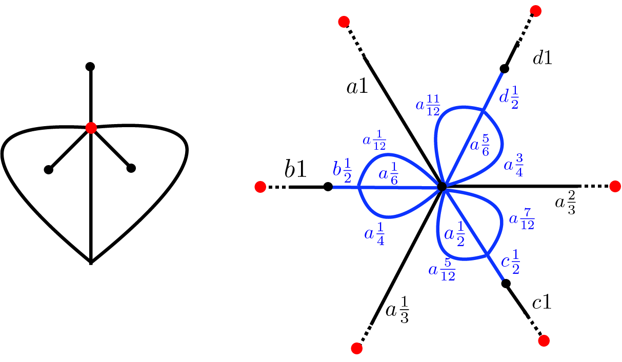
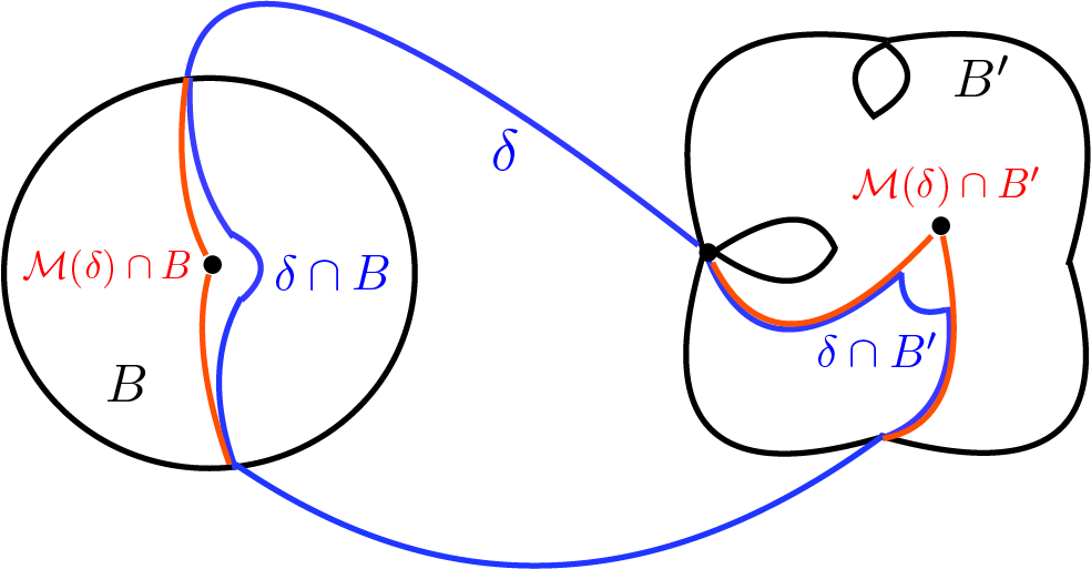
This figure shows how to modify a curve arc by arc. Here,
 $B\cap \delta $
is tangent to two internal rays near
 $\partial B$
, while
 $B'\cap \delta $
is equal to two internal rays near
 $\partial B'$
.

By the law
 $\mathcal M(\delta _1\cup \delta _2)=\mathcal M(\delta _1)\cup \mathcal M(\delta _2)$
, we obtain the modification of the graphs
 $G_k$
, which satisfy
 $$ \begin{align*}\Delta_0=\mathcal{M}(G_0)\subseteq \mathcal{M}(G_1) \subseteq \cdots\subseteq \mathcal{M}(G_\ell)\subseteq f^{-N}(\Delta_0).\end{align*} $$
Let
 $G=\mathcal {M}(G_\ell )$
. Clearly one has
 $f^{N}(G)=\Delta _0$
. Moreover,
 $$ \begin{align*}f(G)=\mathcal{M}(f(G_\ell))\subseteq \mathcal{M}(G_0\cup G_\ell)=\mathcal{M}(G_\ell)=G.\end{align*} $$
 $$ \begin{align*}\nu(G,\infty)=\nu(G_\ell,\infty)=1.\end{align*} $$
(See Figure 14.)
Step 6:
 $f^{-1}(G)$
is connected. To prove the connectivity of
 $f^{-1}(G)$
, we need to investigate some properties of G and
 $G_\ell $
(given in Step 4) first.
Fact 4.7. Each component of
 $\widehat {\mathbb {C}}\setminus G_\ell $
is a Jordan disk.
Proof. It is equivalent to show that
 $\nu (G_\ell , z)=1$
for all
 $z\in G_{\ell }$
. Clearly this is true for
 $z=\infty $
by the construction of
 $G_\ell $
. For
 $z\in G_{\ell }-\{\infty \}$
, note that
 $G_\ell =\bigcup _{\delta \in \Gamma \setminus \Gamma _0}\delta $
(here
 $\Gamma ,\Gamma _0$
are defined in Step 5) and
 $\infty \in \bigcap _{\delta \in \Gamma \setminus \Gamma _0}\delta $
. The observation
 $G_{\ell }\setminus \{z\}= \bigcup _{\delta \in \Gamma \setminus \Gamma _0}(\delta \setminus \{z\})$
and
 $\infty \in \bigcap _{\delta \in \Gamma \setminus \Gamma _0}(\delta \setminus \{z\})$
imply that
 $G_{\ell }\setminus \{z\}$
is connected, and hence z is not a cut point of
 $G_\ell $
.
Proposition 4.8. The graph G satisfies:
-
(1) any point in
$G\cap J(f)$
is not a cut point of G; -
(2) the center of any immediate root basin is a non-cut point of G;
-
(3) for any immediate root basin B, the intersection
$G\cap \overline {B}$
is connected. In other words, any Julia point in
$\overline {B}\cap J(f)$
is linked to the center of B by an internal ray in G.


This figure shows how to get the graph G (a) by a natural modification of
 $G_\ell $
(b;
 $\ell =2$
) in Step 5.

Proof. It is worth observing that
 $$ \begin{align*}G=\mathcal{M}(G_\ell)=\bigcup_{\delta\in \Gamma\setminus\Gamma_0}\mathcal{M}(\delta).\end{align*} $$
(1) For any
 $z\in G\cap J(f)$
and
 $z\neq \infty $
, the facts
 $$ \begin{align*}G\setminus\{z\}=\bigcup_{\delta\in \Gamma\setminus\Gamma_0}(\mathcal{M}(\delta)\setminus\{z\}), \quad \infty\in \bigcap_{\delta\in \Gamma\setminus\Gamma_0}(\mathcal{M}(\delta)\setminus\{z\})\end{align*} $$
imply that
 $G\setminus \{z\}$
is connected, and hence z is not a cut point of G.
(2) Recall that each curve
 $\delta \in \Gamma ^*_2\cup \Gamma ^*_3\cup \cdots \cup \Gamma ^*_\ell $
starts at an immediate root basin
 $B'$
and terminates at a different one
 $B''$
. Each curve
 $\delta \in \Gamma ^*_1$
will be connected to another immediate root basin by another curve
 $\beta \in \Gamma _1\cup \Gamma _2\cup \cdots \cup \Gamma _\ell $
. It follows that after the modification, the centers of immediate root basins are not cut points with respect to G.
(3) Note that each curve
 $\delta \in \Gamma ^*_2\cup \Gamma ^*_3\cup \cdots \cup \Gamma ^*_\ell $
meets exactly two different immediate root basins. By construction, if
 $\delta \cap {B}\neq \emptyset $
for some immediate root basin B, then
 $\mathcal {M}(\delta )\cap \overline {B}$
is the closure of the union of two internal rays. (This implies, in particular, that
 $\mathcal {M}(\delta )\cap \overline {B}$
has no isolated point.)
Note also for
 $\delta \in \Gamma _1$
, the intersection
 $\mathcal {M}(\delta )\cap \overline {B}$
is the closure of the union of two (if
 $d_{B}=2$
) or four (if
 $d_{B}>2$
, see Figure 11) internal rays. Therefore,
 $$ \begin{align*}G\cap \overline{B}= \bigcup_{\delta\in \Gamma\setminus\Gamma_0} (\mathcal{M}(\delta)\cap \overline{B})\end{align*} $$
is the closure of the union of finitely many internal rays, and hence connected.
Remark 4.9.
-
(1) Proposition 4.8 implies that the only possible cut points in G are the centers of strictly pre-periodic components
$B\in \mathrm {Comp}(B_f)$
. These points are finitely many. -
(2) Let
$\Gamma $
be a graph with finitely many cut points. There is a natural way to produce a new graph from
$\Gamma $
such that it has no cut points; see Figure 15.Figure 15The graph
$\Gamma $
is the union of boundaries of the two symmetric triangles with only a cut point z as shown above. Take a closed disk
$D_{z}$
around the point z such that
$D_{z}\cap \Gamma $
is a star-like tree. The new graph
$\partial (\Gamma \cup D_{z})\,(=(\Gamma \setminus D_z)\cup \partial D_{z})$
has no cut points. In general, if a graph
$\Gamma $
possesses finitely many cut points
$z_1,\ldots , z_{n}$
, then the new graph
$\partial (\Gamma \cup {\bigcup }_{1\leq i\leq n} D_{z_i})$
has no cut points, where
$D_{z_{i}}$
are pairwise disjoint closed disks associated to
$z_i$
.


To prove the connectivity of
 $f^{-1}(G)$
, it is equivalent to show that each component of
 $f^{-1}(\widehat {\mathbb {C}}\setminus G)$
is simply connected.
To this end, let
 $\mathcal {D}=\bigcup _{B}\overline {\Phi _{B}^{-1}(\mathbb {D}_{1/2})}$
and
 $X=\widehat {\mathbb {C}}\setminus \mathcal {D}$
, where the union is taken over all
 $B\in \mathrm {Comp}(B_f)$
such that
 $B\cap G\neq \emptyset $
, and
 $\Phi _B:B\to \mathbb {D}$
is the Böttcher map of B. By Proposition 4.8 and Remark 4.9, the graph
 $\widetilde {G}:=\partial (G\cup \mathcal {D})$
has no cut points. Then each component of
 $X\setminus G$
, which serves as a component of
 $\widehat {\mathbb {C}}\setminus \widetilde {G}$
, is a Jordan disk. To show that each component of
 $f^{-1}(\widehat {\mathbb {C}}\setminus G)$
is simply connected, it is equivalent to show that each component of
 $f^{-1}(X\setminus G)$
is simply connected.
In fact, this is an important property for puzzle pieces, so we have restated it as Proposition 5.1, and the proof can be found there. (The slight difference is we deal with
 $f^{-1}(X\setminus G)$
instead of
 $f^{-1}(\widehat {\mathbb {C}}\setminus G)$
, in order to apply Corollary 3.2.)
This completes proof of Step 6, and hence the whole proof of Theorem 4.1.
Remark 4.10. One may assume the number N in Theorem 4.1 is minimal, in the sense that
 $G\subseteq f^{-N}(\Delta _0)$
and
 $G \nsubseteq f^{-N+1}(\Delta _0)$
. This minimal N can not be controlled by the degree of f, even in the cubic case.
In fact, we can show the following. For any integer
 $n\geq 1$
, there is a post-critically finite cubic Newton map f, for which the invariant graph G constructed in Theorem 4.1 satisfies that
 $$ \begin{align*}G\subseteq f^{-n}(\Delta_0), \quad G \nsubseteq f^{-n+1}(\Delta_0).\end{align*} $$
The proof is based on the deeper understanding of the parameter space [Reference Roesch, Wang and YinRWY]. Because we will not use this fact in the paper, we skip its proof.
4.3 Appendix: Shrinking lemma revisited
At the end of this section, we prove a version of the shrinking lemma (see [Reference Lyubich and MinskyLM, Reference Tan and YinTY] for its original form), which plays an important role in the proof of Lemma 4.5.
Lemma 4.11. Let f be a rational map. Let
 $\{(E_n,U_n)\}_{n\geq 0}$
be a sequence of subsets in
 $\widehat {\mathbb {C}}$
, such that, for all
 $n\geq 0$
:
-
(1)
$E_n\Subset U_n$
with
$E_n$
full continua and
$U_n$
open sets (a set is said to be full if its complement is connected); -
(2)
$f(E_{n+1})=E_n, f(U_{n+1})=U_n$
; -
(3)
$U_{n+1}\cap U_0=\emptyset $
.


Then the spherical diameter of
 $E_n$
converges to zero as
 $n\to \infty $
.
Proof. First observe that the sets
 $U_n$
are pair-wisely disjoint. If not, assume
 $U_{n_1}\cap U_{n_2}\neq \emptyset $
for some
 $0\leq n_1<n_2$
. Then we have
 $\emptyset \neq f^{n_1}(U_{n_1}\cap U_{n_2})\subseteq U_{0}\cap U_{n_2-n_1}$
, which contradicts (3). Thus by ignoring finitely many pairs
 $(E_n,U_n)$
, one may assume that
 $\bigcup _{n\geq 0}U_n$
does not contain the critical values of f. Because
 $E_0$
is full and
 $E_0\Subset U_0$
, we can choose a topological disk
 $D_0$
such that
 $E_0\Subset D_0\Subset U_0$
. Then for each n, the unique component
 $D_n$
of
 $(f^{n}|_{U_n})^{-1}(D_0)$
, which contains
 $E_n$
, is a topological disk. Moreover, the map
 $f^n:D_n\to D_0$
is conformal, whose inverse is denoted by
 $g_n$
. Then
 $\{g_n\}$
forms a normal family.
We claim that the limit map
 $g_\infty $
of any convergent subsequence
 $\{g_{n_k}\}$
is a constant map. If not, then
 $g_{\infty }(D_0)$
is an open subset of
 $\widehat {\mathbb {C}}$
. Therefore, for any sufficiently large integers
 $k\neq k'$
, the images
 $g_{n_{k}}(D_0)(=D_{n_k})$
and
 $g_{n_{k'}}(D_0)(=D_{n_{k'}})$
will overlap, which is impossible.
Finally, if
 $\lim _n\mathrm {diam}(E_n)\rightarrow 0$
is not true, then there is a constant
 $\epsilon>0$
and a subsequence
 $\{E_{l_k}\}$
with
 $\mathrm {diam}(E_{l_k})\geq \epsilon $
. This is impossible, because by passing to a further subsequence, the maps
 $g_{l_k}$
converge uniformly on
 $E_0$
to a constant.
5 Branner–Hubbard–Yoccoz puzzle
In this section, we develop the Branner–Hubbard–Yoccoz puzzle theory for Newton maps, using the invariant graph given by the preceding section.
5.1 Puzzles and ends
Let G be the graph given by Theorem 4.1. Recall that
 $\Phi _B:B\to ~\mathbb {D}$
is the Böttcher map of
 $B\in \mathrm {Comp}(B_f)$
. Let
 $$ \begin{align*}X=\widehat{\mathbb{C}}\setminus\bigcup_{B}\overline{\Phi_{B}^{-1}(\mathbb{D}_{1/2})},\end{align*} $$
where the union is taken over all
 $B\in \mathrm {Comp}(B_f)$
such that
 $B\cap G\neq \emptyset $
. Clearly
 $f^{-1}(X)\subseteq ~X$
. For any integer
 $n\geq 0$
, let
 $\mathcal {P}_n$
be the collection of all connected components of
 $f^{-n}(X\setminus G)$
. An element
 $P\in \mathcal {P}_n$
is called a puzzle piece of depth (or level)
 $n\geq 0$
. Note that two distinct puzzle pieces
 $P,Q$
are either disjoint (that is,
 $P\cap Q=\emptyset $
) or nested (that is,
 $P\subseteq Q$
or
 $Q\subseteq P$
).
An important fact about puzzle pieces is as follows.
Proposition 5.1. Let
 $P,Q$
be two puzzle pieces with
 $Q=f(P)$
. Then we have the following two implications:
-
(1) Q is a Jordan disk
$\Longrightarrow P$
is a Jordan disk; -
(2)
$P\subseteq Q \Longrightarrow \infty \in \partial P\cap \partial Q$
and
$f: P\rightarrow Q$
is conformal.


Proof. Let
 $l\geq 1$
be the depth of P. Note that there is a unique puzzle piece of depth
 $l-1$
, say S, containing P. Let
 $S_0$
be the puzzle piece of depth 0 containing P. By Proposition 4.8 and Remark 4.9,
 $S_0$
is a Jordan disk. Note that the only possible fixed point in
 $\overline {S_0}$
is
 $\infty $
by the construction. Thus the filled closure
 $\widehat {P}_{S_0}$
of P with respect to
 $S_0$
contains at most one fixed point, which can only be
 $\infty $
on its boundary.
To prove the two implications, we discuss the relation of Q and S.
Case 1:
 $Q=S$
or equivalently
 $P\subseteq Q$
. Then
 $\widehat {P}_{S_0}=\widehat {P}_{Q}$
. If
 $\partial Q\cap \partial P$
contains a fixed point q, then
 $q=\infty $
, and in a neighborhood
 $N_q$
of q, we have
 $N_p\cap \partial P=\Delta _0\cap N_q\cap \partial P$
. The f-invariance of the channel diagram
 $\Delta _0$
implies that
 $f(N_q\cap \partial P)\supseteq N_q\cap \partial P$
in this situation. Then, by applying Corollary 3.2 to the case
 $(D,U)=(Q, P)$
, we have
 $$ \begin{align*}1\geq\#\mathrm{Fix}(f|_{\widehat{P}_Q})=\sum_{V\subseteq \widehat{P}_Q, V\in\mathrm{Comp}(f^{-1}(Q))}\mathrm{deg}(f|_{\partial V})\geq \mathrm{deg}(f|_{\partial P})\geq 1.\end{align*} $$
This implies that
 $\infty \in \partial P\cap \partial Q$
,
 $\widehat {P}_S=\overline {P}$
, and
 $f: P\rightarrow Q$
is conformal. In this case, we also have the first implication.
Case 2:
 $Q\neq S$
or equivalently
 $Q\cap S=\emptyset $
. In this case, we only need to prove 1. Assume that Q is a Jordan disk. If P is not a Jordan disk, then
 $\widehat {P}_{S_0}\setminus \overline {P}$
is non-empty, furthermore, it contains at least a component V of
 $f^{-1}(W)$
with
 $W:=\widehat {\mathbb {C}}\setminus \overline {Q}$
. Clearly
 $V\subseteq W$
. Applying Corollary 3.2 to the case
 $(D,U)=(W, V)$
, we know that the filled closure
 $\widehat {V}_W (\subseteq \widehat {P}_S\subseteq S)$
contains fixed points, which must be
 $\infty $
. Therefore, we have
 $$ \begin{align*}\infty\in\partial V\cap \partial P\cap\partial S\cap\partial Q.\end{align*} $$
However, the local behavior of f near
 $\infty $
implies that in a neighborhood
 $N(\infty )$
of
 $\infty $
, we have
 $P\cap N(\infty )\subseteq f(P\cap N(\infty ))$
. It follows that
 $Q=S$
. This is a contradiction.
Lemma 5.2. The puzzle pieces satisfy the following properties:
-
(1) each puzzle piece is a Jordan disk;
-
(2) for any puzzle piece P and any immediate root basin B, the intersection
$\overline {P}\cap \partial {B}$
is connected (caution: if
$B\in \mathrm {Comp}(B_f)$
is not an immediate root basin, then
$\overline {P}\cap \partial {B}$
might be disconnected); -
(3) for any puzzle piece P, the intersection
$\overline {P}\cap J(f)$
is connected.


Proof. (1) By Proposition 4.8 and Remark 4.9, each puzzle piece of depth
 $0$
is a Jordan disk. By Proposition 5.1 and induction, all puzzle pieces are Jordan disks.
(2) By Proposition 4.8, the set
 $B\cap P$
is some sector
 $S_B(\theta ,\theta ';r)$
, and
 $\overline {P}\cap \partial {B}=\bigcap _{0<s< 1}\overline {S_B(\theta ,\theta '; s)}$
, which is connected.
(3) By Proposition 4.8, if
 $B\in \mathrm {Comp}(B_f)$
satisfies
 $B\cap P\neq \emptyset $
and
 $B\nsubseteq P$
, then
 $B\cap P$
is the union of finitely many sectors
 $S_B(\theta ,\theta ';r)$
(the reason is that the center
 $c_B$
of B might be a cut point. In this case,
 $\overline {P}\cap \partial {B}$
is a union of finitely many connected set). Note that
 $ J(f)\cap \overline {S_B(\theta ,\theta ';r)}$
is connected, because
 $ J(f)\cap \overline {S_B(\theta ,\theta ';r)}=\bigcap _{0<s< 1}\overline {S_B(\theta ,\theta '; s)}$
. We aim to the show that any two points
 $z_1,z_2\in \overline {P}\cap J(f)$
are contained in a connected subset
 $C\subseteq J(f)\cap \overline {P}$
. Let
 $\gamma $
be a Jordan arc in
 ${P}$
connecting
 $z_1$
and
 $z_2$
. Then
 $\gamma \cap F(f)$
consists of countably many open segments
 $\{\gamma _i\}_{i\in \Lambda }$
. For each
 $\gamma _i$
, if there is
 $B_0\in \mathrm {Comp}(B_f)$
so that
 $\gamma _i\subseteq B_0\subseteq P$
, we set
 $C_i=\partial B_0$
; otherwise,
 $\gamma _i$
is contained in some sector
 $S_B(\theta ,\theta ';r)$
, and we set
 $C_i= J(f)\cap \overline {S_B(\theta ,\theta ';r)}$
. The set
 $C=(\gamma \cap J(f))\cup (\bigcup _{i\in \Lambda }\,C_i)$
is a connected subset of
 $ J(f)\cap \overline {P}$
connecting
 $z_1$
and
 $z_2$
.
It is worth observing that the number of unbounded puzzle pieces of depth n is independent of n. This number is
 $d_0=\sum _{B}(\mathrm {deg}(f|_B)-1)$
, where the sum is taken over all immediate root basins B. Let
 $\mathcal {P}_n^\infty =\{P_{n,1}^{\infty },\ldots ,P_{n,d_0}^{\infty }\}$
be the set of all unbounded puzzle pieces of depth n, numbered in the way that
 $P_{n+1,k}^\infty \subseteq P_{n,k}^\infty $
, for any
 $n\geq 0$
and
 $1\leq k\leq d_0$
. Clearly, the sets
 $$ \begin{align*}Y_n(\infty)=\overline{P_{n,1}^{\infty}}\cup\cdots\cup \overline{P_{n,d_0}^{\infty}},\quad n\geq0\end{align*} $$
are closed neighborhoods of
 $\infty $
. The grand orbit of
 $\infty $
is denoted by
 $$ \begin{align*}\Omega_f=\bigcup_{k\geq 0}f^{-k}\{\infty\}.\end{align*} $$
For any
 $z\in \Omega _f$
, let us define
 $$ \begin{align*}\mathcal{P}_n^z=\{P\in \mathcal{P}_n; z\in \overline{P}\}, \quad Y_n(z)=\bigcup_{P\in \mathcal{P}_n^z}\overline{P}.\end{align*} $$
For any point
 $z\in \widehat {\mathbb {C}}-B_f\cup \Omega _f$
, its orbit avoids the graph G; therefore, the puzzle piece of depth
 $k\geq 0$
containing z is well defined, and is denoted by
 $P_{k}(z)$
. For
 $z\in \Omega _f$
, let
 $P_k(z)$
be the interior of
 $Y_k(z)$
. In this way, for all
 $z\in \widehat {\mathbb {C}}-B_f$
and all
 $k\geq 0$
, the piece
 $P_k(z)$
is well defined.
For any
 $z\in \widehat {\mathbb {C}}-B_f$
, the end of z, denoted by
 ${\mathbf e}(z)$
, is defined by
 $$ \begin{align*}{\mathbf e}(z)=\bigcap_{k\geq 0}\overline{P_k(z)}.\end{align*} $$
Proposition 5.3. For any
 $z\in \widehat {\mathbb {C}}-B_f$
and any integer
 $k\geq 0$
, there is an integer
 $n_k=n_k(z)>0$
with the property:
 $$ \begin{align*}P_{k+n_k}(z) \Subset P_k(z).\end{align*} $$
This implies, in particular, that
 $\mathbf {e}(z)=\{z\}$
for any
 $z\in \Omega _f$
.
Proof. We first consider
 $z\in \Omega _f$
. In this case, there is an integer
 $N\geq 0$
with
 $f^N(\mathbf {e}(z))=\mathbf {e}(\infty )$
. To show the statement, it suffices to show
 $\mathbf {e}(\infty )=\{\infty \}$
.
By Proposition 5.1, for each
 $n\geq 1$
, the map
 $f^n: P_n(\infty )\rightarrow P_0(\infty )$
is conformal, and the boundaries
 $\partial Y_{n}(\infty ), \partial Y_{0}(\infty )$
are Jordan curves. Therefore,
 $f^n: \partial Y_{n}(\infty )\rightarrow \partial Y_{0}(\infty )$
is a homeomorphism. We claim that
 $Y_{N}(\infty )\Subset Y_0(\infty )$
for some large N. In fact, if
 $\partial Y_n(\infty )\cap \partial Y_0(\infty )\neq \emptyset $
for all
 $n\geq 1$
, then the relation
 $Y_{n+1}(\infty )\subseteq Y_{n}(\infty )$
implies that
 $$ \begin{align*}\partial Y_{n+1}(\infty)\cap \partial Y_0(\infty)\subseteq \partial Y_n(\infty)\cap \partial Y_0(\infty).\end{align*} $$
Therefore,
 $$ \begin{align*}\bigcap \partial Y_n(\infty)\neq \emptyset \quad\text{and}\quad \bigcap \partial Y_n(\infty)\subseteq \Omega_f \subseteq J(f).\end{align*} $$
To see this,
 $\partial Y_n(\infty )$
is bounded by some internal rays and sections of equipotential curves of the form
 $G_B^{-1}(r_n)$
, where
 $G_B: B\rightarrow [-\infty , 0)$
is the Green function in B. The potential
 $r_n\rightarrow 0^-$
as
 $n\rightarrow +\infty $
. Hence, the intersection
 $\bigcap \partial Y_n(\infty )$
is contained in the Julia set
 $J(f)$
. Because
 $\partial Y_n(\infty )\cap J(f)\subseteq \Omega _f$
for any n, we have
 $$ \begin{align*}\bigcap \partial Y_n(\infty)= \bigcap (\partial Y_n(\infty)\cap J(f))\subseteq \Omega_f.\end{align*} $$
Take
 $p\in \bigcap \partial Y_n(\infty )$
and suppose
 $f^{n_0}(p)=\infty $
. Clearly
 $p\neq \infty $
. This contradicts the fact that
 $f^{n_0}: \partial Y_{n_0}(\infty )\rightarrow \partial Y_{0}(\infty )$
is a homeomorphism.
By the claim and applying the Schwarz lemma to the inverse of
 $f^N: Y_{N}(\infty )\rightarrow Y_0(\infty )$
, we have that
 $\mathbf {e}(\infty )=\bigcap _k Y_{Nk}(\infty )=\{\infty \}$
.
For those
 $z\in \widehat {\mathbb {C}}-(B_f\cup \Omega _f)$
, the idea of the proof is same as above. If there is an integer
 $k_0\geq 0$
, such that
 $\partial P_{k_0}(z)\cap \partial P_{k_0+l}(z)\neq \emptyset $
for all
 $l>0$
, then the nested property (that is,
 $P_{k_0+l+1}(z)\subseteq P_{k_0+l}(z)$
) gives that
 $$ \begin{align*}\partial P_{k_0}(z)\cap \partial P_{k_0+l+1}(z)\subseteq \partial P_{k_0}(z)\cap \partial P_{k_0+l}(z).\end{align*} $$
Therefore,
 $$ \begin{align*}\emptyset\neq \bigcap_{l\geq 1}(\partial P_{k_0}(z)\cap \partial P_{k_0+l}(z))= \bigcap_{l\geq 0}\partial P_{k_0+l}(z)\subseteq\Omega_f\cap J(f).\end{align*} $$
It follows that the puzzle pieces
 $\{P_{k_0+l}(z)\}_{l\geq 0}$
have a common boundary point
 $\xi $
with
 $f^{m}(\xi )=\infty $
for some
 $m\geq 0$
. Applying the
 $f^{m}$
-action on these puzzle pieces, we get
 $$ \begin{align*}\infty\in\overline{P_{k_0-m+l}(f^{m}(z))}\subseteq {Y_{k_0-m+l}(\infty)} \quad \text{for all } \ l\geq m.\end{align*} $$
This gives that
 $\infty \in \mathbf {e}(f^{m}(z))\subseteq \mathbf {e}(\infty )$
. By the proven fact
 $\mathbf {e}(\infty )=\{\infty \}$
, we have
 $f^{m}(z)=\infty $
. This contradicts the assumption
 $z\in \widehat {\mathbb {C}}-(B_f\cup \Omega _f)$
.
We collect some facts about ends as follows:
-
(1)
${\mathbf e}(z)$
is either a singleton or a full continuum in
$\widehat {\mathbb {C}}$
; -
(2)
$f(\mathbf e(z))=\mathbf e(f(z))$
; -
(3) for any
$z'\in \widehat {\mathbb {C}}-B_f$
with
$z'\neq z$
, based on the proven fact
${\mathbf e}(q)=\{q\}$
for any
$q\in \Omega _f$
(see Proposition 5.3), we have that either
$$ \begin{align*}{\mathbf e}(z')={\mathbf e}(z) \quad\text{or} \quad \mathbf e (z')\cap\mathbf e(z)=\emptyset;\end{align*} $$
-
(4) by Lemma 5.2,
$\mathbf e (z)=\{z\}$
implies the local connectivity of
$J(f)$
at z. For any immediate root basin B and any
$z\in \partial B$
, the fact
$\mathbf e(z)\cap \partial B=\{z\}$
implies the local connectivity of
$\partial B$
at z.




Let
 $\mathcal {E}=\{{\mathbf e}(z); z\in \widehat {\mathbb {C}}-B_f\}$
be the collection of all ends. An end is trivial if it is a singleton. An end
 ${\mathbf e}$
is called critical if it contains a critical point of f. The orbit
 $\mathrm {orb}({\mathbf e})$
of an end
 ${\mathbf e}\in \mathcal {E}$
is
 $\mathrm {orb}({\mathbf e})=\{f^k({\mathbf e})\}_{k\geq 0}$
.
An end
 ${\mathbf e}$
is preperiodic if
 $f^{m+n}({\mathbf e})=f^m({\mathbf e})$
for some
 $m\geq 0,n\geq 1$
. In particular,
 ${\mathbf e}$
is called periodic if
 $m=0$
. If there is no such
 $m,n$
, then
 ${\mathbf e}$
is called wandering. In this case, its orbit
 $\mathrm {orb}({\mathbf e})$
has infinitely many elements.
For each end
 ${\mathbf e}={\mathbf e}(z)$
with
 $z\in \widehat {\mathbb {C}}-B_f$
, let
 $P_n({\mathbf e})=P_n(z)$
. It follows from Proposition 5.3 that
 $P_n({\mathbf e})$
is the puzzle piece of depth n containing
 ${\mathbf e}$
.
Let
 $({\mathbf e}_k)_{k\in \mathbb N}$
be a sequence of wandering ends with distinct entries
 ${\mathbf e}_k$
, the combinatorial accumulation set
 $\mathcal {A}(({\mathbf e}_k)_{k\in \mathbb N})$
consists of the ends
 ${\mathbf e}'\in \mathcal {E}$
, such that for any integer
 $n>0$
, the index set
 $\{k\in \mathbb {N}; {\mathbf e}_k\subseteq P_n({\mathbf e}')\}$
is infinite.
Lemma 5.4.
 $\mathcal {A}(({\mathbf e}_k)_{k\in \mathbb N})\neq \emptyset $
.
Proof. For any
 $n\geq 0$
, recall that the collection
 $\mathcal {P}_n$
of puzzle pieces of depth n is a finite set. We define the index set
 $I_n$
and the puzzle piece
 $P_n\in \mathcal {P}_n$
inductively as follows. First, there is a puzzle piece
 $P_0\in \mathcal {P}_0$
such that
 $$ \begin{align*}I_0=\{k\in\mathbb{N};\ {\mathbf e}_k\subseteq P_0\}\end{align*} $$
is an infinite set. Suppose that we have constructed the infinite index set
 $I_j$
and the puzzle piece
 $P_j\in \mathcal {P}_j$
for
 $0\leq j\leq \ell $
, satisfying that
 $$ \begin{align*}I_0\supseteq \cdots \supseteq I_\ell,\ P_0\supseteq \cdots \supseteq P_\ell.\end{align*} $$
Then one can find
 $P_{\ell +1}\in \mathcal {P}_{\ell +1}$
with
 $P_{\ell +1}\subseteq P_{\ell }$
, such that the index set
 $$ \begin{align*}I_{\ell+1}=\{k\in I_{\ell}; \ {\mathbf e}_k\subseteq P_{\ell+1} \}\end{align*} $$
is an infinite set. Now let us define
 ${\mathbf e}'=\bigcap _n \overline {P_n}$
.
To finish, we show
 ${\mathbf e}'\in \mathcal {E}$
, which implies that
 ${\mathbf e}'\in \mathcal {A}(({\mathbf e}_k)_{k\in \mathbb N})$
. To this end, we discuss two cases. If
 ${\mathbf e}'\cap \Omega _f\neq \emptyset $
, we take
 $z\in {\mathbf e}'\cap \Omega _f\neq \emptyset $
, then the fact
 $\{z\}\subseteq {\mathbf e}' =\bigcap _n \overline {P_n} \subseteq \bigcap _n Y_n(z)=\{z\}$
(by Proposition 5.3) implies that
 ${\mathbf e}'=\{z\}={\mathbf e}(z)$
. If
 ${\mathbf e}'\cap \Omega _f=\emptyset $
, we take
 $z\in {\mathbf e}'$
, then
 $ {\mathbf e}' =\bigcap _n \overline {P_n} =\bigcap _n \overline {P_n(z)}={\mathbf e}(z)$
. In either case, we have
 ${\mathbf e}'\in \mathcal {E}$
, which completes the proof.
The combinatorial limit set
 $\omega ({\mathbf e})$
of a wandering end
 ${\mathbf e}\in \mathcal {E}$
is defined by
 $$ \begin{align*}\omega({\mathbf e})=\mathcal{A}((f^k({\mathbf e}))_{k\in\mathbb N}).\end{align*} $$
One may verify that
 $\omega ({\mathbf e})$
satisfies the following properties:
-
(1)
$\omega (f({\mathbf e}))=\omega ({\mathbf e})$
; -
(2)
$f(\omega ({\mathbf e}))\subseteq \omega ({\mathbf e})$
; -
(3) for any wandering end
${\mathbf e}'\in \omega ({\mathbf e})$
, we have
$\omega ({\mathbf e}')\subseteq \omega ({\mathbf e})$
.


The first two follow from the definition of
 $\omega ({\mathbf e})$
. We only verify the third one. Let
 ${\mathbf e}'\in \omega ({\mathbf e})$
be a wandering end, and take
 ${\mathbf e}''\in \omega ({\mathbf e}')$
. By definition, for any
 $n\geq 0$
, the index set
 $J_n=\{k\in \mathbb {N}; f^{k}({\mathbf e}')\subseteq P_n({\mathbf e}'')\}$
is infinite. For
 $k\in J_n$
, note that
 $f^k({\mathbf e}')\in \omega ({\mathbf e})$
, this implies that the index set
 $\{t\in \mathbb {N}; f^{t}({\mathbf e})\subseteq P_n(f^k({\mathbf e}'))=P_n({\mathbf e}'')\}$
is infinite. Therefore,
 ${\mathbf e}''\in \omega ({\mathbf e})$
.
Proposition 5.5. Let
 $L>0$
be an integer with
 $Y_L(\infty )\Subset Y_0(\infty )$
. Let
 ${\mathbf e}$
be a wandering end with
 ${\mathbf e}\subseteq Y_{L}(\infty )$
, then there is an (minimal) integer
 $s=s({\mathbf e})\geq 0$
with the following property:
 $$ \begin{align*}P_{L+1}(f^{s}({\mathbf e}))\Subset P_{0}(f^{s}({\mathbf e}))\in \mathcal P_{0}^\infty\end{align*} $$
and
 $f^s: P_{L+s+1}({\mathbf e})\to P_{L+1}(f^{s}({\mathbf e}))$
is conformal.
Proof. We first claim that
 ${\mathbf e}\cap \partial Q=\emptyset $
for any puzzle piece Q. Note that
 $\partial Q\cap J(f)\subset \Omega _f$
and
 $\partial Q\cap F(f)\subset B_f$
. By definition, we have
 ${\mathbf e}\cap B_f=\emptyset $
. If
 ${\mathbf e}\cap \partial Q\neq \emptyset $
, then
 ${\mathbf e}$
contains a preperiodic point in
 $\Omega _f$
by Proposition 5.3. It is impossible, as
 ${\mathbf e}$
is wandering.
Recall that
 $Y_k(\infty )=\bigcup _{j}\,\overline {P_{k,j}^{\infty }}$
and
 $P_k(\infty )$
is the interior of
 $Y_k(\infty )$
. By Propositions 5.1 and 5.3, for any
 $k\geq 0$
, the map
 $f: P_{k+1}(\infty )\rightarrow P_{k}(\infty )$
is one-to-one. The assumption
 $$ \begin{align*}{\mathbf e}\subseteq Y_{L}(\infty)=\bigcup_{s\geq 0}(Y_{L+s}(\infty)\setminus Y_{L+s+1}(\infty))\end{align*} $$
implies that
 ${\mathbf e}\subseteq Y_{L+s}(\infty )\setminus Y_{L+s+1}(\infty )$
for some integer
 $s\geq 0$
. Then we can find an index j with
 ${\mathbf e}\subseteq P_{L+s, j}^{\infty }\setminus P_{L+s+1, j}^{\infty }$
. Because for any
 $k\geq 0$
, the map
 $f: P_{k, j}^{\infty }\setminus P_{k+1, j}^{\infty }\rightarrow P_{k-1, j}^{\infty }\setminus P_{k, j}^{\infty }$
is a homeomorphism, we have that
 $f^{s}({\mathbf e})\subseteq P_{L, j}^{\infty }\setminus P_{L+1, j}^{\infty }$
. Hence,
 $P_{L+1}(f^{s}({\mathbf e}))$
is bounded.
Because each unbounded puzzle piece is bounded by the fixed internal rays, their iterated preimages, and equipotential curves, we see that
 $\overline {P_{L+1}(f^{s}({\mathbf e}))}$
is disjoint from
 $\Delta _0\cup \partial Y_{0}(\infty )$
(see Figure 16). This implies that
 $$ \begin{align*}P_{L+1}(f^{s}({\mathbf e}))\Subset P_{0}(f^{s}({\mathbf e}))=P_{0, j}^{\infty}\in\mathcal P_{0}^\infty.\\[-3.2pc]\end{align*} $$
The puzzle pieces around
 $\infty $
(red dot). It may happen that
 $\partial Y_1(\infty )\cap \partial Y_0(\infty )\neq \emptyset $
. Here
 $Y_L(\infty )\Subset Y_0(\infty )$
for some
 $L\geq 1$
. Assume
 ${\mathbf e}\subseteq Y_L(\infty )$
, then
 $P_{L+1}(f^s({\mathbf e}))\subseteq Y_L(\infty )\setminus Y_{L+1}(\infty )$
for some minimal integer
 $s\geq 0$
. Moreover
 $P_{L+1}(f^s({\mathbf e}))\Subset P_{0}(f^s({\mathbf e}))$
.

5.2 Strategy of the proof
To prove our main Theorem 1.1, it suffices to show that for any immediate root basin B, we have
 $$\begin{align}{\mathbf e}(z)\cap \partial B=\{z\} \quad \text{for all } z\in \partial B. \end{align}$$
To this end, we first need to classify all ends in
 $\mathcal {E}$
into two types: wandering ones and preperiodic ones, which are denoted by
 $\mathcal {E}_{\mathrm {{w}}}$
and
 $\mathcal {E}_{\mathrm {{pp}}}$
, respectively.
The set
 $\mathcal {E}_{\mathrm {{w}}}$
of wandering ends has a further decomposition:
 $$ \begin{align*}\mathcal{E}_{\mathrm{{w}}}= \mathcal{E}_{\mathrm{{w}}}^{\mathrm{pp}}\sqcup \mathcal{E}_{\mathrm{{w}}}^{\mathrm{nr}}\sqcup \mathcal{E}_{\mathrm{{w}}}^{\mathrm{r}},\end{align*} $$
where
-
$\mathcal {E}_{\mathrm {w}}^{\mathrm {pp}}=\{{\mathbf e} \in \mathcal {E}_{\mathrm {{w}}}; \mathcal {E}_{\mathrm {pp}} \cap \omega ({\mathbf e})\neq \emptyset \}$
;
-
$\mathcal {E}_{\mathrm {w}}^{\mathrm {nr}}=\{{\mathbf e} \in \mathcal {E}_{\mathrm {{w}}}; \mathcal {E}_{\mathrm {pp}} \cap \omega ({\mathbf e})=\emptyset \text { and } \omega ({\mathbf e})\neq \omega ({\mathbf e}') \text { for some }{\mathbf e}'\in \omega ({\mathbf e})\}$
;
-
$\mathcal {E}_{\mathrm {w}}^{\mathrm {r}}=\{{\mathbf e} \in \mathcal {E}_{\mathrm {{w}}}; \mathcal {E}_{\mathrm {pp}} \cap \omega ({\mathbf e})=\emptyset \text { and } \omega ({\mathbf e})=\omega ({\mathbf e}') \text { for all }{\mathbf e}'\in \omega ({\mathbf e})\}$
.


The proof of the statement
 $(*)$
will be carried out in the following two sections. In §6, we prove a stronger fact that any wandering end is a singleton. In §7, we prove that for any pre-periodic end
 ${\mathbf e}$
, the intersection
 ${\mathbf e}\cap \partial B$
is either empty or a singleton. These two cases cover all situations.
In the rest of the paper, let
 $\mathcal {E}_{\mathrm {crit}}\subseteq \mathcal {E}$
be the collection of all critical ends. Set
 $\kappa =\# \mathcal {E}_{\mathrm { crit}}$
. Recall that d is the degree of the Newton map f.
6 Wandering ends are trivial
In this section, we show that any wandering end is a singleton. The proof is based on the following dichotomy: for any wandering end
 ${\mathbf e}$
, either
-
(1)
${\mathbf e}$
satisfies the bounded degree property; or -
(2)
$\omega ({\mathbf e})$
contains a persistently recurrent critical end.


The treatments of these two situations are different.
6.1 Bounded degree property implies triviality of ends
Definition 6.1. An end
 ${\mathbf e}$
is said to have a bounded degree (BD for short) property if there exist puzzle pieces
 $\{P_{n_k}({\mathbf e})\}$
, with
 $n_k\to \infty $
as
 $k\to \infty $
, and an integer D, such that
 $$ \begin{align} \mathrm{deg}(f^{n_k}:P_{n_k}({\mathbf e})\to P_0(f^{n_k}({\mathbf e})) )\leq D \quad \text{for all } \ k\geq1.\end{align} $$
Proposition 6.2. A wandering end
 ${\mathbf e}$
with BD property is trivial.
Proof. By assumption, there is a sequence of puzzle pieces
 $\{P_{n_k}({\mathbf e})\}$
satisfying
 $(\star )$
. The combinatorial accumulation set
 $\mathcal {A}((f^{n_k}({\mathbf e}))_{k\in \mathbb N})$
of the sequence
 $(f^{n_k}({\mathbf e}))_{k\in \mathbb N}$
satisfies
 $$ \begin{align*}\emptyset\neq \mathcal{A}((f^{n_k}({\mathbf e}))_{k\in\mathbb N})\subseteq \omega({\mathbf e}).\end{align*} $$
Take
 ${\mathbf e}_0\in \mathcal {A}((f^{n_k}({\mathbf e}))_{k\in \mathbb N})$
, note that for any
 $n\geq 0$
, the index set
 $\{k\in \mathbb {N}; f^{n_k}({\mathbf e})\subseteq P_n({\mathbf e}_0)\}$
is infinite.
To prove the proposition, we need to discuss two cases:
Case 1:
 ${\mathbf e}_0\notin \{{\mathbf e}(z); z\in \Omega _f\}$
. In this case, by Proposition 5.3, there is an integer
 $L_0>0$
such that
 $P_{L_0}({\mathbf e}_0)\Subset P_0({\mathbf e}_0)$
. By passing to a subsequence, we may assume
 $f^{n_k}({\mathbf e})\subseteq P_{L_0}({\mathbf e}_0)$
for all
 $k\geq 1$
. By pulling back the triple
 $(f^{n_k}({\mathbf e}),P_{L_0}({\mathbf e}_0), P_0({\mathbf e}_0))$
along the orbit
 ${\mathbf e}\mapsto f({\mathbf e})\mapsto \cdots \mapsto f^{n_k}({\mathbf e})$
, we get the non-degenerate annuli
 $P_{n_k}({\mathbf e})\setminus \overline {P_{L_0+n_k}({\mathbf e})}$
, whose moduli satisfy
 $$ \begin{align*}\mathrm{mod}(P_{n_k}({\mathbf e})\setminus \overline{P_{L_0+n_k}({\mathbf e})})\geq \frac{1}{D}\mathrm{mod }(P_0({\mathbf e}_0)\setminus \overline{P_{L_0}({\mathbf e}_0)}),\quad \text{for all } \ k\geq1.\end{align*} $$
This implies that
 ${\mathbf e}=\bigcap \overline {P_k({\mathbf e})}$
is a singleton.
Case 2:
 ${\mathbf e}_0\in \{{\mathbf e}(z); z\in \Omega _f\}$
. In this case, replacing
 $(f^{n_k}({\mathbf e}))_{k\in \mathbb N}$
by the new sequence
 $(f^{n_k+l}({\mathbf e}))_{k\in \mathbb N}$
(here
 $l\geq 0$
is some integer) if necessary, we may assume
 ${\mathbf e}_0={\mathbf e}(\infty )$
. Recall that
 $Y_n(\infty )=\bigcup _{k}\,\overline {P_{n,k}^{\infty }}$
and
 $P_n(\infty )$
is the interior of
 $Y_n(\infty )$
. Let
 $L>0$
be an integer with
 $Y_{L}(\infty )\Subset Y_{0}(\infty )$
.
By choosing a subsequence of
 $\{n_k\}_k$
, we may assume that
 $$ \begin{align*}f^{n_k}({\mathbf e})\subseteq Y_{L}(\infty) \quad\text{and}\quad \mathrm{deg}(f^{n_k}:P_{n_k}({\mathbf e})\to P_{0,m}^\infty)\leq D\end{align*} $$
with
 $P_{0,m}^\infty \in \mathcal P_0^\infty $
and
 $P_{0,m}^\infty =P_0(f^{n_k}({\mathbf e}))$
, for all
 $k\in \mathbb N$
.
For each k, the assumption
 $f^{n_k}({\mathbf e})\subseteq Y_{L}(\infty )=\bigcup _{s\geq 0}(Y_{L+s}(\infty )\setminus Y_{L+s+1}(\infty ))$
implies that there is a unique integer
 $s_k\geq 0$
such that
 $f^{n_k}({\mathbf e})\subseteq Y_{L+s_k}(\infty )\setminus Y_{L+s_k+1}(\infty )$
. The behavior of f near
 $\infty $
gives that
 $P_0(f^{n_k+j}({\mathbf e}))\equiv P_{0,m}^\infty $
for all
 $0\leq j\leq s_k$
. By Proposition 5.5, we have
 $$ \begin{align*}P_{L+1}(f^{n_k+s_k}({\mathbf e}))\Subset P_{0}(f^{n_k+s_k}({\mathbf e}))\in \mathcal P_{0}^\infty.\end{align*} $$
We factor the map
 $f^{n_k+s_k}: P_{s_k+n_k}({\mathbf e})\rightarrow P_{0}(f^{s_k+n_k}({\mathbf e}))$
as
 $$ \begin{align*}P_{n_k+s_k}({\mathbf e}) \xrightarrow{f^{n_k}} P_{s_k}(f^{n_k}({\mathbf e})) \xrightarrow{f^{s_k}} P_{0}(f^{s_k+n_k}({\mathbf e})) (=P_{0,m}^\infty).\end{align*} $$
The first factor has degree at most D. For the second factor, note that
 $f^{n_k}({\mathbf e})\subseteq Y_{L+s_k}(\infty )\subseteq Y_{s_k}(\infty )$
, this implies that
 $ P_{s_k}(f^{n_k}({\mathbf e}))=P_{s_k, m}^\infty $
. Hence, the map
 $f^{s_k}: P_{s_k}(f^{n_k}({\mathbf e}))\rightarrow P_{0}(f^{s_k+n_k}({\mathbf e}))$
is conformal. So the degree of
 $f^{n_k+s_k}: P_{s_k+n_k}({\mathbf e})\rightarrow P_{0}(f^{s_k+n_k}({\mathbf e}))$
is bounded above by D.
By pulling back the pair
 $(P_{L+1}(f^{n_k+s_k}({\mathbf e})), P_{0}(f^{n_k+s_k}({\mathbf e}))$
along the orbit
 ${\mathbf e}\mapsto f({\mathbf e})\mapsto \cdots \mapsto f^{n_k+s_k}({\mathbf e})$
by
 $f^{n_k+s_k}$
, we get the annuli
 $A_k=P_{s_k+n_k}({\mathbf e})\setminus \overline {P_{L+1+n_k+s_k}({\mathbf e})}$
, whose moduli have a uniform lower bound
 $$ \begin{align*} \mathrm{mod}(A_k) &\geq \frac{1}{D}\mathrm{mod }(P_{0}(f^{n_k+s_k}({\mathbf e}))\setminus \overline{P_{L+1}(f^{n_k+s_k}({\mathbf e}))})\\ &\geq \frac{1}{D}\min\{\mathrm{mod }(P_{0,m}^{\infty}\setminus \overline{Q}); Q\in \mathcal P_{L+1}, Q\Subset P_{0,m}^{\infty}\}. \end{align*} $$
This implies that
 ${\mathbf e}=\bigcap \overline {P_k({\mathbf e})}$
is a singleton.
Let
 ${\mathbf e}$
be a wandering end and P be a puzzle piece. The first entry time of
 ${\mathbf e}$
into P, denoted by
 $r_{\mathbf e}(P)$
, is the minimal integer
 $k\geq 1$
such that
 $f^k({\mathbf e})\subseteq P$
. If no such integer exists, we set
 $r_{\mathbf e}(P)=\infty $
. If
 $r_{\mathbf e}(P)\neq \infty $
, we denote by
 $L_{\mathbf e}(P)$
the unique puzzle piece containing
 ${\mathbf e}$
such that
 $f^{r_{\mathbf e}(P)}(L_{\mathbf e}(P))=P$
. Clearly, if
 $P\in \mathcal P_k$
for some k, then
 $L_{\mathbf e}(P)\in \mathcal P_{k+r_{\mathbf e}(P)}$
.
Lemma 6.3. Let
 ${\mathbf e}$
be a wandering end and P be a puzzle piece. Suppose that the first entry time
 $r=r_{\mathbf e}(P)$
is finite, then:
-
(1) the r puzzle pieces
$L_{\mathbf e}(P), \ldots ,f^{r-1}(L_{\mathbf e}(P))$
are pair-wisely disjoint; -
(2) the degree of
$f^r:L_{\mathbf e}(P)\to f^r(L_{\mathbf e}(P))=P$
is at most
$d^\kappa $
; -
(3) any puzzle piece Q containing
${\mathbf e}$
such that
$f^{s}(Q)=P$
for some
$s\geq 1$
is contained in
$L_{\mathbf e}(P)$
.


Proof. Write
 $Q_k=f^{k}(L_{\mathbf e}(P))$
for
 $0\leq k\leq r-1$
. (1) If
 $Q_{k_1}\cap Q_{k_2}\neq \emptyset $
for some
 $k_1<k_2$
, then
 $Q_{k_1}\subseteq Q_{k_2}$
. By pulling back
 $(Q_{k_1},Q_{k_2})$
along the orbit
 $Q_0\mapsto \cdots \mapsto Q_{r-1}$
, we get the pairs
 $(Q_{k_1-1},Q_{k_2-1})$
,
 $\ldots , (Q_0,Q_{k_2-k_1})$
. It follows that
 ${\mathbf e}\subseteq Q_0\subseteq Q_{k_2-k_1}$
and
 $f^{r-(k_2-k_1)}(Q_{k_2-k_1})=Q$
. This obviously contradicts the definition of first entry time.
(2) It is a direct consequence of 1, because each critical end appears in the orbit
 $Q_0\mapsto \cdots \mapsto Q_{r-1}$
at most once.
(3) If it is not true, we have
 $s<r$
and
 $f^{s}({\mathbf e})\subseteq P$
. This contradicts the definition of the first entry time r.
Proposition 6.4. Any end
 ${\mathbf e}\in \mathcal {E}_{\mathrm {w}}^{\mathrm {pp}}$
satisfies the BD property.
Proof. Let
 ${\mathbf e}\in \mathcal {E}_{\mathrm {w}}^{\mathrm {pp}}$
. The fact
 $f(\omega ({\mathbf e}))\subseteq \omega ({\mathbf e})$
implies that
 $\omega ({\mathbf e})$
contains at least a periodic end, say
 ${\mathbf e}_0$
. Let p be the period of
 ${\mathbf e}_0$
. Observe that
 $p=1$
if and only if
 ${\mathbf e}_0={\mathbf e}(\infty )$
.
Case 1:
 ${\mathbf e}_0\neq {\mathbf e}(\infty )$
. Let N be a large integer so that
 $P_N(f^k({\mathbf e}_0))\setminus f^k({\mathbf e}_0)$
contains no critical points of f, for all
 $0\leq k<p$
. Let
 $A_n({\mathbf e}_0)=P_n({\mathbf e}_0)\setminus \overline {P_{n+1}({\mathbf e}_0)}$
for all
 $n\geq 0$
. By the choice of N, for any
 $n\geq N$
, any puzzle piece Q in
 $A_n({\mathbf e}_0)$
will be mapped, by some
 $f^k$
, into a puzzle piece in
 $A_N({\mathbf e}_0)\cup \cdots \cup A_{N+p-1}({\mathbf e}_0)$
conformally (because the choice of N guarantees that there is no critical points along the orbit of Q).
For each
 $n>N$
, let
 $r_n$
be the first entry time of
 ${\mathbf e}$
into
 $P_n({\mathbf e}_0)$
. Clearly
 $r_n\to \infty $
as
 $n\to \infty $
, and the degree of
 $f^{r_n}:L_{\mathbf e}(P_n({\mathbf e}_0))\to P_n({\mathbf e}_0)$
is at most
 $d^\kappa $
(by Lemma 6.3). Note that
 $f^{r_n}({\mathbf e})\subseteq P_n({\mathbf e}_0)$
and
 $f^{r_n}({\mathbf e})\neq {\mathbf e}_0$
, there is a unique integer
 $s_n\geq 0$
so that
 $f^{r_n}({\mathbf e})\subseteq A_{n+s_n}({\mathbf e}_0)$
. It follows that
 $P_{n+s_n+1}(f^{r_n}({\mathbf e}))\subseteq A_{n+s_n}({\mathbf e}_0)$
. So there is a minimal integer
 $t_n\geq 0$
satisfying that
 $f^{t_n}(P_{n+s_n+1}(f^{r_n}({\mathbf e})))= P_{n+s_n-t_n+1}(f^{r_n+t_n}({\mathbf e}))\subseteq A_{n+s_n-t_n}({\mathbf e}_0)\in \{A_N({\mathbf e}_0), \ldots , A_{N+p-1}({\mathbf e}_0)\}$
, here
 $$ \begin{align*}N< n+s_n-t_n+1\leq N+p \quad \text{for all } n\geq N.\end{align*} $$
We factor the map
 $f^{r_n+t_n}: P_{n+s_n+r_n+1}({\mathbf e})\rightarrow P_{n+s_n-t_n+1}(f^{r_n+t_n}({\mathbf e}))$
as
 $$ \begin{align*}P_{n+s_n+r_n+1}({\mathbf e}) \xrightarrow{f^{r_n}} P_{n+s_n+1}(f^{r_n}({\mathbf e})) \xrightarrow{f^{t_n}} P_{n+s_n-t_n+1}(f^{r_n+t_n}({\mathbf e})).\end{align*} $$
The former has degree at most
 $d^\kappa $
, while the latter is conformal. Therefore, by choosing a subsequence of n terms so that
 $n+s_n-t_n+1$
equals a constant, we see that
 ${\mathbf e}$
satisfies the BD property.
Case 2:
 ${\mathbf e}_0= {\mathbf e}(\infty )$
. In this case, for any
 $n\geq 0$
, the index set
 $\{k\in \mathbb {N}; f^k({\mathbf e})\subseteq P_n(\infty )\}$
is infinite, implying that for some j independent of n, the index set
 $\{k\in \mathbb {N}; f^k({\mathbf e})\subseteq P_{n,j}^\infty \}$
is infinite. For each
 $n\geq 1$
, let
 $r_n$
be the first entry time of
 ${\mathbf e}$
into
 $P_{n,j}^\infty $
. Then the degree of
 $f^{r_n}: L_{\mathbf e}(P_{n,j}^\infty )\rightarrow P_{n,j}^\infty $
has upper bound
 $d^\kappa $
. By postcomposing the conformal map
 $f^n: P_{n,j}^\infty \rightarrow P_{0,j}^\infty $
, we see that the degree of
 $f^{n+r_n}: L_{\mathbf e}(P_{n,j}^\infty )\rightarrow P_{0,j}^\infty $
is uniformly bounded by
 $d^\kappa $
. Therefore,
 ${\mathbf e}$
also satisfies the BD property in this case.
Proposition 6.5. Any end
 ${\mathbf e}\in \mathcal {E}_{\mathrm {w}}^{\mathrm {nr}}$
satisfies the BD property.
Proof. By definition, there exists
 ${\mathbf e}'\in \omega ({\mathbf e})$
with
 $\omega ({\mathbf e}')\neq \omega ({\mathbf e})$
. As is pointed out before that
 $\omega ({\mathbf e}')$
is a proper subset of
 $\omega ({\mathbf e})$
, hence there is an end
 ${\mathbf e}_0\in \omega ({\mathbf e})\setminus \omega ({\mathbf e}')$
. For sufficiently large N, we have
 $\mathrm {orb}({\mathbf e}')\cap P_{N}({\mathbf e}_0)=\emptyset $
.
For any n, let
 $r_n$
be the first entry time of
 ${\mathbf e}$
into
 $P_{n}({\mathbf e}')$
. Then
 $L_{{\mathbf e}}(P_n({\mathbf e}'))=P_{n+r_n}({\mathbf e})$
and the degree of
 $f^{r_n}:L_{{\mathbf e}}(P_n({\mathbf e}'))\to P_n({\mathbf e}')$
is bounded above by
 $d^\kappa $
(by Lemma 6.3). Note that
 $f^{r_n}({\mathbf e})\neq {\mathbf e}'$
, otherwise, it would happen that
 $\omega ({\mathbf e}')=\omega ({\mathbf e})$
, which is impossible. It then follows that
 $r_n\to \infty $
as
 $n\to \infty $
.
Because
 ${\mathbf e}_0\in \omega ({\mathbf e})$
, the orbit of
 $f^{r_n}({\mathbf e})$
will meet
 $P_N({\mathbf e}_0)$
. Let
 $s_n$
be the first entry time
 $s_n$
of
 $f^{r_n}({\mathbf e})$
into
 $P_N({\mathbf e}_0)$
. Then
 $L_{f^{r_n}({\mathbf e})}(P_N({\mathbf e}_0))=P_{N+s_n}(f^{r_n}({\mathbf e}))$
and the map
 $f^{s_n}:L_{f^{r_n}({\mathbf e})}(P_N({\mathbf e}_0))\to P_N({\mathbf e}_0)$
has degree at most
 $d^\kappa $
.
Note that both
 $L_{f^{r_n}({\mathbf e})}(P_N({\mathbf e}_0))$
and
 $P_n({\mathbf e}')$
contain
 $f^{r_n}({\mathbf e})$
. We claim that
 $L_{f^{r_n}({\mathbf e})}(P_N({\mathbf e}_0))$
is a proper subset of
 $P_n({\mathbf e}')$
. Because, otherwise, one has
 $ P_n({\mathbf e}')\subseteq L_{f^{r_n}({\mathbf e})}(P_N({\mathbf e}_0))$
. This would imply
 $\mathrm {orb}({\mathbf e}')\cap P_{N}({\mathbf e}_0)\neq \emptyset $
, which contradicts our assumption on
 $P_N({\mathbf e}_0)$
.
Then we pull back
 $L_{f^{r_n}({\mathbf e})}(P_N({\mathbf e}_0))=P_{N+s_n}(f^{r_n}({\mathbf e}))$
along the orbit
 ${\mathbf e}\mapsto \cdots \mapsto f^{r_n}({\mathbf e})$
by
 $f^{r_n}$
, and get the puzzle piece
 $P_{N+r_n+s_n}({\mathbf e})$
containing
 ${\mathbf e}$
. Further, the degree of the map
 $$ \begin{align*}f^{r_n+s_n}: P_{N+r_n+s_n}({\mathbf e})\to P_N({\mathbf e}_0)\end{align*} $$
is at most
 $d^{2\kappa }$
. This implies that
 ${\mathbf e}$
has BD property.
6.2 The case
${\mathbf e}\in \mathcal {E}_{\mathrm {w}}^{\mathrm {r}}$

In this part, we will show that any
 ${\mathbf e}\in \mathcal {E}_{\mathrm {w}}^{\mathrm {r}}$
is trivial. By definition of
 $\mathcal {E}_{\mathrm {w}}^{\mathrm {r}}$
, each end
 ${\mathbf e}'\in \omega ({\mathbf e})$
is wandering, satisfying that
 $$ \begin{align*}\omega({\mathbf e}')=\omega({\mathbf e}) \quad \text{and} \quad {\mathbf e}'\in \omega({\mathbf e}').\end{align*} $$
A wandering end
 ${\mathbf e}'$
with the property
 ${\mathbf e}'\in \omega ({\mathbf e}')$
is called combinatorially recurrent. Clearly, all ends in
 $\omega ({\mathbf e})$
are combinatorially recurrent.
We first discuss an easy case (Lemma 6.6). Recall that
 $\mathcal {E}_{\mathrm {crit}}$
is the set of all critical ends. Let
 ${\mathbf c}\in \mathcal {E}_{\mathrm {crit}}\cap \mathcal {E}_{\mathrm {w}}$
be a critical wandering end. A puzzle piece
 $P_{n+k}({\mathbf c})$
with
 $k\geq 1$
is called a successor of
 $P_n({\mathbf c})$
if:
-
(1)
$f^k(P_{n+k}({\mathbf c}))=P_n({\mathbf c})$
; and -
(2) each critical end appears at most once along the orbit
$$ \begin{align*}P_{n+k}({\mathbf c})\mapsto P_{n+k-1}(f({\mathbf c}))\mapsto\cdots \mapsto P_{n+1}(f^{k-1}({\mathbf c})).\end{align*} $$


By definition, if
 $P_{n+k}({\mathbf c})$
is a successor of
 $P_{n}({\mathbf c})$
, then
 $$ \begin{align*}\mathrm{deg}(f^k:P_{n+k}({\mathbf c})\to P_n({\mathbf c}))\leq d^\kappa,\end{align*} $$
here, recall that
 $\kappa =\# \mathcal {E}_{\mathrm {crit}}$
.
Lemma 6.6. An end
 ${\mathbf e}\in \mathcal {E}_{\mathrm {w}}^{\mathrm {r}}$
is trivial, if it satisfies one of the following:
-
(1)
$\omega ({\mathbf e})\cap \mathcal {E}_{\mathrm {crit}}=\emptyset $
; -
(2) some piece
$P_{n_0}({\mathbf c})$
of
${\mathbf c}\in \omega ({\mathbf e})\cap \mathcal {E}_{\mathrm {crit}}$
has infinitely many successors.


Proof. We will show that
 ${\mathbf e}$
satisfies the BD property, then the triviality of
 ${\mathbf e}$
follows from Proposition 6.2.
(1) The assumption
 $\omega ({\mathbf e})\cap \mathcal {E}_{\mathrm {crit}}=\emptyset $
implies that there is an integer
 $N>0$
such that the index set
 $$ \begin{align*}\bigg\{k\geq 0; f^{k}({\mathbf e})\subseteq\bigcup_{{\mathbf c}\in \mathcal{E}_{\mathrm{crit}}} P_N({\mathbf c})\bigg\}\end{align*} $$
is finite. Let m be the cardinality of this index set. One sees that for each
 $k\geq 1$
, the degree of
 $f^k: P_{N+k}({\mathbf e})\rightarrow P_{N}(f^k({\mathbf e}))$
is bounded above by
 $d^m$
.
(2) Let
 $\{P_{n_k}({\mathbf c})\}_{k\geq 1}$
be all successors of
 $P_{n_0}({\mathbf c})$
with
 $n_1<n_2<\cdots \rightarrow \infty $
. By the assumption that
 ${\mathbf c}\in \omega ({\mathbf e})$
, for each
 $k\geq 1$
, there is a well defined first entry time
 $r_k$
of
 ${\mathbf e}$
into
 $P_{n_k}({\mathbf c})$
. Then
 $L_{{\mathbf e}}(P_{n_k}({\mathbf c}))=P_{n_k+r_k}({\mathbf e})$
and the degree of
 $f^{n_k+r_k-n_0}: P_{n_k+r_k}({\mathbf e})\rightarrow P_{n_0}({\mathbf c})$
is bounded above by
 $$ \begin{align*}\mathrm{deg}(f^{r_k}: P_{n_k+r_k}({\mathbf e})\rightarrow P_{n_k}({\mathbf c}))\cdot \mathrm{deg}(f^{n_k-n_0}: P_{n_k}({\mathbf c})\rightarrow P_{n_0}({\mathbf c})) \leq d^{2\kappa}.\end{align*} $$
We see that
 ${\mathbf e}$
satisfies the BD property in both cases.
By Lemma 6.6, we only need to discuss the ends
 ${\mathbf e}\in \mathcal {E}_{\mathrm {w}}^{\mathrm {r}}$
satisfying that
 $\omega ({\mathbf e})\cap \mathcal {E}_{\mathrm {crit}}\neq \emptyset $
and that for any
 ${\mathbf c}\in \omega ({\mathbf e})\cap \mathcal {E}_{\mathrm {crit}}$
, and any
 $n\geq 0$
, the puzzle piece
 $P_{n}({\mathbf c})$
has finitely many successors. To show the triviality of ends, we first discuss the critical case.
A critical end
 ${\mathbf c}\in \mathcal {E}_{\mathrm {crit}}\cap \mathcal {E}_{\mathrm {w}}^{\mathrm {r}}$
is called persistently recurrent in the combinatorial sense, if it satisfies:
-
(1)
${\mathbf c}\in \omega ({\mathbf c})$
; and -
(2) for any
${\mathbf c}'\in \omega ({\mathbf c})\cap \mathcal {E}_{\mathrm {crit}}$
and any
$k\geq 1$
, the puzzle piece
$P_k({\mathbf c}')$
has only finitely many successors.


We first choose a large integer
 $L_0>0$
so that
 $P_{L_0}({\mathbf c})\Subset P_0({\mathbf c})$
and:
-
(1) for any different
${\mathbf c}_1,{\mathbf c}_2\in \mathcal {E}_{\mathrm {crit}}\cap \omega ({\mathbf c})$
, one has
$P_{L_0}({\mathbf c}_1)\cap P_{L_0}({\mathbf c}_2)\neq \emptyset $
; -
(2) for any
${\mathbf c}_1,{\mathbf c}_2\in \mathcal E_{\mathrm {crit}}$
, we have the implication
$$ \begin{align*}{\mathbf c}_1\notin \omega({\mathbf c}_2) \Longrightarrow {\mathbf c}_1\cap \bigcup_{k\geq 1} P_{L_0}(f^k({\mathbf c}_2)) =\emptyset.\end{align*} $$


Let
 $[{\mathbf c}]=\omega ({\mathbf c})\cap \mathcal {E}_{\mathrm {crit}}$
and
 $\mathrm {orb}([{\mathbf c}])=\bigcup _{{\mathbf c}'\in [{\mathbf c}]}\bigcup _{k\geq 0}f^{k}({\mathbf c}')$
. The persistent recurrence of
 ${\mathbf c}$
allows one to construct the principal nest, whose significant properties are summarized as follows.
Theorem 6.7. Assume
 ${\mathbf c}$
is persistently recurrent and
 $L_0>0$
is chosen as above. Then there is a nest of
 ${\mathbf c}$
-puzzle pieces
 $$ \begin{align*}Q_{0}({\mathbf c})\supset Q_{1}({\mathbf c})\supset Q^{\prime}_{1}({\mathbf c})\supset Q_{2}({\mathbf c})\supset Q^{\prime}_{2}({\mathbf c})\supset\ldots,\end{align*} $$
where each puzzle piece is a suitable pull back of
 $Q_{0}({\mathbf c})=P_{L_0}({\mathbf c})$
by some iterate of f, satisfying the following properties.
-
(1) There exist integers
$D_0>0$
,
$n_j>m_j\geq 1$
for all
$j\geq 1$
, so that are proper maps of degree
$$ \begin{align*}f^{m_j}: Q^{\prime}_{j}({\mathbf c})\rightarrow Q_{j}({\mathbf c}), \quad f^{n_j}: Q_{j+1}({\mathbf c})\rightarrow Q_{j}({\mathbf c})\end{align*} $$
$\leq D_0$
, and
$f^{n_j}(Q^{\prime }_{j+1}({\mathbf c}))\subseteq Q^{\prime }_{j}({\mathbf c})$
.
-
(2) The gap
$d_j$
of the depths between
$Q_j$
and
$Q^{\prime }_j$
satisfies
$$ \begin{align*}d_j\rightarrow+\infty \quad \text{as } j\rightarrow+\infty.\end{align*} $$
-
(3) For all
$j\geq 1$
,
$$ \begin{align*}(Q_{j}({\mathbf c})- \overline{Q^{\prime}_{j}}({\mathbf c}))\cap \mathrm{orb}([{\mathbf c}])=\emptyset.\end{align*} $$
-
(4) We have the following asymptotic lower bound of moduli,
$$ \begin{align*}\liminf_{j\rightarrow+\infty}\mathrm{mod}(Q_{j}({\mathbf c})- \overline{Q^{\prime}_{j}}({\mathbf c}))>0.\end{align*} $$


The construction of the principal nest is attributed to Kahn and Lyubich [Reference Kahn and LyubichKL1] in the unicritical case, and to Kozlovski, Shen and van Strien [Reference Kozlovski, Shen and van StrienKSS] in the multicritical case. The complex bounds are proven by Kahn and Lyubich [Reference Kahn and LyubichKL1, Reference Kahn and LyubichKL2] (unicritical case), and by Kozlovski and van Strien [Reference Kozlovski and van StrienKS] and Qiu and Yin [Reference Qiu and YinQY] independently (multicritical case). The interested readers may see these references for a detailed construction of the nest and the proof of its properties. We remark that in our setting, the annuli
 $Q_{j}({\mathbf c})- \overline {Q^{\prime }_{j}}({\mathbf c})$
might be degenerate for the first few indices j. However, because of the growth of the gaps
 $d_j$
, the annuli
 $Q_{j}({\mathbf c})- \overline {Q^{\prime }_{j}}({\mathbf c})$
will be non-degenerate when j is large enough. That is the reason why we use the term ‘asymptotic lower bound’ instead of ‘uniform lower bound’ in Theorem 6.7(4).
Proposition 6.8. The end
 ${\mathbf e}\in \mathcal {E}_{\mathrm {w}}^{\mathrm {r}}$
is trivial, if
 $\omega ({\mathbf e})\cap \mathcal {E}_{\mathrm {crit}}$
contains a persistently recurrent end
 ${\mathbf c}$
.
Proof. Let
 $(Q_{j}({\mathbf c}),Q^{\prime }_{j}({\mathbf c}))$
be the puzzle pieces of principal nest given by Theorem 6.7. For each
 $j\geq 1$
, let
 $r_j$
be the first entry time of
 ${\mathbf e}$
into
 $Q^{\prime }_{j}({\mathbf c})$
. Let
 $T^{\prime }_j({\mathbf e})=L_{{\mathbf e}}(Q^{\prime }_{j}({\mathbf c}))$
and
 $T_j({\mathbf e})$
be the component of
 $f^{-r_j}(Q_{j}({\mathbf c}))$
containing
 ${\mathbf e}$
. Then Theorem 6.7(3) implies that
 $$ \begin{align*}\mathrm{deg}(f^{r_j}|_{T^{\prime}_j({\mathbf e})})=\mathrm{deg}(f^{r_j}|_{T_j({\mathbf e})})\leq d^\kappa.\end{align*} $$
Hence, by Theorem 6.7(4) and letting
 $\mu $
be the asymptotic lower bound of moduli, for all large j, we have
 $$ \begin{align*}\mathrm{mod}(T_j({\mathbf e})\setminus\overline{T^{\prime}_j({\mathbf e})})\geq \mathrm{mod}(Q_k({\mathbf c})\setminus\overline{Q^{\prime}_j({\mathbf c})})/d^\kappa\geq \mu/d^\kappa.\end{align*} $$
It follows that
 ${\mathbf e}$
is trivial.
7 The renormalizable case
As we have seen in the previous section, wandering ends are always trivial. However, preperiodic ends can be non-trivial (see Lemma 7.1). Nevertheless, the intersection of such an end and the boundary of an immediate root basin is trivial. The aim of this section is to prove this statement.
We first introduce the renormalization of Newton maps. We say that the Newton map f is renormalizable if there exist an integer
 $p\geq 1$
and two multi-connected domains
 $U, V$
with
 $U\Subset V\subseteq \mathbb C$
such that
 $f^p:U\to V$
is a proper mapping with a connected filled Julia set
 $K(f^p|_U)=\bigcap _{k\geq 0} f^{-kp}(U)$
. The triple
 $(f^p,U,V)$
is called a renormalization of f. Note that in the definition, we assume
 $\infty \notin V$
to exclude the existence of a f-fixed point in
 $K(f^p|_U)$
.
In the definition, one may further require that
 $U, V$
are topological disks, and this kind of renormalization is called P-renormalization (here ‘P’ refers to ‘polynomial-like’). For Newton maps, we have
 $$ \begin{align*}f\text{ is renormalizable}\,{\Longleftrightarrow}\, f \text{ is P-renormalizable}.\end{align*} $$
To see this, we only need to show the ‘
 $\Longrightarrow $
’ part. Suppose that
 $(f^p,U,V)$
is a renormalization of f, with
 $U, V$
multiconnected and
 $K(f^p|_U)$
connected. The assumption
 $\infty \notin K(f^p|_U)$
implies that
 $K(f^p|_U)$
is disjoint from the boundary of puzzle pieces, and hence contained in a periodic end
 ${\mathbf e}\in \mathcal E$
, which satisfies
 $f^p({\mathbf e})={\mathbf e}$
. Consider the map
 $f^{\ell p}: P_{\ell p}({\mathbf e})\rightarrow P_{0}({\mathbf e})$
, choose an integer
 $\ell>0$
so that
 $P_{\ell p}({\mathbf e})\Subset P_{0}({\mathbf e})$
, we see that
 $(f^{\ell p}, P_{\ell p}({\mathbf e}), P_{0}({\mathbf e}))$
is a P-renormalization of f.
Because of this equivalence, when we are discussing the renormalizations of Newton maps, we always require that
 $U,V$
are topological disks.
Periodic ends are closely related to renormalizations.
Lemma 7.1. Let
 ${\mathbf e}$
be a periodic end, with period
 $p\geq 1$
.
-
(1) If none of
${\mathbf e}, \ldots , f^{p-1}({\mathbf e})$
is critical, then
${\mathbf e}$
is a singleton. -
(2) If some end of
${\mathbf e}, \ldots , f^{p-1}({\mathbf e})$
is critical, then f is renormalizable. In this case,
${\mathbf e}$
is the filled Julia set of a renormalization.


Proof. Choose a large integer
 $N>0$
so that
 $$ \begin{align*}(P_{N}({\mathbf e})\cup \cdots\cup P_N(f^{p-1}({\mathbf e})))\setminus ({\mathbf e}\cup\cdots\cup f^{p-1}({\mathbf e}))\end{align*} $$
contains no critical point of f. By Proposition 5.3, there is an integer
 $\ell>0$
so that
 $P_{N+\ell p}({\mathbf e})\Subset P_{N}({\mathbf e})$
. If none of
 ${\mathbf e}, \ldots , f^{p-1}({\mathbf e})$
is critical, then
 $f^{\ell p}: P_{N+\ell p}({\mathbf e})\to P_{N}({\mathbf e})$
is conformal. Applying the Schwarz lemma to its inverse, we see that
 ${\mathbf e}$
is singleton. If some end of
 ${\mathbf e}, \ldots , f^{p-1}({\mathbf e})$
is critical, then
 $(f^{\ell p}, P_{N+\ell p}({\mathbf e}), P_{N}({\mathbf e}))$
is a renormalization of f. In this case, the filled Julia set
 $K(f^{\ell p}|_{P_{N+\ell p}({\mathbf e})})=\bigcap _{k\geq 1} P_{N+k\ell p}({\mathbf e})={\mathbf e}$
.
The main result of this section is the following.
Proposition 7.2. For any preperiodic end
 ${\mathbf e}\in \mathcal {E}_{\mathrm {pp}}$
and any immediate root basin
 $B\in \mathrm {Comp}(B_f) $
, the intersection
 ${\mathbf e}\cap \overline {B}$
is either empty or a singleton.
Proof. It suffices to treat the periodic case. We may assume
 ${\mathbf e}$
is non-trivial, of period
 $p>1$
(note that
 $p=1$
if and only if
 ${\mathbf e}={\mathbf e}(\infty )=\{\infty \}$
), and
 ${\mathbf e}\cap \overline {B}\neq \emptyset $
for some immediate root basin B. The idea of the proof is to construct a Jordan curve separating
 ${\mathbf e}$
from B.
By Proposition 5.3, one can find two puzzle pieces
 $Q_1$
and
 $Q_0=f^{n_0p}(Q_1)$
, such that
 ${\mathbf e}\Subset Q_1\Subset Q_0$
. Assume the depths of
 $Q_1,Q_0$
are large enough so that all critical points of
 $g:=f^{n_0p}:Q_1\to Q_0$
are contained in
 ${\mathbf e}$
. Let
 $d_{\mathbf e}=\mathrm {deg}(g|_{Q_1})$
, then
 $d_{\mathbf e}\geq 2$
, otherwise, g is conformal and the Schwarz lemma would imply that
 ${\mathbf e}$
is trivial.
Write
 $Q_k=g^{-k}(Q_0)$
for
 $k\geq 1$
. By Proposition 4.8, for all
 $k\geq 0$
, there exist
 $\alpha _k,\beta _k\in \mathbb R/\mathbb Z$
with
 $\alpha _k<\beta _k$
, and
 $r_k\in (0,1)$
such that
 $$ \begin{align*}\overline{Q}_k\cap \overline{B}=\overline{Q_k\cap B}=\overline{S_B(\alpha_k,\beta_k;r_k)}.\end{align*} $$
Because
 $f|_B$
is conjugate to
 $z\mapsto z^{d_B}$
on
 $\mathbb {D}$
, we have
 $$ \begin{align*}\alpha_k\leq \alpha_{k+1}< \cdots<\beta_{k+1}\leq \beta_k,\quad |\beta_{k+1}-\alpha_{k+1}|=|\beta_k-\alpha_k|/{d_B^{n_0p}}.\end{align*} $$
Therefore, the sequences
 $\{\alpha _k\}$
and
 $\{\beta _k\}$
have a common limit
 $\theta =\mathrm {lim }\alpha _k=\mathrm {lim }\beta _{k}$
. The internal ray
 $R_B(\theta )$
of B is invariant under g, and hence lands at a g-fixed point
 $q\in {\mathbf e}\cap \partial B$
.
In the following, we show
 ${\mathbf e}\cap \partial B=\{q\}$
. To this end, let
 $\eta _\varepsilon ={R_B(\theta )\cap Q_\varepsilon }$
with
 $\varepsilon \in \{0,1\}$
. Let
 $\phi :\widehat {\mathbb {C}}\setminus {\mathbf e}\to \widehat {\mathbb {C}}\setminus \overline {\mathbb {D}}$
be a Riemann mapping, and denote
 $$ \begin{align*}(\widehat{\eta}_\varepsilon,\widehat{B},\widehat{Q}_\varepsilon)=(\phi(\eta_\varepsilon),\phi(B),\phi(Q_\varepsilon\setminus {\mathbf e})).\end{align*} $$
Then
 $\widehat {g}=\phi \circ g\circ \phi ^{-1}:\widehat {Q}_1\to \widehat {Q}_0$
is a covering map between annuli, of degree
 $d_{\mathbf e}$
. By the Schwarz reflection principle, we may assume that
 $\widehat {g}$
is holomorphic in a neighborhood of
 $\partial \mathbb {D}$
. By [Reference MilnorMi06, Corollary 17.10] the arc
 $\widehat {\eta }_\varepsilon $
lands at a point, say
 $\widehat {q}$
, on
 $\partial \mathbb {D}$
. Because the arc
 $\widehat {\eta }_\varepsilon $
is evidently
 $\widehat {g}$
-invariant, the point
 $\widehat {q}$
is
 $\widehat {g}$
-fixed. See Figure 17.
Let
 $\Omega _+, \Omega _-$
be the two components of
 $\widehat {g}^{-1}(\widehat {Q}_0\setminus \widehat {\eta }_0)$
such that
 $\widehat {\eta }_1\subseteq \partial \Omega _+\cap \partial \Omega _-$
. Clearly,
 $\Omega _+,\Omega _-$
are Jordan disks.
Some domains and construction of curves converging to
 $\widehat {q}$
.

Claim 1. The map
 $\widehat {g}$
has exactly one fixed point on
 $\overline {\Omega }_+$
(or
 $\overline {\Omega }_-$
). This fixed point is
 $\widehat q \in \partial {\Omega }_+\cap \partial {\Omega }_-$
.
Proof. Let
 $\Omega _+^*, \Omega _-^*, \widehat {\eta }_1^*$
be the reflection part of
 $\Omega _+,\Omega _-,\widehat {\eta }_1$
with respect to the circle
 $\partial \mathbb D$
. Let Y be the interior of the set
 $$ \begin{align*}\Omega_+^*\cup\Omega_-^*\cup\widehat{\eta}_1^*\cup \Omega_+\cup\Omega_-\cup\widehat{\eta}_1\cup\partial \mathbb{D}.\end{align*} $$
Clearly, Y is an open topological disk. The Schwarz reflection principle guarantees that
 $\widehat {g}$
can be defined in Y and
 $Y\Subset \widehat {g}(Y)$
. Let X be the component of
 $\widehat {g}^{-1}(Y)$
containing
 $\widehat {q}$
. One may verify that
 $X\Subset Y$
and
 $\widehat {g}:X\rightarrow Y$
is conformal. Applying the Schwarz lemma to
 $\widehat {g}|_X^{-1}: Y\rightarrow X$
, we conclude that
 $\widehat {g}$
has exactly one repelling fixed point on X. This fixed point is
 $\widehat {q}\in \partial \Omega _+\cap \partial \Omega _-$
.
Let
 $\Omega _\varepsilon ^0=\overline {\Omega }_\varepsilon \setminus \overline {\widehat {\eta }_1}$
for
 $\varepsilon \in \{\pm \}$
. We consider the bijections
 $$ \begin{align*}\widehat{g}_\varepsilon=\widehat{g}|_{\Omega_\varepsilon^0}: \Omega_\varepsilon^0\to \overline{\widehat{Q}}_0, \ \ \varepsilon\in\{\pm\}.\end{align*} $$
One may verify that
 $\widehat {g}_\varepsilon $
is conformal in the interior of
 $\Omega _\varepsilon ^0$
.
Claim 2. For each
 $\varepsilon \in \{\pm \}$
, let us define a sequence of closed Jordan arcs
 $$ \begin{align*}\widehat{\gamma}^0_\varepsilon=\overline{(\phi(\partial Q_1)\setminus \Omega_\varepsilon^0)\cup (\widehat{\eta}_0\setminus\widehat{\eta}_1)}, \quad\text{and} \quad \widehat{\gamma}_\varepsilon^k=\widehat{g}_\varepsilon^{-k}(\widehat{\gamma}^0_\varepsilon), \ k\geq 1.\end{align*} $$
Then
 $\widehat {\gamma }_\varepsilon =\bigcup _{k\geq 1}\widehat {\gamma }_\varepsilon ^k$
is a Jordan arc in
 $\Omega _\varepsilon ^0$
, satisfying that:
-
(1)
$\widehat {\gamma }_\varepsilon $
is disjoint from
$\overline {\mathbb {D}}$
; -
(2)
$\widehat {\gamma }_\varepsilon $
is disjoint from the closure of
$\widehat {B}$
; -
(3)
$\widehat {\gamma }_\varepsilon $
converges to the
$\widehat {g}$
-fixed point
$\widehat {q}$
.


Proof. We only prove the case
 $\varepsilon =+$
, the other is similar.
-
(1) It suffices to note that
${\mathbf e}$
has no intersection with
$\partial Q_1\cup \overline {(\eta _0\setminus \eta _1)}$
. -
(2) Note that
By Proposition 4.8,
$$ \begin{align*}\widehat{\gamma}_+\cap \overline{\widehat{B}}=\emptyset \Longleftrightarrow\, \widehat{\gamma}_+^1\cap \overline{\widehat{B}}=\emptyset \Longleftrightarrow \phi^{-1}(\widehat{\gamma}_+^1)\cap \overline{B}=\emptyset.\end{align*} $$
$$ \begin{align*}\phi^{-1}(\widehat{\gamma}_+^1) \subseteq \overline{Q}_1\setminus \overline{B}=\overline{Q}_1\setminus \overline{S_B(\alpha_1,\beta_1;r_1)} \Longrightarrow\, \phi^{-1}(\widehat{\gamma}_+^1)\cap \overline{B}=\emptyset.\end{align*} $$
-
(3) Note that
$\widehat {\gamma }_+^2\Subset Y$
and
$\widehat {g}^{-1}: Y\rightarrow X$
is strictly contracting, we conclude that
$\widehat {\gamma }_+$
converges to the
$\widehat {g}$
-fixed point
$\widehat {q}$
.


Claim 3. For each
 $\varepsilon \in \{\pm \}$
, the curve
 $\gamma _\varepsilon =\phi ^{-1}({\widehat \gamma }_\varepsilon )$
satisfies that
 $\gamma _\varepsilon \cap ({\mathbf e}\cup \overline {B})=\emptyset $
and converges to the g-fixed point
 ${q}$
.
Proof. By Claim 2, we see that
 $\gamma _\varepsilon $
is disjoint from
 ${\mathbf e}\cup \overline {B}$
. Let
 $$ \begin{align*}V=\phi^{-1}(Y\setminus \overline{\mathbb D}), \quad U=\phi^{-1}(X\setminus \overline{\mathbb D}).\end{align*} $$
Clearly, V is a topological disk,
 $V\subseteq Q_1$
and
 $q\in \partial V$
, and
 $g: U\rightarrow V$
is conformal. Let
 $h=g|_{U}^{-1}: V\rightarrow U$
. Because the ray
 $R_B(\theta )$
converges to q, the family of maps
 $\{h^k\}_{k\in \mathbb N}$
converge uniformly on
 $\overline {R_B(\theta )\cap (Q_0\setminus Q_1)}$
to the boundary point q. By Denjoy–Wolff’s theorem (see [Reference DenjoyD, Reference WolffW]), the maps
 $\{h^k\}_{k\in \mathbb N}$
converge uniformly on any compact subset of V, in particular on
 $\gamma _+^2=\phi ^{-1}(\widehat {\gamma }_+^2)\Subset V$
, to the boundary point q. Hence,
 $\gamma _+$
converges to
 ${q}$
.
Similar argument works for
 $\gamma _-$
.
Now we define the Jordan curve by
 $$ \begin{align*} {\gamma}= \begin{cases} {\gamma}_+\cup {\gamma}_-\cup\{q\}\cup (\partial Q_1\setminus \partial V)\ \ & \text{ if } d_{\mathbf e}\geq 3,\\ ({\gamma}_+\cup{\gamma}_-\cup\{q\})\setminus g^{-1}(\eta_0\setminus \overline{\eta_1})\ \ &\text{ if } d_{\mathbf e}=2. \end{cases} \end{align*} $$
Then the sets
 $\overline {{B}}\setminus \{q\}$
and
 ${\mathbf e}\setminus \{q\}$
are in different components of
 $\widehat {\mathbb {C}}-{\gamma }$
. It follows that
 ${\mathbf e}\cap \overline {B}=\{q\}$
, which completes the proof.
8 Proof of the main theorem
In this section, we will complete the proof of Theorem 1.1. At the end, we give some concluding remarks.
8.1 Proof of Theorem 1.1
To prove the local connectivity of
 $\partial B$
, it is equivalent to show that for any immediate root basin
 $B\in \mathrm {Comp}(B_f)$
, and any
 $z\in \partial B$
, the intersection
 ${\mathbf e}(z)\cap \partial B$
is a singleton.
This actually follows from the decomposition
 $$ \begin{align*}\mathcal{E}=\mathcal{E}_{\mathrm{pp}}\sqcup \mathcal{E}_{\mathrm{w}}^{\mathrm{pp}}\sqcup \mathcal{E}_{\mathrm{w}}^{\mathrm{nr}}\sqcup \mathcal{E}_{\mathrm{w}}^{\mathrm{r}}\end{align*} $$
It remains to show that
 $\partial B$
is a Jordan curve iff
 $d_B=\mathrm {deg}(f|_B)=2$
. In fact, if
 $d_B\geq 3$
, then there are
 $d_B-1\geq 2$
internal rays in B, landing at
 $\infty $
, so
 $\partial B$
is not a Jordan curve. If
 $d_B=2$
, it follows from Lemma 8.1 and Corollaries 8.2, 8.3 (see below) that
 $\partial B$
is a Jordan curve.
Lemma 8.1. Let
 $B\in \mathrm {Comp}(B_f)$
. If two different internal rays
 $R_B(\theta _1), R_B(\theta _2)$
land at the same point, then
 $$ \begin{align*}f(R_B(\theta_1))\neq f(R_B(\theta_2)).\end{align*} $$
Proof. We need to discuss two cases:
 $f(B)=B$
and
 $f(B)\neq B$
.
Case 1:
 $f(B)=B$
. In this case,
 $f|_B$
is conjugate to the map
 $z^{d_B}|_{\mathbb D}$
. To discuss the relative position of the internal rays, we need to consider the angle tupling map on the circle. Let
 $m_{d_B}: t\mapsto d_Bt \ (\mathrm {mod }\ \mathbb Z)$
be the angle tupling map on
 $\mathbb {R}/\mathbb {Z}$
. Note that
 $S_0:=\{{0}/({d_B-1}),\ldots ,({d_B-2})/({d_B-1})\}$
is the set of fixed points of
 $m_{d_B}$
. The components of
 $\mathbb {R}/\mathbb {Z}\setminus S_0$
are denoted by
 $I_k=({k}/({d_B-1}), ({k+1})/({d_B-1})), 0\leq k\leq d_B-2$
.
First, note that the statement is true when one of
 $\theta _1,\theta _2$
is in
 $S_0$
. In the following, we assume
 $\theta _1,\theta _2 \notin S_0$
. We will prove by contradiction. If
 $f(R_B(\theta _1))=f(R_B(\theta _2))$
, the fact that
 $\bigcup _{\theta \in S_0}\overline {R_B(\theta )}$
divides
 $\overline {B}$
into
 $d_B-1$
parts implies that one of them contains
 $R_B(\theta _1),R_B(\theta _2)$
, together with their common landing point z. Without loss of generality, we assume
 $$ \begin{align*}0<\theta_1<\theta_2<{1}/(d_B-1).\end{align*} $$
The assumption implies that
 $\theta _1,\theta _2\in I_0$
. Consider the action of
 $m_{d_B}$
on the open arc
 $I_0$
. Let
 $S_1=f^{-1}(S_0)\cap I_0$
. Then
 $S_1=\{{1}/{d_B(d_B-1)},\ldots ,({d_B-1})/{d_B(d_B-1)}\}$
. Because
 $m_{d_B}$
is injective on
 $S_1$
, the assumption
 $f(R_B(\theta _1))=f(R_B(\theta _2))$
implies that
 $\theta _1,\theta _2 \notin S_1.$
The set
 $I_0\setminus S_1$
consists of
 $d_B$
components:
 $$ \begin{align*}J_k=\bigg(\frac{k-1}{d_B(d_B-1)},\frac{k}{d_B(d_B-1)}\bigg), \quad 1\leq k\leq d_B.\end{align*} $$
Note that on each
 $J_k$
, the map
 $m_{d_B}$
is one-to-one. Thus,
 $\theta _1,\theta _2$
belong to distinct
 $J_k$
terms. Because
 $m_{d_B}(J_1)=m_{d_B}(J_{d_B})=I_0$
, we conclude that
 $\theta _1\in J_1, \theta _2=\theta _1+ ({1}/{d_B})\in J_{d_B}$
. For
 $k\in \{1, d_B\}$
, we denote by
 $\theta _{1,k},\theta _{2,k}\in J_k$
such that
 $m_{d_B}(\theta _{1,k})=\theta _1,m_{d_B}(\theta _{2,k})=\theta _2$
, then we have
 $$ \begin{align*}\theta_{1,1}=\frac{\theta_1}{d_B}, \quad \theta_{2,1}=\frac{1}{d_B}\bigg(\theta_1+\frac{1}{d_B}\bigg), \quad \theta_{1,d_B}=\theta_{1,1}+\frac{1}{d_B}, \quad \theta_{2, d_B}=\theta_{2,1}+\frac{1}{d_B}.\end{align*} $$
It is easy to see that
 $\theta _{1,1}<\theta _1<\theta _{2,1}<\theta _{1,d_B}<\theta _{2}<\theta _{2, d_B}$
. It follows that
 $R_B(\theta _{2,1})\cup R_B(\theta _{1,d_B})\subseteq S_B(\theta _1,\theta _2;0)$
.
Let W be the component of
 $\widehat {\mathbb {C}}-\overline {R_B(\theta _1)\cup R_B(\theta _2)}$
such that
 $\infty \notin W$
. Clearly, W contains no fixed point, because W is disjoint from the channel graph
 $\Delta _0$
which contains all fixed points of f. By the above discussion, there is a component V of
 $f^{-1}(W)$
, such that V contains
 $S_B(\theta _{1,1},\theta _{2,1};0)$
(or
 $S_B(\theta _{1,d_B},\theta _{2,d_B};0)$
). The facts
 $$ \begin{align*}R_B(\theta_1)\subseteq S_B(\theta_{1,1},\theta_{2,1};0) \quad\text{and} \quad \partial V\cap J(f)\subseteq f^{-1}(q)\end{align*} $$
imply that
 $\partial V$
contains the common landing point q of
 $R_B(\theta _1),R_B(\theta _2)$
. Because
 $f(\partial V\cap J(f))\subseteq \partial W\cap J(f)=\{q\}$
, we see that q is a fixed point of f, which is necessarily
 $\infty $
. This contradicts the assumption
 $\theta _1,\theta _2 \notin S_0$
.
Case 2:
 $f(B)\neq B$
. Assume
 $f(R_B(\theta _1))=f(R_B(\theta _2))$
. Let
 $U\subseteq f(B)$
be a Jordan disk, whose boundary passes through two endpoints of
 $f(R_B(\theta _1))$
. Let
 $D=\widehat {\mathbb {C}}\setminus \overline {U}$
.
Let W be the component of
 $\widehat {\mathbb {C}}-\overline {R_B(\theta _1)\cup R_B(\theta _2)}$
such that
 $\overline {W}\cap \Delta _0=\emptyset $
. Then
 $\overline {W}$
contains no fixed points of f, because all fixed points of f are contained in the channel graph
 $\Delta _0$
. Clearly
 $\widehat {\mathbb {C}}\setminus f(R_B(\theta _1))\subseteq f(W)$
and
 $W\subseteq D$
. There is a component V of
 $f^{-1}(D)$
contained in W. In particular,
 $\overline {V}$
contains no fixed point of f. By Corollary 3.2, there is at least one fixed point in
 $\overline {V}$
. This is a contradiction.
Corollary 8.2. For any
 $B\in \mathrm {Comp}(B_f)$
and any
 $z\in \partial B$
, let
 $\mu _B(z)$
be the number of internal rays in B landing at z. Then we have
 $$ \begin{align*}\mu_B(z)\leq \mu_{f(B)}(f(z))\quad\text{for all } z\in \partial B.\end{align*} $$
In particular,
 $$ \begin{align*} \mu_B(z) \begin{cases} =1 &\quad \text{if }z\in \partial B\setminus \Omega_f,\\ \leq d_{f^\ell(B)}-1&\quad\text{if }z\in \partial B\cap \Omega_f, \end{cases} \end{align*} $$
where
 $\ell \in \mathbb {N}$
is chosen so that
 ${f^\ell (B)}$
is fixed.
Proof. By Lemma 8.1, one has
 $$ \begin{align*}\mu_B(z)\leq \mu_{f(B)}(f(z)) \quad \text{for all } B\in \mathrm{Comp}(B_f), \text{ for all } z\in \partial B.\end{align*} $$
For
 $z\in \partial B\cap \Omega _f$
, let
 $\ell \in \mathbb N$
be chosen so that
 $f^\ell (z)=\infty $
and
 $f^\ell (B)$
fixed, then
 $$ \begin{align*}\mu_B(z)\leq \mu_{f^\ell(B)}(\infty)=d_{f^\ell(B)}-1.\end{align*} $$
To prove
 $\mu _B(z)=1$
for
 $z\in \partial B\setminus \Omega _f$
, it suffices to consider the fixed case:
 $f(B)=B$
. In this case, for any
 $ z\in \partial B\setminus \Omega _f$
, if
 $\mu _B(z)\geq 2$
, then there are two internal rays
 $R_B(t_1), R_B(t_2)$
, with
 $t_1<t_2$
, landing at z. It follows that
 $R_B(t_1), R_B(t_2)$
are contained in the same component of
 $\widehat {\mathbb {C}}-\Gamma _B$
, where
 $\Gamma _B=\bigcup _{0\leq k\leq d_B-2} \overline {R_B(k/(d_B-1))}$
. This implies that
 $$ \begin{align*}0<t_2-t_1<{1}/{(d_B-1)}.\end{align*} $$
It follows that for all
 $k\geq 0$
, the two rays
 $R_B(d_B^kt_1), R_B(d_B^kt_2)$
land at the common point
 $f^k(z)$
. However, the assumption
 $ z\in \partial B\setminus \Omega _f$
implies for
 $k_0\geq 1$
, satisfying that
 $$ \begin{align*}d_B^{k_0}(t_2-t_1)> {1}/{(d_B-1)}\geq d_B^{k_0-1}(t_2-t_1),\end{align*} $$
the rays
 $R_B(d_B^{k_0}t_1), R_B(d_B^{k_0}t_2)$
are contained in different components of
 $\widehat {\mathbb {C}}-\Gamma _B$
, and hence can not land at the same point. This is a contradiction.
As a consequence of Corollary 8.2, if
 $d_{f^\ell (B)}=2$
, we have
 $\mu _B(z)=1$
for all
 $z\in \partial B$
. This fact can be stated in the following form.
Corollary 8.3. For any
 ${B}\in \mathrm {Comp}(B_f)$
which is eventually iterated to an immediate root basin
 $B_0$
with
 $d_{B_0}=2$
, the boundary
 $\partial {B}$
is a Jordan curve.
We remark that for Corollary 8.2, when
 $f(B)=B$
and
 $d_B\geq 3$
, it can happen that for some
 $z\in \partial B\cap \Omega _f$
, the strict inequality
 $$ \begin{align*}\mu_B(z)<d_B-1\end{align*} $$
holds. Figure 18 provides such an example. In fact, we have an even more interesting example.
This degree four Newton map f sends points
 $z_2\mapsto z_1\mapsto z_0=\infty $
and Fatou components
 $B'\mapsto B\mapsto ~B$
. As shown above,
 $z_1$
has two non-homotopic accesses
 $\gamma _1,\gamma _2$
from B, while
 $z_2$
has one access
 $\gamma _2'$
from B and another access
 $\gamma _1'$
from
 $B'$
, here
 $f(\gamma _k')=\gamma _k, k\in \{1,2\}$
.

Example 8.4. It can also happen that for some
 ${B}\in \mathrm {Comp}(B_f)$
which is eventually iterated to an immediate root basin
 $B_0$
with
 $d_{B_0}>2$
, and such that
 $B\neq B_0$
, the boundary
 $\partial {B}$
is a Jordan curve.
Figure 19 gives an example of degree five Newton map f, with an immediate root basin
 $B_0$
such that
 $d_{B_0}=3$
. For this example, the boundary of any
 ${B}\in \mathrm {Comp}(B_f) \setminus \{B_0\}$
is a Jordan curve.
There are two internal rays in
 $B_0$
converging to
 $\infty $
. The union of their closures gives a Jordan curve
 $\gamma $
. Its preimage
 $f^{-1}(\gamma )$
consists of three Jordan curves: one is
 $\gamma $
; the other two are mapped onto
 $\gamma $
by degree two, and hence each encloses a critical point.

8.2 Concluding remarks
There are two by-products of our whole proof.
Corollary 8.5. The following hold.
-
(1) The Julia set
$J(f)$
of a non-renormalizable Newton map f is locally connected. -
(2) A wandering continuum
$E\subseteq J(f)$
of the Newton map f will eventually be iterated into the filled Julia set of a renormalization. (A continuum (compact set, which is connected and non-singleton) E is called wandering under f, if
$f^m(E)\cap f^n(E)=\emptyset $
for all
$0\leq m<n$
.)


Proof. To see (1), it suffices to observe that for a non-renormalizable Newton map f, each periodic end is a singleton (by Lemma 7.1). Combining §6, we see that all possible type of ends are trivial.
To see (2), note that
 $\infty \notin E$
, which implies that E is contained in some end
 ${\mathbf e}$
. If
 ${\mathbf e}$
is wandering, then it is trivial by §6. This is impossible because E is a continuum. So
 ${\mathbf e}$
is preperiodic. By Lemma 7.1, for some
 $k\geq 0$
, the end
 $f^k({\mathbf e})$
is periodic and equal to a filled Julia set of a renormalization.
Acknowledgements
The research is supported by the Fundamental Research Funds for the Central Universities (no. 2121FZZX001-01) and NSFC (no.11771387, no.11801106, and no.11871354). Jinsong Zeng is the corresponding author.