1 Introduction
One of the most important objectives of flow control is the delay of boundary layer separation, whose possible favourable practical consequences may be, for instance, the improvement of the pressure recovery of diffusers, the reduction of the drag of bluff bodies or the increase of the maximum lift of airfoils. Several classifications of the various techniques that may be employed for separation control have been proposed (see, e.g. Gad-el-Hak Reference Gad-el-Hak2000 or Choi, Jeon & Kim Reference Choi, Jeon and Kim2008 and the references therein), but the preliminary and most important subdivision is between active and passive control, namely techniques that do or do not require the introduction of external energy. As for the first, we may cite surface suction or blowing, synthetic jets and plasma actuators, which may be associated with different control strategies and procedures. Examples of passive techniques are those that directly interfere with the boundary layer structure, such as LEBUs (large eddy breakup devices) or classical and micro vortex generators, and those that use surface geometrical modifications.
The separation-control methodology considered in the present work belongs to the class of passive control and consists of introducing on the surface where the boundary layer is developing appropriately shaped small grooves transverse to the flow.
The introduction of cavities or grooves of different shape transverse to the main flow has already been used in the past in several applications. In particular, Migay (Reference Migay1962) found an improvement of the performance of a plane diffuser when a series of small cavities were introduced over its diverging curved wall; similarly, Stull & Velkoff (Reference Stull and Velkoff1972) showed that transverse rectangular grooves were able to increase the pressure recovery of wide-angle diffusers. The use of rectangular grooves was also shown to cause a delay of separation for boat-tailed axisymmetric bodies by Howard, Goodman & Walsh (Reference Howard, Goodman and Walsh1983) and Howard & Goodman (Reference Howard and Goodman1985) and for a backward facing ramp by Selby, Lin & Howard (Reference Selby, Lin and Howard1990) and Lin (Reference Lin1992). In all these investigations, the main origin of the positive effect of the introduction of the grooves, for both laminar and turbulent boundary layers, was suggested to be the so-called ‘roller bearing’ mechanism for the flow passing over the cavities. This term refers to the formation of a succession of small recirculation regions adjacent to the solid surface, which produce on the immediately outer flow an effect that was interpreted as being analogous to a relaxation of the no-slip boundary condition. More recently, Jones (Reference Jones2013) and Lang, Jones & Afroz (Reference Lang, Jones and Afroz2017), inspired by the transverse grooves present on dolphin skin, studied the effect of rectangular and sinusoidal grooves on the separation of a turbulent boundary layer over a flat plate in an adverse pressure gradient. They found a delay of separation for both types of grooves, even if the sinusoidal ones proved to be more effective. The higher turbulent fluctuations and Reynolds stresses measured in the boundary layers for the grooved cases were considered to contribute to a more efficient mixing with a consequent positive effect on delaying separation. However, they also pointed out the importance of the value of the slip velocity over the grooves.
The increase of velocity fluctuations above the grooves, which was documented by many of the above-cited investigators, is actually not a surprise. Indeed, it is well known that the flow within and around a cavity may be subjected to self-sustained oscillations (see, e.g. Rossiter Reference Rossiter1964; Rockwell & Naudascher Reference Rockwell and Naudascher1978; Gharib & Roshko Reference Gharib and Roshko1987; Margason Reference Margason1996; Colonius Reference Colonius2001; Rowley, Colonius & Basu Reference Rowley, Colonius and Basu2002). Different physical mechanisms contribute to originate these oscillatory phenomena and include shear layer instability, pressure wave propagation and acoustic resonance. Although Mach number has obviously an influence on the interaction between these mechanisms and on the details of the resulting oscillations, the phenomenon is present also in effectively incompressible flows. On the other hand, the occurrence and magnitude of the oscillations significantly depend on the geometry of the cavities and on the characteristics of the incoming boundary layer. Most of the available information refers to rectangular cavities of the so-called open type, i.e. with length to depth ratios below 10, for which the shear layer separating at the upstream edge reattaches either on the rear wall, near the aft edge of the cavity, or more downstream. The presence of the rear sharp edge typical of rectangular cavities is one of the main sources of the instability leading to self-sustained oscillations. In reality, the importance of the geometry of the whole rear wall is witnessed by the significant effect deriving from its modification. Indeed, a considerable reduction of the pressure and velocity fluctuations can be obtained by changing the downstream vertical wall of a rectangular cavity to a slanted or rounded ramp (see, e.g. Heller & Bliss Reference Heller and Bliss1975; Rockwell & Naudascher Reference Rockwell and Naudascher1978; Pey & Chua Reference Pey and Chua2014; Pey, Chua & Siauw Reference Pey, Chua and Siauw2014). As for the boundary layer, most investigations on cavity flow concern conditions in which the thickness of the incoming boundary is definitely smaller than the depth of the cavity. However, Rossiter (Reference Rossiter1964) was the first to observe that the fluctuations significantly decreased when the boundary layer thickness became of the same order of the cavity depth. This finding was entirely confirmed by the results of Sarohia (Reference Sarohia1975, Reference Sarohia1977), who was able to derive a condition which, for the geometries defining an open cavity flow, in practice implies that a limit value of the incoming boundary layer thickness exists above which the occurrence of the oscillatory phenomena is not observed.
The use of cavities for flow control is also at the basis of the so-called ‘trapped vortex’ concept, first introduced by Ringleb (Reference Ringleb and Lachmann1961), in which a steady large structure with almost constant vorticity creates a recirculation region separated from the outer flow by a thin and stronger shear layer. This flow configuration may indeed cause a higher momentum to be present in the downstream boundary layer, with a consequent delay of separation. However, in that case the cavities are typically much larger than the incoming boundary layer thickness and it is extremely improbable that stable vortices may form inside them. Therefore, an active control, for instance through adequate blowing and suction, is almost always necessary (see, e.g. Iollo & Zannetti Reference Iollo and Zannetti2001; Lasagna et al. Reference Lasagna, Donelli, De Gregorio and Iuso2011; Tutty et al. Reference Tutty, Buffoni, Kerminbekov, Donelli, De Gregorio and Rogers2013; Lasagna & Iuso Reference Lasagna and Iuso2016).
The main idea of the control strategy analysed in the present work is to produce a steady small recirculation region inside a cavity with a consequent reduction of the momentum losses in the near-wall region through the relaxation of the no-slip condition along the boundary of the recirculating flow. The objective is to achieve this result without the necessity of any active stabilization procedure. In practice, the steadiness and stability of the flow recirculating within the cavity is a prerequisite in order to obtain an authentically passive control method, which is the main objective of the investigation. This implies that the cavities considered in the present method must have a depth that is definitely smaller than the thickness of the upstream boundary layer and a suitable shape contributing to the stabilization of the flow. In order to highlight these geometrical constrains, we will introduce here the term ‘contoured transverse groove (CTG)’ to indicate the basic control element of the proposed procedure. The effectiveness of the technique in delaying separation was already verified by applying it to the improvement of the pressure recovery in plane diffusers (Mariotti et al. Reference Mariotti, Grozescu, Buresti and Salvetti2013; Mariotti, Buresti & Salvetti Reference Mariotti, Buresti and Salvetti2014, Reference Mariotti, Buresti and Salvetti2015b ). The results of those investigations showed that significant increases in the efficiency of the diffusers could be obtained both in laminar and in turbulent flow conditions.
In the present work, we analyse the effectiveness of CTGs in delaying boundary layer separation and reducing drag for external flows; in particular, we consider the application of this flow control technique to boat-tailed axisymmetric bodies. The effect of the delay of separation on the aerodynamic forces acting on a body obviously depends on its shape and on the conditions of the boundary layer; in particular, the pressure drag of bluff bodies is closely linked to the position of separation. Taking also into account its possible practical importance, the reduction of the aerodynamic drag of elongated axisymmetric bluff bodies may then be considered as a suitable test case to validate a new flow control technique. One well-known method to reduce the drag of this type of bodies is to introduce a geometrical modification denoted as boat tailing, which consists in a gradual reduction of the body cross-section before a sharp-edged base, i.e. a surface normal to the flow ending the body and lying inside the separated wake. Boat tailing is effective not only for axisymmetric bodies (see Mair Reference Mair1969), but also for two-dimensional bodies (Maull & Hoole Reference Maull and Hoole1967), elongated bodies with rectangular cross-section (Wong & Mair Reference Wong and Mair1983) and road vehicles (see Choi, Lee & Park Reference Choi, Lee and Park2014). As for the mechanism leading to drag reduction through boat tailing, the decrease of the body cross-section causes a convex curvature of the streamlines and an acceleration of the flow outside the boundary layer over the lateral surface, with a consequent reduction of the pressure. Considering that the outward normal along the boat-tail lateral surface has a positive component in the free-steam direction, this pressure decrease would produce an increase of the drag acting on the body. However, as the base of the body is approached, a change to a concave curvature of the streamlines occurs due to the realignment of the flow aside the downstream wake. This causes a rapid and significant decrease of the velocity and increase of the pressure on the body base, leading to a reduction of the base drag which more than counterbalances the negative effect on drag of the previous acceleration. For a given length of a boat tail, the total drag progressively decreases by reducing the ratio
 $d/D$
between the final and initial diameters, until a minimum is obtained. In that condition the boundary layer is generally deemed to be completely attached over the boat-tail lateral surface or, at most, slightly separated. For smaller values of
 $d/D$
a progressive upstream movement of the boundary layer separation occurs and the drag starts increasing again.
The main objective of the present investigation is then to ascertain whether, for values of
 $d/D$
associated with separated flow, the delay of separation caused by CTGs may provide a significant decrease of the drag, with a possible reduction of its minimum value for given boat-tail length. Encouraging preliminary results had already been found for this same type of bodies by Buresti & Tondi (Reference Buresti and Tondi2007) using only Reynolds-averaged Navier–Stokes (RANS) simulations. Here, the results will be described of a research activity involving the synergic use of higher-fidelity numerical simulations and experiments. In particular, variational multiscale large eddy simulations (VMS-LES) and wind tunnel tests have been carried out for boat-tailed bodies and flow conditions corresponding to different levels of flow separation over the boat tails. In the next section, the procedure leading to the choice of the geometry of the analysed bodies is described, together with the numerical methodology and the experimental set-up. The main results for the boat tails with and without groove are reported in § 3.1 as regards the drag, while the mean pressure and velocity fields are discussed in § 3.2. In § 3.3 the mechanisms of action of CTGs are investigated through the examination of the mean and fluctuating velocity fields and an analysis of the main contributions to dissipation in the flow, while in § 3.4 a brief analysis of the effects of boat tailing and of the grooves on the wake dynamics is reported. In § 4 the results are illustrated of some dedicated VMS-LES simulations that were carried out to analyse the robustness of the CTG performance to the variation of some of the groove geometrical parameters. Concluding remarks and possible future developments are the subject of § 5.
2 Preliminaries
2.1 Geometry definition
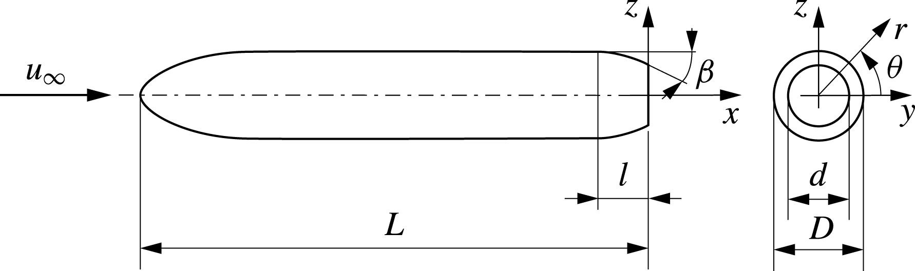
The boat-tailed bodies considered in the present investigation were obtained by modifying the axisymmetric body already analysed experimentally and numerically in Mariotti & Buresti (Reference Mariotti and Buresti2013) and in Mariotti, Buresti & Salvetti (Reference Mariotti, Buresti and Salvetti2015a
). It has a
 $3:1$
semi-elliptical forebody, a cylindrical main body and a sharp-edged flat base perpendicular to the axis. The ratio between the overall length,
 $L$
, and the main body diameter,
 $D$
, is
 $L/D=5.714$
. In the present case the last portion of the body is replaced with circular-arc boat tails of length
 $l$
, whose shapes are perfectly defined – and thus reproducible – once the diameter and length ratios,
 $d/D$
and
 $l/D$
, are given (see figure 1, where the reference axes, with origin at the centre of the base, are also shown).
Basic geometry of the analysed body.

The choice of the parameters defining the boat-tail geometry was based on the results of the seminal paper by Mair (Reference Mair1969), who found that the best results as regards the reduction of the base drag of axisymmetric bodies may be obtained by increasing the boat-tail angle
 $\unicode[STIX]{x1D6FD}$
– and thus by decreasing the diameter ratio
 $d/D$
for fixed boat-tail length
 $l/D$
– but only as long as the boundary layer remains attached over the boat-tail lateral surface. This condition was found to correspond to
 $\unicode[STIX]{x1D6FD}$
in the range
 $22\,^{\circ }{-}26\,^{\circ }$
for boat tails with a lateral profile approaching a circular arc and
 $l/D$
between
 $0.5$
and
 $0.65$
. The experiments in Mair (Reference Mair1969) were carried out at a Reynolds number
 $Re=u_{\infty }D/\unicode[STIX]{x1D708}=4.6\times 10^{5}$
and with a turbulent boundary layer having a thickness just before the boat tail of the order of
 $\unicode[STIX]{x1D6FF}/D=0.066$
. In the present investigation, considering also the limits of practical applications, it was decided to keep the length of all the analysed boat tails fixed at the value
 $l/D=0.5$
. The Reynolds number for both experiments and simulations was
 $Re=9.6\times 10^{4}$
and the characteristics of the boundary layer before the boat tail (at
 $x/D=-0.7$
), as derived from the data obtained during the experiments described in Mariotti & Buresti (Reference Mariotti and Buresti2013) and the VMS-LES simulations of Mariotti et al. (Reference Mariotti, Buresti and Salvetti2015a
), are given in table 1. In the table, the values of the boundary layer thickness,
 $\unicode[STIX]{x1D6FF}$
, displacement thickness,
 $\unicode[STIX]{x1D6FF}^{\ast }$
, and momentum thickness,
 $\unicode[STIX]{x1D703}$
, are reported. The differences between experiments and simulations are due to the level of turbulence present in the wind tunnel free stream, which is absent in the numerical simulations. In particular, the values of the shape factor
 $H=\unicode[STIX]{x1D6FF}^{\ast }/\unicode[STIX]{x1D703}$
show that the boundary layer is fully developed turbulent in the experiments and still transitional in the simulations.
Boundary layer characteristics upstream of the boat tail (
 $x/D=-0.7$
).

In the present work, the aim was to test the performance of the contoured grooves in delaying separation for a range of conditions, namely with boundary layers separating at different distances from the base sharp contour. A diameter ratio
 $d/D=0.791$
(corresponding to
 $(d/D)^{2}=0.625$
) was then chosen to be analysed both experimentally and numerically. For this configuration, the boat-tail angle was
 $\unicode[STIX]{x1D6FD}\approx 23.7\,^{\circ }$
. By comparison with the conditions of the experiments by Mair (Reference Mair1969), which were not far from those of the present wind tunnel tests, it could be predicted that in the experiments separation would occur almost at the end of the lateral surface. This experimental configuration was then expected to be the one with the most downstream separation position. Conversely, considering the different boundary layer conditions, a significantly more upstream separation should occur in the numerical simulations for the same boat tail. In order to assure that different separation conditions would be analysed in both the numerical and experimental campaigns, numerical simulations were also performed for boat-tailed bodies with
 $d/D=0.866$
(corresponding to
 $(d/D)^{2}=0.75$
and
 $\unicode[STIX]{x1D6FD}\approx 15.3\,^{\circ }$
) and wind tunnel tests were also carried out for models with
 $d/D=0.632$
(corresponding to
 $(d/D)^{2}=0.40$
and
 $\unicode[STIX]{x1D6FD}\approx 40.4\,^{\circ }$
). Compared to the
 $d/D=0.791$
configuration, the first one was expected to delay separation in the simulations thanks to the smaller boat-tail angle; conversely, due to the increased flow deviation, an anticipated separation could be expected in the experiments with the second boat tail. This guess was a posteriori confirmed by the experimental and numerical results described in § 3.
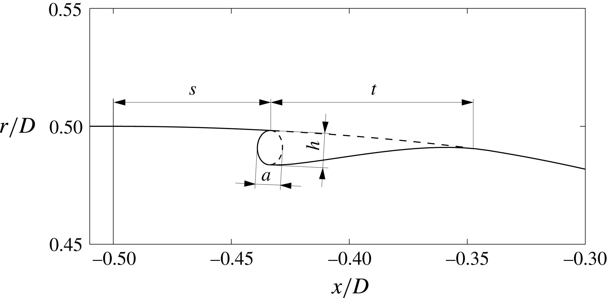
One axisymmetric contoured groove was then added to the lateral surface of each of the analysed boat tails. The geometry of a typical groove – shown in figure 2 – is analogous to the one of the cavities already introduced in Mariotti et al. (Reference Mariotti, Grozescu, Buresti and Salvetti2013). It starts with a sharp edge, has an upstream part with a semi-elliptical shape and ends with a spline tangential to the boat-tail lateral surface. The initial sharp edge is introduced to fix the start of a local recirculation region embedded in the lower part of the boundary layer. To avoid the appearance of phenomena of cavity oscillations and to assure the steadiness of the flow recirculation inside the cavity, the groove depth is chosen to be significantly smaller than the incoming boundary layer thickness. The absence of a sharp downstream edge and the gentle slope of the rear face produced by the spline also contribute to the production of a steady and stable flow. The steadiness of the recirculation region inside the cavity was indeed checked a posteriori (see § 3.3).
Considering that the length of the ellipse axis parallel to the diffuser,
 $a$
, had been found in Mariotti et al. (Reference Mariotti, Grozescu, Buresti and Salvetti2013) to have a small influence on the results, it was decided to connect its value to the depth of the groove by setting
 $a/h=2/3$
. The parameters defining the geometry of a groove are then its distance from the start of the boat tail,
 $s$
, its total length,
 $t$
, and its depth
 $h$
. In order to choose sensible values for these parameters, for each configuration subsequently analysed through the wind tunnel tests and the VMS-LES a preliminary numerical optimization procedure was carried out using a RANS code with a shear stress transport (SST)
 $k{-}\unicode[STIX]{x1D714}$
turbulence model. In these RANS simulations only the flow past the last portion of the body was evaluated and the objective function to be minimized was the boat-tail pressure drag. In order to reproduce the conditions of the experimental tests and VMS-LES simulations, the different velocity profiles corresponding to the boundary layer parameters reported in table 1 were used as inlet flow conditions. Furthermore, to assure the steadiness of the flow recirculating inside the grooves,
 $h$
was constrained to be smaller than
 $1/3$
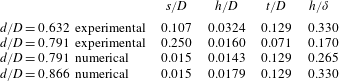
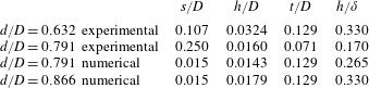
of the thickness of the boundary layer present just upstream of the boat tail. The resulting values of the groove parameters, which were subsequently used in the various cases, are shown in table 2. The different values of the parameters for the various cases are connected with the position of the boundary layer separation and the pressure distribution that characterize each boat tail and method of analysis. In particular, the parameter
 $s$
is smaller when the separation in the boat tail without groove occurs more upstream. In practice, in most cases the location of the groove was found to correspond to the region where the minimum pressure occurs on the lateral side of the plain boat tail (see also § 3.2).
Sketch of the groove geometry and main parameters.

Parameters of the grooves used in the experiments and simulations.
It must be emphasized that this preliminary activity was carried out only to devise CTG shapes that could reasonably be thought of as being effective in the subsequent experimental and numerical tests. However, due to the limited reliability of the RANS simulations in reproducing the detailed features of the base and wake flow of the analysed bodies, there is no claim that the parameters of table 2 correspond to actually optimized grooves. Indeed, a reliable optimization, which is obviously strongly configuration dependent, would require a higher-level numerical approach and huge computational costs. On the other hand, the objective of the present work was just to demonstrate the effectiveness of the use of CTGs to delay separation in different conditions – with consequent effects on drag according to the original body geometry – and not of providing an optimization of their shape. Nonetheless, as will be described in § 4, some supplementary VMS-LES simulations were carried out to obtain a first characterization of the robustness of the performance of CTGs to the variation of the parameters defining their shape.
2.2 Numerical methodology
The variational multiscale large-eddy simulations were carried out by using AERO, an in-house developed compressible flow solver. The code had already been successfully used for the simulation of bluff-body flows (see, e.g. Camarri et al.
Reference Camarri, Salvetti, Koobus and Dervieux2004; Ouvrard et al.
Reference Ouvrard, Koobus, Dervieux and Salvetti2010; Wornom et al.
Reference Wornom, Ouvrard, Salvetti, Koobus and Dervieux2011). The numerical discretization is based on a linearized implicit time advancing and on a mixed finite-volume/finite-element method, applicable to unstructured grids. The accuracy of the numerical method is second order both in space and in time and the Smagorinsky subgrid scale model is used to close the VMS-LES equations. The computational domain is cylindrical, with a diameter of 15
 $D$
and a length of 50
 $D$
(30
 $D$
being the distance of the outlet from the body base). This corresponds to a blockage factor of less than
 $0.5\,\%$
. The domain size was chosen on the basis of the settings of previous LES simulations of bluff-body flows, carried out with the same code and the same boundary conditions (see, e.g. Ouvrard et al.
Reference Ouvrard, Koobus, Dervieux and Salvetti2010), and of the sizes typically used in the literature for the numerical simulation of similar problems (see e.g. Bohorquez & Parras Reference Bohorquez and Parras2011 and the references therein).
As already mentioned, the simulations concern the isolated body of figure 1 with the boat tails
 $d/D=0.791$
and
 $d/D=0.866$
, with and without the grooves of table 2, at a Reynolds number
 $Re=u_{\infty }D/\unicode[STIX]{x1D708}=9.6\times 10^{4}$
and laminar free-stream conditions. No-slip is imposed over the body surface and characteristic-based boundary conditions (see e.g. Camarri et al.
Reference Camarri, Salvetti, Koobus and Dervieux2004) are used at the inflow, outflow and lateral boundaries of the computational domain. At the inflow, a uniform and time-constant velocity is assumed and the free-stream Mach number is set equal to
 $0.1$
, so that compressibility effects are negligible.
An unstructured grid having approximately
 $2.4\times 10^{6}$
nodes is used. The grid resolution around the body and in the near wake was selected on the basis of the previous LES simulations of the body without the boat tail, documented in Mariotti et al. (Reference Mariotti, Buresti and Salvetti2015a
), for which a grid sensitivity analysis was carried out. The grid is particularly refined near the body surface, where the wall
 $y^{+}$
is lower than 1, and in the near wake. The grooves considered in the present work are discretized by approximately 260 000 nodes. Finally, the adopted dimensionless time step is
 $\unicode[STIX]{x0394}T=\unicode[STIX]{x0394}t(u_{\infty }/D)\approx 4.5\times 10^{-3}$
. This time step is two orders of magnitude below the period of the dominating fluctuations present in the wake. Moreover, by defining the Courant–Friedrichs–Lewy (CFL) number in each cell as
 $\text{CFL}=\unicode[STIX]{x0394}t(u/\unicode[STIX]{x0394}x)$
, the adopted time step corresponds to a variable CFL, with a maximum value at each time step approximately equal to
 $2$
. This maximum CFL value is well below the stability limits of the adopted implicit time advancing scheme. All the flow statistics showed in the following were computed by neglecting an initial numerical transient and then by using a time interval of
 $65T$
 $(T=tu_{\infty }/D)$
. This interval corresponds to at least 15 hairpin shedding cycles in the wake (see § 3.4). Unless otherwise specified, the statistics are computed by also averaging in the homogeneous azimuthal direction. As in Mariotti et al. (Reference Mariotti, Buresti and Salvetti2015a
), an analysis of the convergence of the statistics of different quantities, such as the mean values of the boundary layer characteristic thicknesses, of the body base pressure coefficient or of the mean recirculation length, was carried out. As an example of convergence, by comparing the mean values of all these quantities computed over the above-mentioned time interval and over another one approximately
 $25\,\%$
shorter for the case
 $d/D=0.791$
, it was found that they differed by less than
 $1\,\%$
.
2.3 Experimental set-up
The tests were carried out in a closed-return, subsonic wind tunnel with a circular open test section 1.1 m in diameter and 1.42 m in length, with a free-stream turbulence level of
 $0.9\,\%$
; the Reynolds number was the same of the numerical simulations. The basic body used for the tests was the aluminium-alloy model already employed in Mariotti & Buresti (Reference Mariotti and Buresti2013), with diameter and overall length
 $D=70$
mm and
 $L=400$
mm. The final
 $1.5D$
long portion of the model, which was removable, was substituted with four acrylonitrile butadiene styrene (ABS) polymer elements, produced with a 3D printer, comprising the
 $0.5D$
long boat tails with
 $d/D=0.791$
and
 $d/D=0.632$
, both plain and with the grooves of table 2. The surface of the boat tails was polished with emery cloth after the printing process in order to obtain effectively smooth conditions with the correct dimensions.
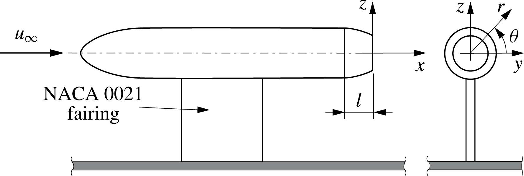
The models were supported above a flat plate by means of a faired strut (see figure 3). As already discussed in Mariotti & Buresti (Reference Mariotti and Buresti2013), this type of support was preferred to a rear sting support, which would directly interfere with the near-wake flow development. The drawback is that the flow is not symmetrical in the vertical plane, while it remains symmetrical in the horizontal plane. However, this did not impede to obtain a reliable comparison between the cases with and without grooves.
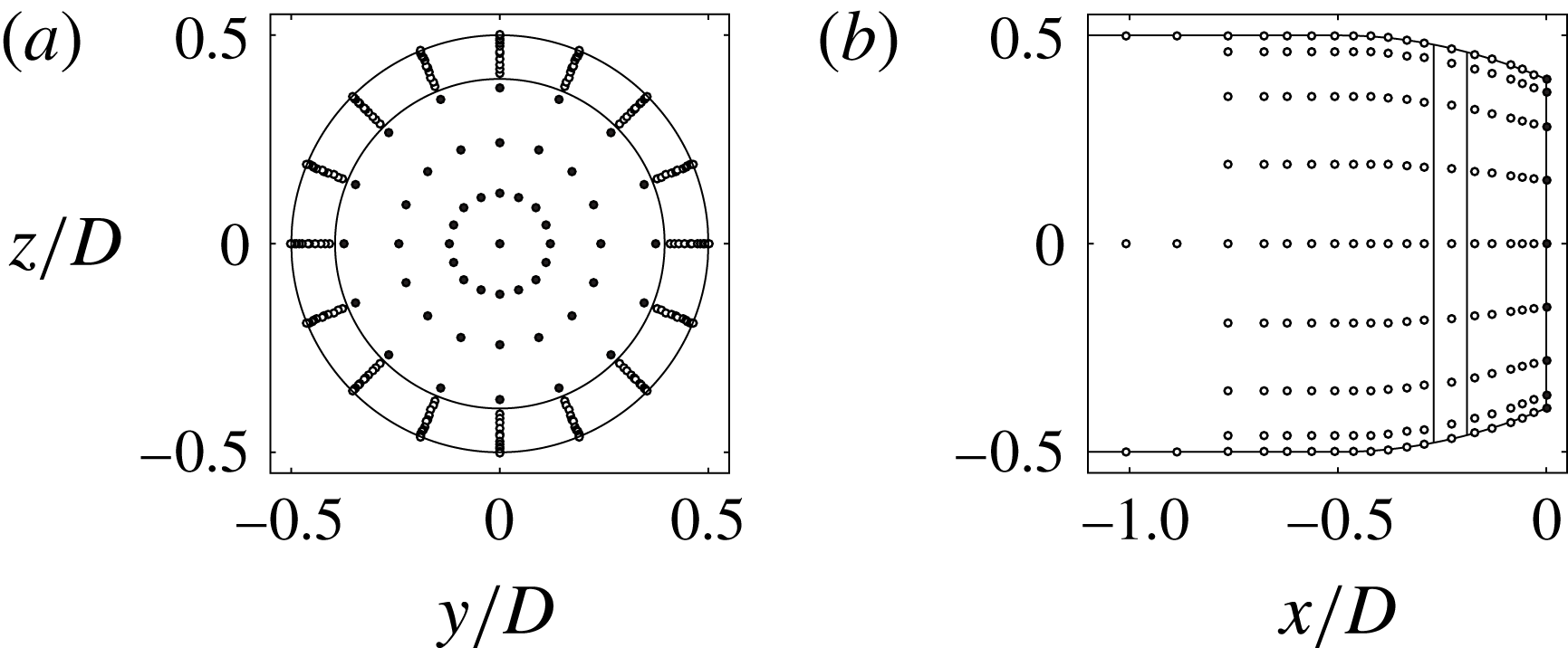
Each boat tail had 72 pressure taps over the lateral surface, distributed along four generatrix lines, and 49 taps over the base, along eight diametral lines. The pressures were measured using two Pressure Systems ESP-16HD miniature electronic pressure scanners, directly positioned inside the model with the relevant output cables passing through the support fairing. Through suitable rotations, the total number of measurement points was 288 over the lateral surface and 97 over the base, as shown in figure 4 for the boat tail with
 $d/D\approx 0.632$
. The number of pressure measurement points was sufficient to permit to obtain, by integration, reliable values of the contributions of the lateral surface and of the base to the pressure drag. Symmetrical pressure taps were also present on two perpendicular planes over the forebody surface in order to accurately align the model with the free stream.
The velocity measurements to obtain the boundary layer profiles and the wake field were carried out using an IFA AN 1003 A.A. Lab System hot-wire anemometry module. Single-wire Dantec 55P11 probes could be moved in the
 $x$
,
 $y$
and
 $z$
directions with an accuracy of 0.1 mm by means of a computer-controlled traversing system. After suitable preliminary tests, a sampling frequency of 2 kHz and a time length of approximately 65 s were chosen for the pressure and hot-wire signal acquisitions; this permitted to obtain stationary values of the moments up to the third order for all the fluctuating quantities.
Sketch of the experimental set-up.

Pressure measurement points (
 $d/D=0.632$
): (a) rear view, (b) lateral view.

3 Results
3.1 Drag reduction
The distribution of the pressure coefficient over the boat-tail surface was obtained from the local measured or calculated pressure
 $p$
and the free-stream pressure
 $p_{\infty }$
from the formula
 $$\begin{eqnarray}C_{p}=\frac{p-p_{\infty }}{1/2\unicode[STIX]{x1D70C}u_{\infty }^{2}},\end{eqnarray}$$
where
 $\unicode[STIX]{x1D70C}$
is the fluid density.
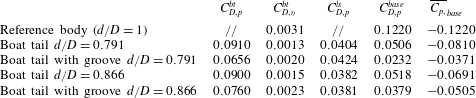
Numerical pressure and viscous contributions to mean drag coefficient (positive values correspond to drag) and base pressure coefficient,
 $\overline{C_{p,}}_{base}$
averaged in time and over the base (negative values correspond to suctions). Results for the reference body from Mariotti et al. (Reference Mariotti, Buresti and Salvetti2015a
).
The total mean pressure drag coefficient may be computed by integration over the body of the time-averaged pressure coefficients multiplied by the axial component of the outer normal unit vector divided by the reference body cross-section area
 $S=\unicode[STIX]{x03C0}D^{2}/4$
. The contributions to the total mean pressure drag coefficient associated with the various surfaces were then evaluated by the same integration over the relevant surface portions and subsequent division by
 $S$
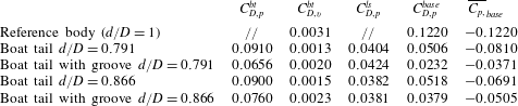
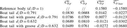
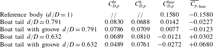
. In the experimental cases, the number of pressure taps was sufficiently high to allow a reliable continuous distribution over the various boat-tail surfaces to be obtained through a preliminary interpolation before carrying out the integrations. The boat-tail mean drag coefficients obtained in the simulations and in the experiments are reported in tables 3 and 4, respectively. Besides the total boat-tail mean pressure drag coefficient,
 $C_{D,p}^{bt}$
, the tables contain also the relevant contributions of the lateral surface,
 $C_{D,p}^{ls}$
, and of the base,
 $C_{D,p}^{base}$
. The mean base pressure coefficient,
 $\overline{C_{p,}}_{base}$
, averaged in time and over the base, is also given in the last column. Furthermore, as the numerical simulations provided also the mean viscous stresses
 $\unicode[STIX]{x1D70F}_{w}$
acting over the boat-tail surface, their contribution to the boat-tail mean drag coefficient,
 $C_{D,v}^{bt}$
, obtained by integration over the axial projection of the lateral surface and division by the reference area
 $S$
and the free-stream dynamic pressure, is also shown in table 3. Finally, in order to permit to appreciate the significant drag reduction performance of boat tailing, in the first row of both tables the mean pressure drag coefficients and the mean base pressure coefficients of the reference case without boat tail, obtained in previous works, are also reported; the corresponding value of the mean viscous drag contribution in table 3 refers to the last
 $0.5D$
long portion of the lateral surface.
As can be seen, in all cases the introduction of the groove leads to a reduction of the total mean drag coefficient of the boat tail, with per cent values that depend on the particular case and range from a minimum slightly above
 $5\,\%$
to a maximum of
 $29\,\%$
. The differences between the various cases depend on the conditions of the flow around the boat tail before the introduction of the groove and on the balance between the contributions of the lateral surface and of the base to the total boat-tail drag, as will be shown in more detail in the following part of this section. Furthermore, table 3 shows that in all cases the contribution to mean drag of the viscous stresses is at least one order of magnitude lower than the one of the pressures.
Experimental pressure contributions to the mean drag coefficient (positive values correspond to drag) and base pressure coefficient,
 $\overline{C_{p,}}_{base}$
averaged in time and over the base (negative values correspond to suctions). Results for the reference body from Mariotti & Buresti (Reference Mariotti and Buresti2013).
3.2 Mean pressure and velocity fields
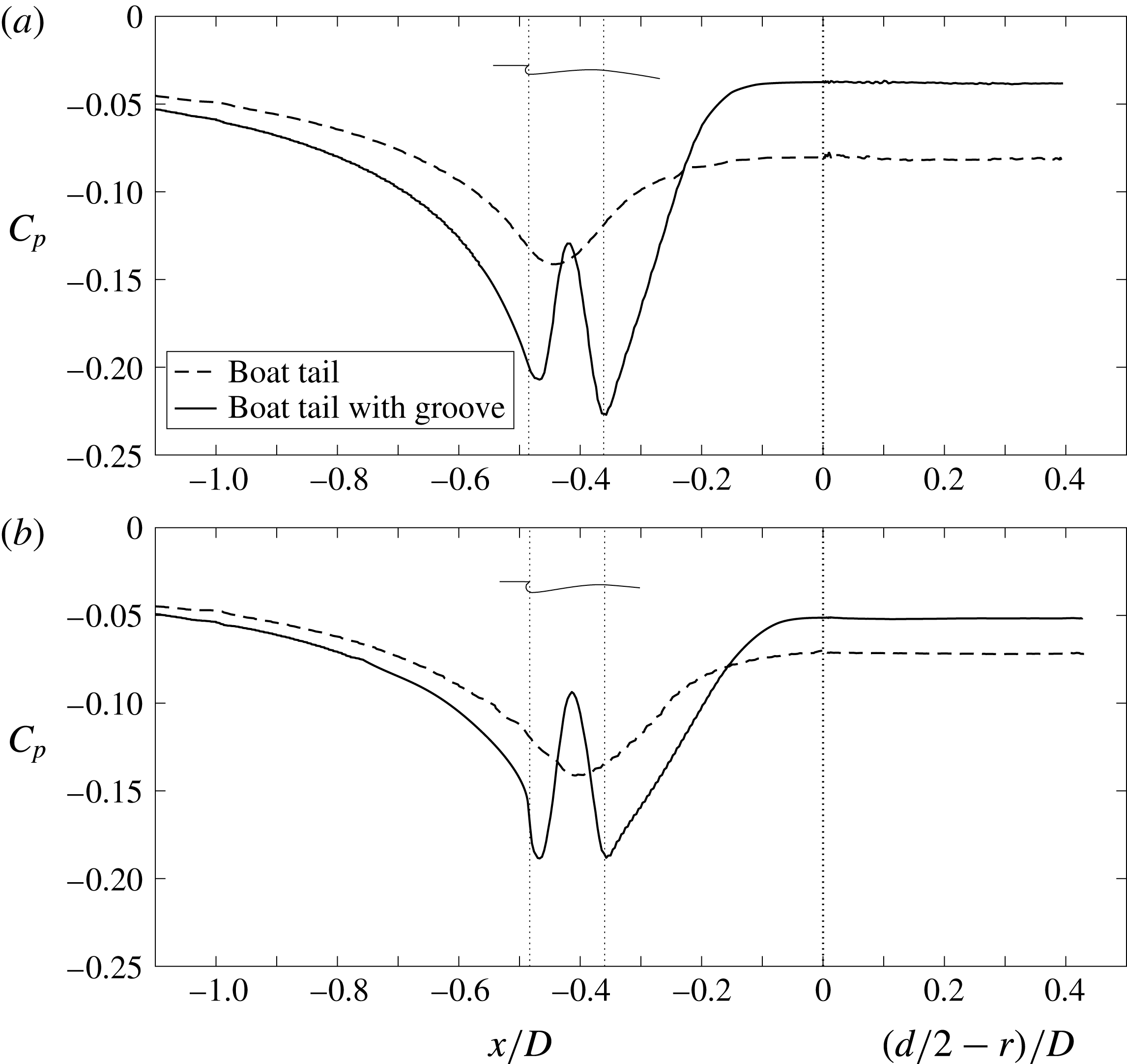
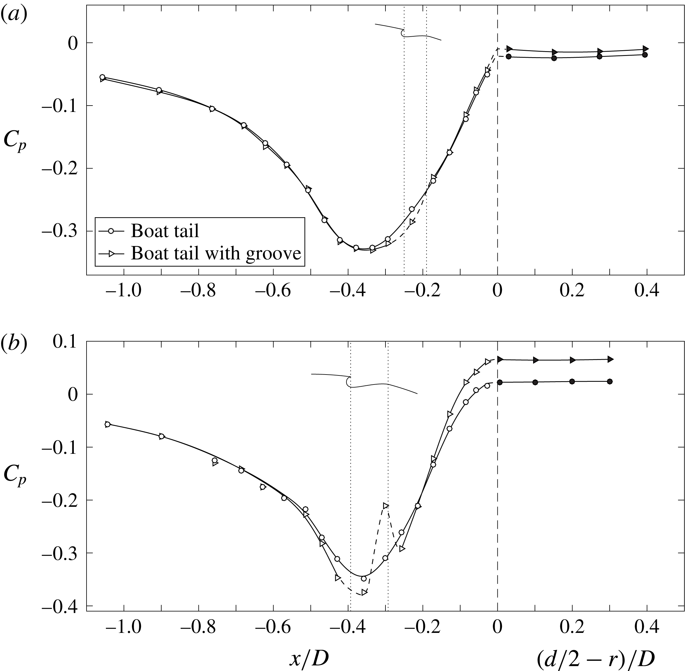
In order to better understand the behaviour of the different contributions to the mean pressure drag, we now analyse the mean pressure and velocity fields over the body and in the near wake, starting with the results of the VMS-LES simulations. The mean pressure distributions over the lateral boat-tail surface and over the base are shown in figure 5 for the various analysed cases. The left-hand part of these figures provides the values of the pressure coefficient along the last portion of the lateral surface of the body, in which the start of the boat tail is at
 $x/D=-0.5$
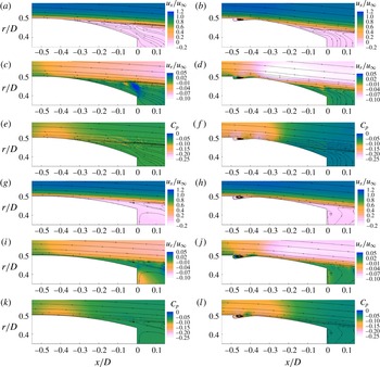
. The rightmost part of the figures shows the variation of the pressure along the radius of the base, starting from its border, in continuation to the values along the lateral surface. In each figure two vertical lines and a sketch indicate the position of the groove. Figure 6 provides a global description of the mean axial and radial velocity components and of the mean pressure field for the numerically analysed configurations; some streamlines are also superposed on the figures to help in the analysis of the differences between the various flow fields.
Let us first analyse the behaviour of the boat tails without the groove. As predicted, both configurations correspond to conditions with early flow separation, as it is evident from figure 6(a,c,e,g,i,k). Moreover, the pressure distributions over the lateral boat-tail surfaces and over the base provide different contributions to the drag according to the geometry and flow conditions. For instance, one can observe from table 3 that the two very similar total pressure drags of the plain boat tails with
 $d/D=0.791$
and
 $d/D=0.866$
correspond to rather different values of the base pressure coefficient. Indeed, the more downstream separation of the boat tail with
 $d/D=0.866$
leads to lower base suctions but its larger base area produces a slightly higher drag contribution than the one provided by the smaller base area of the boat tail with
 $d/D=0.791$
; however, the opposite occurs for the drag contributions of the lateral boat-tail surfaces.
Numerical pressure coefficient over the lateral surface and the base, averaged in time and in the azimuthal direction: (a)
 $d/D=0.791$
, (b)
 $d/D=0.866$
.

Numerical fields and velocity streamlines averaged in time and in the azimuthal direction. (a,b,g,h)
 $x$
-velocity, (c,d,i,j) radial velocity, (e,f,k,l) pressure coefficient. (a–f)
 $d/D=0.791$
, (g–l)
 $d/D=0.866$
.

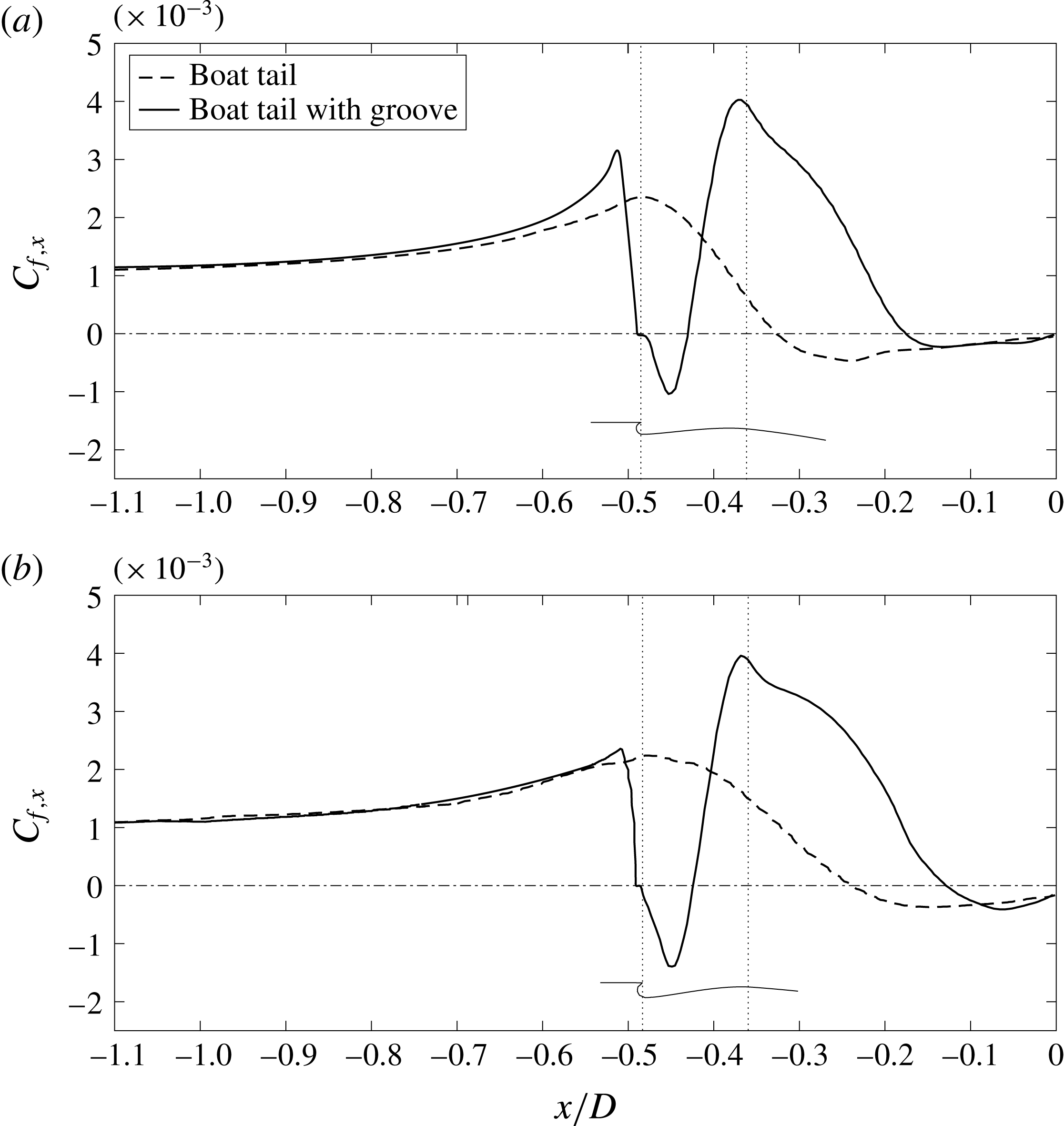
Numerical axial wall shear stress over the lateral surface averaged in time and in the azimuthal direction: (a)
 $d/D=0.791$
, (b)
 $d/D=0.866$
.

The modifications produced by the grooves are evident. In both cases a significant separation delay is produced by the introduction of the grooves, as can be seen in figure 6(b,d,f,h,j,l). The separation points may more quantitatively be derived by analysing the axial contribution of the mean friction coefficient
 $C_{f,x}=\unicode[STIX]{x1D70F}_{w}(\boldsymbol{t}\boldsymbol{\cdot }\boldsymbol{e}_{x})/(1/2\unicode[STIX]{x1D70C}u_{\infty }^{2})$
, where
 $\boldsymbol{t}$
and
 $\boldsymbol{e}_{x}$
are, respectively, the tangential and axial unit vectors. Figure 7 shows
 $C_{f,x}$
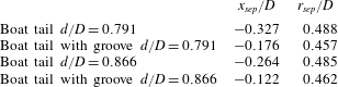
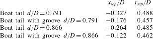
along the lateral surface of the boat tails; the position of the grooves is also indicated in the figure. The friction is obviously negative within the grooves, due to the flow recirculation, but the separation points may be assumed to coincide with the more downstream positions where the friction becomes negative, and their coordinates are reported in table 5. It can be inferred that the delay of separation is related to the enhanced pressure recovery in the last part of the body, leading to a larger base pressure, as can be observed in figure 5, and, more qualitatively, also from figure 6. However, let us now analyse more in detail the pressure distribution over the boat-tail surface and the base shown in figure 5. The presence of the grooves causes an earlier and enhanced decrease of the pressure before and at the beginning of the boat tail. However, a rapid increase in pressure occurs around the reattachment region after the recirculation inside the groove, followed by another decrease due to the subsequent acceleration of the flow. Finally, as already pointed out, the pressure recovery corresponding to the flow deceleration is much steeper when the grooves are present, leading to a significantly higher pressure at separation, which remains constant over the whole base.
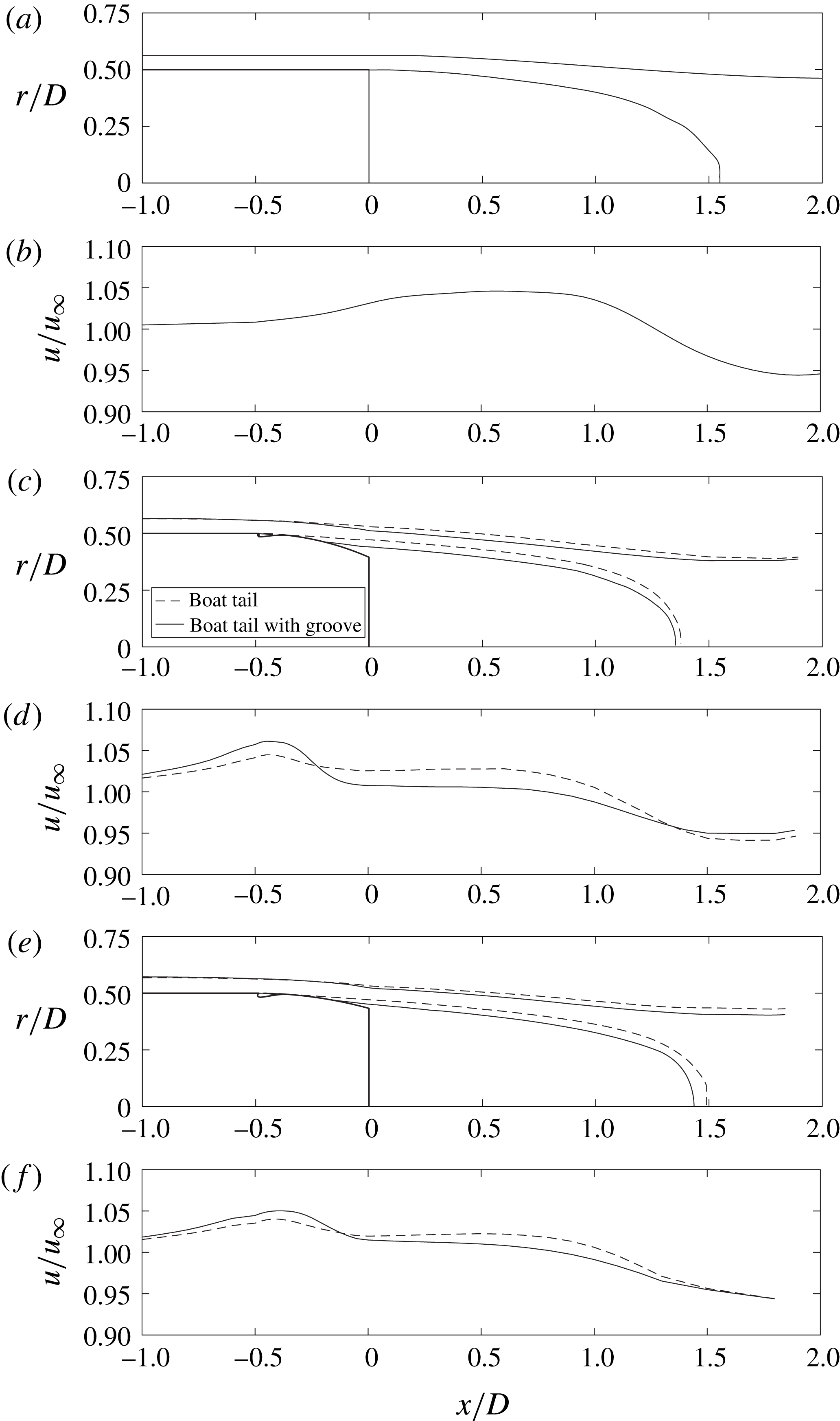
Boundary layer and wake borders and mean recirculation region, averaged in time and azimuthal direction. (a) Body without boat tail, (c)
 $d/D=0.791$
, (e)
 $d/D=0.866$
. Mean velocity distribution along the edges of the boundary layer and of the near wake: (b) body without boat tail, (d)
 $d/D=0.791$
, (f)
 $d/D=0.866$
.

Numerical separation points.
Experimental pressure coefficients in the horizontal plane: (a)
 $d/D=0.791$
, (b)
 $d/D=0.632$
. White and black symbols correspond to measurements over the lateral surface and the base, respectively.

Experimental standard deviation of the pressure coefficient over the lateral surface and the base in the horizontal plane: (a)
 $d/D=0.791$
, (b)
 $d/D=0.632$
. White and black symbols correspond to measurements over the lateral surface and the base, respectively.

A better understanding of this behaviour can be derived from the analysis of figure 8. In particular, 8(a), 8(c) and 8(e) show, respectively for the basic body without boat tail and for the two analysed boat-tailed bodies with and without grooves, the mean flow streamlines bounding the recirculation region, together with the boundary layer and near-wake edges evaluated as the positions corresponding to
 $99\,\%$
of the integral of the vorticity in the cross-flow direction. Furthermore, figure 8(b,d,f) shows, for the same cases, the magnitude of the mean velocity along the boundary layer and near-wake edges. The importance of the curvature of the outer contour of the boundary layer and of the near wake may be clearly deduced from these figures. Indeed, the mean recirculation region and the outer wake edge of the basic blunt-based body have an initial convex curvature, which produces an increase of the velocity starting before the end of the body and continuing up to a position of maximum velocity in the near wake. Subsequently, the velocity starts to decrease, following the change of the curvature of the outer streamlines. The important point is that the value of the pressure over the base practically coincides with the one just outside the boundary layer separating at the base contour, which, in turn, is directly connected with the value of the velocity in the same position. The effective coincidence between mean pressure outside the separating boundary layer and over the base was also found for the boat-tailed bodies, and this immediately connects the base pressure with the velocity present along the wake edge at the coordinate corresponding to the body base (
 $x/D=0$
). The effect of boat tailing is thus seen to be due to the fact that the maximum of the velocity and its subsequent decrease due to the changes in streamline curvature occur considerably in advance compared to the basic body. Therefore, it is seen that an earlier change to a concave curvature of the outer streamlines is the mechanism through which boat tailing causes an increase in base pressure. The effect of the grooves is to enhance this mechanism by further delaying the boundary layer separation and thus reducing the outer velocity at the edge of the base, as may be seen in figure 8(d,f). From table 5, it can be noticed that the
 $d/D=0.791$
boat tail with the groove has a somewhat earlier boundary layer separation than the corresponding one with
 $d/D=0.866$
; nonetheless, the higher pressure recovery in the last part of the boat tail derives from a larger streamline curvature caused by the smaller wake width connected with the radial position of the separation point (see figure 8). Consequently, the introduction of the groove for the
 $d/D=0.791$
case leads to a significantly higher pressure recovery than occurs for the grooved boat tail with
 $d/D=0.866$
; this is sufficient to cause a considerable decrease of the base suctions which produces, in spite of the smaller base area, a larger reduction of the base drag and, consequently, a definitely smaller total pressure drag.
Finally, it is interesting to observe that Mariotti et al. (Reference Mariotti, Buresti and Salvetti2015a ) found that, for the basic body without boat tail, the base pressure is an increasing function of the length of the recirculation region (see also Barros et al. Reference Barros, Borée, Noack, Spohn and Ruiz2016 for a three-dimensional non-axisymmetric blunt body). This is a consequence of the direct connection between velocity outside the separating boundary layer and convex curvature of the initial near-wake boundary, which increases when the recirculation length decreases. However, this direct connection is no longer evident in the case of boat-tailed bodies, for which the streamlines outside the separating shear layers are generally characterized by a concave curvature; consequently, as may also be deduced from figure 8, the length of the recirculation region is now a non-trivial function of the radial position and surface inclination of the boundary layer separation position and of the curvature of the outer streamlines in that location.
As for the experimental data, the pressure distributions obtained for the different cases are shown in figure 9. The first point to be noted is that the case with
 $d/D=0.791$
is the one for which the groove provides the minimum variation of the pressure distribution, and thus of the drag reduction. This is actually not surprising, because, as already pointed out in § 2, considering the turbulence level of the wind tunnel this configuration was expected to correspond to an almost completely attached flow over the boat-tail lateral surface of the reference model. Consequently, the introduction of the groove may only produce the slight downstream movement of the separation point necessary for it to reach the base edge and its effect on the pressure distribution and drag is limited. Conversely, for the reference case with
 $d/D=0.632$
the diameter ratio is sufficiently small to induce a boundary layer separation over the lateral surface well before the base contour. Therefore, the effect of the groove is much more significant, allowing a stronger downstream recompression to be obtained (see figure 9
b). It should be noted that for this smaller diameter ratio the recompression along the lateral surface is always sufficiently strong to lead to positive values of the pressure coefficient, which act over the last portion of the lateral surface and over the base. Therefore, although this configuration corresponds to an anticipated flow separation, even for the boat tail without groove the resulting drag is definitely lower than for the
 $d/D=0.791$
configuration.
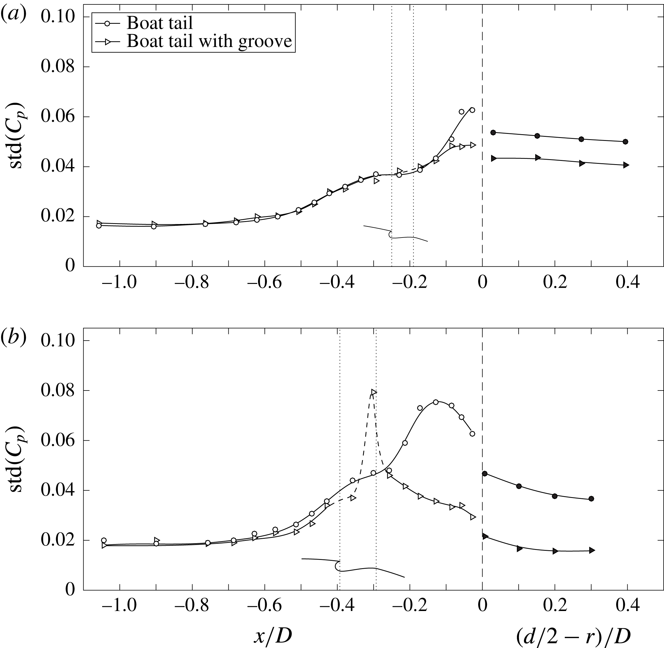
No measurement allowing a direct detection of the separation point was available in the experiments; however, the different positions of the boundary layer separation for the experimental cases may be inferred from the values of the pressure standard deviation along the lateral surface, which are shown in figure 10. Indeed, it is reasonable to suppose that the region of separation be connected with an increase of the pressure fluctuations. As can be seen in figure 10(a), for the plain boat tail with
 $d/D=0.791$
the increase occurs only at the very end of the lateral surface, thus confirming the fact that this configuration corresponds to a nearly completely attached flow. Nonetheless, the reduction of the pressure fluctuations in that same region and over the base caused by the introduction of the groove suggests its full effectiveness in producing a totally attached flow. A definitely different situation corresponds to the
 $d/D=0.632$
configuration (see figure 10
b). Indeed, for this diameter ratio the plain boat tail shows a significant increase of the fluctuations over the rear part of the lateral surface, indicating a flow separation occurring before the base. The introduction of the groove has thus a notable effect and the data seem to indicate that separation is now practically avoided, as is also witnessed by the remarkable decrease of the pressure fluctuations over the last portion of the lateral surface and over the base. The local peak that occurs near
 $x/D=-0.3$
, which corresponds to the final part of the groove profile, will be discussed in § 3.3.
Boundary layer and wake flow features in the horizontal plane: the black and white symbols correspond to the peaks of the skewness and of the standard deviation, respectively: (a)
 $d/D=0.791$
, (c)
 $d/D=0.632$
. Mean velocity distribution along the edges of the boundary layer and of the near wake: (b)
 $d/D=0.791$
, (d)
 $d/D=0.632$
.

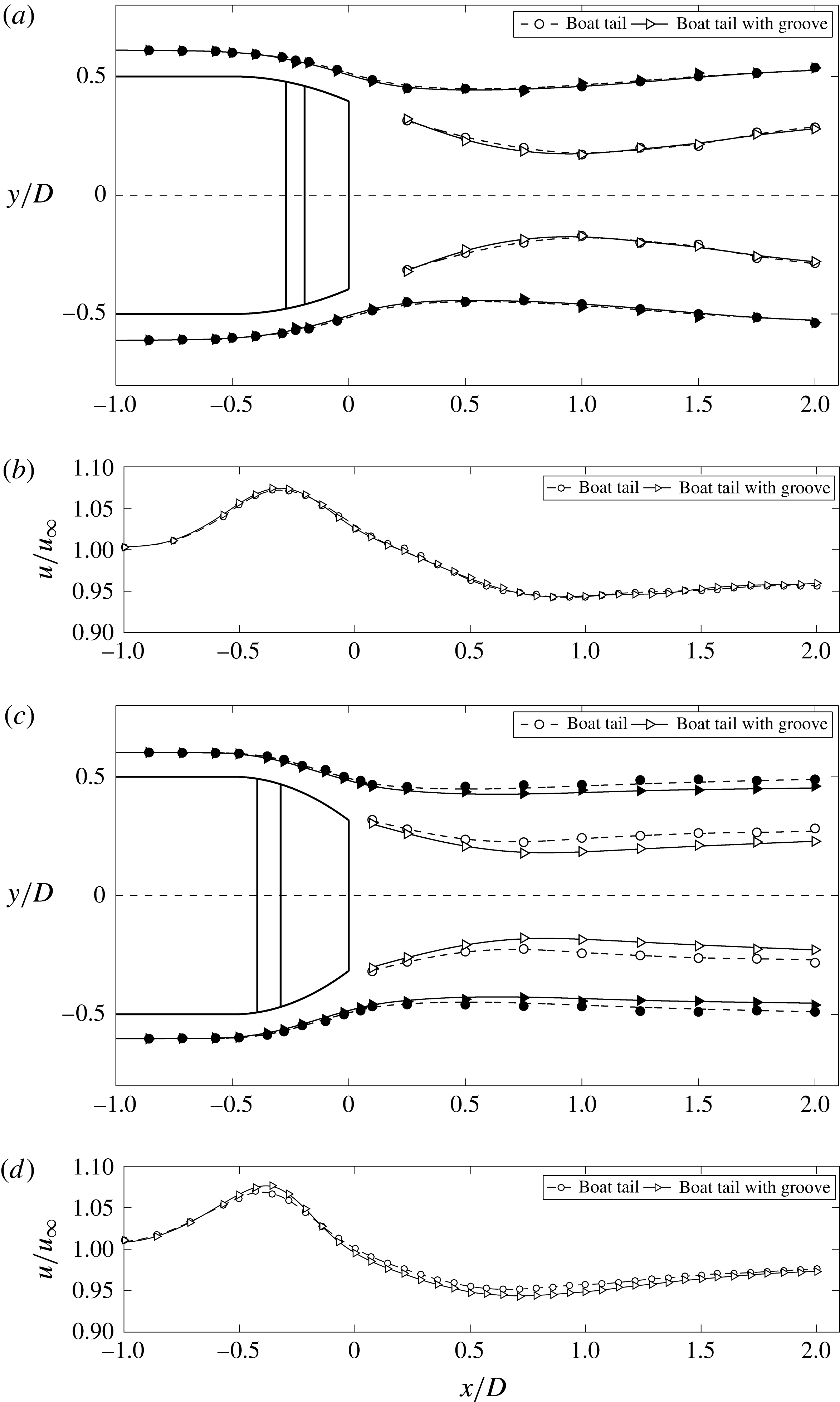
For the two diameter ratios analysed experimentally, the general effect of the grooves may also be derived from figure 11 showing the wake configurations. In this figure, the edges of the boundary layers and of the wakes are identified through the lines corresponding to the negative peaks of the skewness of the velocity fluctuations. For the reasons already explained in detail in Mariotti & Buresti (Reference Mariotti and Buresti2013), using the variation of the skewness when some level of turbulence is present in a flow provides accurate estimates of the boundary layer thicknesses and of the wake widths. As a further indication of the wake widths, in figure 11 the lines connecting the maxima of the velocity standard deviation are also reported. As can be appreciated, for
 $d/D=0.791$
the reduction of the width of the wake produced by the introduction of the groove is almost imperceptible. Conversely, the wake narrowing effect is perfectly evident for
 $d/D=0.632$
, thus confirming the much more significant separation-delay effect of the groove for this configuration. The magnitude of the velocity along the outer edge of the boundary layer and near wake are also shown in figure 11; as happened for the numerical simulations in figure 8, the variation of the curvature of the outer streamlines implies that the velocity is characterized by an initial acceleration and by a subsequent deceleration, which determines the value of the base pressure.
Numerical boundary layer
 $x$
-velocity profiles averaged in the azimuthal direction for
 $d/D=0.791$
. Mean value at (a)
 $x/D=-0.50$
, (b)
 $x/D=-0.46$
, (c)
 $x/D=-0.35$
; standard deviation at (d)
 $x/D=-0.50$
, (e)
 $x/D=-0.46$
, (f)
 $x/D=-0.35$
.

Experimental boundary layer
 $x$
-velocity profiles in the horizontal plane for
 $d/D=0.632$
. Mean value at (a)
 $x/D=-0.45$
, (b)
 $x/D=-0.37$
, (c)
 $x/D=-0.28$
; standard deviation at (d)
 $x/D=-0.45$
, (e)
 $x/D=-0.37$
, (f)
 $x/D=-0.28$
.

3.3 Mechanism of action of the groove
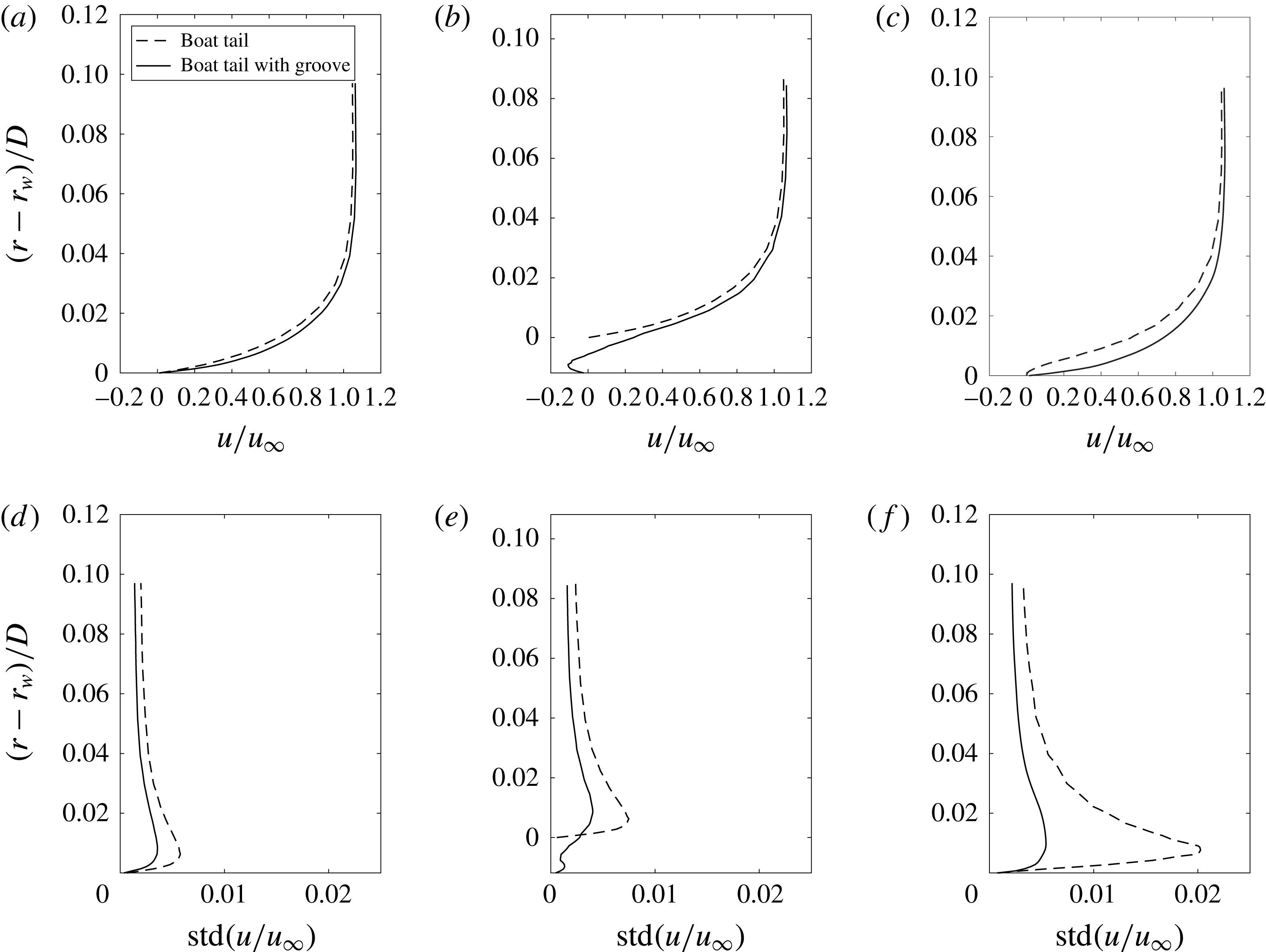
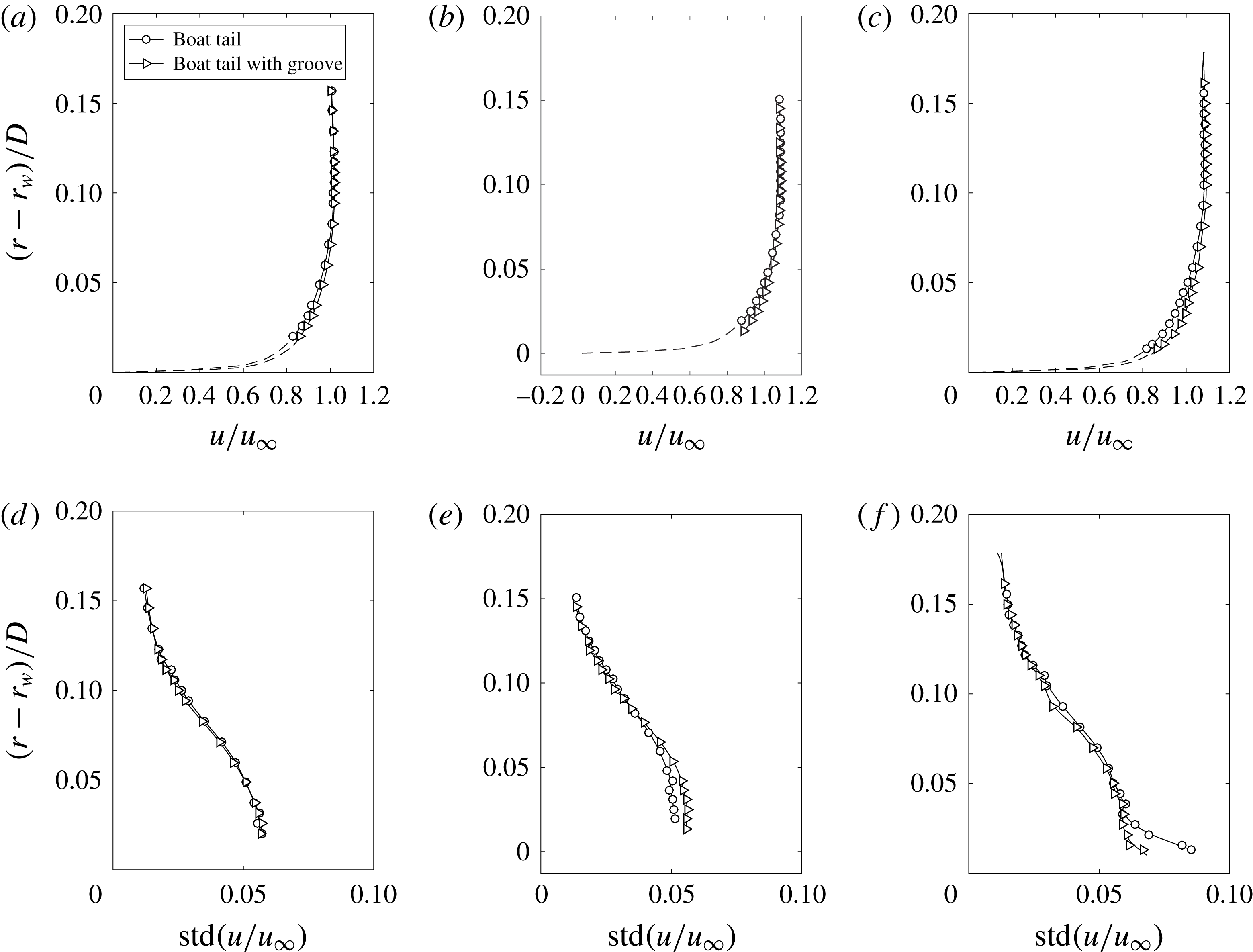
In § 3.2 it was shown that, in all cases, the introduction of the grooves delays the boundary layer separation over the body lateral surface. We now analyse possible explanations of the origin of this effect. To this end, we start by considering the velocity field of three representative boundary layers, namely those placed just upstream, in the mid and immediately downstream of the grooves. For these positions, the profiles of the mean value and of the standard deviation of the axial velocity are shown in figure 12 for the numerical configurations with
 $d/D=0.791$
and in figure 13 for the experimental cases with
 $d/D=0.632$
. In the figures the coordinate
 $r_{w}$
corresponds to the local radial position of the plain boat-tail surface. The correspondence between the axial coordinates referred to in the captions of the figures and the above cited characteristic positions may be verified from the sketches of the grooves included in figures 5(a) and 9(b). Due to practical measurement limitations, the experimental data reported in figure 13 do not extend down to the surface and thus an extrapolation is carried out below the available data nearest to the surface using the Reichardt wall law (Reichardt Reference Reichardt1951). The extrapolation is not introduced for the profile within the groove. Conversely, the numerically obtained profiles of figure 12 are obviously complete.
The first observation that is evident from figure 12(a,c) is the higher mean near-wall momentum of the velocity profiles of the boat tail with groove compared to that of the profiles corresponding to the same axial coordinates for the plain boat tail. The increase is limited upstream of the groove (figure 12
a) but becomes significant in the downstream position (figure 12
c). More interestingly, figure 12(b) permits us to appreciate that the recirculation inside the groove causes a significant slip velocity to be present over the groove at the radial coordinate corresponding to the surface of the boat tail without the groove (
 $r=r_{w}$
). Actually, the corresponding velocity is seen to be of the order of
 $0.2u_{\infty }$
. This effect immediately justifies the stronger resistance to separation of the boundary layer developing downstream of the groove. In spite of the lower number of measurement points, the same enhancement of the near-wall momentum is clearly visible also in figure 13 for the experimental configurations.
Comparison between the numerical boundary layer characteristic thicknesses before the groove (
 $x/D=-0.5$
) and after the groove (
 $x/D=-0.35$
) for
 $d/D=0.791$
.

Comparison between the experimental boundary layer characteristic thicknesses before the groove (
 $x/D=-0.45$
) and after the groove (
 $x/D=-0.28$
) in the horizontal plane for
 $d/D=0.632$
.

The effect of the introduction of the grooves on the boundary layer mean velocity profile is concisely described by the parameters reported in tables 6 and 7, respectively for the numerical and the experimental configurations. The characteristic thicknesses and the shape factors are shown for the positions immediately upstream and downstream of the grooves. As is apparent, the effect of the groove is to produce a decrease of the thickness of the boundary layer. Note that the displacement thickness and the shape factor are also reduced and this is consistent with an increase of the distance from the separation condition.
We now enquire whether the increase in near-wall momentum observed downstream of the recirculations may be connected with enhanced flow fluctuations induced by the grooves. As a first remark, the profiles of the standard deviation of the velocity obtained in the numerical simulations, reported in figure 12(d–f), show a decrease of the velocity fluctuations within the boundary layer when the groove is present for all the considered positions. Particularly remarkable is the decrease of the near-wall turbulence intensity after the groove, but a reduction of the fluctuations is present also at the upper edge of the boundary layer.
The experimental data of figure 13(d–f) are not as clear, perhaps due to the pre-existing free-stream turbulence level; nonetheless, a reduction of the near-wall fluctuations after the groove is apparent and no increase may ever be observed outside the boundary layers. As for the extremely limited increase in the velocity fluctuations that may be observed in figure 13(e) in the inner part of the boundary layer above the mid of the groove, it corresponds to a position where an increased mean velocity also occurs, as shown in figure 13(b). Consequently, the variation of the local relative fluctuation level is smaller than that of the absolute level. It must be pointed out that these data are in agreement with those of figure 10(b), which show a remarkable reduction of the pressure fluctuations after the groove compared to those present over the plain boat tail. The local peak of pressure fluctuations that occurs in that figure at
 $x/D=-0.31$
, which corresponds to the final part of the groove profile, is most probably due to the fact that the related pressure tap practically coincides with the location of the reattachment of the streamline bounding the small recirculation region produced by the groove. This may be deduced not only from the sketch embedded in the figure, but also from the increased mean pressure that is found in figure 9(b) for the same pressure tap. In effect, it is well documented that the position of the reattaching streamline is normally close to a region where a high value of the fluctuations occurs (see, e.g. Taylor, Gurka & Kopp Reference Taylor, Gurka and Kopp2014). However, this increased fluctuation is extremely localized and it is remarkable to observe that, conversely, a decreased pressure fluctuation is found for the immediately preceding pressure tap (at
 $x/D=-0.37$
), which is located well inside the groove, and thus, presumably, beneath the recirculation region (see figure 10
b).
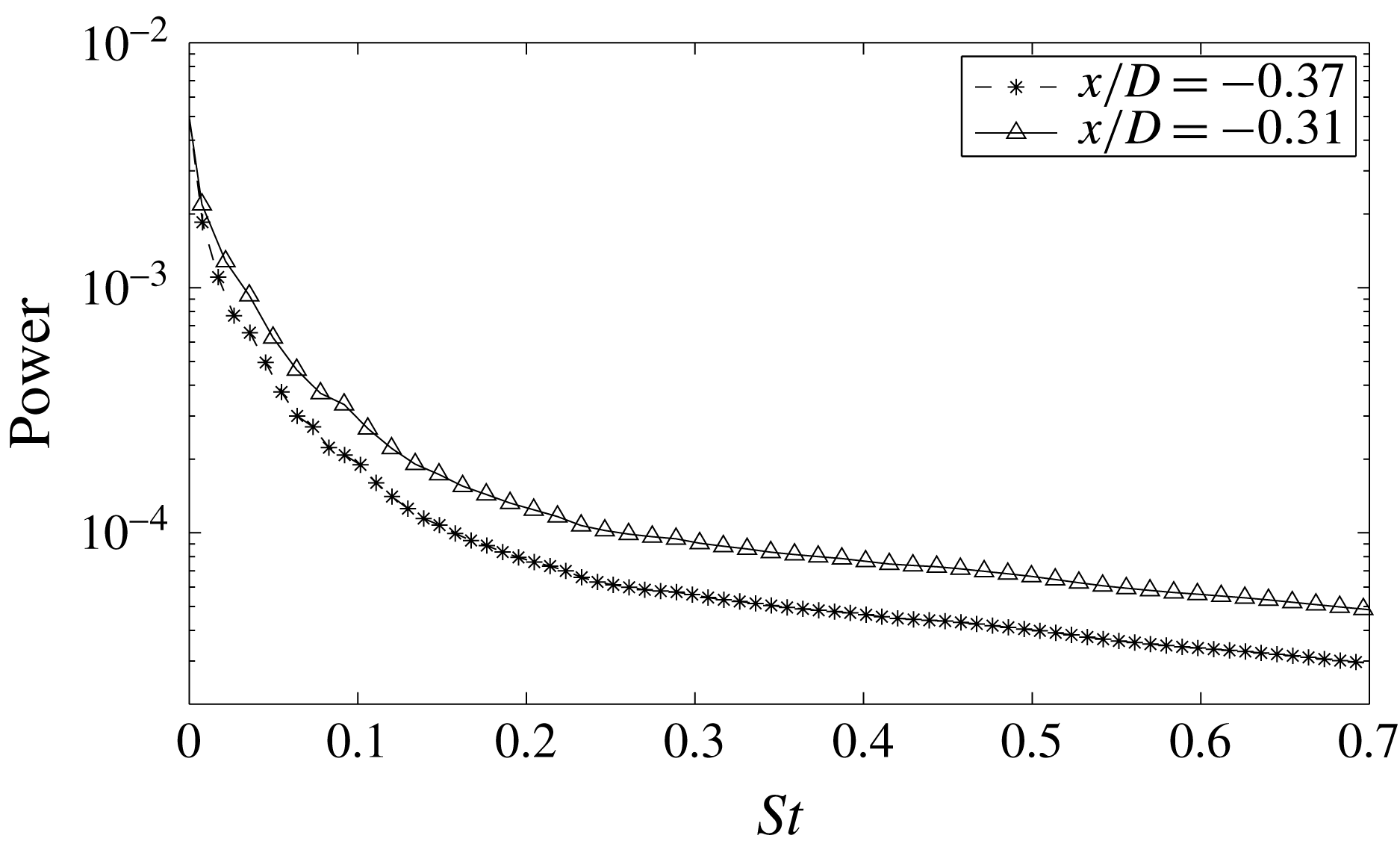
Finally, figure 14 shows the experimental spectra of the velocity fluctuations in the boundary layer over the two above mentioned positions, in terms of a Strouhal number
 $St=fD/u_{\infty }$
. The spectra are derived from the wavelet transform of the velocity signals, by integrating in time the wavelet maps obtained by employing the complex Morlet wavelet
 $\unicode[STIX]{x1D6F9}(t)=\text{e}^{\text{i}\unicode[STIX]{x1D714}_{0}t}\text{e}^{-t^{2}/2}$
and using a central frequency
 $\unicode[STIX]{x1D714}_{0}=6\unicode[STIX]{x03C0}$
in order to enhance the frequency resolution. This procedure permits us to obtain spectra that are smoother than the Fourier ones and well defined from the mathematical point of view. No peak is present in the spectra, indicating once again that no cavity resonance phenomena are present. Similar conclusions can be drawn from velocity signals recorded in other surrounding measurement locations and from the numerical simulations (not shown here for the sake of brevity). In summary, the available evidence strongly corroborates the inference that the small recirculation region present within the grooves is effectively steady.
Wavelet spectra of the velocity signal in the boundary layer (
 $(r-r_{w})/D=0.08$
) at
 $x/D=-0.31$
and
 $x/D=-0.37$
for the
 $d/D=0.632$
boat tail.

In order to get a deeper insight into the physical mechanisms through which the introduction of the grooves causes a delay of the boundary layer separation and a consequent mean drag reduction, it may also be interesting to evaluate the variation of dissipation
 $D_{T}$
occurring in the whole flow field. To this end, the Bobyleff–Forsyth formula is used (see, e.g. Serrin Reference Serrin and Flügge1959), in the alternative form introduced by Buresti (Reference Buresti2012):
 $$\begin{eqnarray}D_{T}=\int _{v}\unicode[STIX]{x1D719}\,\text{d}v=\unicode[STIX]{x1D707}\int _{v}\unicode[STIX]{x1D714}^{2}\,\text{d}v-2\unicode[STIX]{x1D707}\int _{\unicode[STIX]{x1D6F4}}\frac{\unicode[STIX]{x2202}(p/\unicode[STIX]{x1D70C})}{\unicode[STIX]{x2202}n}\,\text{d}\unicode[STIX]{x1D6F4}.\end{eqnarray}$$
In this formula, which is valid for an incompressible flow,
 $\unicode[STIX]{x1D719}$
is the dissipation function,
 $v$
a generic volume of fluid bounded by surface
 $\unicode[STIX]{x1D6F4}$
,
 $\unicode[STIX]{x1D714}^{2}$
is the enstrophy, i.e. the square modulus of the vorticity vector,
 $\unicode[STIX]{x1D707}$
is the viscosity of the fluid, and
 $\unicode[STIX]{x2202}/\unicode[STIX]{x2202}n$
is the derivative along the outer unit normal vector of surface
 $\unicode[STIX]{x1D6F4}$
. The advantage of calculating the dissipation through relation (3.2) is that the evaluation of the volume integral is in practice limited only to the regions where the vorticity is non-negligible, and may thus be readily obtained from the output of a numerical simulation.
Azimuthal vorticity field averaged in time and in azimuthal direction. (a) Boat tail
 $d/D=0.791$
, (b) boat tail
 $d/D=0.791$
and groove.

It must be pointed out that in relation (3.2) the contribution of the last term was found to be at least two orders of magnitude smaller than that of the enstrophy volume integral. Therefore, the variations of
 $D_{T}$
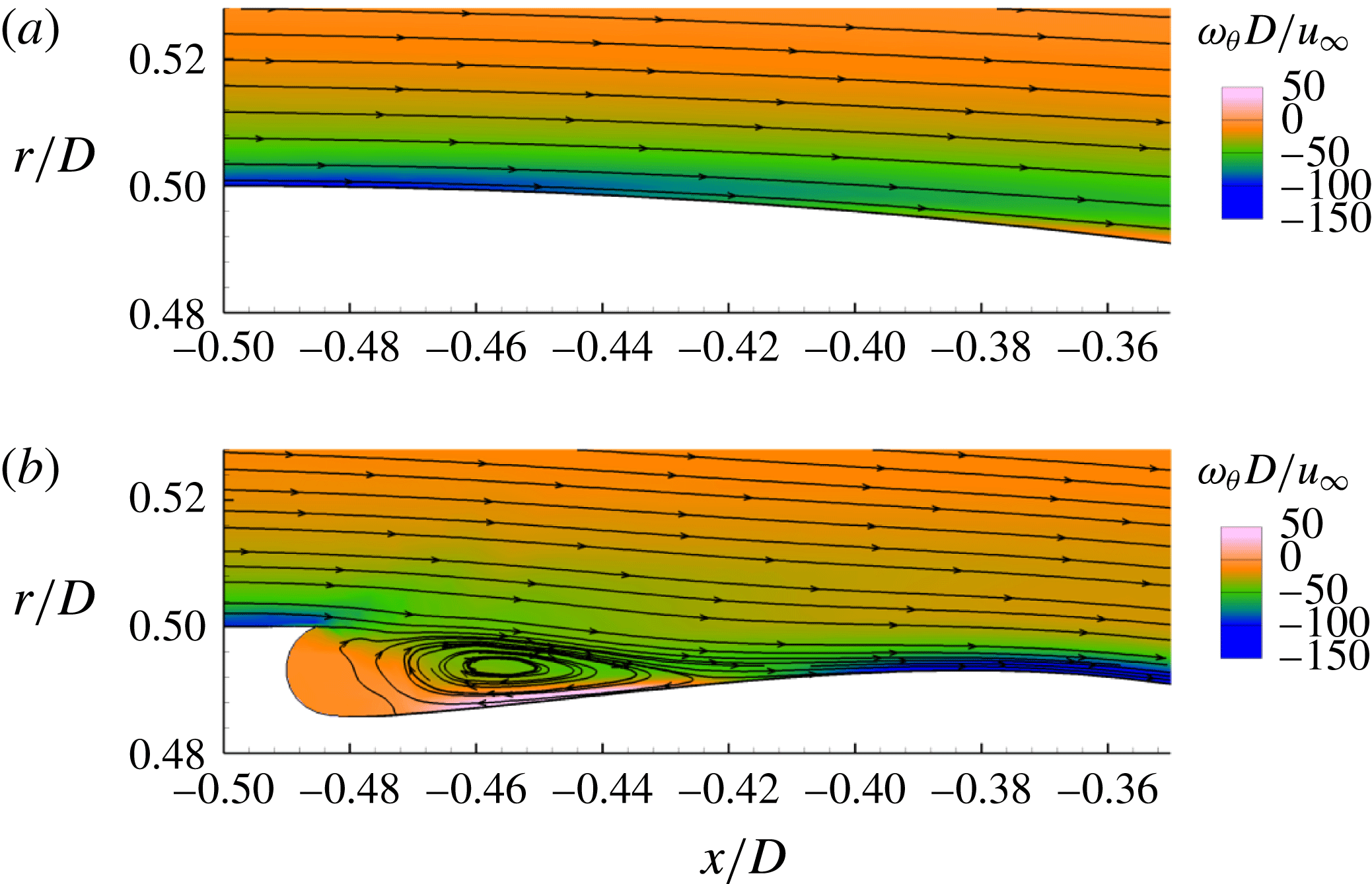
are immediately connected with the vorticity field. The magnitude of the azimuthal component of the vorticity is then shown, together with some streamlines, in figures 15(a) and 15(b), respectively for the boat tail without and with groove, for a flow region around the groove of the
 $d/D=0.791$
boat tail. The fields shown in figure 15(a,b) are instantaneous; however, they are representative for all the considered time instants since, as happens for the velocity and pressure, the vorticity fluctuations in the considered regions are very low. As can be seen, the magnitude of the vorticity within and outside the groove region is significantly smaller than that of the vorticity present near the surface of the plain boat tail. However, the thickness of the boundary layer just before and after the groove is smaller for the case of the grooved boat tail and this increases the near-wall vorticity in those regions. Furthermore, the fluid volume to be considered in the dissipation formula is obviously increased by the presence of the groove. Therefore, it is necessary to ascertain which is the effect of this variations on the enstrophy integral, not only around the groove but also more downstream, in the near wake.
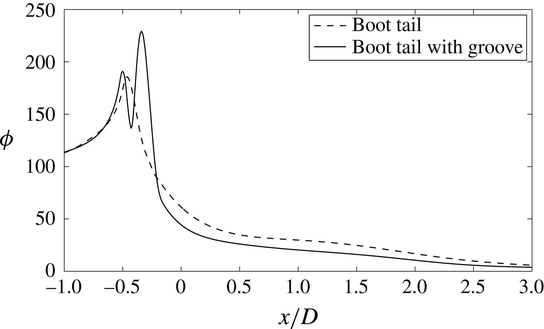
To this end, in figure 16 the axial variation is reported, for the same boat tail, of the following quantity:
 $$\begin{eqnarray}\unicode[STIX]{x1D6F7}(x)=\overline{\displaystyle \int _{S_{x}}\unicode[STIX]{x1D714}^{2}(x)\,\text{d}S_{x}},\end{eqnarray}$$
where
 $S_{x}$
is the surface comprising the whole fluid domain at a constant axial coordinate and the overline denotes the time average of the instantaneous values of the integral obtained during the whole simulations. The figure extends from the surface with axial coordinate
 $x/D=-1.0$
to a cross-section in the wake at
 $x/D=3.0.$
This choice is justified by the fact that the value of the enstrophy integral upstream and downstream of these planes is practically unchanged by the introduction of the grooves. Figure 15 immediately permits us to understand which are the regions where the dissipation varies due to the introduction of the groove. In particular, the curves in figure 16 confirm the prediction that, compared to the case without groove,
 $\unicode[STIX]{x1D6F7}(x)$
is smaller in the region of the groove, in spite of the larger volume, and larger immediately upstream and, specially, downstream of the groove. Nonetheless, it may be seen that the effect of the groove is to produce, more downstream, a significant reduction of
 $\unicode[STIX]{x1D6F7}(x)$
and, consequently, an appreciable reduction of the integral of the enstrophy in the whole considered domain. Indeed, the ratio between the integrals of
 $\unicode[STIX]{x1D6F7}(x)$
for the boat tails with and without grooves in the axial range of figure 16 is found to be equal to 0.921.
Integral of enstrophy along the computational domain at different
 $x/D$
sections.

3.4 Wake dynamics
Experimental standard deviation of the
 $x$
-velocity fields downstream of the
 $d/D=0.632$
boat tail. Plain boat tail: (a)
 $y/D=0$
, (b)
 $x/D=1.5$
. Boat tail with groove: (c)
 $y/D=0$
, (d)
 $x/D=1.5$
. The mean flow streamlines are also shown in (b,d).

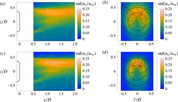
Finally, we briefly investigate on the effects of boat tailing and of the groove on the near-wake dynamics. At the Reynolds numbers of the present investigation, the wake flow of an axisymmetric body is characterized by the periodic shedding of hairpin-shaped vortices, each one composed of two streamwise legs and one final cross-flow portion. These vortices originate from the shear layers bounding the near-wake recirculation region and produce an instantaneously non-axisymmetric flow configuration having a symmetry plane. The orientation of this plane tends to change from cycle to cycle, either with a low angular velocity rotation or more randomly, thus producing an average symmetric wake. However, one particular plane may be fixed by proper perturbations introduced in the wake (Grandemange et al. Reference Grandemange, Gohlke, Parezanovic and Cadot2012; Vilaplana et al. Reference Vilaplana, Grandemange, Gohlke and Cadot2013; Grandemange, Gohlke & Cadot Reference Grandemange, Gohlke and Cadot2014; Rigas et al. Reference Rigas, Oxlade, Morgans and Morrison2014; Gentile et al. Reference Gentile, van Oudheusden, Schrijer and Scarano2017).
The configuration of the present wind tunnel tests, which is the same used in Mariotti & Buresti Reference Mariotti and Buresti2013, is such that the model support causes the stabilization of a vortex shedding with a vertical plane of symmetry. This can be appreciated from figure 17 showing the time-mean standard deviations of the axial velocity fluctuations in a longitudinal and in a cross-flow cross section for the
 $d/D=0.632$
case. Indeed, the vertical longitudinal cross-section immediately shows that the wake is non-axisymmetric in that plane due to the presence of the support, as already found in Mariotti & Buresti (Reference Mariotti and Buresti2013) for the blunt-based reference body. Furthermore, in the transverse wake cross-section the regions with higher fluctuations are restricted to a sector in the upper region, where the passage of the hairpin vortices occurs, as demonstrated by the cross-flow streamlines that are reported in the figures. This confirms that the symmetry plane of the shed vortices is predominantly vertical. The introduction of the grooves does not qualitatively change these mechanisms, although the distance between the legs of the hairpin vortices are reduced and their vertical location is moved slightly toward the axis. This is consistent with the previous observation that the introduction of the groove reduces the mean width of the near wake.
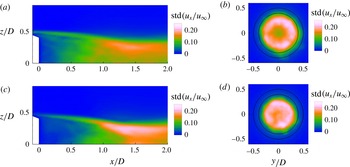
Figure 18 shows the same quantities as in figure 17 for the
 $d/D=0.791$
numerical cases without and with groove. The main aspect to be highlighted is the practical axisymmetry of the cross-flow regions with higher intensity of the fluctuations, which may be presumed to correspond to those where the passage of the hairpin vortices occurs. This suggests that during the length of the simulation the symmetry plane of the hairpin vortices either rotates or changes randomly in such a way to cover the whole circumference of the wake, similarly to what happens for axisymmetric bodies in uniform flow (see, e.g. Grandemange et al.
Reference Grandemange, Gohlke and Cadot2014 and Rigas et al.
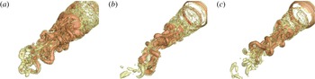
Reference Rigas, Oxlade, Morgans and Morrison2014). This is confirmed by the analysis of the instantaneous near-wake field as illustrated, by means of the instantaneous iso-surfaces of the vortex indicator
 $\unicode[STIX]{x1D706}_{2}$
(Jeong & Hussain Reference Jeong and Hussain1995), in figure 19, where the wake for the blunt-based body without boat tail is also shown. Both figures 18 and 19 show that, also in the numerical case, the wake dynamics, although significantly different from the experimental one, is not qualitatively altered by the introduction of boat tailing and of the groove, whose main effect is to reduce the wake width.
Numerical standard deviation of the
 $x$
-velocity fields downstream of the
 $d/D=0.791$
boat tail. Plain boat tail: (a)
 $y/D=0$
, (b)
 $x/D=1.5$
. Boat tail with groove: (c)
 $y/D=0$
, (d)
 $x/D=1.5$
.

Iso-surfaces of the vortex indicator
 $\unicode[STIX]{x1D706}_{2}$
(Jeong & Hussain Reference Jeong and Hussain1995) for (a) the body without boat tail (from Mariotti et al.
Reference Mariotti, Buresti and Salvetti2015a
), (b)
 $d/D=0.791$
boat tail, (c)
 $d/D=0.791$
boat tail with groove.

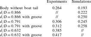
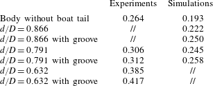
The shedding of the hairpin vortices induces velocity fluctuations in the near wake, with a dominating frequency that is a function of the wake width at the end of the recirculation region and, thus, of the boundary layer separation position. The Strouhal numbers obtained in the various experimental and numerical configurations, including the reference ones without boat tail, are reported in table 8. In all cases the effect of boat tailing and of the introduction of the grooves is evident and is consistent with the previously discussed behaviour of the wake widths. However, a difference may be noted between the values of the Strouhal numbers of the experimental and numerical data, with the latter that are appreciably lower for analogous geometry and flow conditions. Assuming that the shedding frequency is directly and inversely proportional respectively to a reference wake velocity and width, this finding suggests that the numerical wakes tend to be wider and/or with a lower characteristic velocity. The origin of this difference may possibly be due to the different turbulence levels of the free stream and of the separating boundary layers and to the non-axisymmetry of the experimental wakes due to the interference of the model support. Clearly, significant further work is needed to fully characterize and understand the wake dynamics for both experiments and simulations. However, based on the previous results, the action of the grooves does not seem to be related with substantial changes in the wake dynamics, at variance with what recently observed in García de la Cruz, Oxlade & Morrison (Reference García de la Cruz, Oxlade and Morrison2017) for a different passive control technique applied to a blunt-based bluff body.
Strouhal number evaluated from the velocity signals measured outside the wake edges at
 $x/D=1.5$
.
4 Preliminary robustness analysis
In order to gain an idea of the sensitivity of the separation-delay performance of contoured transverse grooves to the variation of the parameters defining their geometry, a few additional VMS-LES simulations were carried out for the boat tail with
 $d/D=0.791$
. In particular, the effects of the variation of the distance from the start of the boat tail,
 $s$
, and of the depth of the groove,
 $h$
, were analysed by carrying out simulations with two more values of each parameter, the other one being kept fixed at the value reported in table 2.
Considering first the position of the groove, the reference value
 $s/D=0.015$
corresponded to a groove placed practically at the start of the boat tail. Therefore, the two supplementary values,
 $s/D=0.057$
and
 $s/D=0.155$
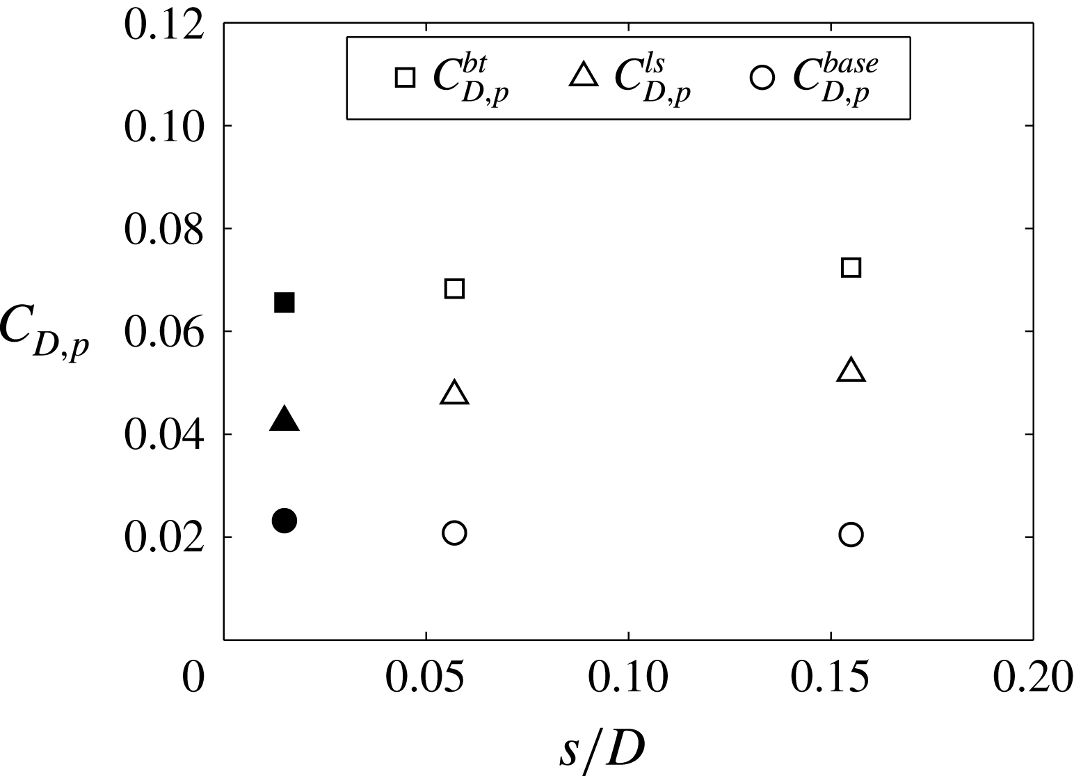
, were chosen in order to correspond to a downstream displacement of the groove. The results of the new simulations are compared with those of the reference case in figure 20, in terms of the total boat-tail pressure drag and of its single components, namely the contributions of the lateral surface and of the base. As can be seen, the total drag shows a limited increase with the downstream displacement of the groove. However, this variation derives from a small decrease of the base drag and a somewhat larger increase of the lateral surface drag.
Numerical pressure contributions to the boat-tail drag coefficient: effect of the variation of
 $s$
. Black symbols correspond to the reference groove.

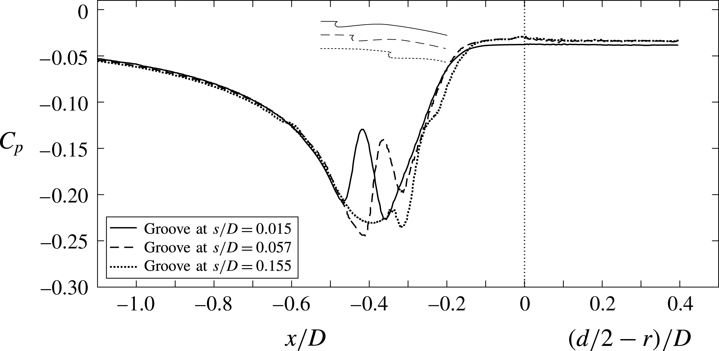
Numerical pressure coefficient over the lateral surface and the base, averaged in time and in the azimuthal direction. Sensitivity analysis to groove position
 $s/D$
.

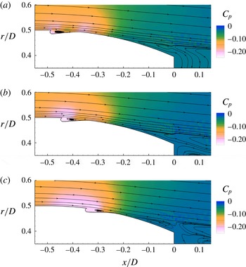
Mean flow streamlines and pressure field, both averaged in time and in the azimuthal direction. Groove at (a)
 $s/D=0.015$
(reference groove), (b)
 $s/D=0.057$
, (c)
 $s/D=0.155$
.

These results may be better interpreted by analysing figure 21, which shows the pressure distributions along the lateral and base surfaces of the different configurations. It is seen that the two grooves placed more downstream produce a slightly higher base pressure, corresponding to a delay of the separation compared to the reference groove; however, this does not compensate the negative effect of the increased suctions caused on the lateral side. In fact, if the objective is the reduction of the total drag, the figure suggests that the best results may be obtained when the groove position coincides with the region of minimum pressure for the plain boat tail (see also figure 5). A more global view of the flow conditions is given by figure 22, where the streamlines are superposed on the pressure field. In particular, it is clear that the downstream displacement of the groove causes an extension of the more negative
 $C_{p}$
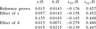
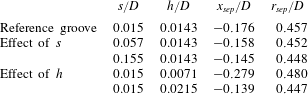
values towards regions where the surface normal vector has a larger axial component. Furthermore, it is seen that the streamlines bounding the reattachment region after the groove-induced recirculation have a lower concave curvature and this promotes a weaker local increase in pressure, as can indeed be observed in figure 21. Finally, the positions of the separation points corresponding to all the supplementary geometries analysed in the present section are compared to those of the reference case in table 9. By recalling that for the plain boat tail with the same diameter ratio the coordinates of the boundary layer separation point have been found to be
 $x_{sep}/D=-0.327$
and
 $r_{sep}/D=0.488$
, it can be seen that in all cases the groove produces a significant delay of the boundary layer separation and that the location of the groove has only a limited impact on this effect.
As for the influence of the depth of the groove, the reference one was
 $h/D=0.0143$
and it was then decided to analyse the effect of a
 $50\,\%$
decrease and increase of this value; therefore, the supplementary depths corresponded to
 $h/D=0.0071$
and
 $h/D=0.0215$
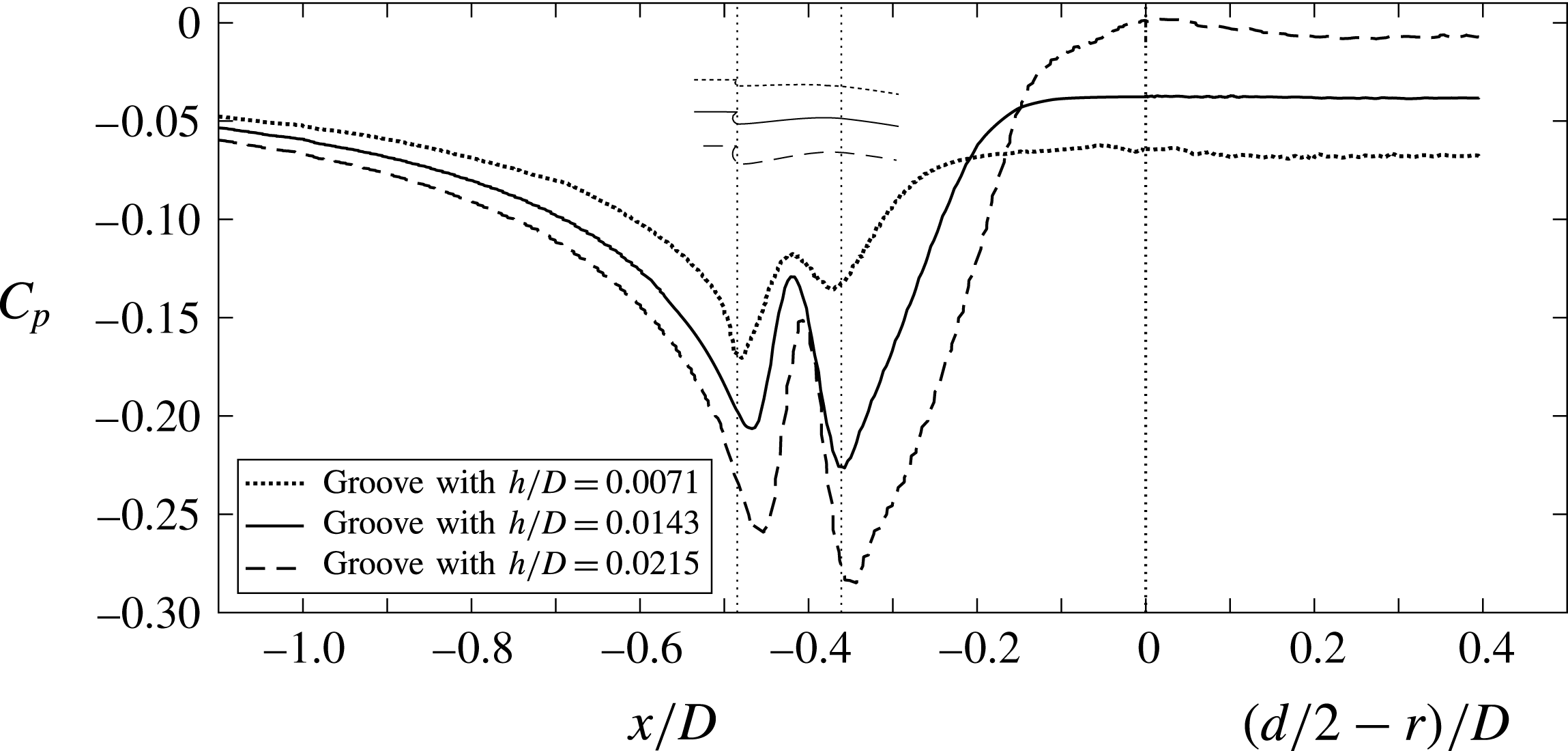
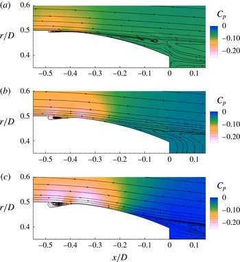
. The variations induced by these new geometries on the total, lateral and base pressure drags may be appreciated from figure 23, while figures 24 and 25 show, respectively, the surface pressure distributions and the streamlines superposed on the pressure field.
Numerical separation points for the supplementary grooves,
 $d/D=0.791$
.
Numerical pressure contributions to the boat-tail drag coefficient: effect of the variation of
 $h$
. Black symbols correspond to the reference groove.

Numerical pressure coefficient over the lateral surface and the base, averaged in time and in the azimuthal direction. Sensitivity analysis to groove depth
 $h/D$
.

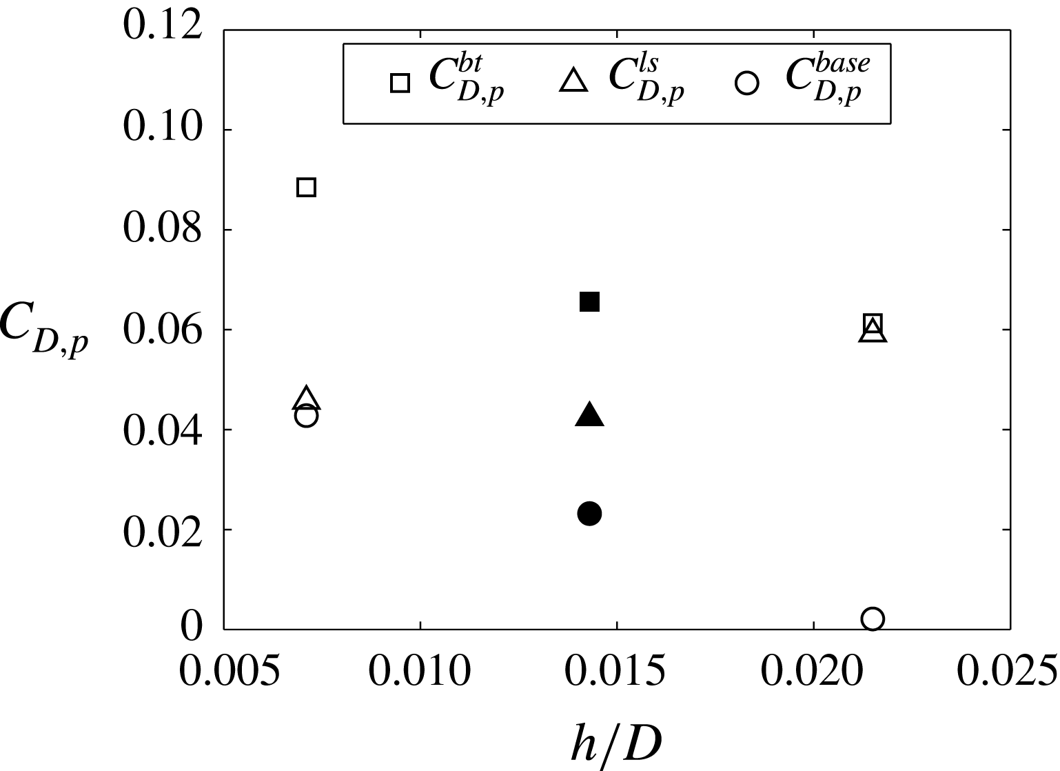
The differences between the various cases are now seen to be more significant. The most evident result is that the delay in boundary layer separation considerably increases with the depth of the groove (see also table 9). Thus, the increase of the depth causes a progressively stronger pressure recovery on the base and, consequently, a continuous decrease of the base drag, which even becomes negligible for the groove with
 $h/D=0.0215$
. However, for this deepest groove the lateral surface drag significantly increases compared to the reference case and this almost counterbalances the decrease of base drag. On the other hand, for the smallest groove with
 $h/D=0.0071$
only a small increase is found in the lateral pressure drag but, due to the lower base pressure, the total drag increases by approximately
 $35\,\%$
compared to the reference case, reaching a value that is not much lower than the one of the plain boat tail (see table 3). In effect, as is apparent from figure 25(a), this groove produces a very small recirculation, which influences only marginally the curvature of the streamlines and, hence, produces only a small delay of flow separation.
The effect of the depth of the groove on its separation-delay performance may also be directly connected with the value of the velocity along the streamline bounding the small recirculation region embedded in the groove. The velocity magnitude is obviously zero at the extremities of this streamline and reaches a maximum above the central region of the recirculation. The value of this bounding-streamline velocity increases with
 $h/D$
; more precisely, for the three increasing groove depths the maximum velocity values were found to be
 $u/u_{\infty }=0.097,$
 $0.180,$
 $0.256$
, and the average values
 $u/u_{\infty }=0.063,$
 $0.126,$
 $0.191$
. As previously discussed in § 3.3, this effect on the outer flow justifies the increasing separation-delay performance of the depth of the groove.
Mean flow streamlines and pressure field, both averaged in time and in the azimuthal direction. Groove having (a)
 $h/D=0.0071$
, (b)
 $h/D=0.0143$
(reference groove) (c)
 $h/D=0.0215$
.

Numerical boundary layer characteristics averaged in the azimuthal direction for
 $d/D=0.791$
: effect of the variation of
 $h$
. Mean
 $x$
-velocity at (a)
 $x/D=-0.50$
, (b)
 $x/D=-0.46$
, (c)
 $x/D=-0.35$
; standard deviation of the
 $x$
-velocity at (d)
 $x/D=-0.50$
, (e)
 $x/D=-0.46$
, (f)
 $x/D=-0.35$
.

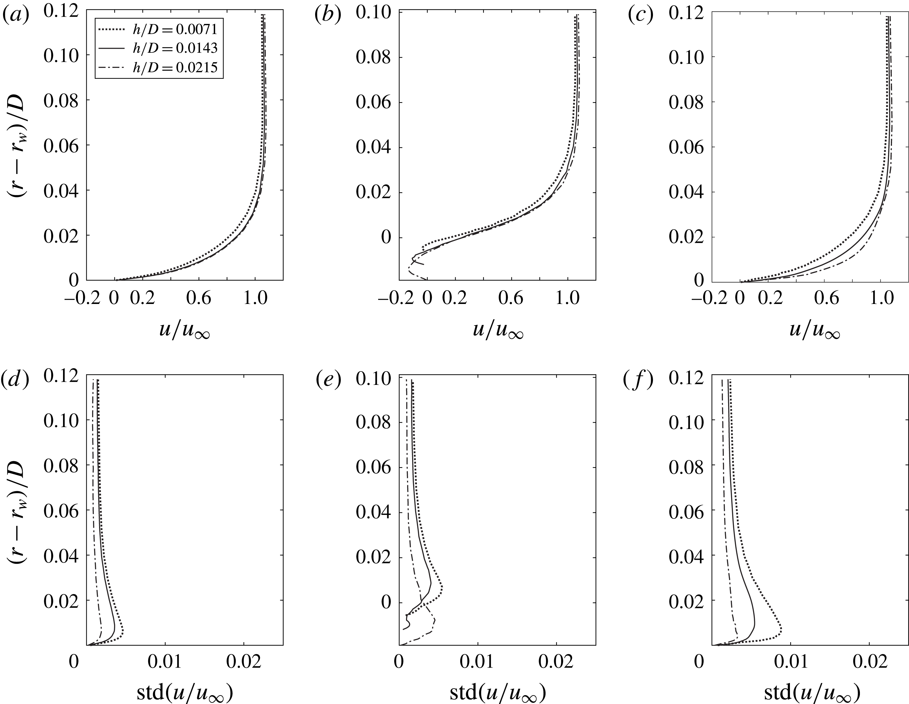
From the discussion of the results shown in figure 12 of the previous section, the groove with
 $s/D=0.015$
and
 $h/D=0.0143$
has already been presumed to assure a steady recirculating flow and no increase of the downstream fluctuations. Now, the improved performance of the deeper groove with
 $h/D=0.0215$
suggests the opportunity to check whether the same flow behaviour could be expected also in this case. To this end, the profiles of the mean value and of the standard deviation of the axial velocity are shown in figure 26 for the same positions considered in figure 12. In this case the comparison refers to the three different depths of the groove. It is apparent that the deepest groove, besides the expected higher near-wall momentum – which justifies its higher performance in delaying separation – shows a lower fluctuation level both upstream and downstream of the groove.
This result permits us to confidently infer that also in this case the flow field in the region around the groove is steady. Actually, this idea is also strongly substantiated by the fact that the separation lines around the body were always found to be remarkably steady in time, without any significant oscillation in the axial or in the azimuthal directions. Nonetheless, a note of caution might derive from figure 26(e), where it is seen that for the deepest groove the maximum of the fluctuations occurs inside the recirculation within the groove, rather than outside it, as happens in the other cases, and this can be interpreted as a signal of incipient tendency to unsteadiness of the flow recirculating inside the deepest groove. Considering that, as can be derived from table 6, for this groove the ratio between the depth and the upstream boundary layer thickness is
 $h/\unicode[STIX]{x1D6FF}=0.43$
, this result confirms that, to assure the steadiness of the recirculating flow, the groove depth must be sufficiently smaller than the thickness of the incoming boundary layer.
5 Conclusions and future developments
In the present work the performance of contoured transverse grooves (CTGs) as a method to delay flow separation was investigated through VMS-LES simulations and wind tunnel tests. CTGs are small cavities with a suitable shape introduced in a surface transversely to the incoming flow. The method was applied to an axisymmetric body characterized by a length to diameter ratio
 $L/D=5.714$
and by boat tails with various diameter ratios
 $d/D$
, so that reference conditions with different degrees of boundary layer separation could be analysed.
The shape of the grooves was carefully chosen to assure that the technique could reliably be considered as a really passive method. In other words, the aim was to obtain an intrinsically steady and stable flow, so that no active control be necessary for its successful operation. This led to the following choices in the groove design: the considered grooves start with a sharp edge and end with a spline leading to a point on the original boat-tail contour. The sharp edge is essential to fix the start of a local recirculation region embedded in the lower part of the boundary layer, and the gentle slope of the rear face avoids the presence of a rear sharp edge, which is the main perturbation source of rectangular grooves. Furthermore, as concerns the dimensions of the groove, its depth was constrained to be sufficiently smaller than the thickness of the incoming boundary layer (in the present work the maximum ratio
 $h/\unicode[STIX]{x1D6FF}$
was 0.43). All the above geometrical features are aimed at avoiding the self-sustained oscillations that are often found over small cavities and the instabilities that occur in vortices trapped inside transverse cavities that are much larger than the incoming boundary layers.
One single groove was introduced in the lateral surface of each of the considered boat tails, with geometrical parameters defined through a preliminary analysis using RANS simulations. A significant delay of the boundary layer separation was obtained for all the dimensions and positions of the grooves that were analysed experimentally and numerically in the present investigation. All the gathered evidence supports the conclusion that the physical mechanism responsible for the effectiveness of the contoured grooves as a separation-control method is the relaxation of the no-slip boundary condition for the flow surrounding the recirculation regions produced by the introduction of the grooves. Indeed, the obtained numerical and experimental results always confirmed that the flow inside the recirculation regions was steady and that no increase of the turbulence level occurred in the flow around and downstream of the grooves. Furthermore, the analysis of velocity spectra confirmed that no cavity resonance phenomena are present. On the other hand, the considerable mean velocity magnitudes found along the streamlines bounding the recirculations completely justify the increased near-wall momentum present in the downstream boundary layers and, consequently, their higher resistance to separation. Furthermore, a deeper analysis for a representative numerical case showed a significant decrease in enstrophy in the flow field around the groove and in the near wake, thus providing an assessment of the magnitude and spatial distribution of the reduction in viscous dissipation caused by the introduction of the grooves. Finally, all the numerical and experimental results confirm that the unsteady flow field phenomenology already found for an axisymmetric blunt-based body, with hairpin vortices being shed in the wake, is also present for boat-tailed bodies. However, as could be expected, the dimensions and shedding frequency of the vorticity structures are a function of the wake width which, in turn, depends on the position of the boundary layer separation. Therefore, the introduction of the grooves was found to produce an increase of the wake dominating frequency, with an order of magnitude that is quantitatively coherent with the separation-delay performance, without further significant modifications of the wake dynamics.
A few supplementary simulations were also carried out to investigate on the robustness of the effect of the grooves to variations of some of their geometrical parameters. In particular, starting from a CTG already giving a significant reduction of the separation extent and of the total drag of a boat tail, the effects produced by varying the position and the depth of the groove were analysed. As regards the groove position, it was found that the downstream displacement of the groove does not change significantly the total pressure drag as long as the groove is placed upstream of the separation occurring on the original boat tail. A higher effect is produced by the change of the depth of the groove. Indeed, the increase of the groove depth causes an increase of the maximum and average velocity along the streamline bounding the recirculation region embedded in the groove. Consequently, the separation is moved more downstream, thus causing a significant further decrease of the base drag, which, however, is almost counterbalanced by the simultaneous increase of the drag contribution of the lateral surface. In any case, the depth of the grooves must always satisfy the requirement of being sufficiently smaller than the incoming boundary layer thickness to avoid the possible onset of instabilities in the flow recirculating inside the cavity.
The limitation on the maximum depth of the grooves may also have an implication as regards the possible influence of a higher Reynolds number compared to the value of the present investigation. For a fixed geometry, i.e. for given shape of the body, increasing the Reynolds number implies a reduction of the non-dimensional boundary layer thickness and, consequently, of the maximum allowable ratio between groove depth and diameter. However, if the interest is on the dimensional value of the maximum depth, e.g. for technological reasons, then the situation changes if the increase in Reynolds number is due to an increase in reference velocity or in body dimension. Indeed, it is easy to see that an increase in velocity with unaltered dimension implies a reduction of the boundary layer thickness, and thus of the maximum allowable groove depth. Conversely, if the increase in Reynolds number is due to an increased dimension at constant velocity, the boundary layer would increase, together with the maximum allowable groove depth.
In summary, the success of the application of the grooves to the enhancement of the drag reducing performance of boat tails is a direct consequence of the effectiveness of this flow control technique in delaying flow separation. Future possible activities may concern both the optimization of the groove geometrical parameters for different applications and basic investigations aimed at obtaining a deeper understanding of the influence of those parameters on the physical mechanisms through which the flow field is modified by the grooves. In particular, one significant objective would be a clearer identification of the connection between the geometry of the grooves – and in particular their depth – and the appearance of flow instabilities. Furthermore, the possibility of obtaining a global reduction of the friction drag through the introduction of the grooves should be analysed. In this respect, a positive result depends on the possibility of obtaining a configuration for which the additional pressure drag of the groove cavity and the possible increase of the downstream friction do not counterbalance the reduction of friction drag over the surface extent corresponding to the recirculation produced by the groove. Probably, the success of this objective might imply the use of multiple consecutive grooves of small depth, whose performance in delaying separation would also be an interesting object of investigation. Finally, the analysis of the effectiveness of the grooves for two-dimensional configurations or for non-axisymmetric elongated bodies may be of interest both for applications and for fundamental fluid dynamics research.
Acknowledgements
The authors wish to thank the technical staff of the DICI Aerospace Engineering Division for the manufacturing of the wind tunnel models. Thanks are also due to G. Gennari for his contribution to the preliminary RANS analyses.